DESY 04-088

Edinburgh 2004/07

KIAS-P04026

The Neutralino Sector of the
Next-to-Minimal Supersymmetric Standard Model
S.Y. Choi¹, D.J. Miller² and P.M. Zerwas^3
1 Physics Department, Chonbuk National University, Chonju 561-756, Korea
² School of Physics, The University of Edinburgh, Edinburgh EH9 3JZ, Scotland
³ Deutsches Elektronen–Synchrotron DESY, D–22603 Hamburg, Germany

The Next–to–Minimal Supersymmetric Standard Model (NMSSM) includes a Higgs iso-singlet superfield in addition to the two Higgs doublet superfields of the minimal extension. If the Higgs fields remain weakly coupled up to the GUT scale, as naturally motivated by the concept of supersymmetry, the mixing between singlet and doublet fields is small and can be treated perturbatively. The mass spectrum and mixing matrix of the neutralino sector can be analyzed analytically and the structure of this 5–state system is under good theoretical control. We also determine decay modes and production channels in sfermion cascade decays to these particles at the LHC and pair production in $e^{+}e^{-}$ colliders.

1 Introduction

The Minimal Supersymmetric Standard Model (MSSM) [1, 2] opens the path to the analysis of supersymmetric theories. Arguments have been advanced however that suggest extensions beyond this minimal version. One well–motivated example is the Next–to–Minimal Supersymmetric Standard Model (NMSSM) [3] in which an iso–singlet Higgs superfield $\hat{S}$ is introduced in addition to the two iso–doublet Higgs fields $\hat{H}_{u,d}$ incorporated in the MSSM to generate electroweak symmetry breaking. Such an extension offers a possible solution of the $\mu$ problem, generating in a natural way, a value of the order of the electroweak breaking scale $v$; this is achieved by identifying $\mu$, apart from the ${\cal O}(1)$ coupling, with the vacuum expectation value of the scalar component $S$ of the new iso–singlet field. [For a recent summary of this construct see Ref.[4]; a useful code has been made available in Ref.[5].]

The superpotential of the NMSSM includes, besides the usual MSSM $W_{Y}$ Yukawa components, an additional term, which couples the iso–singlet to the two iso–doublet Higgs fields, plus the self–coupling of the iso–singlet:

$$W=W_{Y}+\lambda\hat{S}(\hat{H}_{u}\hat{H}_{d})+\frac{1}{3}\kappa\hat{S}^{3}$$ (1)

The two parameters $\lambda$ and $\kappa$ are dimensionless. By demanding the Higgs fields remain weakly interacting up to the GUT scale, the two couplings are bounded at the electroweak scale by the inequalities $\lambda,\kappa\raisebox{-3.69899pt}{~{}\shortstack{$<$\\ [-0.07cm] $\sim$}}~{}0.7$. While the scalar Higgs sector includes several soft supersymmetry breaking parameters, the Lagrangian of the gaugino/higgsino sector is complemented only by the familiar SU(2) and U(1) gaugino mass terms. As a result, the parameter space of the neutralino sector is much less complex than the Higgs space.

The superpotential without the singlet self–coupling, i.e. $\kappa=0$, incorporates a Peccei–Quinn (PQ) symmetry: $\{\hat{H}_{u}(1),\,\hat{H}_{d}(1),\,\hat{S}(-2),\,\hat{Q}(-1),\,\hat{U}(0),\,\hat{D}(0),\,\hat{L}(-1),\,\hat{E}(0)\}$. $\hat{Q}$ and $\hat{L}$ are the quark and lepton SU(2) doublet superfields, while $\hat{U}$, $\hat{D}$ and $\hat{E}$ are the up– and down–quark and lepton SU(2) singlet superfields respectively. The integer of each parenthesis indicates the PQ charge of the corresponding superfield. The spontaneous breaking of this symmetry by the non–zero vacuum expectation value $v_{s}/\sqrt{2}$ of the scalar $S$ field gives rise to a massless Goldstone boson. However, when $\kappa\neq 0$, the mass is lifted to a non–zero value by the self–interaction of the $S$ field. Still, a discrete $\mathbb{Z}_{3}$ symmetry is left which would lead to the formation of domain walls in the early Universe. This problem can be tamed by introducing new interactions of the inverse Planck size that, however, do not affect the low–energy effective NMSSM theory [6].

In contrast to the Higgs sector, masses and mixings in the chargino system are not affected by the singlet extension. [Of course new decays such as $S\rightarrow\tilde{\chi}^{+}\tilde{\chi}^{-}$ or $\tilde{\chi}^{+}\rightarrow\tilde{\chi}_{5}H^{+}$ may be possible if allowed kinematically.]

So far the supersymmetric particle spectrum of the NMSSM has received only little attention in the NMSSM literature, Refs.[3], [7]-[9]. In this report we attempt a systematic analytical analysis of the neutralino system. In contrast to the MSSM where exact solutions of the mass spectrum and mixing parameters can be constructed mathematically in closed form, this is not possible any more for the NMSSM in which the eigenvalue equation is of 5th order, not allowing closed solutions. However, since the coupling between singlet and doublet fields is weak, $\lambda v/\sqrt{2}\sim O(10^{2})\,{\rm GeV}$, compared with the typical supersymmetry scale $M_{1,2}$ and $\mu=\lambda v_{s}/\sqrt{2}\sim O(10^{3})\,{\rm GeV}$, a perturbative expansion of the solution gives rise to a good approximation of the mass spectrum while the magnitude of the matrix elements in the mixing matrix is at least qualitatively well understood. The usefulness of a perturbative expansion has also been noticed in Ref.[9]; however, here, extending the Higgs analysis in Ref.[4], we work out this approach systematically for all facets of the NMSSM.

While $\kappa$ plays a crucial rôle in the Higgs sector, it is less crucial for the neutralino system. The size of $\kappa v_{s}$, with $v_{s}\raisebox{-3.69899pt}{~{}\shortstack{$<$\\ [-0.07cm] $\sim$}}~{}15\,v$ to maintain a link with the electroweak scale, just determines the singlino mass before modified by mixing effects. Once masses and mixings are determined, the couplings of the neutralinos to the electroweak gauge bosons and to scalar/fermionic matter particles are fixed. Decay widths and production rates of the five neutralinos can subsequently be predicted for squark cascades at the LHC [10] and $e^{+}e^{-}$ annihilation at prospective linear colliders [11].

The report is organized as follows. In Sect. 2 we describe the neutralino sector of supersymmetric models in which the pair of Higgs doublet superfields is augmented by an additional iso-singlet field. In Sect. 3 we show how, for a naturally expected weak coupling, the properties of the four standard neutralinos are modified; moreover the properties of the fifth neutralino, the new singlino–dominated state, are calculated. All these spectra and mixings are pre–determined analytically before the surprisingly good quality of the weak–coupling expansion is demonstrated by comparison with numerical solutions. In this way we achieve a satisfactory theoretical understanding of the system. In the limit of large gaugino mass parameters $M_{1,2}$ compared with the higgsino mass parameter $\mu$, or vice versa, the MSSM part can be easily diagonalized analytically and a clear and simple picture of the entire system emerges. The section is concluded by a lovely toy model in which we set $M_{1}=M_{2}$ and $\tan\beta=1$; this set allows us to solve the system exactly, leading to transparent closed expressions for the neutralino mass spectrum and the mixing parameters. A sample of decay widths and production cross sections for the neutralinos is presented in Sect. 4. The results are summarized in Sect. 5 and technical details of the diagonalization procedure for the $5\times 5$ neutralino mass matrix are described in the Appendix.

2 The NMSSM Neutralino Sector

2.1 The NMSSM neutralino mass and mixing matrix

The Lagrangian of the neutralino system can be derived from the superpotential defined in Eq.(1), complemented by the SU(2) and U(1) mass terms in the soft supersymmetry breaking Lagrangian. After breaking the [electroweak] symmetry spontaneously by introducing non–zero vacuum expectation values of the iso-doublet and singlet Higgs fields,

$$\langle H_{u}\rangle=\frac{1}{\sqrt{2}}\sin\beta\,\left(\begin{array}[]{c}0\\ v\end{array}\right),\qquad\langle H_{d}\rangle=\frac{1}{\sqrt{2}}\cos\beta\,\left(\begin{array}[]{c}v\\ 0\end{array}\right),\qquad\langle S\rangle=v_{s}/\sqrt{2}$$ (6)

the Higgs–higgsino mass parameter

$$\mu=\lambda v_{s}/\sqrt{2}$$ (7)

is generated and, subsequently, the neutralino mass matrix

$${\cal M}_{5}=\left(\begin{array}[]{cc}{\cal M}&X\\ X^{T}&\mu_{\kappa}\end{array}\right)$$

with a hierarchical structure as analyzed in the Appendix, can be written in detail as:

$${\cal M}_{5}=\left(\begin{array}[]{cccc|c}M_{1}&0&-m_{Z}\,c_{\beta}\,s_{W}&m_{Z}\,s_{\beta}\,s_{W}&0\\ 0&M_{2}&m_{Z}\,c_{\beta}\,c_{W}&-m_{Z}\,s_{\beta}\,c_{W}&0\\ -m_{Z}\,c_{\beta}\,s_{W}&m_{Z}\,c_{\beta}\,c_{W}&0&-\mu&-\mu_{\lambda}\,s_{\beta}\\ m_{Z}\,s_{\beta}\,s_{W}&-m_{Z}\,s_{\beta}\,c_{W}&-\mu&0&-\mu_{\lambda}\,c_{\beta}\\[5.69054pt] \cline{1-4}\cr 0&0&-\mu_{\lambda}\,s_{\beta}&\lx@intercol\hfil-\mu_{\lambda}\,c_{\beta}\hfil\lx@intercol&\mu_{\kappa}\end{array}\right)$$ (14)

This $5\times 5$ mass matrix is constructed from the standard $4\times 4$ MSSM neutralino mass matrix ${\cal M}$ in the upper left corner, the mass term of the higgsino component $\tilde{S}$ of the singlet superfield $\hat{S}$,

$$\mu_{\kappa}=2\kappa\,v_{s}/\sqrt{2}$$ (15)

and the mixing between doublets and singlet parameterized by

$$\mu_{\lambda}=\lambda\,v/\sqrt{2}$$ (16)

The mass matrix ${\cal M}_{5}$ is defined in the group basis $(\tilde{B},\tilde{W}^{3},\tilde{H}^{0}_{d},\tilde{H}^{0}_{u},\tilde{S})$. As usual, $M_{1}$ and $M_{2}$ are the soft SUSY breaking U(1) and SU(2) gaugino mass parameters, $\tan\beta$ is the ratio of the vacuum expectation values of the two neutral SU(2) Higgs doublet fields (as defined in Eq. (6)), $s_{\beta}=\sin\beta$, $c_{\beta}=\cos\beta$, and $s_{W},c_{W}$, $t_{W}$ are the sine, cosine and tangent of the electroweak mixing angle $\theta_{W}$.

Since the neutralino mass matrix (14) is symmetric and real, it can be diagonalized by an orthogonal matrix $V^{5}$. The mass eigenvalues are real but not necessarily positive. They can be mapped onto positive values by supplementing the rotation matrix to $N^{5}=\Phi^{5}V^{5}$ with the diagonal phase matrix $(\Phi^{5})_{kl}=1(i)\,\delta_{kl}$ in case of positive (negative) eigenvalues so that $N^{5*}\,{\cal M}_{5}\,N^{5\dagger}$ is positive diagonal. The physical neutralino states $\tilde{\chi}^{0}_{i}$ $[i=1-4]$ are ordered according to ascending mass values while $\tilde{\chi}^{0}_{5}$ is the predominantly singlino state. They are mixtures

$$\tilde{\chi}^{0}_{i}=N^{5}_{ij}\,(\tilde{B},\tilde{W}^{3},\tilde{H}_{d},\tilde{H}_{u},\tilde{S})_{j}\qquad[i=1-5]$$ (17)

of the U(1), SU(2) gauginos, the doublet higgsinos and the singlino.

The unitary matrix $N^{5}$ defines the couplings of the mass eigenstates $\tilde{\chi}^{0}_{i}$ to other particles. For the neutralino production processes it is sufficient to consider the neutralino–neutralino–$Z$ vertices

$$\langle\tilde{\chi}^{0}_{iL}|Z|\tilde{\chi}^{0}_{jL}\rangle=-\frac{g}{2c_{W}}\left(N^{5}_{i3}N^{5*}_{j3}-N^{5}_{i4}N^{5*}_{j4}\right)$$

$$\langle\tilde{\chi}^{0}_{iR}|Z|\tilde{\chi}^{0}_{jR}\rangle=+\frac{g}{2c_{W}}\left(N^{5*}_{i3}N^{5}_{j3}-N^{5*}_{i4}N^{5}_{j4}\right)$$ (18)

and the fermion-sfermion-neutralino vertices

$$\langle\tilde{\chi}^{0}_{iR}|\tilde{f}_{L}|f_{L}\rangle=-\sqrt{2}\frac{g}{c_{W}}\left[I^{f}_{3}N^{5*}_{i2}c_{W}+(Q_{f}-I^{f}_{3})N^{5*}_{i1}s_{W}\right]$$

$$\langle\tilde{\chi}^{0}_{iL}|\tilde{f}_{R}|f_{R}\rangle=2g\,Q_{f}\,s_{W}N^{5}_{i1}$$ (19)

The coupling $g$ is the SU(2) gauge coupling, $I^{f}_{3}$ is the SU(2) isospin 3-component and $Q_{f}$ is the electric charge of the fermion $f$. In Eq. (19) the coupling to the higgsino component, which is proportional to the fermion mass, has been neglected for “light flavors”. The more involved Higgs couplings to the neutralinos are listed in detail in Sect. 4.

2.2 NMSSM parameter range

In contrast to the Higgs sector only two additional parameters $\lambda$ and $\kappa$ are introduced in the NMSSM neutralino sector as compared to that of the MSSM including $\mu$. Assuming that the fields remain weakly interacting up to the GUT scale, the two couplings are bounded at the electroweak scale by the inequality

$$\sqrt{\lambda^{2}+\kappa^{2}}\,\raisebox{-3.69899pt}{~{}\shortstack{$<$\\ [-0.07cm] $\sim$}}~{}\,0.7$$ (20)

Moreover, the renormalization group (RG) evolution of the couplings points to $\kappa\raisebox{-3.69899pt}{~{}\shortstack{$<$\\ [-0.07cm] $\sim$}}~{}\lambda$ as preferential target domain if the evolution starts from a random distribution of the couplings $\kappa_{U},\lambda_{U}\leq 2\pi$ at the GUT scale [4].

While $v=\sqrt{v^{2}_{u}+v^{2}_{d}}=246$ GeV is fixed by the Fermi coupling $G_{F}$, the parameter $v_{s}$ should be expected in the same range,

$$v_{s}\raisebox{-3.69899pt}{~{}\shortstack{$<$\\ [-0.07cm] $\sim$}}~{}15\,v$$ (21)

in compliance with the arguments for introducing the NMSSM. A RG analysis of the entire set of parameters shows that a low value of $\tan\beta$ is favored [4]. Current experimental analyses of $\tan\beta$ assume MSSM relations for the couplings; they are modified in the NMSSM and the results in this extended scenario are less restrictive.

Since the size of the doublet–singlet mixing is set by $\mu_{\lambda}=\lambda v/\sqrt{2}$, the mixing interaction is expected to be small compared with the standard supersymmetry scales, $\mu=\lambda v_{s}/\sqrt{2}$ and/or $M_{1,2}$ for which values $\raisebox{-3.69899pt}{~{}\shortstack{$<$\\ [-0.07cm] $\sim$}}~{}O(1\,{\rm TeV})$ are anticipated. As a result, transparent expressions can be found by performing a systematic expansion for small mixing between the gauginos/doublet higgsinos and the singlino, measured by the small size of the parameter $\mu_{\lambda}$ relative to the other parameters in the mass matrix.

In summary, at tree–level the NMSSM neutralino sector described above has six free parameters which we choose as $\mu_{\kappa}$ and $\mu_{\lambda}$ in addition to the MSSM parameters: $\left\{\{M_{1},M_{2},\tan\beta,\mu\};\mu_{\kappa},\mu_{\lambda}\right\}$. Sometimes it is convenient to re-express $\mu$, $\mu_{\lambda}$ and $\mu_{\kappa}$ in terms of $\lambda$, $\kappa$ and $v_{s}$. The spectrum of the NMSSM neutralino sector will now be analyzed in detail.

3 NMSSM Small–Mixing Scenarios

In general the diagonalization of the $5\times 5$ NMSSM mass matrix ${\cal M}_{5}$ cannot be performed analytically in closed form. However, if the doublet–singlet coupling is weak, an approximate analytical solution can be found after the $4\times 4$ MSSM submatrix ${\cal M}$ is analytically diagonalized following the elaborate standard procedures in Ref.[13].

The orthogonal matrix $V^{5}$ which transforms ${\cal M}_{5}$ to the diagonal mass matrix ${\cal M}^{D}_{5}={\rm diag}\,[m_{1},\ldots,m_{5}]$ is conveniently split into a matrix $V$ diagonalizing the $4\times 4$ submatrix ${\cal M}$ and a matrix performing subsequently the block diagonalization of the $4\times 4$ and $1\times 1$ submatrices. After the block–diagonalization, the upper left MSSM mass matrix ${\cal{M}}^{D}={\rm diag}\,[\tilde{m}_{1},\tilde{m}_{2},\tilde{m}_{3},\tilde{m}_{4}]$ needs not be re-diagonalized for small doublet–singlet mixing, as proved in the Appendix. The final result for the orthogonal matrix $V^{5}$ may be written in the simple form:

$$V^{5}\,\approx\,\left(\begin{array}[]{cc}11_{4\times 4}-\frac{1}{2}(V\Gamma)(V\Gamma)^{T}&(V\Gamma)\\[2.84526pt] -(V\Gamma)^{T}&1-\frac{1}{2}(V\Gamma)^{T}(V\Gamma)\end{array}\right)\,\left(\begin{array}[]{cc}V&0\\[2.84526pt] 0&11_{1\times 1}\end{array}\right)$$ (26)

The doublet–singlet 4–component mixing vector $\Gamma$ can be expressed in terms of the gaugino/higgsino parameters as

$$\Gamma=-\frac{\mu_{\lambda}}{{\rm det}({\cal M}-\mu_{\kappa})}\left(\begin{array}[]{c}M^{\prime}_{2}\,\mu\,m_{Z}\,s_{W}\,c_{2\beta}\\[2.84526pt] -M^{\prime}_{1}\,\mu\,m_{Z}\,c_{W}\,c_{2\beta}\\[2.84526pt] M^{\prime}_{1}\,M^{\prime}_{2}(\mu\,c_{\beta}-\mu_{\kappa}\,s_{\beta})-M^{\prime}_{12}\,m^{2}_{Z}\,s_{\beta}\\[2.84526pt] M^{\prime}_{1}\,M^{\prime}_{2}(\mu\,s_{\beta}-\mu_{\kappa}\,c_{\beta})-M^{\prime}_{12}\,m^{2}_{Z}\,c_{\beta}\end{array}\right)$$ (31)

with the abbreviations

$$M^{\prime}_{1}=M_{1}-\mu_{\kappa},\quad M^{\prime}_{2}=M_{2}-\mu_{\kappa},\quad M^{(\prime)}_{12}=M^{(\prime)}_{1}\,c^{2}_{W}+M^{(\prime)}_{2}\,s^{2}_{W}$$ (32)

and the determinant

$${\rm det}({\cal M}-\mu_{\kappa})=M^{\prime}_{1}M^{\prime}_{2}(\mu^{2}_{\kappa}-\mu^{2})+M^{\prime}_{12}(\mu\,s_{2\beta}+\mu_{\kappa})\,m^{2}_{Z}$$ (33)

The mixing with the singlet alters the MSSM mass eigenvalues $\tilde{m}_{i}$ $[i=1,\ldots 4]$ to $O(\varepsilon^{2})$, and correspondingly the singlet mass

$$\tilde{m}_{5}=\mu_{\kappa}$$ (34)

The shifts are given as

$$m_{i}=\tilde{m}_{i}+\frac{1}{\tilde{m}_{i}-\tilde{m}_{5}}\,(VX)^{2}_{i}\qquad[\,i=1-4]$$

$$m_{5}=\tilde{m}_{5}-\sum^{4}_{i}\frac{1}{\tilde{m}_{i}-\tilde{m}_{5}}\,(VX)^{2}_{i}$$ (35)

with the 4–component vector $X\equiv\mu_{\lambda}(0,0,-s_{\beta},-c_{\beta})$. [The eigenvalues are not necessarily ordered sequentially, and, if some of them are negative, the additional phase rotation transforms them to positive physical masses.] Even for small mixing, the 5th eigenvalue $m_{5}$ may differ significantly from the singlino mass parameter $\tilde{m}_{5}=\mu_{\kappa}$ if $\kappa$ is small. However, even though the relative shift may be large, the absolute shift remains small, of second order. Trivially, the eigenvalues fulfill the spur formula

$$\sum^{5}_{i=1}m_{i}=M_{1}+M_{2}+\mu_{\kappa}$$ (36)

which is independent of the parameters $\mu$ and $\mu_{\lambda}$.

The doublet–singlet mixing generates a singlino component in the wave functions of the original MSSM neutralinos $\tilde{\chi}^{0}_{i}$ $[\,i=1,\ldots,4\,]$ of the size

$$V^{5}_{i5}\,\approx\,\sum_{j=1}^{4}\,V_{ij}\Gamma_{j}$$ (37)

linear in the mixing parameter to first approximation as expected for off–diagonal elements. Reciprocally, the singlino component in the wave function of $\tilde{\chi}^{0}_{5}$ is reduced to

$$V^{5}_{55}\,\approx\,1-\frac{1}{2}\,\sum_{i=1}^{4}\Gamma^{2}_{i}$$ (38)

differing from unity only to second order in the mixing as expected for diagonal elements.

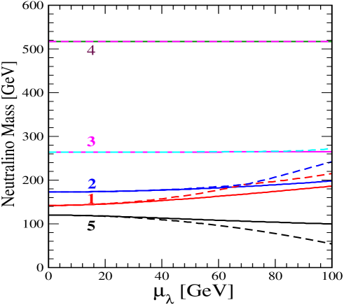
Figure 1: The exact numerical solution (solid) and the approximate solution (dashed) for the masses of the five neutralino states in the NMSSM as a function of $\mu_{\lambda}$ for the parameter set $\mathbb{P}=\{\mu_{\kappa}=120$ GeV, $M_{1}=250$ GeV, $M_{2}=500$ GeV, $\mu=170$ GeV, $\tan\beta=3\}$. The ordering of the mass spectrum is $m_{5},m_{1},m_{2},m_{3}$, and $m_{4}$ in increasing mass, i.e. the state $\tilde{\chi}^{0}_{5}$ is the lightest neutralino for the given parameter set.

As long as the mixing parameter $\mu_{\lambda}$ is significantly smaller than the other parameters, we find that the approximation works remarkably well, as demonstrated in Fig. 1. As an example both the exact numerical solutions and the approximate solutions for the neutralino masses are shown as a function of $\mu_{\lambda}$ for a favored parameter set $\mathbb{P}$ of broken PQ symmetry, $\mu_{\kappa}=120$ GeV with $M_{1}=250$ GeV, $M_{2}=500$ GeV, $\mu=170$ GeV and $\tan\beta=3$. The exact and approximate solutions agree rather well as long as $\mu_{\lambda}$ is less than about 80 GeV, as the mixing corrections are of second order in $\mu_{\lambda}$.

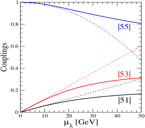
Figure 2: The exact numerical solution (solid) and the approximate solution (dashed) for the gaugino/higgsino and singlino components, $\{|N^{5}_{51}|,|N^{5}_{53}|,|N^{5}_{55}|\}$, of the lightest singlino–dominant neutralino as a function of $\mu_{\lambda}$ for the same parameter set $\mathbb{P}$ as in Fig.1.

In Fig. 2 the exact numerical solution (solid) and the approximate solution (dashed) are compared for the gaugino/higgsino and singlino components, $\{|(N^{5})_{51}|,|(N^{5})_{53}|,|(N^{5})_{55}|\}$, of the lightest singlino–dominated neutralino as a function of $\mu_{\lambda}$ for the same parameter set $\mathbb{P}$. Since the matrix $V^{5}$ is in general linear in the mixing term $\mu_{\lambda}$, the approximate solution differs from the exact solution already for smaller values of $\mu_{\lambda}$ in the reference point $\mathbb{P}$ in which $\tilde{m}_{5}=\mu_{\kappa}$ is quite close to the higgsino parameter $\mu$, though the characteristic features remain valid up to $\mu_{\lambda}\sim$ 40 GeV.

To fully exhaust the potential of our analytical method we perform the complete NMSSM diagonalization for the two standard limits analyzed in general within the MSSM: $M_{1,2}\gg|\mu|$ and vice versa, both complemented of course by small doublet–singlet mixing $\mu_{\lambda}\ll{\rm max}\{M_{1,2},|\mu|\}$.

3.1 Small singlino mass parameter

The first special analysis should be performed for small singlino mass parameter $\mu_{\kappa}$, which implies a slightly broken PQ symmetry $\kappa\ll 1$ as favored by the RG flow of this coupling in grand unified theories. Due to the small doublet–singlet mixing the structure of the original MSSM neutralinos $\tilde{\chi}^{0}_{i}$ $[i=1-4]$ is changed little while the properties of the 5th neutralino $\tilde{\chi}^{0}_{5}$, the lightest for small $\mu_{\kappa}$, are determined jointly by both the singlino parameter $\mu_{\kappa}$ and the mixing parameter $\mu_{\lambda}$.

3.1.1 Large gaugino mass parameters

As a first example, we consider the case with large gaugino mass parameters, i.e.  $M_{1,2}\gg|\mu|\gg m_{Z},\mu_{\lambda}$.

To begin, the $4\times 4$ diagonalization matrix $V$ defined in Eq. (26) can be parameterized up to second order according to standard MSSM procedure, cf. Ref.[13], as

$$V\approx\left(\begin{array}[]{cc}V_{G}&0\\[2.84526pt] 0&V_{H}\end{array}\right)\left(\begin{array}[]{cc}11_{2\times 2}&V_{X}\\[2.84526pt] -V^{T}_{X}&11_{2\times 2}\end{array}\right)\left(\begin{array}[]{cc}11_{2\times 2}&0\\[2.84526pt] 0&R_{\pi/4}\end{array}\right)$$ (45)

The $2\times 2$ $\pi/4$ rotation $R_{\pi/4}=(1-i\sigma_{y})/\sqrt{2}$ shifts the $[34]$ off–diagonal elements $[-\mu,-\mu]$ onto the diagonal axis $[\mu,-\mu]$. The second matrix, $V_{X}$,

$$V_{X}\,=\,\left(\begin{array}[]{cc}-c_{\beta}\,s_{W}\,m_{Z}/M_{1}&s_{\beta}\,s_{W}\,m_{Z}/M_{1}\\[8.53581pt] c_{\beta}\,c_{W}\,m_{Z}/M_{2}&-s_{\beta}\,c_{W}\,m_{Z}/M_{2}\end{array}\right)$$ (48)

removes the mixing between the blocks of the two gaugino and the two higgsino states. The components $V_{G}$ and $V_{H}$ diagonalize the gaugino and higgsino blocks themselves:

$$V_{G}\approx 11_{2\times 2}-\frac{1}{2}\left(\begin{array}[]{cc}s^{2}_{W}\,m^{2}_{Z}/M^{2}_{1}&0\\[5.69054pt] 0&c^{2}_{W}\,m^{2}_{Z}/M^{2}_{2}\end{array}\right)$$ (51)

$$V_{H}\approx 11_{2\times 2}-\frac{1}{2}\left(\begin{array}[]{cc}(1+s_{2\beta})\,M_{12}^{\prime\prime 2}m^{2}_{Z}/2M^{2}_{1}M^{2}_{2}&0\\[5.69054pt] 0&(1-s_{2\beta})\,M_{12}^{\prime\prime 2}m^{2}_{Z}/2M^{2}_{1}M^{2}_{2}\end{array}\right)$$ (54)

with $M_{12}^{\prime\prime 2}=M^{2}_{1}c^{2}_{W}+M^{2}_{2}s^{2}_{W}$, respectively. $V_{G}$ and $V_{H}$ relate to a diagonal form of the gaugino–higgsino mass matrix for large $M_{1,2}$ and $\mu$. Their off–diagonal matrix elements are of second order and can be omitted consistently as they would effect the eigenvalues only to fourth order.

After these steps are performed, the $4\times 4$ mass submatrix is diagonal and the complete symmetric mass matrix ${\cal M}_{5}$ takes the form

$${\cal M}_{5}\rightarrow\widehat{\cal M}_{5}\approx\left(\begin{array}[]{cccc|c}\tilde{m}_{1}&&&&0\\[2.84526pt] &{}\hskip 2.84526pt\tilde{m}_{2}&&&0\\[2.84526pt] &&\tilde{m}_{3}&&+\mu_{\lambda}c_{-}\\[11.38109pt] &&&\tilde{m}_{4}&-\mu_{\lambda}c_{+}\\[5.69054pt] \cline{1-4}\cr\\[-8.53581pt] 0&0&+\mu_{\lambda}c_{-}&\lx@intercol\hfil-\mu_{\lambda}c_{+}\hfil\lx@intercol&\mu_{\kappa}\end{array}\right)$$ (61)

where, in an obvious notation, zero elements are suppressed for easier reading, and $c_{\pm}=(c_{\beta}\pm s_{\beta})/\sqrt{2}$ is used as abbreviation. The MSSM neutralino mass eigenvalues are given by

$$\tilde{m}_{1}=M_{1}+\frac{m^{2}_{Z}}{M_{1}}s^{2}_{W}$$

$$\tilde{m}_{2}=M_{2}+\frac{m^{2}_{Z}}{M_{2}}c^{2}_{W}$$

$$\tilde{m}_{3}=\mu-\frac{M_{12}}{2M_{1}M_{2}}m^{2}_{Z}(1+s_{2\beta})$$

$$\tilde{m}_{4}=-\mu-\frac{M_{12}}{2M_{1}M_{2}}m^{2}_{Z}(1-s_{2\beta})$$ (62)

It remains to diagonalize $\widehat{\cal M}_{5}$ by choosing the proper form of $V\Gamma$ in $V^{5}$.

In the limit of large gaugino mass parameters, the doublet–singlet 4–component mixing vector $\Gamma$ reduces to a simple expression

$$\Gamma\approx\frac{\mu_{\lambda}}{\mu}\left(0,\,0,\,c_{\beta},\,s_{\beta}\right)^{T}$$ (63)

and the entire matrix $V^{5}$ can be written, up to second order, in the form

$$V^{5}\approx\left(\begin{array}[]{cccc|c}1&{}\hfil&{}\hfil&{}\hfil&0\\ {}\hfil&1&{}\hfil&{}\hfil&0\\[5.69054pt] {}\hfil&{}\hfil&1-\frac{\mu^{2}_{\lambda}}{4\mu^{2}}(1-s_{2\beta})&{}\hfil&\frac{\mu_{\lambda}}{\mu}\,c_{-}\\[5.69054pt] {}\hfil&{}\hfil&{}\hfil&1-\frac{\mu^{2}_{\lambda}}{4\mu^{2}}(1+s_{2\beta})&\frac{\mu_{\lambda}}{\mu}\,c_{+}\\[5.69054pt] \cline{1-4}\cr\\[-8.53581pt] 0&0&-\frac{\mu_{\lambda}}{\mu}\,c_{-}&\lx@intercol\hfil-\frac{\mu_{\lambda}}{\mu}\,c_{+}\hfil\lx@intercol&1-\frac{\mu^{2}_{\lambda}}{2\mu^{2}}\end{array}\right)\,\left(\begin{array}[]{cc}V&0\\[5.69054pt] 0&1\end{array}\right)$$ (72)

with zero’s suppressed in the upper $4\times 4$ matrix, and antisymmetric in the off–diagonal elements.

The rotations lead eventually to the diagonal mass matrix, of which the mass eigenvalues to the desired order are given by

$$m_{1}\approx M_{1}+\frac{m^{2}_{Z}}{M_{1}}s^{2}_{W}$$

$$m_{2}\approx M_{2}+\frac{m^{2}_{Z}}{M_{2}}c^{2}_{W}$$

$$m_{3}\approx\mu-\frac{M_{12}}{2M_{1}M_{2}}m^{2}_{Z}(1+s_{2\beta})+\frac{\mu^{2}_{\lambda}}{2\mu}(1-s_{2\beta})$$

$$m_{4}\approx-\mu-\frac{M_{12}}{2M_{1}M_{2}}m^{2}_{Z}(1-s_{2\beta})-\frac{\mu^{2}_{\lambda}}{2\mu}(1+s_{2\beta})$$

$$m_{5}\approx\mu_{\kappa}+\frac{\mu^{2}_{\lambda}}{\mu}s_{2\beta}$$ (73)

[recall $M_{12}=M_{1}c_{W}^{2}+M_{2}s_{W}^{2}$]. For the ordering of the eigenvalues and the flipping of the signs to positive physical masses the previous general remarks apply.

Two points should be emphasized explicitly. While the large gaugino masses $m_{1},m_{2}$ are not affected by the singlino, it does affect the higgsino states 3,4 to second order. The singlino mass is also affected to second order; however the mixing term can be leading if the singlino mass parameter $\mu_{\kappa}$ is small.

The mixing in the wave–functions is described by the components of $\Gamma$ itself [since the $4\times 4$ matrix $V$ deviates from unity only to second order in the small parameters of the order of the SUSY scales]:

$$V^{5}_{i5} \approx \frac{\mu_{\lambda}}{\mu}\left(0,\,0,\,-\frac{1}{\sqrt{2}}(c_{\beta}-s_{\beta}),\,-\frac{1}{\sqrt{2}}(c_{\beta}+s_{\beta})\right)_{\!i}$$

$$V^{5}_{5i} \approx \frac{\mu_{\lambda}}{\mu}\left(0,\,0,\,c_{\beta},\,s_{\beta}\right)_{\!i}$$

$$V^{5}_{55} \approx 1-\frac{\mu^{2}_{\lambda}}{2\mu^{2}}$$ (74)

3.1.2 Large higgsino mass parameter

As a second example, we consider the case with large higgsino mass parameter, i.e.  $|\mu|\gg M_{1,2}\gg m_{Z},\mu_{\lambda}$. This example is complementary to the previous case.

The overall diagonalization $4\times 4$ matrix $V$ can be parameterized in the same form as that in Eq.(45). The $2\times 2$ matrix $V_{X}$ describing the mixing between the two ensembles of the gaugino states and the higgsino states reads

$$V_{X}\approx\frac{m_{Z}}{\mu}\left(\begin{array}[]{cc}s_{W}\,s_{\beta}&-s_{W}\,c_{\beta}\\ -c_{W}\,s_{\beta}&c_{W}\,c_{\beta}\end{array}\right)$$ (77)

leading to a block-diagonal mass matrix composed of a $2\times 2$ matrix, depending on $M_{1}$ and $M_{2}$ with small corrections of the order of $m^{2}_{Z}/\mu$, and a $2\times 2$ mass matrix, depending only on the higgsino parameter $\mu$. The $2\times 2$ blocks $V_{G}$ and $V_{H}$ in the gaugino and higgsino sector may be written

$$V_{G}\approx 11_{2\times 2}-\frac{1}{2}\left(\begin{array}[]{cc}s^{2}_{W}\,m^{2}_{Z}/\mu^{2}&0\\[5.69054pt] 0&c^{2}_{W}\,m^{2}_{Z}/\mu^{2}\end{array}\right)$$ (80)

$$V_{H}\approx 11_{2\times 2}-\frac{1}{2}\left(\begin{array}[]{cc}\frac{1}{2}(1+s_{2\beta})\,m^{2}_{Z}/\mu^{2}&0\\[5.69054pt] 0&\frac{1}{2}(1-s_{2\beta})\,m^{2}_{Z}/\mu^{2}\end{array}\right)$$ (83)

respectively, after the higgsino submatrix has been diagonalized by the standard $R_{\pi/4}$ rotation.

These transformations diagonalize the $4\times 4$ submatrix within the block–diagonal matrix $\widehat{\cal M}_{5}$ of the same form as (61), of which the first four diagonal elements are given by

$$\tilde{m}_{1}=M_{1}-\frac{m^{2}_{Z}}{\mu}s^{2}_{W}\,s_{2\beta}$$

$$\tilde{m}_{2}=M_{2}-\frac{m^{2}_{Z}}{\mu}c^{2}_{W}\,s_{2\beta}$$

$$\tilde{m}_{3}=\mu+\frac{m^{2}_{Z}}{2\mu}(1+s_{2\beta})$$

$$\tilde{m}_{4}=-\mu-\frac{m^{2}_{Z}}{2\mu}(1-s_{2\beta})$$ (84)

The mixing between the doublet–higgsino and singlino states is then described in an analytic form by a 4–component column vector

$$\Gamma\approx\frac{\mu_{\lambda}}{\mu}\left(0,\,0,\,c_{\beta},\,s_{\beta}\right)^{T}$$ (85)

mixing the singlino both with the gauginos and with the doublet–higgsinos. The entire matrix $V^{5}$ can be written up to second order in the form, with antisymmetric off-diagonal elements,

$${}\hskip-14.22636ptV^{5}\!\approx\left(\begin{array}[]{cccc|c}1-\frac{\mu^{2}_{\lambda}m^{2}_{Z}s^{2}_{W}c^{2}_{2\beta}}{2M^{2}_{1}\mu^{2}}&{}\hfil&{}\hfil&{}\hfil&0\\[5.69054pt] {}\hfil&1-\frac{\mu^{2}_{\lambda}m^{2}_{Z}c^{2}_{W}c^{2}_{2\beta}}{2M^{2}_{2}\mu^{2}}&{}\hfil&{}\hfil&0\\[5.69054pt] {}\hfil&{}\hfil&1-\frac{\mu^{2}_{\lambda}c^{2}_{-}}{2\mu^{2}}&{}\hfil&\frac{\mu_{\lambda}c_{-}}{\mu}\\[5.69054pt] {}\hfil&{}\hfil&{}\hfil&1-\frac{\mu^{2}_{\lambda}c^{2}_{+}}{2\mu^{2}}&\frac{\mu_{\lambda}c_{+}}{\mu}\\[5.69054pt] \cline{1-4}\cr 0&0&-\frac{\mu_{\lambda}c_{-}}{\mu}&\lx@intercol\hfil-\frac{\mu_{\lambda}c_{+}}{\mu}\hfil\lx@intercol&1-\frac{\mu^{2}_{\lambda}}{2\mu^{2}}\end{array}\right)\left(\begin{array}[]{cc}V&0\\[5.69054pt] 0&1\end{array}\right)$$ (93)

and with the same abbreviations as before in Eq.(61).

The rotations lead eventually to a diagonal mass matrix, consisting of the mass eigenvalues:

$$m_{1}\approx M_{1}-\frac{m^{2}_{Z}}{\mu}s^{2}_{W}\,s_{2\beta}$$

$$m_{2}\approx M_{2}-\frac{m^{2}_{Z}}{\mu}c^{2}_{W}\,s_{2\beta}$$

$$m_{3}\approx\mu+\frac{m^{2}_{Z}}{2\mu}(1+s_{2\beta})+\frac{\mu^{2}_{\lambda}}{2\mu}(1-s_{2\beta})$$

$$m_{4}\approx-\mu-\frac{m^{2}_{Z}}{2\mu}(1-s_{2\beta})-\frac{\mu^{2}_{\lambda}}{2\mu}(1+s_{2\beta})$$

$$m_{5}\approx\mu_{\kappa}+\frac{\mu^{2}_{\lambda}}{\mu}s_{2\beta}$$ (94)

with apparent reciprocity in the MSSM subsystem between gaugino and higgsino parameters in comparison with the previous case, but universal modifications from the doublet–singlet mixing.

Correspondingly, to leading order the coefficients of $V^{5}$ involving the singlino index $5$ coincide with the elements of the doublet–singlet mixing matrix in Eq.(74).

3.2 Large singlino mass parameter

In the alternative extreme, the PQ symmetry is strongly broken if $\kappa$ is large and, equivalently, the singlino mass parameter is large, i.e. $\mu_{\kappa}\gg\mu_{\lambda},\mu,M_{1,2}$. This limit is not favored by the renormalization group flow from the GUT scale down to the electroweak scale but cannot be ruled out a priori on general grounds. The new fifth eigenstate, predominantly composed of the singlino, would in general be the heaviest state, mixed only weakly with the iso–doublets and, as a result, coupling weakly to electroweak gauge bosons and matter fields.

Applying the approximation method described in the Appendix and the general introduction to this section, the neutralino mass matrix can be transformed into the $4\times 4$ and $1\times 1$ block–diagonal form by inserting the mixing column vector

$$\Gamma\approx\frac{\mu_{\lambda}}{\mu_{\kappa}}\,\left(\,0,\,0,\,s_{\beta},\,c_{\beta}\,\right)^{T}$$ (95)

in the $V^{5}$ matrix Eq.(26). Note that the mixing column vector (95) is directly proportional to the 4–component off–diagonal column vector of the mass matrix (14) unlike the column vector (63) for a small singlino mass parameter.

From the general analysis it is apparent that the first four neutralino masses, of MSSM type, are modified to the order $\mu^{2}_{\lambda}/\mu_{\kappa}$ through the higgsino part, as is the 5th neutralino mass. The mass and the $55$ wave–function are approximately given by

$$m_{5}\approx\mu_{\kappa}+\frac{\mu^{2}_{\lambda}}{\mu_{\kappa}}$$ (96)

and

$$V^{5}_{55}\,\approx\,1-\frac{\mu^{2}_{\lambda}}{2\,\mu^{2}_{\kappa}}$$ (97)

while doublet components are mixed in to first order,

$$V^{5}_{5i}\approx-\frac{\mu_{\lambda}}{\mu_{\kappa}}\,\left(\,0,\,0,\,s_{\beta},\,c_{\beta}\,\right)$$ (98)

in parallel to the singlino components of the first doublet–type neutralinos.

In summary, the gaugino/doublet higgsino dominated neutralinos follow the pattern of the MSSM quite narrowly. Increasing the value of $\mu_{\kappa}$ will increase the mass of the new singlino state (almost) linearly, causing the state to decouple and making the NMSSM very difficult to distinguish from the MSSM.

3.3 The case with $M_{1}=M_{2}$ in the limit of $\tan\beta=1$

When the two soft–breaking SU(2) and U(1) gaugino masses are equal, $M_{1}=M_{2}=M$ and $\tan\beta=1$, cf. Ref.[13], the electroweak gauge symmetry guarantees the existence of a physical neutral state which does not mix with the other states and which has a mass eigenvalue identical to the modulus $M$. Furthermore, the gaugino states do not mix with the singlino state $\widetilde{S}$ that couples only to the specific linear combination of the higgsino states $\widetilde{H}^{0}_{b}=(\widetilde{H}^{0}_{u}+\widetilde{H}^{0}_{d})/\sqrt{2}$. As a result, one gaugino state mixes only with one higgsino state while the other orthogonal higgsino state mixes with the singlino state, leading to a block-diagonal matrix composed of one scalar and two $2\times 2$ matrices.

This special structure can be made apparent by switching to the mixed basis $\{\tilde{\gamma},\tilde{Z},\tilde{H}^{0}_{a},\tilde{H}^{0}_{b},\tilde{S}\}$ from the original group basis $\{\tilde{B},\tilde{W}^{3},\tilde{H}^{0}_{d},\tilde{H}^{0}_{u},\tilde{S}\}$ by means of the transformation

$$\left(\begin{array}[]{c}\tilde{\gamma}\\ \tilde{Z}\\ \tilde{H}_{a}\\ \tilde{H}_{b}\\ \tilde{S}\end{array}\right)={\cal A}_{5}\left(\begin{array}[]{l}\tilde{B}\\ \tilde{W}^{3}\\ \tilde{H}_{d}\\ \tilde{H}_{u}\\ \tilde{S}\end{array}\right)=\left(\begin{array}[]{rccrc}c_{W}&s_{W}&0&0&0\\ -s_{W}&c_{W}&0&0&0\\ 0&0&\frac{1}{\sqrt{2}}&-\frac{1}{\sqrt{2}}&0\\ 0&0&\frac{1}{\sqrt{2}}&\frac{1}{\sqrt{2}}&0\\ 0&0&0&0&1\end{array}\right)\left(\begin{array}[]{l}\tilde{B}\\ \tilde{W}^{3}\\ \tilde{H}_{d}\\ \tilde{H}_{u}\\ \tilde{S}\end{array}\right)$$ (119)

In this new $\{\tilde{\gamma},\tilde{Z},\tilde{H}^{0}_{a},\tilde{H}^{0}_{b},\tilde{S}\}$ basis the mass matrix $\widehat{\cal M}_{5}$ takes the block-diagonal form

$$\widehat{\cal M}_{5}={\cal A}_{5}{\cal M}_{5}{\cal A}_{5}^{T}=\left(\,\begin{array}[]{ccccc}\cline{1-1}\cr\vrule\lx@intercol\hfil M\hfil\lx@intercol\vrule\lx@intercol&0&0&0&0\\ \cline{1-3}\cr\lx@intercol\hfil 0\hfil\lx@intercol\vrule\lx@intercol&M&\lx@intercol\hfil m_{Z}\hfil\lx@intercol\vrule\lx@intercol&0&0\\ \lx@intercol\hfil 0\hfil\lx@intercol\vrule\lx@intercol&{}\,m_{Z}&\lx@intercol\hfil\mu\hfil\lx@intercol\vrule\lx@intercol&0&0\\ \cline{2-5}\cr 0&0&0&\vrule\lx@intercol\hfil-\mu\hfil\lx@intercol&\lx@intercol\hfil-\mu_{\lambda}\hfil\lx@intercol\vrule\lx@intercol\\ 0&0&0&\vrule\lx@intercol\hfil{}\,-\mu_{\lambda}\hfil\lx@intercol&\lx@intercol\hfil\mu_{\kappa}\hfil\lx@intercol\vrule\lx@intercol\\ \cline{4-5}\cr\end{array}\,\right)$$ (125)

This mass matrix generates two two–state mixings between $\tilde{Z}$ and $\tilde{H}^{0}_{a}$, and between $\tilde{H}^{0}_{b}$ and $\tilde{S}$, respectively. The block–diagonal matrix can be diagonalized by the orthogonal matrix

$$\hat{V}^{5}=\left(\begin{array}[]{ccc}1&{}\hfil&{}\hfil\\ {}\hfil&R_{g/h}&{}\hfil\\ {}\hfil&{}\hfil&R_{h/s}\end{array}\right)$$ (129)

consisting of two $2\times 2$ rotation matrices $R_{g/h}$ and $R_{h/s}$,

$$R_{g/h}=\left(\begin{array}[]{cr}\cos\theta_{g/h}&-\sin\theta_{g/h}\\ \sin\theta_{g/h}&\cos\theta_{g/h}\end{array}\right),\quad R_{h/s}=\left(\begin{array}[]{cr}\cos\theta_{h/s}&-\sin\theta_{h/s}\\ \sin\theta_{h/s}&\cos\theta_{h/s}\end{array}\right)$$ (134)

with the mixing angles determined by the relations

$$\tan\theta_{g/h}=-\frac{2\,m_{Z}}{M-\mu-\sqrt{(M-\mu)^{2}+4m^{2}_{Z}}}$$

$$\tan\theta_{h/s}=\frac{2\,\mu_{\lambda}}{\mu_{\kappa}+\mu+\sqrt{(\mu_{\kappa}+\mu)^{2}+4\mu^{2}_{\lambda}}}$$ (135)

The mass eigenvalues can be written completely in analytic form,

$$m_{1}=M$$

$$m_{2}=\frac{1}{2}\left(M+\mu+\sqrt{(M-\mu)^{2}+4m^{2}_{Z}}\right)$$

$$m_{3}=\frac{1}{2}\left(M+\mu-\sqrt{(M-\mu)^{2}+4m^{2}_{Z}}\right)$$

$$m_{4}=\frac{1}{2}\left(\mu_{\kappa}-\mu-\sqrt{(\mu_{\kappa}+\mu)^{2}+4\mu^{2}_{\lambda}}\right)$$

$$m_{5}=\frac{1}{2}\left(\mu_{\kappa}-\mu+\sqrt{(\mu_{\kappa}+\mu)^{2}+4\mu^{2}_{\lambda}}\right)$$ (136)

with the wave–functions of the neutralinos $\tilde{\chi}^{0}_{i}$ $[i=1,\ldots,5]$ determined by the cos/sin of the mixing angles $\theta_{g/h}$ and $\theta_{h/s}$.

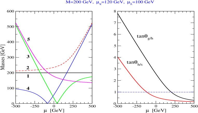
Figure 3: (a) The neutralino masses $|m_{i}|$, mapped onto positive values, and (b) the tangent values of the mixing angles $\theta_{g/h}$ and $\theta_{h/s}$ as a function of the higgsino mass parameter $\mu$ for the parameter set: $M=200$ GeV, $\mu_{\kappa}=120$ GeV, $\mu_{\lambda}=100$ GeV.

It is instructive to study the neutralino mass spectrum in this model for a set of fixed parameters $M=200$ GeV and $\mu_{\kappa}=120$ GeV, $\mu_{\lambda}=100$ GeV, by varying the higgsino mass parameter $\mu$. The branch character of the eigenvalues $\{23\}$ and $\{45\}$ is exemplified in Fig.3(a). The tan’s of the corresponding mixing angles are displayed in Fig.3(b). With rising tan’s we move from scenarios of no mixing, to maximal gaugino/doublet higgsino in $\{23\}$ and doublet/singlet higgsino mixing in $\{45\}$, finally to gaugino/doublet higgsino flipping $\{23\}$, and doublet/singlet flipping $\{45\}$, while the gaugino $\{1\}$ remains untouched.

4 Neutralino Production and Decays

In the MSSM the neutralino sector consists of two gauginos and two higgsinos. Typically the lightest supersymmetric particle (LSP), which is stable under the assumption of $R$-parity conservation, is the lightest state of the neutralino mass matrix. The LSP will appear as one of the final states of each sparticle decay and its non–observability is responsible for the well–known missing energy/momentum signature of supersymmetric particle production.

The neutralino production and decay properties in the NMSSM with the additional singlino state depend crucially on the singlino mass with respect to the MSSM neutralino masses [8]. If the singlino is much heavier than the other states, it will be very rarely produced and so practically unobservable. On the contrary, if the singlino is lighter than the other states, a singlino–dominated state will be the LSP so that the other neutralino states will decay, possibly through cascades, into the singlino–dominated LSP.

In this section, we present a qualitative description of the production of neutralinos, involving at least one singlino–dominated state, such as $\tilde{\chi}^{0}_{5}\tilde{\chi}^{0}_{5}$ and $\tilde{\chi}^{0}_{1}\tilde{\chi}^{0}_{5}$ and the subsequent decays of the neutralino $\tilde{\chi}^{0}_{1}$ into leptons and light Higgs bosons.

4.1 Singlino Production in $e^{+}e^{-}$ Annihilation

The production processes

$$e^{+}e^{-}\rightarrow\tilde{\chi}^{0}_{i}\tilde{\chi}^{0}_{j}\quad[i,j=1-5]$$ (137)

are generated by $s$–channel $Z$ exchange, and $t$– and $u$–channel $\tilde{e}_{L,R}$ exchanges. After appropriate Fierz transformations of the selectron exchange amplitudes [with the electron mass neglected], the transition matrix element of the production process can be written as

$$T(e^{+}e^{-}\rightarrow\tilde{\chi}^{0}_{i}\tilde{\chi}^{0}_{j})=\sum_{\alpha,\beta\,=L,R}Q_{\alpha\beta}\left[\bar{v}(e^{+})\gamma_{\mu}u(e^{-})\right]_{\alpha}\,\left[\bar{u}(\tilde{\chi}^{0}_{i})\gamma^{\mu}v(\tilde{\chi}^{0}_{j})\right]_{\beta}$$ (138)

The transition amplitudes are built up by the sum of the products of chiral neutralino currents and chiral fermion currents. The four generalized bilinear charges $Q_{\alpha\beta}$ correspond to independent helicity amplitudes, describing the neutralino production processes for polarized electrons/positrons [13]. They are defined by the fermion and neutralino currents and the propagators of the exchanged (s)particles as follows:

$$Q_{LL}=+\frac{D_{Z}}{s_{W}^{2}c_{W}^{2}}\,(I^{f}_{3}-Q_{f}s_{W}^{2}){\cal Z}_{ij}-D_{uL}g_{Lij},\quad Q_{RL}=-\frac{D_{Z}}{c_{W}^{2}}\,Q_{f}{\cal Z}_{ij}+D_{tR}g_{Rij}$$

$$Q_{LR}=-\frac{D_{Z}}{s_{W}^{2}c_{W}^{2}}\,(I^{f}_{3}-Q_{f}s^{2}_{W}){\cal Z}^{*}_{ij}+D_{tL}g^{*}_{Lij},\quad Q_{RR}=+\frac{D_{Z}}{c_{W}^{2}}Q_{f}{\cal Z}^{*}_{ij}-D_{uR}g^{*}_{Rij}$$ (139)

with $f=e^{-}$ in the production channel. The first term in each bilinear charge is generated by $Z$ exchange and the second term by selectron exchange; $D_{Z}$, $D_{tL,R}$ and $D_{uL,R}$ denote the $s$–channel $Z$ propagator and the $t$– and $u$–channel left/right–type selectron propagators

$$D_{Z}=\frac{s}{s-m^{2}_{Z}+im_{Z}\Gamma_{Z}},\qquad D_{(t,u)L,R}=\frac{s}{(t,u)-m^{2}_{\tilde{f}_{L,R}}}$$ (140)

with $s=(p_{e^{-}}+p_{e^{+}})^{2}$, $t=(p_{e^{-}}-p_{\tilde{\chi}^{0}_{i}})^{2}$ and $u=(p_{e^{-}}-p_{\tilde{\chi}^{0}_{j}})^{2}$ representing the Mandelstam variables for neutralino pair production in $e^{+}e^{-}$ collisions. Finally, the matrices ${\cal Z}_{ij}$, $g_{Lij}$ and $g_{Rij}$ are products of the neutralino diagonalization matrix elements $N^{5}_{ij}$

$${\cal Z}_{ij}=(N^{5}_{i3}N^{5*}_{j3}-N^{5}_{i4}N^{5*}_{j4})/2$$

$$g_{Lij}=\left(I^{f}_{3}N^{5}_{i2}c_{W}+(Q_{f}-I^{f}_{3})N^{5}_{i1}s_{W}\right)\left(I^{3}_{f}N^{5}_{j2}c_{W}+(Q_{f}-I^{f}_{3})N^{5}_{j1}s_{W}\right)^{*}/s_{W}^{2}c_{W}^{2}$$

$$g_{Rij}=Q^{2}_{f}N^{5}_{i1}N^{5*}_{j1}/c_{W}^{2}$$ (141)

The $e^{+}e^{-}$ annihilation cross sections follow from the squares of the bilinear charges,

$$\sigma\left[e^{+}e^{-}\rightarrow\tilde{\chi}^{0}_{i}\tilde{\chi}^{0}_{j}\right] = {\cal S}_{ij}\,\frac{\pi\alpha^{2}}{2s}\lambda_{\rm PS}^{1/2}\int^{1}_{-1}\bigg{\{}\left[1-(\mu^{2}_{i}-\mu^{2}_{j})^{2}+\lambda_{\rm PS}\cos^{2}\Theta\right]Q_{1}$$ (142)

$$\hskip 85.35826pt+4\mu_{i}\mu_{j}Q_{2}+2\lambda_{\rm PS}^{1/2}Q_{3}\cos\Theta\bigg{\}}\,d\cos\Theta\,$$

where ${\cal S}_{ij}$ is a statistical factor: 1 for $i\neq j$ and $1/2$ for $i=j$; $\mu_{i}=m_{\tilde{\chi}^{0}_{i}}/\sqrt{s}$, $\Theta$ is the polar angle of the produced neutrinos; and $\lambda_{\rm PS}=\lambda_{\rm PS}(1,\mu^{2}_{i},\mu^{2}_{j})$ denotes the familiar $2$–body phase space function $\lambda_{\rm PS}(x,y,z)\equiv x^{2}+y^{2}+z^{2}-2xy-2xz-2yz$. The quartic charges $Q_{i}$ ($i=1,2,3$) are given by the bilinear charges as follows:

$$Q_{1}=\frac{1}{4}\left[|Q_{RR}|^{2}+|Q_{LL}|^{2}+|Q_{RL}|^{2}+|Q_{LR}|^{2}\right]$$

$$Q_{2}=\frac{1}{2}\Re{\rm e}\left[Q_{RR}Q^{*}_{RL}+Q_{LL}Q^{*}_{LR}\right]$$

$$Q_{3}=\frac{1}{4}\left[|Q_{RR}|^{2}+|Q_{LL}|^{2}-|Q_{RL}|^{2}-|Q_{LR}|^{2}\right]$$ (143)

An example for the production of $\tilde{\chi}^{0}_{5}$ in association with another singlino–type ($\tilde{\chi}^{0}_{5}$), or a gaugino–type ($\tilde{\chi}^{0}_{1}$) or a higgsino–type ($\tilde{\chi}^{0}_{3}$) neutralino is presented in Fig.4 for the parameter set $\mathbb{P}$ [Fig.1] with $m_{\tilde{e}_{R}}=200$ GeV and $m_{\tilde{e}_{L}}=250$ GeV. [Of course the $\{55\}$ final state is unobservable without additional ISR $\gamma$ emission.] The increase of the cross sections with increasing doublet–singlet gaugino/higgsino mixing parameterized by $\mu_{\lambda}$ is obvious. The gaugino character of $\tilde{\chi}_{1}^{0}$ is responsible for the dominant size of the $\{51\}$ cross-section.

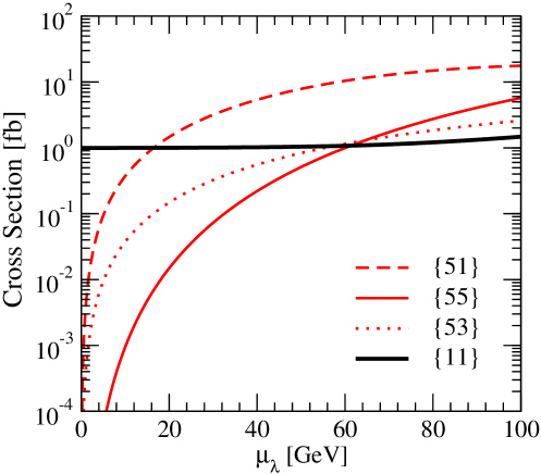
Figure 4: The production cross sections of neutralino pairs, $\{51\}$ (dashed), $\{55\}$ (thin–solid), $\{53\}$ (dotted) and $\{11\}$ (thick–solid), in $e^{+}e^{-}$ collisions with the center-of-mass energy $\sqrt{s}=500$ GeV as a function of $\mu_{\lambda}$ for the parameter set $\mathbb{P}$ [Fig.1] with $m_{\tilde{e}_{R}}=200$ GeV and $m_{\tilde{e}_{L}}=250$ GeV.

With the anticipated integrated luminosity $\int{\cal L}=1$ ab^-1, sufficiently large event rates of order 10³ are predicted if $\mu_{\lambda}$ is not too small.

4.2 Decays to a Singlino, with no Higgs bosons

(i) If kinematically allowed, two–body decays of neutralinos to the electroweak gauge bosons $Z$ are among the dominant channels. The widths of decays $\tilde{\chi}^{0}_{i}\rightarrow\tilde{\chi}^{0}_{j}Z$ are given by

$$\Gamma[\tilde{\chi}^{0}_{i}\!\rightarrow\!\tilde{\chi}^{0}_{j}Z]=\frac{g^{2}\lambda_{\rm PS}^{1/2}}{16\pi m_{\tilde{\chi}^{0}_{i}}}\left\{|{\cal Z}^{2}_{ij}|\!\!\left[\frac{(m^{2}_{\tilde{\chi}^{0}_{i}}\!-\!m^{2}_{\tilde{\chi}^{0}_{j}})^{2}}{m^{2}_{Z}}\!+\!m^{2}_{\tilde{\chi}^{0}_{i}}\!+\!m^{2}_{\tilde{\chi}^{0}_{j}}\!-\!2m^{2}_{Z}\right]\!+\!6m_{\tilde{\chi}^{0}_{i}}m_{\tilde{\chi}^{0}_{j}}\Re{\rm e}({\cal Z}^{2}_{ij})\!\right\}$$ (144)

where $\lambda_{\rm PS}=\lambda_{\rm PS}(1,m^{2}_{\tilde{\chi}^{0}_{j}}/m^{2}_{\tilde{\chi}^{0}_{i}},m^{2}_{Z}/m^{2}_{\tilde{\chi}^{0}_{i}})$, with ${\cal Z}_{ij}$ defined in Eq.(141). The widths of the chargino 2-body decays into a neutralino and a $W$ boson, $\tilde{\chi}^{\pm}_{i}\rightarrow\tilde{\chi}^{0}_{j}\,W^{\pm}$, read correspondingly

$$\hskip-22.76228pt\Gamma[\tilde{\chi}^{\pm}_{i}\rightarrow\tilde{\chi}^{0}_{j}\,W^{\pm}]=\frac{g^{2}\lambda_{\rm PS}^{1/2}}{16\pi m_{\tilde{\chi}^{\pm}_{i}}}\left\{\frac{|{\cal W}_{Lij}|^{2}+|{\cal W}_{Rij}|^{2}}{2}\left[\frac{(m^{2}_{\tilde{\chi}^{\pm}_{i}}-m^{2}_{\tilde{\chi}^{0}_{j}})}{m^{2}_{W}}+m^{2}_{\tilde{\chi}^{\pm}_{i}}+m^{2}_{\tilde{\chi}^{0}_{j}}-2m^{2}_{W}\right]\right.$$

$$\left.\hskip 142.26378pt-6\,m_{\tilde{\chi}^{\pm}_{i}}m_{\tilde{\chi}^{0}_{j}}\,\Re{\rm e}({\cal W}_{Lij}{\cal W}^{*}_{Rij})\right\}$$ (145)

where $\lambda_{\rm PS}=\lambda_{\rm PS}(1,m^{2}_{\tilde{\chi}^{0}_{j}}/m^{2}_{\tilde{\chi}^{\pm}_{i}},m^{2}_{W}/m^{2}_{\tilde{\chi}^{\pm}_{i}})$ and the bilinear charges ${\cal W}_{L,R}$ are defined as

$${\cal W}_{Lij}=U^{*}_{Li1}N^{5}_{j2}+\frac{1}{\sqrt{2}}U^{*}_{Li2}N^{5}_{j3},\quad{\cal W}_{Rij}=U^{*}_{Ri1}N^{5*}_{j2}-\frac{1}{\sqrt{2}}U^{*}_{Ri2}N^{5*}_{j4}$$ (146)

The unitary matrices $U_{L}$ and $U_{R}$ diagonalize the chargino mass matrix as $U_{R}{\cal M}_{C}U^{\dagger}_{L}={\rm diag}\left\{m_{\tilde{\chi}^{\pm}_{1}},m_{\tilde{\chi}^{\pm}_{2}}\right\}$, cf. Ref.[14] for details.

If 2–body decay channels are closed kinematically, the 3–body neutralino decays, $\tilde{\chi}^{0}_{i}\rightarrow\tilde{\chi}^{0}_{j}f\bar{f}$, are generated by $s$–channel (virtual) $Z$ exchange, and $t$– and $u$–channel sfermion exchanges. Neglecting fermion masses, the transition matrix element, cf. Ref.[15], is determined by the bilinear charges $Q^{\prime}_{\alpha\beta}$ which are related to the bilinear charges $Q_{\alpha\beta}$ introduced for the production, by crossing symmetry as

$$Q^{\prime}_{\alpha\beta}=Q^{*}_{\alpha\beta}$$ (147)

with the transformed Mandelstam variables, $s=(p_{f}+p_{\bar{f}})^{2}$, $t=(p_{\tilde{\chi}^{0}_{j}}+p_{\bar{f}})^{2}$ and $u=(p_{\tilde{\chi}^{0}_{j}}+p_{f})^{2}$ for the decays. [Neutralino decays to charginos and $W$ bosons can be described in the same way after obvious redefinitions of the bilinear charges.] Decay widths and distributions depend on the quartic charges $Q^{\prime}_{1}$, $Q^{\prime}_{2}$ and $Q^{\prime}_{3}$ defined analogously to Eq.(143).

(ii) At the LHC, cascade sfermion decays, $\tilde{f}\rightarrow f\tilde{\chi}^{0}_{i}$, are of great experimental interest. The width of the sfermion 2-body decay into a fermion and a neutralino follows from

$$\Gamma[\tilde{f}\rightarrow f\tilde{\chi}^{0}_{i}]=\frac{g^{2}\lambda_{\rm PS}^{1/2}}{16\pi m_{\tilde{f}}}\,|g_{\tilde{f}i}|^{2}\left(m^{2}_{\tilde{f}}-m^{2}_{\tilde{\chi}^{0}_{i}}-m^{2}_{f}\right)$$ (148)

where the 2–phase space function $\lambda_{\rm PS}=\lambda_{\rm PS}(1,m^{2}_{\tilde{\chi}^{0}_{i}}/m^{2}_{\tilde{f}},m^{2}_{f}/m^{2}_{\tilde{f}})$ with $\tilde{f}=\tilde{f}_{L}$ or $\tilde{f}_{R}$; the couplings are expressed in terms of the neutralino mixing matrix $N^{5}$ as

$$g_{\tilde{f}_{L}i}=\sqrt{2}\left[I^{f}_{3}N^{5}_{i2}+(Q_{f}-I^{f}_{3})N^{5}_{i1}t_{W}\right]\quad{\rm and}\quad g_{\tilde{f}_{R}i}=2Q_{f}s_{W}N^{5*}_{i1}$$ (149)

in obvious notation.

The reverse decays, neutralino [chargino] decays to sfermions plus fermions, $\tilde{\chi}^{0}_{i}\rightarrow\tilde{f}f$ etc, are given by the corresponding partial widths,

$$\Gamma[\tilde{\chi}^{0}_{i}\rightarrow\tilde{f}f]=\frac{g^{2}\lambda_{\rm PS}^{1/2}}{32\pi\,m_{\tilde{\chi}^{0}_{i}}}\,|g_{\tilde{f}i}|^{2}\left(m^{2}_{\tilde{\chi}^{0}_{i}}+m^{2}_{f}-m^{2}_{\tilde{f}}\right)$$ (150)

with the same couplings as before and $\lambda_{\rm PS}=\lambda_{\rm PS}(1,m^{2}_{\tilde{f}}/m^{2}_{\tilde{\chi}^{0}_{i}},m^{2}_{f}/m^{2}_{\tilde{\chi}^{0}_{i}})$. [Analogous expressions hold for chargino decays.]

Examples of these partial decay widths are shown in Fig.5 [with the parameter set $\mathbb{P}$ as in Fig.1]. For an illustrative purpose, the mass of the R–sleptons $\tilde{l}_{R}$ is assumed to be $m_{\tilde{l}_{R}}=200\,{\rm GeV}>m_{\tilde{\chi}_{1}^{0}}$ for the 3–body neutralino decays and to be $m_{\tilde{l}_{R}}=130\,{\rm GeV}<m_{\tilde{\chi}_{1}^{0}}$ for the 2–body slepton decays, respectively. The masses of the squarks are assumed to be $m_{\tilde{q}_{L}}=250$ GeV and $m_{\tilde{q}_{R}}=200$ GeV. For small mixing $\mu_{\lambda}$ the lifetimes of the second lightest neutralino $\tilde{\chi}^{0}_{1}$ and the R-sleptons $\tilde{l}_{R}$ can be quite large, giving rise potentially to macroscopic flight paths [9]. However, cosmological bounds on $\mu_{\lambda}$ must be analyzed before any (realistic) experimental conclusions can be drawn. The kink in the $\tilde{\chi}_{1}^{0}$ lifetime and flight distance in the upper right panel of Fig.5 is caused by accidental cancellations between sfermion and $Z$ exchange diagrams in the decays $\tilde{\chi}_{1}^{0}\to\tilde{\chi}_{5}^{0}\,q\bar{q}$ and $\tilde{\chi}_{5}^{0}\,\nu\bar{\nu}$; these accidental cancellations do not occur [to any significant degree] in the decay $\tilde{\chi}_{1}^{0}\to\tilde{\chi}_{5}^{0}\,l^{+}l^{-}$.

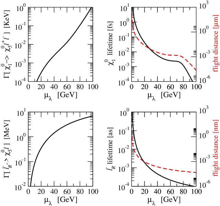
Figure 5: The widths, lifetimes and flight distances [broken lines] of the decays $\tilde{\chi}^{0}_{1}\rightarrow\tilde{\chi}^{0}_{5}\,l^{+}l^{-}$ and $\tilde{l}_{R}\rightarrow\tilde{\chi}^{0}_{5}l$ as a function of $\mu_{\lambda}$ for the parameter set $\mathbb{P}$[Fig.1]. The mass of the right–handed slepton is taken to be $m_{\tilde{l}_{R}}=200\,{\rm GeV}>m_{\tilde{\chi}_{1}^{0}}$ for the 3–body neutralino decays (upper panels) and to be $m_{\tilde{l}_{R}}=130\,{\rm GeV}<m_{\tilde{\chi}_{1}^{0}}$ for the 2–body slepton decays (lower panels). The masses of the squarks are assumed to be $m_{\tilde{q}_{L}}=250$ GeV and $m_{\tilde{q}_{R}}=200$ GeV. Right: flight distances for $\sqrt{s}=500$ GeV are shown by broken lines. The kink in the $\tilde{\chi}_{1}^{0}$ lifetime and flight distance in the upper right panel is caused by accidental cancellations between sfermion and $Z$ exchange diagrams. [The value of the lower bound, expected from cosmological arguments on $\mu_{\lambda}$ is presently not yet known.]

4.3 Decays to a Singlino, involving Higgs bosons

Decays involving Higgs bosons can be quite different for different Higgs boson mass spectra. Following the procedure outlined in Ref.[4] we decompose the neutral Higgs states into real and imaginary parts as follows:

$$H_{d}^{0} = \frac{1}{\sqrt{2}}\left[v_{d}-S_{1}s_{\beta}+S_{2}c_{\beta}+iP_{1}s_{\beta}\right],$$ (151)

$$H_{u}^{0} = \frac{1}{\sqrt{2}}\left[v_{u}+S_{1}c_{\beta}+S_{2}s_{\beta}+iP_{1}c_{\beta}\right],$$ (152)

$$S = \frac{1}{\sqrt{2}}\left[v_{s}+S_{3}+iP_{2}\right]$$ (153)

where the Goldstone states are removed by using the unitary gauge. We then further rotate these states onto the mass eigenstates, $H_{i}$ ($i=1-3$) and $A_{i}$ ($i=1,2$) labeled in order of ascending mass, by using the orthogonal rotation matrices $O^{H}$ and $O^{A}$:

$$H_{i}=S_{j}O^{H}_{ji},\qquad A_{i}=P_{j}O^{A}_{ji}$$ (154)

The resulting mass spectrum, composed of three scalars, two pseudocalars, and two charged Higgs bosons, is shown in Fig.6 as a function of $\mu_{\lambda}$. For the purposes of example, we have chosen the mass parameter $M_{A}$ (defined to be the heavy pseudoscalar mass in the MSSM limit) to be $2\mu/\sin 2\beta\approx 567$ GeV, setting the scale of the heavy Higgs bosons. The lighter Higgs bosons consist of two scalars and one pseudoscalar. The lightest scalar and pseudoscalar in our example are predominantly singlet states, with masses set by the scale of $\mu_{\kappa}$.

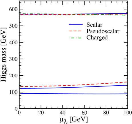
Figure 6: The Higgs boson mass spectrum as a function of $\mu_{\lambda}$ for the parameter set $\mathbb{P}$[Fig.1] and maximal mixing. For the purposes of example, the Higgs mass parameter $M_{A}$ is set to $2\mu/\sin 2\beta$. Heavy scalar, pseudoscalar and charged states are nearly mass degenerate: $M_{H_{3}}\simeq M_{A_{2}}\simeq M_{H^{\pm}}\simeq M_{A}$.

Generally, the width of a 2-body neutralino or chargino $\tilde{\chi}_{i}$ decay to a neutralino or chargino $\tilde{\chi}_{j}$ and a Higgs boson $\phi_{k}$ ($H_{k}$ or $A_{k}$) is given by

$$\Gamma[{\tilde{\chi}}_{i}\to{\tilde{\chi}}_{j}\phi_{k}] = \frac{\lambda_{\rm PS}^{1/2}}{16\pi m_{{\tilde{\chi}}_{i}}}\left\{\left(m_{{\tilde{\chi}}_{i}}^{2}+m_{{\tilde{\chi}}_{j}}^{2}-m_{\phi_{k}}^{2}\right)\left(|C^{L}_{ijk}|^{2}+|C^{R}_{ijk}|^{2}\right)\right.$$ (155)

$$\hskip 85.35826pt\left.+2\eta_{\phi}m_{{\tilde{\chi}}_{i}}m_{{\tilde{\chi}}_{j}}\left(C^{L}_{ijk}C^{R\,*}_{ijk}+C^{L\,*}_{ijk}C^{R}_{ijk}\right)\right\}$$

where $\lambda_{\rm PS}=\lambda_{\rm PS}(1,m_{{\tilde{\chi}}_{j}}^{2}/m_{{\tilde{\chi}}_{i}}^{2},m_{\phi_{k}}^{2}/m_{{\tilde{\chi}}_{i}}^{2})$ and the left/right couplings $C^{L/R}_{ijk}$ must be specified in each individual case; $\eta_{\phi}=1$ for $\phi=H_{k},\,H^{\pm}$, and $-1$ for $\phi=A_{k}$.

(i) For the decay of a neutralino $\tilde{\chi}^{0}_{i}$ to a neutralino $\tilde{\chi}^{0}_{j}$ and a scalar Higgs boson $H_{k}$, ${\tilde{\chi}^{0}}_{i}\to{\tilde{\chi}^{0}}_{j}H_{k}$, the couplings are given by,

$$C^{R}_{ijk}({\tilde{\chi}^{0}}_{i}\to{\tilde{\chi}^{0}}_{j}H_{k})\! = \!\frac{1}{2}\left[g(N^{5}_{i2}\!-\!N^{5}_{i1}t_{W})(\phantom{-}N^{5}_{j3}s_{\beta}\!+\!N^{5}_{j4}c_{\beta})\!+\!\sqrt{2}\lambda\left(N^{5}_{i3}c_{\beta}\!-\!N^{5}_{i4}s_{\beta}\right)N^{5}_{j5}\right]\!O^{H}_{1k}$$ (156)

$$+ \!\frac{1}{2}\left[g(N^{5}_{i2}\!-\!N^{5}_{i1}t_{W})(-N^{5}_{j3}c_{\beta}\!+\!N^{5}_{j4}s_{\beta})\!+\!\sqrt{2}\lambda\left(N^{5}_{i3}s_{\beta}\!+\!N^{5}_{i4}c_{\beta}\right)N^{5}_{j5}\right]\!O^{H}_{2k}$$

$$+ \frac{1}{\sqrt{2}}\left[\lambda N^{5}_{i3}N^{5}_{j4}-\kappa N^{5}_{i5}N^{5}_{j5}\right]\!O^{H}_{3k}\quad+\quad(i\leftrightarrow j)$$

$$C^{L}_{ijk}({\tilde{\chi}^{0}}_{i}\to{\tilde{\chi}^{0}}_{j}H_{k}) = C^{R\,*}_{ijk}({\tilde{\chi}^{0}}_{i}\to{\tilde{\chi}^{0}}_{j}H_{k})$$ (157)

While the first term in each of the two square brackets in Eq.(156) are reminiscent of the MSSM couplings $\tilde{\chi}_{i}^{0}{\tilde{\chi}}_{j}^{0}h$ and $\tilde{\chi}_{i}^{0}{\tilde{\chi}}_{j}^{0}H$ respectively, the other terms are genuinely new in origin, arising from the extra interaction terms in the NMSSM superpotential.

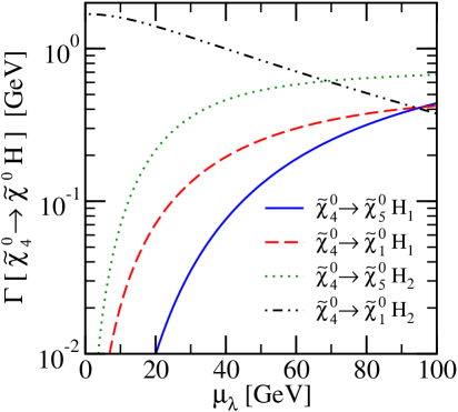
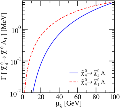
Figure 7: The decay widths for $\tilde{\chi}_{4}^{0}\to\tilde{\chi}_{1,\,5}^{0}H_{1,\,2}$ (left) and $\tilde{\chi}_{4}^{0}\to\tilde{\chi}_{1,\,5}^{0}A_{1}$ (right) for the parameter set $\mathbb{P}$[Fig.1] and maximal mixing. For the purposes of example, the Higgs mass parameter $M_{A}$ is set to $2\mu/\sin 2\beta$.

The widths for the kinematically allowed decays $\tilde{\chi}_{4}^{0}\to\tilde{\chi}_{1,5}^{0}H_{1,2}$ are shown in Fig.7 (left) as a function of $\mu_{\lambda}$. For $\mu_{\lambda}=0$ the $\tilde{\chi}_{5}^{0}$ state is decoupled from the other neutralinos; as $\mu_{\lambda}$ is switched on, the coupling, and therefore the decay widths, increase. The decay widths for $\tilde{\chi}_{4}^{0}\to\tilde{\chi}_{5}^{0}H_{1}$ and $\tilde{\chi}_{4}^{0}\to\tilde{\chi}_{5}^{0}H_{2}$ are comparable, within an order of magnitude, due to the large $\tilde{\chi}_{4}^{0}$ mass and the near mass degeneracy of $H_{1}$ and $H_{2}$. With partial widths of order GeV, these decay modes are in the observable range of branching ratios.

(ii) Similarly, a 2-body neutralino decay to a neutralino and a pseudoscalar Higgs boson, ${\tilde{\chi}}_{i}^{0}\to{\tilde{\chi}}_{j}^{0}A_{k}$, follows Eq.(155) with the left/right couplings given by

$$C^{R}_{ijk}({\tilde{\chi}^{0}}_{i}\to{\tilde{\chi}^{0}}_{j}A_{k})\! = \!\frac{1}{2}\left[g(N^{5}_{i2}\!-\!N^{5}_{i1}t_{W})(-N^{5}_{j3}s_{\beta}\!+\!N^{5}_{j4}c_{\beta})\!+\!\sqrt{2}\lambda\left(N^{5}_{i3}c_{\beta}\!+\!N^{5}_{i4}s_{\beta}\right)N^{5}_{j5}\right]\!O^{A}_{1k}$$ (158)

$$+ \frac{1}{\sqrt{2}}\left[\lambda N^{5}_{i3}N^{5}_{j4}-\kappa N^{5}_{i5}N^{5}_{j5}\right]O^{A}_{2k}\quad+\quad(i\leftrightarrow j)$$

$$C^{L}_{ijk}({\tilde{\chi}^{0}}_{i}\to{\tilde{\chi}^{0}}_{j}A_{k}) = C^{R\,*}_{ijk}({\tilde{\chi}^{0}}_{i}\to{\tilde{\chi}^{0}}_{j}A_{k})$$ (159)

Again, only the first term in the square brackets is similar to the MSSM coupling $\bar{\tilde{\chi}}_{i}^{0}{\tilde{\chi}}_{j}^{0}A$.

The widths for the kinematically allowed decays $\tilde{\chi}^{0}_{4}\rightarrow\tilde{\chi}^{0}_{1,5}A_{1}$ are shown in Fig.7 (right) as a function of $\mu_{\lambda}$ for our chosen example scenario. In comparison with the scalar case, many of the decays are kinematically disallowed, only leaving the decays of the heaviest two neutralinos to ${\tilde{\chi}}_{5}^{0}$ and the lightest pseudoscalar ($A_{1}$). Note that pseudoscalar decays are strongly suppressed compared with the scalar modes and may not be observed easily.

(iii) For completeness, we describe the decays of charginos to a neutralino and charged Higgs boson ${\tilde{\chi}}_{i}^{\pm}\to{\tilde{\chi}}_{j}^{0}H^{\pm}$ ($i=1,2;j=1-5$). These follow a similar pattern, now with the last index of the coupling removed:

$$C^{L}_{ij}({\tilde{\chi}}_{i}^{\pm}\to{\tilde{\chi}}_{j}^{0}H^{\pm})\!\!\! = \!\!\!-gc_{\beta}\left[N^{5\,*}_{i4}U^{*}_{L\,j1}\!+\!\frac{1}{\sqrt{2}}\left(N^{5\,*}_{i2}\!+\!N^{5\,*}_{i1}t_{W}\right)U^{*}_{L\,j2}\right]\!-\!\lambda s_{\beta}N^{5\,*}_{i5}U^{*}_{L\,j2}$$ (160)

$$C^{R}_{ij}({\tilde{\chi}}_{i}^{\pm}\to{\tilde{\chi}}_{j}^{0}H^{\pm})\!\!\! = \!\!\!-gs_{\beta}\left[N^{5\,\phantom{*}}_{i3}U^{*}_{R\,j1}\!-\!\frac{1}{\sqrt{2}}\left(N^{5\,\phantom{*}}_{i2}\!+\!N^{5\,\phantom{*}}_{i1}t_{W}\right)U^{*}_{R\,j2}\right]\!-\!\lambda c_{\beta}N^{5\,\phantom{*}}_{i5}U^{*}_{R\,j2}$$ (161)

However, the large mass of the charged Higgs boson means that these 2-body decays are kinematically disallowed for our specific parameter choice.

(iv) It is also possible for Higgs bosons themselves to decay into the singlino–dominated state, via the decays $H_{i}\to{\tilde{\chi}}^{0}_{5}{\tilde{\chi}}^{0}_{j}$, $A_{i}\to{\tilde{\chi}}^{0}_{5}{\tilde{\chi}}^{0}_{j}$ and $H^{\pm}\to{\tilde{\chi}}^{0}_{5}{\tilde{\chi}}^{\pm}_{i}$, if kinematically allowed. Clearly this is only possible for the heavier Higgs states; the lightest Higgs boson is never heavy enough to decay in this way. The general form of the width for these decays $\phi_{i}\to{\tilde{\chi}}_{j}{\tilde{\chi}}_{k}$ ($\phi_{i}=H_{i},\,A_{i},\,H^{\pm}$), is given by the crossing of Eq.(155):

$$\Gamma[\phi_{i}\to{\tilde{\chi}}_{j}{\tilde{\chi}}_{k}] = {\cal{S}}_{jk}\frac{\lambda_{\rm PS}^{1/2}}{16\pi m_{\phi_{i}}}\left\{\left(m_{\phi_{i}}^{2}-m_{{\tilde{\chi}}_{j}}^{2}-m_{{\tilde{\chi}}_{k}}^{2}\right)\left(|C^{L}_{ijk}|^{2}+|C^{R}_{ijk}|^{2}\right)\right.$$ (162)

$$\hskip 85.35826pt\left.-2\eta_{\phi}m_{{\tilde{\chi}}_{j}}m_{{\tilde{\chi}}_{k}}\left(C^{L}_{ijk}C^{R\,*}_{ijk}+C^{L\,*}_{ijk}C^{R}_{ijk}\right)\right\}$$

where $\lambda_{\rm PS}=\lambda_{\rm PS}(1,m_{{\tilde{\chi}}_{j}}^{2}/m_{\phi_{i}}^{2},m_{{\tilde{\chi}}_{j}}^{2}/m_{\phi_{i}}^{2})$ and ${\cal{S}}_{jk}=1$ or $1/2$ is the usual statistical factor. Again, $\eta_{\phi}=1$ for $\phi=H_{k},\,H^{\pm}$, and $-1$ for $\phi=A_{k}$. The couplings $C^{L/R}_{ijk}$ are related to their neutralino decay counterparts in the obvious way:

$$C^{L/R}_{ijk}(H_{i}\to{\tilde{\chi}^{0}}_{j}{\tilde{\chi}^{0}}_{k}) = C^{L/R}_{kij}({\tilde{\chi}^{0}}_{j}\to{\tilde{\chi}^{0}}_{k}H_{i})$$ (163)

$$C^{L/R}_{ijk}(A_{i}\to{\tilde{\chi}^{0}}_{j}{\tilde{\chi}^{0}}_{k}) = C^{L/R}_{kij}({\tilde{\chi}^{0}}_{j}\to{\tilde{\chi}^{0}}_{k}A_{i})$$ (164)

$$C^{L/R}_{ij}(H^{\pm}\to{\tilde{\chi}^{0}}_{i}{\tilde{\chi}^{\pm}}_{j}) = C^{L/R}_{ij}({\tilde{\chi}^{\pm}}_{i}\to{\tilde{\chi}^{0}}_{j}H^{\pm})$$ (165)

Some of these decays widths are plotted in Fig.8. Note that a significant fraction of the Higgs boson $H_{3}$ and $A_{2}$ decays go into the invisible channel $\tilde{\chi}_{5}^{0}\tilde{\chi}_{5}^{0}$ only if the partial decay width exceeds the range of $\sim 1/10$ GeV. The upper left panel, showing the partial width for the decay $H_{3}\to\tilde{\chi}_{i}^{0}\tilde{\chi}_{5}^{0}$ $[i=1,5]$, has been allowed to extend down to widths of order $10^{-5}$ GeV to show the switching off of the $\tilde{\chi}_{1}^{0}\tilde{\chi}_{5}^{0}H_{3}$ coupling at $\sim 58$ GeV. This is caused by destructive interference between the different constituent fields in both the Higgs and the neutralinos, and is directly analogous to the cancellations seen in Ref.[4].

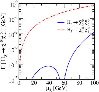
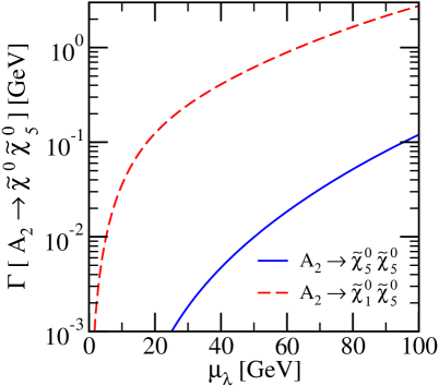
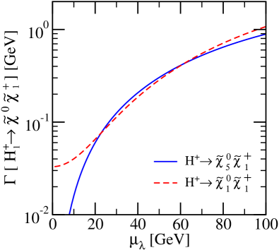
Figure 8: The decay widths for $H_{3}\to\tilde{\chi}_{1,\,5}^{0}\tilde{\chi}_{5}^{0}$ (upper left), $A_{2}\to\tilde{\chi}_{1,\,5}^{0}\tilde{\chi}_{5}^{0}$ (upper right) and $H^{\pm}\to\tilde{\chi}_{1}^{\pm}\tilde{\chi}_{1,\,5}^{0}$ (lower) for the parameter set $\mathbb{P}$[Fig.1] and maximal mixing. For the purposes of example, the Higgs mass parameter $M_{A}$ is set to $2\mu/\sin 2\beta$.

5 Summary and Conclusions

In this study, we have investigated the neutralino sector of the NMSSM, suggested by many GUT and superstring models. Moreover, this model attempts to explain the $\mu$-problem of the MSSM by introducing a new iso–singlet Higgs superfield, $\hat{S}$, the scalar component of which acquires a non-zero vacuum expectation value.

We have given expressions for the new $5\times 5$ neutralino mass matrices and mixing matrices and we have presented, besides the numerical analyses, approximate analytical solutions for the neutralino masses and mixings which provide a nice insight into the structure of the spectrum and the mass hierarchies in case of small couplings between the MSSM and the new iso–singlet.

The renormalization group flow of the parameters $\lambda$ and $\kappa$ from the GUT scale down to the electroweak scale gives rise to strong upper bounds on their values at the electroweak scale, where small $\kappa$ is favored. The qualitative features of the neutralino masses are dependent on how strongly the PQ symmetry of the model is broken by non-zero $\kappa$ values; this is quite accurately described by the approximate analytical solutions.

If the PQ symmetry is slightly broken for small $\kappa$, the qualitative pattern for the particle spectrum remains intact, except that the lightest singlino-dominant neutralino acquires a mass of the order of the electroweak scale. Thus the model contains four MSSM–type heavy gaugino/higgsino dominant states and one light singlino dominant state. Since the couplings to the $Z$ boson can be very much reduced, the NMSSM with a slightly broken PQ symmetry constitutes a valid scenario.

In contrast, a strongly broken PQ symmetry, though disfavored by the flow of the couplings from the GUT scale down to the electroweak scale, could provide an extra moderately heavy neutralino state, which is only weakly coupled to the $Z$ and (s)fermions. Such decoupled scenarios would be more difficult to distinguish the NMSSM from the MSSM.

Acknowledgments

The work of S.Y.C. was supported in part by the Korea Research Foundation Grant (KRF-2002-070-C00022) and in part by KOSEF through CHEP at Kyungpook National University.

Appendix: The small–mixing approximation

The $5\times 5$ neutralino mass matrix of Eq.(14) in general cannot be diagonalized analytically to derive the physical neutralino masses. However, simple analytical expressions for masses and mixing parameters can be found by making use of approximations for small doublet–singlet mixing which is theoretically very well motivated.

To construct this approximate solution in the neutralino sector, we treat the doublet–singlet mixing parameter $\mu_{\lambda}\ll M_{i},\mu$, together with the $Z$–boson mass $m_{Z}$, as small parameters of generic size $\varepsilon\ll 1$ in units of the typical SUSY masses. Then, as long as these SUSY masses are not as small as $\mu_{\lambda}$, we observe a hierarchical structure in the neutralino mass matrix of the form:

$${\mathcal{H}}=\left(\begin{array}[]{cc}A&X\\ X^{T}&B\end{array}\right)$$ (168)

where $A$ is a $4\times 4$ matrix incorporating elements of the order of the large SUSY scale, $B$ is a scalar and $X$ is a 4-component vector of order $\varepsilon$.

Performing an auxiliary orthogonal transformation $O$ defined by the matrix,

$$O=\left(\begin{array}[]{cc}11_{4\times 4}-\frac{1}{2}\,\Omega\Omega^{T}&\Omega\\[5.69054pt] -\Omega^{T}&1-\frac{1}{2}\,\Omega^{T}\Omega\end{array}\right)$$ (171)

with the mixing column vector $\Omega=[A-B]^{-1}X$, the mass matrix takes block diagonal form, accurate to order $\varepsilon^{2}$:

$$O{\mathcal{H}}\,O^{T} = \left(\begin{array}[]{cc}A+\Delta_{A}&0\\[2.84526pt] 0&B+\Delta_{B}\end{array}\right)$$ (174)

where

$$\Delta_{A}=\frac{1}{2}\left\{{[A-B]}^{-1},\,XX^{T}\right\}$$

$$\Delta_{B}=-X^{T}{[A-B]}^{-1}X$$ (175)

Both $\Delta$’s are of order $\varepsilon^{2}$. If $A$ is diagonal, only the diagonal elements of $\Delta_{A}$ need be kept as re–diagonalization would change the mass matrix (174) and the orthogonal matrix (171) only beyond the order considered in the systematic expansion. We note that the correction terms satisfy the simple sum rule ${\rm Tr}{\Delta_{A}}+\Delta_{B}=0$.

If $B$ is also as small as the elements of the low vector  $X$, the mixing column vector $\Omega=A^{-1}X$ and the correction terms $\Delta_{A}$ and $\Delta_{B}$ are further simplified to be

$$\Delta_{A}=\frac{1}{2}\left\{A^{-1},\,XX^{T}\right\}\ \ {\rm and}\ \ \Delta_{B}=-X^{T}A^{-1}X$$ (176)

On the contrary, if $B$ is much larger than the other parameters, the mixing column vector $\Omega=-X/B$ and the correction terms take the following simple form

$$\Delta_{A}=-XX^{T}/B,\qquad\Delta_{B}=X^{T}X/B$$ (177)

Both these approximations have been used in the derivation of all the mass and mixing formulae discussed earlier in the report.

The diagonalization of the mass matrix ${\cal M}_{5}$,

$${\cal M}_{5}=\left(\begin{array}[]{cc}{\cal M}&X\\ X^{T}&\tilde{m}_{5}\end{array}\right)$$ (180)

with ${\cal M}$ being the $4\times 4$ MSSM mass sub–matrix, makes use of the block–diagonalization method in the following way:

(1) In the first step ${\cal M}$ is diagonalized by applying the well–elaborated MSSM procedure

$${\cal M}^{D}=V{\cal M}V^{T}$$ (181)

generating the eigenvalues ${\cal M}^{D}={\rm diag}\left[\tilde{m}_{1},\ldots,\tilde{m}_{4}\right]$.

(2) The ensuing $5\times 5$ matrix can subsequently be block–diagonalized as worked out above by applying the orthogonal transformation in Eq.(171) with

$$\Omega=V\,\Gamma\;\;:\;\;\Gamma=V^{T}\left({\cal M}^{D}-\tilde{m}_{5}\right)^{-1}VX=\left({\cal M}-\tilde{m}_{5}\right)^{-1}X$$ (182)

Note that $\Gamma$ is of order $\varepsilon$ – quantum mechanically enhanced however if mass differences $|\tilde{m}_{i}-\tilde{m}_{5}|$ are, accidentally, small.

(3) The block–diagonalization affects the upper left diagonalized $4\times 4$ submatrix ${\cal M}^{D}$ only beyond second order and likewise the orthogonal matrix $V^{5}$ beyond the second and first order considered, respectively, for on– and off–diagonal elements. As a result, we obtain the final diagonal form of the mass matrix as

$${\cal M}^{D}_{5}\approx V^{5}{\cal M}_{5}V^{5T}$$ (183)

with

$$V^{5}\,\approx\,\left(\begin{array}[]{cc}11_{4\times 4}-\frac{1}{2}(V\Gamma)(V\Gamma)^{T}&(V\Gamma)\\[5.69054pt] -(V\Gamma)^{T}&1-\frac{1}{2}(V\Gamma)^{T}(V\Gamma)\end{array}\right)\,\left(\begin{array}[]{cc}V&0\\[5.69054pt] 0&11_{1\times 1}\end{array}\right)$$ (188)

in obvious notation. While the right-most part solves the MSSM diagonalization, the left-most part diagonalizes the NMSSM under the assumption of small doublet–singlet mixing.

References

- [1] P. Fayet, Phys. Lett. B 64 (1976) 159.
- [2] H.P. Nilles, Phys. Rept. 110 (1984) 1; H.E. Haber and G.L. Kane, Phys. Rept. 117 (1985) 75.
- [3] P. Fayet, Nucl. Phys. B 90 (1975) 104; M. Drees, Int. J. Mod. Phys. A 4 (1989) 3635; J. Ellis, J.F. Gunion, H. Haber, L. Roszkowski and F. Zwirner, Phys. Rev. D 39 (1989) 844, and other references quoted therein.
- [4] D.J. Miller, R. Nevzorov and P.M. Zerwas, Nucl. Phys. B 681 (2004) 3 [hep-ph/0304049].
- [5] U. Ellwanger, J.F. Gunion and C. Hugonie: NMHDECAY [hep–ph/0406215].
- [6] S.A. Abel, S. Sarkar and P.L. White, Nucl. Phys. B 454 (1995) 663; S.A. Abel, Nucl. Phys. B 480 (1996) 55; C. Panagiotakopoulos and K. Tamvakis, Phys. Lett. B 446 (1999) 224; Phys. Lett. B 469 (1999) 145; A. Dedes, C. Hugonie, S. Moretti and K. Tamvakis, Phys. Rev. D 63 (2001) 055009; C. Panagiotakopoulos and A. Pilaftsis, Phys. Rev. D 63 (2001) 055003;
- [7] M. Dine, W. Fischler and M. Srednicki, Phys. Lett. B 104 (1981) 199; H.P. Nilles, M. Srednicki and D. Wyler, Phys. Lett. B 120 (1983) 346; J.M. Frere, D.R. Jones and S. Raby, Nucl. Phys. B 222 (1983) 11; J.P. Derendinger and C.A. Savoy, Nucl. Phys. B 237 (1984) 307; A.I. Veselov, M.I. Vysotsky and K.A. Ter-Martirosian, Sov. Phys. JETP 63 (1986) 489 [Zh. Eksp. Teor. Fiz. 90 (1986) 838]; R.B. Nevzorov and M.A. Trusov, J. Exp. Theor. Phys. 91 (2000) 1079 [Zh. Eksp. Teor. Fiz. 91 (2000) 1251], [hep-ph/0106351].
- [8] F. Franke, H. Fraas and A. Bartl, Phys. Lett. B 336 (1994) 415; U. Ellwanger, M. Rausch de Traubenberg and C.A. Savoy, Phys. Lett. B 315 (1993) 331; Nucl. Phys. B 492 (1997) 21; S.F. King and P.L. White, Phys. Rev. D 52 (1995) 4183; F. Franke and H. Fraas, Z. Phys. C 72 (1996) 309; Int. J. Mod. Phys. A 12 (1997) 479; B. Ananthanarayan and P.N. Pandita, Int. J. Mod. Phys. A 12 (1997) 2321; S.P. Martin, Phys. Rev. D 62 (2000) 095008; M. Bastero–Gil, C. Hugonie, S.F. King, D.P. Roy and S. Vempati, Phys. Lett. B 489 (2000) 359; U. Ellwanger and C. Hugonie, Eur. Phys. J. C 25 (2002) 297; F. Franke and S. Hesselbach, Phys. Lett. B 526 (2002) 370; U. Ellwanger, J.F. Gunion, C. Hugonie and S. Moretti, hep-ph/0305109.
- [9] U. Ellwanger and C. Hugonie, Eur. Phys. J. C 5 (1998) 723; 13 (2000) 681.
- [10] ATLAS Technical Proposal, CERN/LHCC/94-43, LHCC/P2 (1994); CMS Technical Proposal, CERN/LHCC/94–38, LHCC/P1 (1994).
- [11] R.D. Heuer, D.J. Miller, F. Richard and P. Zerwas (eds.), TESLA: Technical Design Report (Part 3), DESY 01-011, hep-ph/0106315; American LC Working Group, T. Abe et al., SLAC-R-570 (2001), hep-ex/0106055-58; ACFA LC Working Group, K. Abe et al., KEK-REPORT-2001-11, hep-ex/0109166; CLIC Study Team, R.W. Assman et al., CERN-2000-008.
- [12] A. Stephan, Phys. Lett. B 411 (1997) 97; Phys. Rev. D 58 (1998) 035011; B.A. Dobrescu and K.T. Matchev, JHEP 0009 (2000) 031; D.J. Miller and R. Nevzorov, hep–ph/0309143; A. Menon, D.E. Morrissey and C.E.M. Wagner, hep–ph/0404184.
- [13] S.Y. Choi, J. Kalinowski, G. Moortgat-Pick and P.M. Zerwas, Eur. Phys. J. C 22 (2001) 563; 23 (2002) 769.
- [14] S.Y. Choi, A. Djouadi, M. Guchait, J. Kalinowski, H.S. Song and P.M. Zerwas, Eur. Phys. J. C 14, 535 (2000).
- [15] S.Y. Choi, H.S. Song and W.Y. Song, Phys. Rev. D 61 (2000) 075004.