LORENTZ-NONINVARIANT NEUTRINO OSCILLATIONS:
MODEL AND PREDICTIONS

Abstract

We present a three-parameter neutrino-oscillation model for three flavors of massless neutrinos with Fermi-point splitting and tri-maximal mixing angles. One of these parameters is the T–violating phase $\epsilon$, for which the experimental results from K2K and KamLAND appear to favor a nonzero value. In this article, we give further model predictions for neutrino oscillations. Upcoming experiments will be able to test this simple model and the general idea of Fermi-point splitting. Possible implications for proposed experiments and neutrino factories are also discussed.

PACS numbers: 14.60.St, 11.30.Cp, 73.43.Nq

1 Introduction

Several experiments of the last few years [SuperK1998][SNO2003] have presented (indirect) evidence for neutrino oscillations over a travel distance $L\gtrsim 100\,\mathrm{km}$. No evidence for neutrino oscillations has been seen at $L\lesssim 1\,\mathrm{km}$.[CHOOZ2002, PaloVerde2001]

The standard explanation for neutrino oscillations invokes the mass-difference mechanism; see, e.g., Refs. GribovPontecorvo–Lipkin for a selection of research papers and Refs. Bargeretal–McKeownVogel for two recent reviews. Another possibility, based on an analogy with condensed-matter physics,[VolovikBook] is the Fermi-point-splitting mechanism suggested by Volovik and the present author. The idea is that a quantum phase transition could give rise to Lorentz noninvariance and CPT violation via the splitting of a multiply degenerate Fermi point; see Ref. KlinkhamerVolovikJETPL for an introduction and Ref. KlinkhamerVolovik for details. Regardless of the origin, it may be worthwhile to study modifications of the neutrino dispersion law other than mass terms, Fermi-point splitting being one of the simplest such modifications.

A first comparison of this Lorentz-noninvariant mechanism for neutrino oscillations with the current experimental data from K2K and KamLAND (with additional input from Super–Kamiokande) was presented in Ref. KlinkhamerJETPL. Rough agreement was found for a two-parameter model with tri-maximal mixing angles. The comparison with the experimental data indicated a scale of the order of $10^{-12}\;{\rm eV}$ for the Fermi-point splitting of the neutrinos and showed a preference for a nonzero value of the T–violating phase $\epsilon$. (Note that this phase $\epsilon$ differs, in general, from the one associated with mass terms, which will be denoted by $\delta$ in the following.)

In this article, we discuss in detail a three-parameter model with tri-maximal mixing, which is a direct extension of the previous two-parameter model. We, then, try to make specific predictions for possible future experiments, e.g., MINOS,[MINOS1998, MINOS2003] ICARUS,[ICARUS] OPERA,[OPERA] T2K,[JPARCSK2001, H2B2001] NO$\nu$A,[NOvA] BNL–$\nu$,[BNL2002] beta beams,[Zucchelli] neutrino factories,[Geer1997, Blondel2004] and reactor experiments.[Whitepaper]

Let us emphasize, right from the start, that the model considered is only one of the simplest possible. It could very well be that the mixing angles are not tri-maximal and that there are additional mass-difference effects. However, with both mass differences and Fermi-point splittings present, there is a multitude of mixing angles and phases to consider. For this reason, we study in the present article only the simple Fermi-point-splitting model with tri-maximal mixing and zero mass differences, which, at least, makes the predictions unambiguous. Also, it is not our goal to give the best possible fit to all the existing experimental data on neutrino oscillations but, rather, to look for qualitatively new effects (e.g., T and CPT violation).

The outline of this article is as follows. In Section 2, we discuss the general form of the dispersion law with Fermi-point splitting. In Section 3, we present a simple three-parameter model for three flavors of massless neutrinos with Fermi-point splitting and tri-maximal mixing angles. In Section 4, we calculate the neutrino-oscillation probabilities for the model considered. In Section 5, we obtain preliminary values for the three parameters of the model and make both general and specific predictions (the latter are for MINOS and T2K in particular). In Section LABEL:sec:outlook, finally, we sketch a few scenarios of what future neutrino-oscillation experiments could tell us about the relevance of the Fermi-point-splitting model.

2 Fermi-Point Splitting

In the limit of vanishing Yukawa couplings, the Standard Model fermions are massless Weyl fermions, which have the following dispersion law:

$$\bigl{(}E_{a,f}({\bf p})\bigr{)}^{2} = \Bigl{(}\,c\,|{\bf p}|+b_{0a}^{(f)}\Bigr{)}^{2}\,,$$ (1)

for three-momentum ${\bf p}$, velocity of light $c$, and parameters $b_{0a}^{(f)}=0$. Here, $a$ labels the sixteen types of massless left-handed Weyl fermions in the Standard Model (with a hypothetical left-handed antineutrino included) and $f$ distinguishes the three known fermion families. For right-handed Weyl fermions and the same parameters, the plus sign inside the square on the right-hand side of Eq. (1) becomes a minus sign; cf. Refs. KlinkhamerVolovik,CK97.

The Weyl fermions of the original Standard Model have all $b_{0a}^{(f)}$ in Eq. (1) vanishing, which makes for a multiply degenerate Fermi point ${\bf p}={\bf 0}$. [ Fermi points (gap nodes) ${\bf p}_{n}$ are points in three-dimensional momentum space at which the energy spectrum $E({\bf p})$ of the fermionic quasi-particle has a zero, i.e., $E({\bf p}_{n})=0$.]

Negative parameters $b_{0a}^{(f)}$ in the dispersion law (1) split this multiply degenerate Fermi point into Fermi surfaces. [ Fermi surfaces $S_{n}$ are two-dimensional surfaces in three-dimensional momentum space on which the energy spectrum $E({\bf p})$ is zero, i.e., $E({\bf p})=0$ for all ${\bf p}\in S_{n}$.] Positive parameters $b_{0a}^{(f)}$ make the respective Fermi points disappear altogether, the absolute value of the energy being larger than zero for all momenta. See Refs. KlinkhamerVolovikJETPL,KlinkhamerVolovik for a discussion of the quantum phase transition associated with Fermi-point splitting. Note that the dispersion law (1) with nonzero parameters $b_{0a}^{(f)}$ selects a class of preferred reference frames; cf. Refs. CK97–CarrollFieldJackiw.

Possible effects of Fermi-point splitting include neutrino oscillations,[KlinkhamerVolovik, KlinkhamerJETPL] as long as the neutrinos are not too much affected by the mechanism of mass generation. The hope is that massless (or nearly massless) neutrinos provide a window on “new physics,” with Lorentz invariance perhaps as emergent phenomenon.[VolovikBook] Let us, then, turn to the phenomenology of massless neutrinos with Fermi-point splittings.

We start from the observation that the Fermi-point splittings of the Standard Model fermions may have a special pattern tracing back to the underlying physics, just as happens for the so-called $\alpha$–phase of spin-triplet pairing in superconductors.[KlinkhamerVolovikJETPL, KlinkhamerVolovik] As an example, consider the following factorized Ansatz[KlinkhamerVolovik] for the timelike splittings of Fermi points:

$$b_{0a}^{(f)}=Y_{a}\;b_{0}^{(f)}\,,$$ (2)

for $a=1,\ldots,16$ and $f=1,2,3$. Given the hypercharge values $Y_{a}$ of the Standard Model fermions, there is only one arbitrary energy scale $b_{0}$ per family.

The motivation of the particular choice (2) is that the induced electromagnetic Chern–Simons-like term cancels out exactly (the result is directly related to the absence of perturbative gauge anomalies in the Standard Model). This cancellation mechanism allows for $b_{0a}^{(f)}$ values larger than the experimental upper limit on the Chern–Simons energy scale,[CarrollFieldJackiw] which is of the order of $10^{-33}\;{\rm eV}$. Other radiative effects from nonzero $b_{0a}^{(f)}$ remain to be calculated; cf. Ref. MocioiuPospelov.

The dispersion law of a massless left-handed neutrino (hypercharge $Y_{\nu_{L}}=-1$) is now given by

$$\bigl{(}E_{\nu_{L},f}({\bf p})\bigr{)}^{2} = \Bigl{(}\,c\,|{\bf p}|-b_{0}^{(f)}\,\Bigr{)}^{2}\,,$$ (3)

with $f=1,2,3,$ for three neutrinos. The corresponding right-handed antineutrino is taken to have the following dispersion law:

$$\bigl{(}E_{\bar{\nu}_{R},f}({\bf p})\bigr{)}^{2} = \Bigl{(}\,c\,|{\bf p}|+\sigma\,b_{0}^{(f)}\,\Bigr{)}^{2}\,,$$ (4)

with $\sigma=\pm 1$. Starting from Dirac fermions, the natural choice would be $\sigma=-1$; cf. Refs. KlinkhamerVolovik,CK97. But, in the absence of a definitive mechanism for the Fermi-point splitting, we keep both possibilities open. We do not consider the further generalization of having $\sigma$ in Eq. (4) depend on the family index $f$.

The dispersion laws (3) and (4) can be considered independently of the particular splitting pattern for the other Standard Model fermions, of which Eq. (2) is only one example. The parameters $b_{0}^{(f)}$ in these neutrino dispersion laws act as chemical potentials. This may be compared to the role of rest mass in a generalized dispersion law:

$$\bigl{(}E({\bf p})\bigr{)}^{2}=\Bigl{(}\,c\,|{\bf p}|\pm b_{0}\,\Bigr{)}^{2}+m^{2}\,c^{4}\sim\left(\,c\,|{\bf p}|\pm b_{0}+\frac{m^{2}\,c^{4}}{2\,c\,|{\bf p}|}\,\right)^{2}\!,$$ (5)

for $|{\bf p}|\gg\max\,\left(|b_{0}|/c,mc\right)$. The energy change from a nonzero $b_{0}$ always dominates the effect from $mc^{2}$ for large enough momenta $|{\bf p}|$. In order to search for Fermi-point splitting, it is, therefore, preferable to use neutrino beams with the highest possible energy.

3 Neutrino Model

Now define three flavor states $|A\rangle,|B\rangle,|C\rangle$ in terms of the left-handed propagation states $|1\rangle,|2\rangle,|3\rangle$, which have dispersion law (3) with parameters $b_{0}^{(f)}$, $f=1,2,3$. With a unitary $3\times 3$ matrix $U$, the relation between these states is

$$\left(\begin{array}[]{c}|A\rangle\\ |B\rangle\\ |C\rangle\end{array}\right) = \;U\;\left(\begin{array}[]{c}|1\rangle\\ |2\rangle\\ |3\rangle\end{array}\right)\,.$$ (12)

The matrix $U$ can be parametrized[Bargeretal, McKeownVogel] by three mixing angles, $\chi_{13},\chi_{21},\chi_{32}\in[0,\pi/2]$, and one phase, $\epsilon\in[0,2\pi]$:

$$U\equiv\left(\begin{array}[]{ccc}1&0&0\\ 0&c_{32}&s_{32}\\ 0&-s_{32}&c_{32}\end{array}\right)\cdot\left(\begin{array}[]{ccc}c_{13}&0&\;+s_{13}\,e^{+i\epsilon}\\ 0&1&0\\ -s_{13}\,e^{-i\epsilon}&0&c_{13}\end{array}\right)\cdot\left(\begin{array}[]{ccc}c_{21}&s_{21}&0\\ -s_{21}&c_{21}&0\\ 0&0&1\end{array}\right)\,,$$ (13)

using the standard notation $s_{ij}$ and $c_{ij}$ for $\sin\chi_{ij}$ and $\cos\chi_{ij}$.

In this article, we generalize the Ansatz of Ref. KlinkhamerJETPL by allowing for unequal ($r\neq 1$) energy steps $\Delta b_{0}^{(ji)}\equiv b_{0}^{(j)}-b_{0}^{(i)}$ between the first and second families ($i,j=1,2$) and between the second and third ($i,j=2,3$). Specifically, we introduce the parameters

$$B_{0}\equiv\Delta b_{0}^{(21)}\equiv b_{0}^{(2)}-b_{0}^{(1)}\,,\quad r\equiv\Delta b_{0}^{(32)}/\Delta b_{0}^{(21)}\equiv\bigl{(}\,b_{0}^{(3)}-b_{0}^{(2)}\bigr{)}/B_{0}\,,$$ (14)

which are assumed to be nonnegative. The overall energy scale of the three parameters $b_{0}^{(f)}$ is left unspecified. Note, however, that positive $b_{0}^{(f)}$ in Eq. (3) give rise to Fermi surfaces, which may or may not be topologically protected; cf. Refs. VolovikBook,KlinkhamerVolovik.

The mixing angles are again taken to be tri-maximal,[KlinkhamerJETPL]

$$\chi_{13}=\arctan\sqrt{1/2}\approx\pi/5\,,\quad\chi_{21}=\chi_{32}=\arctan 1=\pi/4\,.$$ (15)

These particular values maximize, for given phase $\epsilon$, the following T–violation (CP–nonconservation) measure:

$$J\equiv\frac{1}{8}\,\cos\chi_{13}\,\sin 2\chi_{13}\,\sin 2\chi_{21}\,\sin 2\chi_{32}\,\sin\epsilon\,,$$ (16)

which is independent of phase conventions.[Jarlskog] For this reason, we prefer to use the values (15) rather than the ad hoc values $\chi_{13}=\chi_{21}=\chi_{32}=\pi/4$.

In one of the first articles on neutrino oscillations, Bilenky and Pontecorvo[BilenkyPontecorvo1976] emphasized the essential difference between leptons and quarks, where the latter have quantum numbers which are conserved by the strong interactions. They argued that, for two flavors, the only natural value of the neutrino mixing angle $\chi$ is $0$ or $\pi/4$. But, at this moment, we do not know of a physical mechanism which convincingly explains the tri-maximal values (15) and we simply use these values as a working hypothesis.

In short, the model (12)–(15), for dispersion law (3), has three parameters: the basic energy-difference scale $B_{0}\equiv\Delta b_{0}^{(21)}$, the ratio $r$ of the consecutive energy steps $\Delta b_{0}^{(21)}$ and $\Delta b_{0}^{(32)}$, and the T–violating phase $\epsilon$. This model will be called the “simple” Fermi-point-splitting model in the following (a more general Fermi-point-splitting model would have arbitrary mixing angles).

4 Neutrino-Oscillation Probabilities

The calculation of neutrino-oscillation probabilities is technically straightforward but conceptually rather subtle; cf. Refs Kayser–Lipkin. It may be the simplest to consider a stationary mono-energetic beam of left-handed neutrinos originating from a specified interaction region and propagating over a distance $L$ to an appropriate detector. That is, the neutrinos start out with a definite flavor (here, labeled $A,B,C$) and have a spread in their momenta (from the finite size of the interaction region and the Heisenberg uncertainty principle, $\Delta x_{m}\;\Delta p_{n}\geq\delta_{mn}\;\hbar/2\,$).

For dispersion law (3) and large enough neutrino energy ($E_{\nu}\geq\mathrm{max}\;[\,b_{0}^{(f)}\,]\,$), the tri-maximal model (12)–(15) gives the following neutrino-oscillation probabilities:

$$P(A\rightarrow B,\,\epsilon) = \frac{2}{9}\,\Bigl{[}\,\,\sin^{2}\frac{\Delta_{21}}{2}+\bigl{(}1+{\sqrt{3}}\,c_{\epsilon}\bigr{)}\,\sin^{2}\frac{\Delta_{31}}{2}+\bigl{(}1-{\sqrt{3}}\,c_{\epsilon}\bigr{)}\,\sin^{2}\frac{\Delta_{32}}{2}$$ (17a)

$$-(1/2)\,\sqrt{3}\;s_{\epsilon}\,\bigl{(}\sin{\Delta_{21}}-\sin{\Delta_{31}}+\sin{\Delta_{32}}\bigr{)}\,\Bigr{]}\,,$$

$$P(A\rightarrow C,\,\epsilon) = \frac{2}{9}\,\Bigl{[}\,\,\sin^{2}\frac{\Delta_{21}}{2}+\bigl{(}1-{\sqrt{3}}\,c_{\epsilon}\bigr{)}\,\sin^{2}\frac{\Delta_{31}}{2}+\bigl{(}1+{\sqrt{3}}\,c_{\epsilon}\bigr{)}\,\sin^{2}\frac{\Delta_{32}}{2}$$ (17b)

$$+(1/2)\,\sqrt{3}\;s_{\epsilon}\,\bigl{(}\sin{\Delta_{21}}-\sin{\Delta_{31}}+\sin{\Delta_{32}}\bigr{)}\,\Bigr{]}\,,$$

$$P(A\rightarrow A,\,\epsilon) = 1-P(A\rightarrow B,\,\epsilon)-P(A\rightarrow C,\,\epsilon)\,,$$ (17c)

$$P(B\rightarrow C,\,\epsilon) = \frac{2}{9}\,\Bigl{[}\;(1/2)\left(3\,{s_{\epsilon}}^{2}-1\right)\,\sin^{2}\frac{\Delta_{21}}{2}+\,\sin^{2}\frac{\Delta_{31}}{2}+\,\sin^{2}\frac{\Delta_{32}}{2}$$ (17d)

$$-(1/2)\,\sqrt{3}\;s_{\epsilon}\,\bigl{(}\sin{\Delta_{21}}-\sin{\Delta_{31}}+\sin{\Delta_{32}}\bigr{)}\,\Bigr{]}\,,$$

$$P(B\rightarrow A,\,\epsilon) = \frac{2}{9}\,\Bigl{[}\,\,\sin^{2}\frac{\Delta_{21}}{2}+\bigl{(}1+{\sqrt{3}}\,c_{\epsilon}\bigr{)}\,\sin^{2}\frac{\Delta_{31}}{2}+\bigl{(}1-{\sqrt{3}}\,c_{\epsilon}\bigr{)}\,\sin^{2}\frac{\Delta_{32}}{2}$$ (17e)

$$+(1/2)\,\sqrt{3}\;s_{\epsilon}\,\bigl{(}\sin{\Delta_{21}}-\sin{\Delta_{31}}+\sin{\Delta_{32}}\bigr{)}\,\Bigr{]}\,,$$

$$P(B\rightarrow B,\,\epsilon) = 1-P(B\rightarrow C,\,\epsilon)-P(B\rightarrow A,\,\epsilon)\,,$$ (17f)

$$P(C\rightarrow A,\,\epsilon) = \frac{2}{9}\,\Bigl{[}\,\,\sin^{2}\frac{\Delta_{21}}{2}+\bigl{(}1-{\sqrt{3}}\,c_{\epsilon}\bigr{)}\,\sin^{2}\frac{\Delta_{31}}{2}+\bigl{(}1+{\sqrt{3}}\,c_{\epsilon}\bigr{)}\,\sin^{2}\frac{\Delta_{32}}{2}$$ (17g)

$$-(1/2)\,\sqrt{3}\;s_{\epsilon}\,\bigl{(}\sin{\Delta_{21}}-\sin{\Delta_{31}}+\sin{\Delta_{32}}\bigr{)}\,\Bigr{]}\,,$$

$$P(C\rightarrow B,\,\epsilon) = \frac{2}{9}\,\Bigl{[}\;(1/2)\left(3\,{s_{\epsilon}}^{2}-1\right)\,\sin^{2}\frac{\Delta_{21}}{2}+\,\sin^{2}\frac{\Delta_{31}}{2}+\,\sin^{2}\frac{\Delta_{32}}{2}$$ (17h)

$$+(1/2)\,\sqrt{3}\;s_{\epsilon}\,\bigl{(}\sin{\Delta_{21}}-\sin{\Delta_{31}}+\sin{\Delta_{32}}\bigr{)}\,\Bigr{]}\,,$$

$$P(C\rightarrow C,\,\epsilon) = 1-P(C\rightarrow A,\,\epsilon)-P(C\rightarrow B,\,\epsilon)\,,$$ (17i)

with $s_{\epsilon}\equiv\sin\epsilon$, $c_{\epsilon}\equiv\cos\epsilon$, and

$$\Delta_{fg} \equiv \left(b_{0}^{(f)}-b_{0}^{(g)}\right)\frac{L}{\hbar\,c}\>.$$ (18)

Specifically, the Fermi-point-splitting Ansatz has

$$\Delta_{21}=2\pi\,l\,,\quad\Delta_{32}=2\pi\,l\,r\,,\quad\Delta_{31}=2\pi\,l\,(1+r)\,,$$ (19)

in terms of the dimensionless distance

$$l\equiv B_{0}\,L/(h\,c)$$ (20)

and parameters $B_{0}$ and $r$ from Eq. (14).

The probabilities for right-handed antineutrinos (flavors $X,Y\in\{A,B,C\}$) are given by

$$P(\bar{X}\rightarrow\bar{Y},\,\epsilon)=P(X\rightarrow Y,\,\sigma\epsilon)\,,$$ (21)

as follows by changing $\epsilon\rightarrow-\epsilon$ and $B_{0}\rightarrow-\sigma B_{0}$ in Eqs. (17a)–(17i), where the latter transformation corresponds to the change from (3) to (4) with $\sigma=\pm 1$. Note that the survival probability of right-handed antineutrinos equals that of left-handed neutrinos,

$$P(\bar{X}\rightarrow\bar{X},\,\epsilon) = P(X\rightarrow X,\,\epsilon)\,,$$ (22)

independent of the choice of $\sigma$ in the antineutrino dispersion law (4).

The time-reversal asymmetry parameter for oscillation probabilities between $X$–type and $Y$–type neutrinos ($X\neq Y$) is defined by

$$a^{\mathrm{(T)}}_{XY}\equiv\frac{P(Y\rightarrow X,\,\epsilon)-P(X\rightarrow Y,\,\epsilon)}{P(Y\rightarrow X,\,\epsilon)+P(X\rightarrow Y,\,\epsilon)}\,.$$ (23)

For model probabilities (17), this asymmetry parameter is proportional to $\sin\epsilon$. The corresponding CP asymmetry parameter is given by

$$a^{\mathrm{(CP)}}_{XY}\equiv\frac{P(\bar{X}\rightarrow\bar{Y},\,\epsilon)-P(X\rightarrow Y,\,\epsilon)}{P(\bar{X}\rightarrow\bar{Y},\,\epsilon)+P(X\rightarrow Y,\,\epsilon)}\,.$$ (24)

For model probabilities (17) and (21), this last asymmetry parameter vanishes for $\sigma=+1$ and equals $a^{\mathrm{(T)}}_{XY}$ for $\sigma=-1$. In other words, the oscillation probabilities (17) and (21) of the neutrino model with $\sin\epsilon\neq 0$ violate T and CPT for the case of $\sigma=+1$ and violate T and CP (but keep CPT invariance intact) for the case of $\sigma=-1$. In the absence of a definitive theory, it is up to experiment to decide between the options $\sigma=\pm 1$.

For completeness, we recall that the standard mass-difference mechanism gives the following oscillation probabilities[Bargeretal, McKeownVogel] for fixed ratio $L/E_{\nu}$ and small enough mass-square difference $|\Delta m^{2}_{21}|\equiv|m^{2}_{2}-m^{2}_{1}|$:

$$P_{\mathrm{mass-oscill}}(\nu_{\mu}\rightarrow\nu_{e})\sim\sin^{2}(2\,\underline{\theta}_{\,13})\,\sin^{2}\underline{\theta}_{\,32}\,\sin^{2}\Omega_{32}\,,$$ (25a)

$$P_{\mathrm{mass-oscill}}(\nu_{\mu}\rightarrow\nu_{\tau})\sim\cos^{4}\underline{\theta}_{\,13}\,\sin^{2}(2\,\underline{\theta}_{\,32})\,\sin^{2}\Omega_{32}\,,$$ (25b)

with $\Omega_{ij}\equiv\Delta m^{2}_{ij}\,c^{4}\,L\,/\,(4\,E_{\nu}\,\hbar\,c)$. The mixing angles $\underline{\theta}_{\,ij}$ are associated with the mass terms in the action and are, in general, different from those defined by Eqs. (12)–(13); cf. Ref. ColemanGlashow. In fact, the underlined parameters refer to the pure mass-difference model with all Fermi-point-splittings strictly zero. Observe that the T–violating phase $\underline{\delta}$ has dropped out in Eqs. (25ab) because of the limit $\Delta m^{2}_{21}\to 0$.

For $|\Delta m^{2}_{32}|\gg|\Delta m^{2}_{21}|$ and considering $L$ to be an average distance, one has effectively

$$P_{\mathrm{mass-oscill}}(\nu_{e}\rightarrow\nu_{e})=P_{\mathrm{mass-oscill}}(\bar{\nu}_{e}\rightarrow\bar{\nu}_{e})$$

$$\sim 1-(1/2)\,\sin^{2}(2\,\underline{\theta}_{\,13})\,-\cos^{4}\underline{\theta}_{\,13}\,\sin^{2}(2\,\underline{\theta}_{\,21})\,\sin^{2}\Omega_{21}\,,$$ (26)

with the $\Omega_{13}$ and $\Omega_{32}$ terms averaged over.

The expressions (25ab) have been used to analyze the data from K2K[K2K2002, K2K2004] and the expression (26) for the data from KamLAND,[KamLAND2002, KamLAND2004] all three theoretical expressions being independent of the phase $\underline{\delta}$. In the next section, we will use instead the expressions (17)–(22) from the simple Fermi-point-splitting model, which are dependent on the T–violating phase $\epsilon$. But, for brevity, we will drop the explicit $\epsilon$ dependence, just writing $P(X\rightarrow Y)$ and $P(\bar{X}\rightarrow\bar{Y})$.

5 Model Parameters and Predictions

In order to make unambiguous predictions, we assume in the main part of this article that the neutrino mass differences are strictly zero. It could, however, be that Eqs. (3)–(4) are modified by having (small) mass-square terms on their right-hand-sides, as in Eq. (5), which possibility will be briefly discussed in Sec. LABEL:sec:outlook.

5.1 General model predictions

The most general prediction of the Fermi-point-splitting mechanism of neutrino oscillations is that the oscillation properties are essentially independent of the neutrino energies. This implies undistorted energy spectra for the reconstructed $\nu_{\mu}$ energies in, for example, the current K2K experiment[K2K2002, K2K2004] and the future MINOS experiment.[MINOS1998, MINOS2003] [As argued in Ref. KlinkhamerJETPL, the energy spectra from K2K[K2K2002] and KamLAND[KamLAND2002, KamLAND2004] are certainly suggestive of the mass-difference mechanism but do not rule out the Fermi-point-splitting mechanism yet. The same conclusion holds for the zenith-angle distributions of upward stopping or through-going muons from Super–Kamiokande (SK); cf. Fig. 39 of Ref. KajitaTotsuka2001, which appears to have a relatively large uncertainty on the calculated flux of upward through-going muons.]

Assuming that the energy splittings (18) are responsible for the neutrino-oscillation results of SK, K2K, and KamLAND (see below), another prediction[KlinkhamerJETPL] is that any reactor experiment at $L=\ell\approx 1\,\mathrm{km}$ (cf. Refs. CHOOZ2002,PaloVerde2001,Whitepaper) will have survival probabilities close to 1, at least up to an accuracy of order $(\Delta b_{0}\,\ell/\hbar c)^{2}\approx 10^{-4}$ for $|\Delta b_{0}|\approx 2\times 10^{-12}\;{\rm eV}$.

Both predictions hold, of course, only if mass-difference effects from the generalized dispersion law (5) are negligible compared to Fermi-point-splitting effects with $|\Delta b_{0}|=\mathrm{O}(10^{-12}\;{\rm eV})$. This corresponds to $|\Delta m^{2}|\lesssim 10^{-6}\,\mathrm{eV}^{2}/c^{4}$ for (anti)neutrino energies in the $\mathrm{MeV}$ range. For larger mass differences, the corresponding mixing angles may need to be small, for example $\theta_{\,13}\lesssim 0.2$ for $|\Delta m^{2}_{13}|=2\times 10^{-3}\;{\rm eV}^{2}/c^{4}$; see Refs. CHOOZ2002,PaloVerde2001. As mentioned in the preamble of this section, our model predictions will be for $\Delta m^{2}_{ij}=0$ and $\Delta b_{0}^{(ij)}\neq 0$, with mixing angles $\chi_{ij}$ defined by Eqs. (12), (13) and (15).

5.2 Preliminary parameter values

We now present model probabilities at three dimensionless distances $l$ which have ratios 250:180:735 corresponding to the baselines of the K2K, KamLAND and MINOS experiments, but, initially, we focus on the first two distances. [The dimensionless distance $l$ has been defined in Eq. (20).] In Table 5.2, model probabilities are calculated starting from an appropriate dimensionless distance $\tilde{l}$, for a fixed phase $\epsilon=\pi/4$ and different values of the parameter $r$ as defined by Eq. (14). The $\tilde{l}$ values are chosen so that the following inequality holds: $P(C\rightarrow C)\geq 65\,\%$ for $0\leq l\leq\tilde{l}$.

Fixing the ratio $r$ to the value $1/2$, Table 5.2 gives model probabilities for different values of the phase $\epsilon$. The $\epsilon$ range can be restricted to $(-\pi/2,\pi/2]$ without loss of generality, because the probabilities (17) are invariant under the combined transformations $\epsilon\rightarrow\epsilon+\pi$ and $(A,B,C)\rightarrow(A,C,B)$.

Model probabilities $(P)|^{\epsilon,r}_{l}$ for different values of the energy-splitting ratio $r$ and dimensionless distance $l$, with fixed phase $\epsilon=\pi/4$. The probabilities $P$ are calculated from Eqs. (17a)–(17i) and are given in percent, with a rounding error of $1$. The last row gives the experimental results for $(P_{\nu_{\mu}\rightarrow\nu_{\mu}},P_{\nu_{\mu}\rightarrow\nu_{e}},P_{\nu_{\mu}\rightarrow\nu_{\tau}})$ at $L=250\;\mathrm{km}$ from K2K[K2K2002, K2K2004] and for $(P_{\bar{\nu}_{e}\rightarrow\bar{\nu}_{e}})$ at $L\approx 180\;\mathrm{km}$ from KamLAND.[KamLAND2002, KamLAND2004] The relative error on these experimental numbers is of the order of $10\,\%$. Also shown are possible results for MINOS[MINOS1998] from standard mass-difference neutrino oscillations, where the values for $(P_{\nu_{\mu}\rightarrow\nu_{\mu}},P_{\nu_{\mu}\rightarrow\nu_{e}},P_{\nu_{\mu}\rightarrow\nu_{\tau}})$ are calculated from Eqs. (25ab) for $L=735\;\mathrm{km}$, $E_{\nu}=3\;{\rm GeV}$, $|\Delta m^{2}_{32}|=2\times 10^{-3}\;{\rm eV}^{2}/c^{4}$, $\sin^{2}(2\,\underline{\theta}_{\,32})=1$, and $\sin^{2}(2\,\underline{\theta}_{\,13})=0.2\,$. $\tilde{r}$ $\tilde{l}$ $\;\bigl{(}P_{C\rightarrow C},P_{C\rightarrow A},P_{C\rightarrow B}\bigr{)}\Big{|}^{\;\frac{\pi}{4},\tilde{r}}_{\;\tilde{l}}\;$ $\;\bigl{(}P_{\bar{A}\rightarrow\bar{A}}\bigr{)}\Big{|}^{\;\frac{\pi}{4},\tilde{r}}_{\;\tilde{l}\times\frac{180}{250}}$ $\;\bigl{(}P_{C\rightarrow C},P_{C\rightarrow A},P_{C\rightarrow B}\bigr{)}\Big{|}^{\;\frac{\pi}{4},\tilde{r}}_{\;\tilde{l}\times\frac{735}{250}}$  1/8  0.250 ( 75 , 6 , 19 ) ( 71 ) ( 74 ,  9 , 17 ) 1/8 0.320 ( 65 , 7 , 28 ) ( 57 ) ( 89 ,  8 ,  3 ) 1/4   0.230 ( 75 , 3 , 22 ) ( 72 ) ( 58 , 17 , 25 ) 1/4 0.260 ( 70 , 3 , 27 ) ( 65 ) ( 64 , 23 , 13 ) 1/4 0.290 ( 65 , 3 , 32 ) ( 59 ) ( 66 , 26 ,  8 ) 1/2 0.190 ( 75 , 1 , 24 ) ( 74 ) ( 27 , 29 , 44 ) 1/2 0.210 ( 70 , 1 , 29 ) ( 69 ) ( 26 , 43 , 31 ) 1/2 0.230 ( 65 , 1 , 34 ) ( 64 ) ( 25 , 56 , 19 ) 1 0.130 ( 75 , 2 , 23 ) ( 79 ) (  6 , 28 , 66 ) 1 0.145 ( 70 , 2 , 28 ) ( 74 ) (  2 , 44 , 54 ) 1 0.160 ( 65 , 2 , 33 ) ( 69 ) (  1 , 61 , 38 ) 2 0.080 ( 74 , 6 , 20 ) ( 81 ) (  5 , 27 , 68 ) 2 0.095 ( 65 , 7 , 28 ) ( 74 ) ( 10 , 40 , 50 ) – –  K2K:  ( 70 , $\leq 1$ , 29 )  KamLAND:  ( 66 )  MINOS:  ( 66? , 3? , 31? )

Model probabilities $(P)|^{\epsilon,r}_{l}$ for different values of the phase $\epsilon$ and dimensionless distance $l$, with fixed energy-splitting ratio $r=1/2$. The probabilities $P$ are calculated from Eqs. (17a)–(17i) and are given in percent, with a rounding error of $1$. For different values of $\epsilon$ and $l$, $\{X,Y,Z\}$ stands for a permutation of the basic flavors $\{A,B,C\}$. For $\epsilon=+\pi/2$, the same probabilities hold for cyclic permutations of $\{C,A,B\}$, that is, $\{X,Y,Z\}$ can be $\{C,A,B\}$, $\{A,B,C\}$, or $\{B,C,A\}$. The last line gives the experimental results from K2K and KamLAND; see Table 5.2 for further details. $\tilde{\epsilon}$ $\tilde{l}$ $\,\{X,Y,Z\}\,$ $\,\bigl{(}P_{X\rightarrow X},P_{X\rightarrow Y},P_{X\rightarrow Z}\bigr{)}\Big{|}^{\;\tilde{\epsilon},\frac{1}{2}}_{\;\tilde{l}}\,$ $\,\bigl{(}P_{\bar{Y}\rightarrow\bar{Y}}\bigr{)}\Big{|}^{\;\tilde{\epsilon},\frac{1}{2}}_{\;\tilde{l}\times\frac{180}{250}}\,$ $-\pi/4$  0.135 $\{A,C,B\}$ ( 75 ,  1 , 24 ) ( 92 ) $-\pi/4$  0.160 $\{A,C,B\}$ ( 66 ,  1 , 33 ) ( 90 ) $0$  0.135 $\{A,C,B\}$ ( 75 ,  1 , 24 ) ( 96 ) $0$  0.160 $\{A,C,B\}$ ( 66 ,  1 , 33 ) ( 94 ) $+\pi/4$  0.190 $\{C,A,B\}$ ( 75 ,  1 , 24 ) ( 74 ) $+\pi/4$  0.230 $\{C,A,B\}$ ( 65 ,  1 , 34 ) ( 64 ) $\,+\pi/2\,$  0.135 $\{C,A,B\}^{\text{cycl.}}$ ( 75 ,  9 , 16 ) ( 86 ) $\,+\pi/2\,$  0.160 $\{C,A,B\}^{\text{cycl.}}$ ( 66 , 11 , 23 ) ( 81 ) – – xxxx–  K2K:  ( 70 , $\leq 1$ , 29 )  KamLAND:  ( 66 )

The last rows of Tables 5.2 and 5.2 give the experimental results from K2K[K2K2002, K2K2004] and KamLAND.[KamLAND2002, KamLAND2004] The K2K numbers are deduced from the expected total number of events $80\pm 6$ and the observed numbers of $\nu_{\mu}$ and $\nu_{e}$ events, respectively $56$ and $1$ (background?). The latest KamLAND value for the average $\bar{\nu}_{e}$ survival probability is $0.658\pm 0.044\,{\rm(stat)}\pm 0.047\,{\rm(syst)}$.

Regarding the comparison of the model values and the K2K data in Table 5.2, recall that the normalized Poisson distribution $p(n;\mu)\equiv\exp(-\mu)\,\mu^{n}\,/n!$ gives $p(1;6)\sim 1\%$ and $p(1;3)\sim 15\%$. This suggests that the best value for $r$ is somewhere between $1/8$ and $2$. Similarly, Table 5.2 shows a preference for a value of $\epsilon$ around $\pi/4$ (or $5\pi/4$ with trivial relabelings).

The basic energy-difference scale $B_{0}$ of the model is determined by identifying the $\tilde{l}$ value of one particular row in Table 5.2 or 5.2 with the K2K baseline of $250\,\mathrm{km}$. Using Eq. (20), one has

$$B_{0}=h\,c\;\;\tilde{l}/L_{\mathrm{K2K}}=1.04\times 10^{-12}\;{\rm eV}\,\left(\frac{250\>\mathrm{km}}{L_{\mathrm{K2K}}}\right)\,\left(\frac{\tilde{l}}{0.210}\right)\,.$$ (27)

From the numbers in Tables 5.2 and 5.2, the combined K2K and KamLAND results then give the following “central values” for the parameters of the model (12)–(15):

$$B_{0}\approx 10^{-12}\;{\rm eV}\,,\quad r\approx 1/2\,,\quad\epsilon\approx\pi/4\!\pmod{\pi}\,,$$ (28)

with identifications

$$\Bigl{(}|A\rangle\,,|B\rangle\,,|C\rangle\Bigr{)} = \left.\Bigl{(}|\nu_{e}\rangle\,,|\nu_{\tau}\rangle\,,|\nu_{\mu}\rangle\Bigr{)}\,\right|^{\>\epsilon\approx\pi/4},$$ (29a)

$$\Bigl{(}|A\rangle\,,|B\rangle\,,|C\rangle\Bigr{)} = \left.\Bigl{(}|\nu_{e}\rangle\,,|\nu_{\mu}\rangle\,,|\nu_{\tau}\rangle\Bigr{)}\,\right|^{\>\epsilon\approx 5\pi/4}.$$ (29b)

Note that it is quite remarkable that the K2K and KamLAND data can be fitted at all by such a simple model.

Only interactions can distinguish between the options (29ab). If, for example, the flavor states $|\bar{A}\rangle$ and $|C\rangle$ appear in the dominant decay mode $\mu^{-}\to e^{+}\,\bar{\nu}_{e}\,\nu_{\mu}$, one would have $\epsilon\approx\pi/4$. If, on the other hand, the flavor states $|\bar{A}\rangle$ and $|B\rangle$ appear, one would have $\epsilon\approx 5\pi/4$. Alternatively, the dominant decay mode $\pi^{+}\to\mu^{+}\,\nu_{\mu}$ would imply $\epsilon=\pi/4$ if a $C$–type neutrino is found and $\epsilon=5\pi/4$ for a $B$–type neutrino. Henceforth, we focus on the $\epsilon=\pi/4$ case, but our conclusions are independent of this choice.

5.3 Specific model predictions

In order to prepare for the discussion of new experiments, we give in Figs. 1–3 the $\epsilon=\pi/4$ probabilities $P(C\rightarrow X)$ and $P(A\rightarrow X)$ as a function of the dimensionless travel distance $l$, for three representative values of the energy-splitting ratio $r$. The probabilities $P(B\rightarrow X)$ equal $1-P(C\rightarrow X)-P(A\rightarrow X)$ and are given in Fig. 4. These $\epsilon=\pi/4$ probabilities $P(B\rightarrow X)$ are, of course, of less direct experimental relevance if $|B\rangle=|\nu_{\tau}\rangle$ as suggested by the identifications (29a). Figure 4 illustrates rather nicely the $r$–dependence of the probabilities. The curves from Fig. 1 and those from the top panel of Fig. 4 are relevant to the two-parameter ($r\equiv 1$) model of Ref. KlinkhamerJETPL

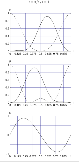
Figure 1: Model probabilities for vacuum neutrino oscillations as a function of the dimensionless distance $l$. The probabilities $P$ are calculated from Eqs. (17a)–(17i), with phase $\epsilon=\pi/4$ and energy-splitting ratio $r=1$. The top panel shows $P(C\rightarrow C)$ [broken curve] and $P(C\rightarrow A)$ [solid curve], with $P(C\rightarrow B)$ given by $1-P(C\rightarrow C)-P(C\rightarrow A)$. The middle panel shows $P(A\rightarrow A)$ [broken curve] and $P(A\rightarrow C)$ [solid curve], with $P(A\rightarrow B)=1-P(A\rightarrow A)-P(A\rightarrow C)$. The bottom panel gives the time-reversal asymmetry (23) for vacuum oscillations between $A$–type and $C$–type neutrinos. Based on the comparison with the K2K data for flavor identifications $|A\rangle=|\nu_{e}\rangle$ and $|C\rangle=|\nu_{\mu}\rangle$, the wavelength $l=1$ would correspond to approximately $1700\,\mathrm{km}$ (cf. Table 5.3).

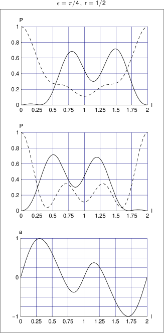
Figure 2: Same as Fig. 1 but for the energy-splitting ratio $r=1/2$. The wavelength $l=2$ would correspond to approximately $2400\,\mathrm{km}$, according to Table 5.3.

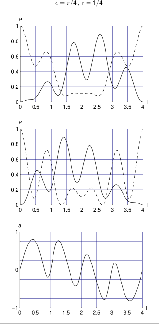
Figure 3: Same as Fig. 1 but for the energy-splitting ratio $r=1/4$. The wavelength $l=4$ would correspond to approximately $3800\,\mathrm{km}$, according to Table 5.3.

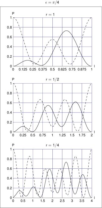
Figure 4: Model probabilities $P(B\rightarrow B)$ [broken curve] and $P(B\rightarrow C)$ [solid curve] as a function of the dimensionless distance $l$, with fixed phase $\epsilon=\pi/4$ and different energy-splitting ratios $r$. These probabilities are calculated from Eqs. (17a)–(17i) and $P(B\rightarrow A)$ is given by $1-P(B\rightarrow B)-P(B\rightarrow C)$. The flavor identifications from Eq. (29a) would be $|B\rangle=|\nu_{\tau}\rangle$ and $|C\rangle=|\nu_{\mu}\rangle$ and, according to Table 5.3, the wavelengths for $r=1,\,1/2$, and $1/4$ would correspond to some $1700$, $2400$, and $3800\,\mathrm{km}$, respectively.

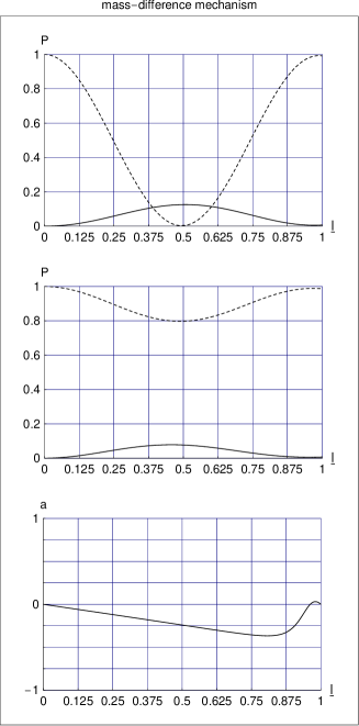
Figure 5: Probabilities $P$ for vacuum neutrino oscillations due to mass differences.[Bargeretal, McKeownVogel] The probabilities are calculated with the current best values $|\Delta m^{2}_{32}|=2\times 10^{-3}\;{\rm eV}^{2}/c^{4}$, $|\Delta m^{2}_{21}|=8\times 10^{-5}\;{\rm eV}^{2}/c^{4}$, $\sin^{2}(2\,\underline{\theta}_{\,32})=1$, $\sin^{2}(2\,\underline{\theta}_{\,21})=0.8$, and maximum allowed values $\sin^{2}(2\,\underline{\theta}_{\,13})=0.2$, $\underline{\delta}=\pi/2$. The top panel shows $P(\nu_{\mu}\rightarrow\nu_{\mu})$ [broken curve] and $P(\nu_{\mu}\rightarrow\nu_{e})$ [solid curve], as a function of the dimensionless distance $\underline{l}\equiv L\,|\Delta m^{2}_{32}|c^{4}/(2E_{\nu}hc)=(|\Delta m^{2}_{32}|\,c^{4})/(2\times 10^{-3}\;{\rm eV}^{2})\,(3\,\mathrm{GeV}/E_{\nu})\,L/(3720\,\mathrm{km})$. The middle panel shows $P(\nu_{e}\rightarrow\nu_{e})$ [broken curve] and $P(\nu_{e}\rightarrow\nu_{\mu})$ [solid curve]. The bottom panel gives the time-reversal asymmetry $a^{\mathrm{(T)}}$ for vacuum oscillations between $e$–type and $\mu$–type neutrinos, as defined by Eq. (23). Note that the distance $\underline{l}=1$ (corresponding to $L\approx 3720\,\mathrm{km}$, for neutrino energy $E_{\nu}=3\,\mathrm{GeV}$ and chosen parameters) is much less than the whole wavelength $\underline{l}=25$ ($L\approx 10^{5}\,\mathrm{km}$).

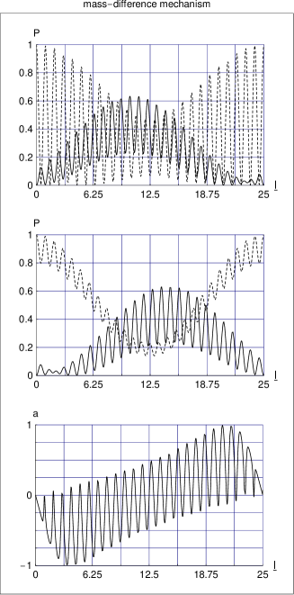
Figure 6: Same as Fig. 5 but now over the whole wavelength $\underline{l}=25$ (corresponding to $L\approx 9.3\times 10^{4}\,\mathrm{km}$, for neutrino energy $E_{\nu}=3\,\mathrm{GeV}$ and chosen parameters).

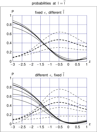
Figure 7: Model probabilities $P(\nu_{\mu}\rightarrow\nu_{\mu})$ [solid curves] and $P(\nu_{\mu}\rightarrow\nu_{e})$ [broken curves] as a function of parameter $z\equiv\log_{2}r$, evaluated at the dimensionless distance $\widehat{l}\equiv\tilde{l}\times 735/250$ and with flavor identifications (29). The curves of the top panel have phase $\epsilon=\pi/4$ and $\tilde{l}$ defined as the smallest distance for which $P(\nu_{\mu}\rightarrow\nu_{\mu})=0.70\pm 0.05$ [the central value $0.70$ corresponding to the heavy curves]. Specifically for the top panel, the broken curves at $z=1$ and the solid curves at $z=-3$, both from top to bottom, have $P(\nu_{\mu}\rightarrow\nu_{\mu})[\,\tilde{l}\,]=0.65,\,0.70,\,0.75$, respectively. The curves of the bottom panel have length $\tilde{l}$ defined as the smallest distance for which $P(\nu_{\mu}\rightarrow\nu_{\mu})=0.70$ and phase $\epsilon=5\pi/32,\,7\pi/32,\,\pi/4,\,9\pi/32,\,11\pi/32$ [the central value $\pi/4$ corresponding to the heavy curves]. Specifically for the bottom panel, the broken curves at $z=1$ from top to bottom have $\epsilon\times 32/\pi=5,\,7,\,8,\,9,\,11$, respectively, and the solid curves at $z=-3$ from top to bottom have $\epsilon\times 32/\pi=7,\,8,\,9,\,5,\,11$, respectively. The curves of this figure, with $\tilde{l}$ corresponding to the K2K baseline of $250\,\mathrm{km}$, may be relevant to the forthcoming MINOS experiment with a baseline of $735\,\mathrm{km}$. For comparison, the standard mass-difference model gives MINOS probabilities $P(\nu_{\mu}\rightarrow\nu_{\mu})\approx 66\,\%$ and $P(\nu_{\mu}\rightarrow\nu_{e})\lesssim 3\,\%$ for $E_{\nu}\approx 3\;\text{GeV}$ and $\sin^{2}(2\underline{\theta}_{13})\leq 0.2\,$; cf. Table 5.2.

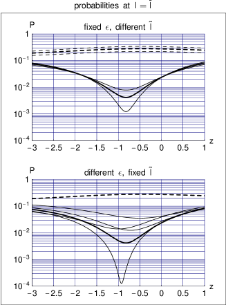
Figure 8: Model probabilities $P(\nu_{\mu}\rightarrow\nu_{e})$ [solid curves] and $P(\nu_{e}\rightarrow\nu_{\mu})$ [broken curves] as a function of parameter $z\equiv\log_{2}r$, evaluated at the dimensionless distance $\bar{l}\equiv\tilde{l}\times 295/250$ and with flavor identifications (29). The curves of the top panel have phase $\epsilon=\pi/4$ and $\tilde{l}$ defined as the smallest distance for which $P(\nu_{\mu}\rightarrow\nu_{\mu})=0.70\pm 0.05$ [the central value $0.70$ corresponding to the heavy curves]. Specifically for the top panel, the solid curves from top to bottom and the broken curves from bottom to top, both at $z=-1$, have $P(\nu_{\mu}\rightarrow\nu_{\mu})[\,\tilde{l}\,]=0.75,\,0.70,\,0.65$, respectively. The curves of the bottom panel have length $\tilde{l}$ defined as the smallest distance for which $P(\nu_{\mu}\rightarrow\nu_{\mu})=0.70$ and phase $\epsilon=5\pi/32,\,7\pi/32,\,\pi/4,\,9\pi/32,\,11\pi/32$ [the central value $\pi/4$ corresponding to the heavy curves]. Specifically for the bottom panel, the solid curves at $z=-0.5$ from top to bottom have $\epsilon\times 32/\pi=11,\,5,\,9,\,8,\,7$, respectively, whereas the broken curves have a rather narrow band on this logarithmic plot and only the heavy broken curve for $\epsilon=\pi/4$ is shown. The solid curves of this figure, with $\tilde{l}$ corresponding to the K2K baseline of $250\,\mathrm{km}$, may be relevant to the planned T2K (JPARC–SK) experiment with a baseline of $295\,\mathrm{km}$. For comparison, the standard mass-difference model gives a T2K probability $P(\nu_{\mu}\rightarrow\nu_{e})\lesssim 10\,\%$, according to Eq. (25a) for $\underline{\theta}_{32}=\pi/4$, $\sin^{2}(2\underline{\theta}_{13})\leq 0.2$, and $L$ near the first oscillation maximum.

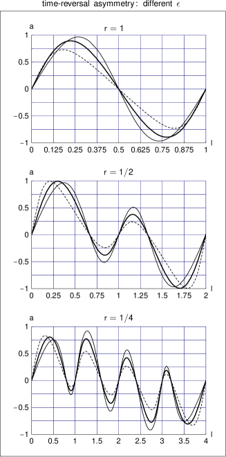
Figure 9: Model predictions for the time-reversal asymmetry (23) of vacuum oscillations between $e$–type and $\mu$–type neutrinos for different values of the energy-splitting ratio $r$ and different values of the phase, $\epsilon=5\pi/32,\,\pi/4,\,11\pi/32$ [the central value $\pi/4$ corresponding to the heavy curves, the low value to the broken curves, and the high value to the thin curves]. The probabilities entering the asymmetry parameter $a$ are calculated from Eqs. (17a)–(17i) and the flavor identifications are given by Eqs. (29). According to Table 5.3, the wavelengths for $r=1,\,1/2$, and $1/4$ would correspond to some $1700$, $2400$, and $3800\,\mathrm{km}$, respectively.

Figures 1–4 give the neutrino-oscillation probabilities for the phase $\epsilon=\pi/4$ but the same curves hold for $\epsilon=5\pi/4$ if the labels $B$ and $C$ are switched. Figure 4, for example, gives the $\epsilon=5\pi/4$ probabilities $P(C\rightarrow C)$ [broken curve] and $P(C\rightarrow B)$ [solid curve]. In the same way, Figs. 1–3 give the $\epsilon=5\pi/4$ probabilities $P(B\rightarrow B)$ and $P(B\rightarrow A)$ [top panels] and $P(A\rightarrow A)$ and $P(A\rightarrow B)$ [middle panels].

At this point, we can also mention that the model probabilities (17) for parameters (28)–(29) more or less fit the $L/E$ distribution from SK.[SuperK2004] A rough model estimate for atmospheric $\mu$–type events (normalized to the expected numbers without neutrino oscillations) shows, in fact, a significant “dip” down to some $45\,\%$ at $L/E$ values just under $10^{3}\;\mathrm{km}/\mathrm{GeV}$ and a “plateau” at the $58\,\%$ level for larger $L/E$ values, which more or less agrees with the experimental data (cf. Fig. 4 of Ref. SuperK2004). The same calculation gives for the normalized distribution of atmospheric $e$–type events an average value of $1$ with a dip at $L/E$ values of a few hundred $\mathrm{km}/\mathrm{GeV}$, which may perhaps be compared with Fig. 37 of Ref. KajitaTotsuka2001. Both dips can be understood heuristically from the relevant curves in Fig. 2, but a reliable model calculation requires further details on the energy spectra and experimental cuts. Recall that previous studies of atmospheric neutrino oscillations from alternative models[atmospheric] were performed in a two-flavor context.

We now turn to the predictions from the simple Fermi-point-splitting model (12)–(15) for future experiments. As benchmark results, we show in the last row of Table 5.2 probabilities for MINOS from standard mass-difference neutrinos oscillations (see also Figs. 5 and 6). Since K2K and MINOS in the low-energy mode have a similar $L/E$ ratio, the mass-difference mechanism for neutrino oscillations (25) predicts approximately equal probabilities. For the Fermi-point-splitting mechanism, only the travel distance $L$ enters and different probabilities may be expected in general. This is born out by the model values shown in the last column of Table 5.2.

According to Table 5.2, the allowed range of $r$ values from K2K and KamLAND is rather large, roughly between $1$ to $1/4$. MINOS, on the other hand, would allow for a more precise determination of $r$, assuming that the simple model has any validity at all. The top panel of Fig. 7 gives the model values for the $\epsilon=\pi/4$ probabilities $P(\nu_{\mu}\rightarrow\nu_{\mu})$ [solid curves] and $P(\nu_{\mu}\rightarrow\nu_{e})$ [broken curves] as a function of $r\equiv 2^{z}$. These probabilities are evaluated at a distance $\widehat{l}\equiv\tilde{l}\times 735/250$ corresponding to the MINOS baseline ($735\;\mathrm{km}$), provided $\tilde{l}$ corresponds to the K2K baseline ($250\;\mathrm{km}$) where $P(\nu_{\mu}\rightarrow\nu_{\mu})$ has been measured[K2K2002] to be approximately $0.70\pm 0.05$.

The simple model already makes the prediction that the appearance probability $P(\nu_{\mu}\rightarrow\nu_{e})$ from MINOS could be of the order of $10\,\%$ or more (see Fig. 7, top panel). This is substantially above the expectations from the standard mass-difference mechanism which predicts $P(\nu_{\mu}\rightarrow\nu_{e})$ of the order of a few percent at most (cf. Fig. 5), based on the stringent upper limits for $\underline{\theta}_{\,13}$ from CHOOZ[CHOOZ2002] and Palo Verde.[PaloVerde2001]

It is also clear from Fig. 7 [top panel] that a measurement of the survival probability $P(\nu_{\mu}\rightarrow\nu_{\mu})$ by MINOS would indeed allow for a better determination of the value of $r$ in the model, especially if combined with improved measurements of the same probability at $L=250-295\;\mathrm{km}$ from K2K[K2K2002, K2K2004] and T2K.[JPARCSK2001] In fact, the precise determination of $P(\nu_{\mu}\rightarrow\nu_{\mu})$ at $L=250\;\mathrm{km}$ would effectively collapse the bands in the top panel of Fig. 7. Assuming a measured value of $0.70$ for $P(\nu_{\mu}\rightarrow\nu_{\mu})$ at $L=250\;\mathrm{km}$, the variation with $\epsilon$ around a value of $\pi/4$ is shown in the bottom panel of Fig. 7. If MINOS would then measure $P(\nu_{\mu}\rightarrow\nu_{\mu})$ between $10\,\%$ and $60\,\%$, say, the further measurement of $P(\nu_{\mu}\rightarrow\nu_{e})$ could be used to constrain the value of $\epsilon$. The ICARUS[ICARUS] and OPERA[OPERA] experiments for the CNGS beam (with a similar baseline of $730\;\mathrm{km}$) may provide additional information through the measurement of the other appearance probability, $P(\nu_{\mu}\rightarrow\nu_{\tau})$, which could be $10\,\%$ or more according to our model (see the third entries of the last column of Table 5.2).

Even for the large mixing angle $\chi_{13}$ of the simple model (12)–(15), the probability $P(\nu_{\mu}\rightarrow\nu_{e})$ can be very low at $l\lesssim 0.25$, but the probability rapidly becomes substantial for larger values of $l$; see solid curves in top panels of Figs. 1–3. In contrast, mass-difference oscillations (25a) with a rather small $\underline{\theta}_{\,13}$ value[CHOOZ2002, PaloVerde2001] would have a reduced probability $P(\nu_{\mu}\rightarrow\nu_{e})$ over a larger range of dimensionless distance $\underline{l}\,$; compare top panels of Figs. 1 and 5. One of the main objectives of the planned T2K experiment (previously known as JPARC–SK) will be to measure this appearance probability at $L=295\;\mathrm{km}$. The relevant model values at $\bar{l}\equiv\tilde{l}\times 295/250$ are given in Fig. 8 [solid curves], together with the values for the time-reversed process [broken curves]. Typical values of $P(\nu_{\mu}\rightarrow\nu_{e})$ are seen to be around $1\,\%$, but lower values are certainly possible [for $\epsilon\approx 6.811\times\pi/32$, the lowest solid curve of the bottom panel drops to zero at $z\equiv\log_{2}r\approx-0.9426$].

Another quantity of practical importance to future experiments is the wavelength $\lambda$ (Table 5.3). In addition, there is the length $L_{\mathrm{magic}}$ where the time-reversal asymmetry (23) peaks, with $P(\nu_{\mu}\rightarrow\nu_{e})$ significantly less than $P(\nu_{e}\rightarrow\nu_{\mu})$. Table 5.3 gives the numerical values for this length and the corresponding asymmetry $a^{\mathrm{(T)}}_{\mu e}$. Remarkably, the value of $L_{\mathrm{magic}}$ is only weakly dependent on the model parameters $r$ and $\epsilon$; see Table 5.3 and Fig. 9. The other magic distance is $L^{\prime}\phantom{\!}_{\mathrm{magic}}\equiv\lambda-L_{\mathrm{magic}}$, with $P(\nu_{\mu}\rightarrow\nu_{e})$ significantly larger than $P(\nu_{e}\rightarrow\nu_{\mu})$. Table 5.3 shows that the $L^{\prime}\phantom{\!}_{\mathrm{magic}}$ value depends strongly on the model parameter $r$, because $\lambda$ does. For these large travel distances, matter effects need to be folded in, but the basic T–asymmetry $P(\nu_{e}\rightarrow\nu_{\mu})-P(\nu_{\mu}\rightarrow\nu_{e})$ is expected to be unaffected; cf. Refs. Bargeretal,McKeownVogel,Blondel2004.

With the identifications (29) and the large $\chi_{13}$ value (15) of the simple model, Table 5.3 shows that the distance $L_{\mathrm{magic}}$ would be at approximately $400\;\mathrm{km}$, which is not very much more than the T2K baseline of $295\;\mathrm{km}$.[JPARCSK2001] If the simple model of this article has any relevance, it would be interesting to have also initial $e$–type neutrinos for the T2K (JPARC–SK) baseline, possibly from a beta beam.[Zucchelli, Blondel2004]

Length scales for selected model parameters $B_{0}$, $r$, and $\epsilon$. With these parameters and identifications (29), the model (12)–(15) gives probability $P(\nu_{\mu}\rightarrow\nu_{\mu})\approx 0.70$ at $L=250\,\mathrm{km}$; cf. Table 5.2 and Eq. (27). An arbitrary distance $L$ is made dimensionless by defining $l\equiv B_{0}\,L/(h\,c)$, in terms of the basic energy-difference scale $B_{0}$. Shown are the (dimensionless) wavelength ($l_{\mathrm{wave}}$) $\lambda$, the (dimensionless) distance ($l_{\mathrm{magic}}$) $L_{\mathrm{magic}}$ which maximizes the time-reversal asymmetry $a^{\mathrm{(T)}}$ for $e$–type and $\mu$–type neutrinos as defined by Eq. (23), and the distance $L^{\prime}\phantom{\!}_{\mathrm{magic}}\equiv\lambda-L_{\mathrm{magic}}$ which minimizes the asymmetry (cf. bottom panels of Figs. 1–3). $B_{0}\,[10^{-12}\,\mathrm{eV}]\;$ $\;r\;$ $\;\;\epsilon\;$ $\;\;l_{\mathrm{wave}}\;$ $\;\lambda\;[\mathrm{km}]\;$ $\;\;\;l_{\mathrm{magic}}\;$ $\;L_{\mathrm{magic}}\;[\mathrm{km}]\;$ $\;a^{\mathrm{(T)}}_{\mu e}(L_{\mathrm{magic}})\;$ $\;\;L^{\prime}\phantom{\!}_{\mathrm{magic}}\;[\mathrm{km}]\;$ 0.72 1  $\;\;\;\pi/4\;\;$  1 1724    0.224  386  $+89\,\%$  1338 1.04 1/2  $\;\;\;\pi/4\;\;$  2 2381    0.300  357  $+99\,\%$  2024  1.29  1/4  $\;\;\;\pi/4\;\;$  4 3846    0.411  395  $+81\,\%$  3451