There is no local chiral perturbation theory at finite temperature

Abstract

For a low-temperature expansion in QCD it is well-known that the Lagrangian of vacuum chiral perturbation theory can be applied. This is due to the fact that the thermal effects of the heavy modes are Boltzmann suppressed. The present work is concerned with the situation of higher temperatures, but still below the chiral transition. For a systematic approach it would be desirable to have a temperature modified chiral perturbation theory at hand which would yield a chiral power counting scheme. It is shown that this cannot be obtained. In principle, chiral perturbation theory emerges from QCD by (a) integrating out all degrees of freedom besides the Goldstone bosons and (b) expanding the obtained non-local action in terms of derivatives. It is shown that at finite temperature step (b) cannot be carried out due to non-analyticities appearing for vanishing four-momenta. Therefore one cannot obtain a local Lagrangian for the Goldstone boson fields with temperature modified coupling constants. The importance of the non-analyticities is estimated.

I Introduction

Chiral perturbation theory ($\chi$PT) has become an important tool to describe in a systematic way low energy QCD (see e.g. Gasser and Leutwyler (1984, 1985); Ecker (1995); Pich (1995); Scherer (2003)). The spontaneous breakdown of chiral symmetry causes the appearance of (quasi-)Goldstone bosons which are much lighter than all other hadron species. In addition, chiral symmetry breaking enforces derivative couplings of the Goldstone bosons to themselves (and to all other hadrons) — besides terms which scale with the small mass of the Goldstone bosons. The gap in the excitations and the weakness of the couplings at small energies (and momenta) causes the success of $\chi$PT as a systematic approach to QCD (at low energies). To describe the interaction of the Goldstone bosons with themselves and with external sources (e.g. with photons) the effective Lagrangian of $\chi$PT is given by

$${\cal L}={1\over 4}\,F^{2}\,{\rm tr}\left(D_{\mu}UD^{\mu}U^{\dagger}+\chi U^{\dagger}+\chi^{\dagger}U\right)\quad\mbox{+ higher order terms.}$$ (1)

Corrections come with higher orders in powers of the involved energies and the Goldstone boson masses. Hence for sufficiently small energies these corrections are small and can be systematically taken into account up to the desired order. In (1) the Goldstone boson fields are encoded in the flavor matrix $U$. The masses of the Goldstone bosons as well as external scalar and pseudo-scalar fields are contained in $\chi$, derivatives as well as external vector and axial-vector fields in $D_{\mu}$ (cf. e.g. Gasser and Leutwyler (1984, 1985); Ecker (1995); Pich (1995); Scherer (2003) for details).

In principle, the coupling constants of $\chi$PT like $F$ given in (1) can be obtained from QCD by integrating out all degrees of freedom besides the Goldstone bosons. Such a task, however, would be more or less equivalent to solving QCD in the low-energy regime. Lattice QCD Creutz (1983) has started to determine some of these low-energy constants (see e.g. Giusti et al. (2004) and references therein). In practice, one determines these coupling constants from experiment Gasser and Leutwyler (1984, 1985); Amoros et al. (2001) or from hadronic Ecker et al. (1989a, b); Donoghue et al. (1989); Gomez Nicola and Pelaez (2002) or quark models Diakonov and Petrov (1986); Espriu et al. (1990); Schüren et al. (1992); Müller and Klevansky (1994); Pich (1995).

All the previous statements describe vacuum physics. In principle, it would be nice if the same worked at finite temperature $T$. For the following considerations we shall split the temperature region in three parts:

• Low temperatures: All thermal effects caused by the non-Goldstone modes are suppressed by Boltzmann factors $e^{-M_{h}/T}$ where $M_{h}$ is the mass of a non-Goldstone mode. At low temperatures one can neglect these effects. In this regime the Lagrangian (1) of vacuum $\chi$PT can be applied Goity and Leutwyler (1989); Gerber and Leutwyler (1989); Gerber et al. (1990); Schenk (1993). Of course, thermal propagators for the Goldstone bosons are used, but the input Lagrangian remains unaltered.

• Intermediate temperatures: In this regime the non-Goldstone modes become important. It ranges up to the chiral transition.

• High temperatures: Beyond the chiral and deconfinement transition quarks and gluons become the relevant degrees of freedom and form a quark-gluon plasma Hwa (1990, 1995).

QCD lattice calculations indicate that the temperature of the transition to the quark-gluon plasma is rather low (below 200 MeV Karsch (2002)) as compared to the typical hadronic scale of 1 GeV. Hence one might hope that the temperature regime II can still be described by a temperature-modified version of $\chi$PT. In the present work it is shown that this is NOT the case. In addition, we shall try to determine the temperature which splits regions I and II.

Formally $\chi$PT emerges from a two-step procedure. First, all other degrees of freedom besides the Goldstone bosons are integrated out. Suppose for the moment that this can be done — for the vacuum as well as for the finite temperature case. The result is a non-local action, schematically

$$S={\rm tr}\int\!\!d^{4}\!xd^{4}\!y\,D^{\mu}U(x)\,\Sigma_{\mu\nu}(x-y)\,D^{\nu}U^{\dagger}(y)+\ldots$$ (2)

In a second step the non-local kernels like $\Sigma_{\mu\nu}(x-y)$ have to be expanded to obtain a local action/Lagrangian. Technically this can be achieved e.g. by an expansion of the Fourier transform

$$\Sigma_{\mu\nu}(k)=\int\!\!d^{4}\!(x-y)\,\Sigma_{\mu\nu}(x-y)\,e^{ik(x-y)}$$ (3)

in powers of momenta $k$. This induces the first term within the trace in (1) and also higher order terms, since in coordinate space each $k$ translates to a derivative.

Let us first discuss why this two-step procedure works in vacuum. The conceptually crucial step is actually the second one. To expand (3) in powers of $k$ requires $\Sigma_{\mu\nu}(k)$ to be analytic. On the other hand, particle production thresholds cause cuts, i.e. non-analyticities. Fortunately all modes which are integrated out are rather heavy. Therefore the thresholds for their production are far away from $k=0$. Hence a rather broad energy range emerges where vacuum $\chi$PT can yield reliable results.

At finite temperatures the higher excited states (non-Goldstone modes) are already present in the heat bath. However, at low enough temperatures the corresponding Boltzmann factors suppress their influence to practically zero. Temperature regime I emerges.

Inspired by the success of vacuum $\chi$PT one might hope that temperature regime II can be similarly described by a modified version of $\chi$PT:

$${\cal L}(T)\stackrel{{\scriptstyle?}}{{=}}{1\over 4}\,{\rm tr}\left(F^{2}(T)\,D_{\mu}UD^{\mu}U^{\dagger}+\tilde{F}^{2}(T)\,D_{0}UD_{0}U^{\dagger}\right)\quad\mbox{+ mass and higher order terms}$$ (4)

with modified coupling constants, e.g.

$$F^{2}(T)=F^{2}+O\left(e^{-M_{h}/T}\right)$$ (5)

where $M_{h}$ denotes the mass of the lowest excited state besides the Goldstone modes and $F^{2}$ is the vacuum coupling constant from (1). The second term within the trace in (4) emerges due to the presence of a preferred rest frame (the heat bath):

$$\tilde{F}^{2}(T)=O\left(e^{-M_{h}/T}\right)\,.$$ (6)

In practice, it might be possible to obtain at least the lowest order coupling constants $F^{2}(T)$ and $\tilde{F}^{2}(T)$ from lattice QCD as suggested in Son and Stephanov (2002).

However, there are two problems with the considerations which have led to (4): First, in general, integrating out degrees of freedom causes imaginary parts for the kernels like $\Sigma_{\mu\nu}$ (see e.g. Greiner and Müller (1997); Greiner and Leupold (1998) and references therein). One can deal with that complication by a formal doubling of the degrees of freedom, e.g. by using the real time formalism Schwinger (1961); Bakshi and Mahanthappa (1963a, b); Keldysh (1964); Chou et al. (1985); Landsman and van Weert (1987); Das (1997). The second problem, however, is severe and the present work is devoted to that problem: If one integrates out specific heavy degrees of freedom at finite temperature, there appear kernels which are non-analytic at $k=0$. Such terms obviously invalidate any expansion in terms of local quantities. We should add here that non-analyticities are connected to thresholds and the latter are connected to imaginary parts of the kernels. Therefore the two mentioned problems are interrelated. Nonetheless we shall concentrate in the present work on the second problem, i.e. on non-analytic terms in the real parts of the kernels.

The fact that effective actions at finite temperatures might be manifestly non-local has been discussed e.g. in Weldon (1993); Arnold et al. (1993); Metikas (1999). The present work is an application of these findings to the case of $\chi$PT. For simplicity, we restrict ourselves to flavor-$SU(2)$. The pions are the lightest Goldstone bosons and therefore the most abandoned ones at finite temperature. The underlying physical mechanism for the non-analytic terms under consideration is the Landau damping process: (Virtual) Goldstone bosons scatter with a heavy mode from the heat bath and form another heavy state. If both heavy states have the same mass this damping process has its threshold at zero energy and momentum of the Goldstone boson. In the present work we will identify such processes and calculate the real parts of the pion self energies which correspond to the Landau damping mechanism.

A necessary condition for a local expansion of (2) is that the limit $k\to 0$ is well-defined for (3). Especially

$$\lim\limits_{\vphantom{\vec{k}}k_{0}\to 0}\,\lim\limits_{|\vec{k}|\to 0}\Sigma_{\mu\nu}(k)=\lim\limits_{|\vec{k}|\to 0}\,\lim\limits_{\vphantom{\vec{k}}k_{0}\to 0}\Sigma_{\mu\nu}(k)\,.$$ (7)

We will show in the present work by explicit examples that condition (7) is not satisfied for the strong interaction at finite temperature. Hence there is no local $\chi$PT for the finite temperature regime II. The big advantage of vacuum $\chi$PT as compared to standard phenomenological hadronic models is the existence of a systematic power counting scheme. Clearly a local theory is mandatory for such a scheme. The absence of local $\chi$PT at finite temperature means that a systematic power counting cannot be developed — at least not in the usual way. In other words, we are led back to conventional hadronic modeling for intermediate temperature low-energy QCD.

The rest of the paper is organized in the following way: In the next section we will present a non-analytic term appearing in the pion self energy by coupling the pion to $\rho$- and $\omega$-mesons. In Sec. III pions are coupled to constituent quarks. In Sec. IV we further discuss our results.

II Non-analytic term due to interaction with $\rho$- and $\omega$-mesons

It is the purpose of the present section to pin down the first sign of non-analyticity when increasing the temperature. Clearly, it has to be connected with the lowest massive excitations besides the Goldstone bosons. These are the vector mesons $\rho$ and $\omega$. In the following, we will neglect the very small mass difference between $\rho$- and $\omega$-meson and use $M_{V}\approx 770\,$MeV. We will come back to that point in the last section. Pions can be subject to Landau damping by scattering with one vector meson into the other one. An appropriate hadronic Lagrangian to describe such a process is given by Klingl et al. (1996)

$${\cal L}_{\rm int}={g_{VVP}\over 4f_{\pi}}\,\epsilon^{\mu\nu\alpha\beta}\,{\rm tr}\left(\partial_{\mu}V_{\nu}\,V_{\alpha}\,\partial_{\beta}\Phi\right)$$ (8)

with $g_{VVP}\approx 1.2$ and the pion decay constant $f_{\pi}\approx 92\,$MeV. $V$ describes the vector mesons and $\Phi$ the Goldstone bosons.

In the following we will calculate the thermal one-loop self energy of the $\pi^{0}$. In the loop we have the neutral $\rho$-meson $\rho^{0}_{\mu}$ and the $\omega$-meson $\omega_{\mu}$. The relevant parts of the quantities appearing in (8) are

$$\Phi\to\left(\begin{array}[]{cc}\pi^{0}&0\\ 0&-\pi^{0}\end{array}\right)\quad,\qquad V_{\mu}\to\left(\begin{array}[]{cc}\rho_{\mu}^{0}+\omega_{\mu}&0\\ 0&-\rho_{\mu}^{0}+\omega_{\mu}\end{array}\right)$$ (9)

and therefore

$${\cal L}_{\rm int}\to{g_{VVP}\over f_{\pi}}\,\epsilon^{\mu\nu\alpha\beta}\,\rho^{0}_{\mu}\,\partial_{\nu}\omega_{\alpha}\,\partial_{\beta}\pi^{0}\,.$$ (10)

The pion self energy is given by

$$\Pi_{h}(k)={g^{2}_{VVP}\over f_{\pi}^{2}}\,\epsilon^{\mu\nu\alpha\beta}\,\epsilon^{\mu^{\prime}\nu^{\prime}\alpha^{\prime}\beta^{\prime}}\,\int\!{d^{4}\!p\over(2\pi)^{4}}\,D^{\rho}_{\mu\mu^{\prime}}(p-k/2)\,D^{\omega}_{\alpha\alpha^{\prime}}(p+k/2)\,(p+k/2)_{\nu}\,(p+k/2)_{\nu^{\prime}}\,k_{\beta}\,k_{\beta^{\prime}}$$ (11)

with

$$D^{\rho/\omega}_{\mu\nu}(p)=\left(g_{\mu\nu}-{p_{\mu}p_{\nu}\over p^{2}}\right)\,D_{0}(p)+{p_{\mu}p_{\nu}\over p^{2}}\,{1\over M_{V}^{2}}$$ (12)

and the thermal free scalar boson propagator $D_{0}$ Das (1997). After some algebra one gets

$$\Pi_{h}(k)={g^{2}_{VVP}\over f_{\pi}^{2}}\,2\,k^{2}\int\!{d^{4}\!p\over(2\pi)^{4}}\,\left[\left(M_{V}^{2}+{k^{2}\over 4}\right)\,D_{0}(p-k/2)\,D_{0}(p+k/2)-{1\over 2}\,D_{0}(p)\right]\,.$$ (13)

As pointed out in the introduction we are interested in the behavior at small $k$. Here the leading non-analytic term is given by

$${\Pi_{h}^{\rm non-analyt}(k)\over k^{2}}={g^{2}_{VVP}\over f_{\pi}^{2}}\,2\,M_{V}^{2}\,I_{B}(k)$$ (14)

with

$$I_{B}(k)=\int\!{d^{4}\!p\over(2\pi)^{4}}\,D_{0}(p-k/2)\,D_{0}(p+k/2)-\left[\int\!{d^{4}\!p\over(2\pi)^{4}}\,D_{0}(p-k/2)\,D_{0}(p+k/2)\right]_{\rm vac}\,.$$ (15)

The small-$k$ behavior of this integral expression can be immediately taken over from Weldon (1993):

$$\left.\begin{array}[]{c}\lim\limits_{\vphantom{\vec{k}}k_{0}\to 0}\lim\limits_{|\vec{k}|\to 0}{\rm Re}I_{B}(k)\\[20.00003pt] \lim\limits_{|\vec{k}|\to 0}\lim\limits_{\vphantom{\vec{k}}k_{0}\to 0}{\rm Re}I_{B}(k)\end{array}\right\}={1\over 4\pi^{2}}\int\limits_{0}^{\infty}\!{dp\over\omega}\,n_{B}(\omega)\left\{\begin{array}[]{c}{\displaystyle p^{2}\over\displaystyle\omega^{2}}\\[15.00002pt] 1\end{array}\right.$$ (16)

with $\omega=\sqrt{p^{2}+M_{V}^{2}}$ and the Bose distribution

$$n_{B}(\omega)={1\over e^{\,\omega/T}-1}\,.$$ (17)

We take the difference between the two different limits given in (16) as a measure for the non-analyticity. We define

$$\Delta{\rm Re}I_{B}={1\over 4\pi^{2}}\int\limits_{0}^{\infty}\!{dp\over\omega}\,n_{B}(\omega)\left(1-{p^{2}\over\omega^{2}}\right)={M_{V}^{2}\over 4\pi^{2}}\int\limits_{0}^{\infty}\!{dp\over\omega^{3}}\,n_{B}(\omega)$$ (18)

and

$$\lim\limits_{k\to 0}{\Delta\Pi_{h}^{\rm non-analyt}(k)\over k^{2}}={g^{2}_{VVP}\over f_{\pi}^{2}}\,2\,M_{V}^{2}\,\Delta{\rm Re}I_{B}\,.$$ (19)

The expression (19) is shown in Fig. 1 as the full line. To get an idea about its size relative to other effects appearing at finite temperature we decided to show in Fig. 1 also the effect of the thermal wave function renormalization for the pion induced by thermal (massless) pion loops Pisarski and Tytgat (1996)

$$Z-1={T^{2}\over 12f_{\pi}^{2}}+o(T^{4})\,.$$ (20)

The expression (20) is depicted in Fig. 1 as the dashed line. We observe that even for temperatures as high as 200 MeV the non-analytic term due to the $\rho$-$\omega$ loop remains rather small.

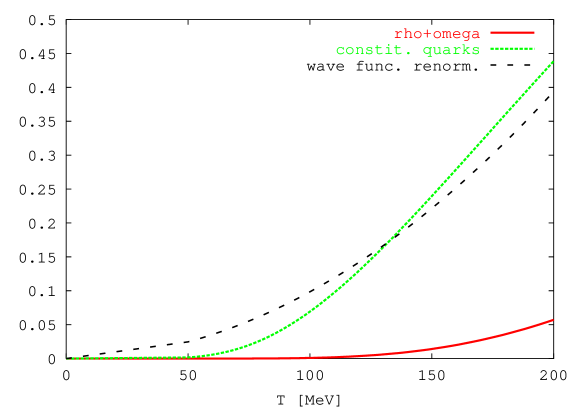
Figure 1: Non-analytic terms emerging from the interaction of pions with $\rho$- and $\omega$-mesons (full line) and constituent quarks (dotted line). For comparison the wave function renormalization $Z-1$ caused by thermal pions is also given (dashed line). See main text for details.

On the other hand, this is probably not the full story about non-analyticity. The vector mesons are the lightest non-Goldstone degrees of freedom. Therefore they show the first sign of non-analytic behavior. With rising temperature, however, also more massive modes become active. The pions might experience Landau damping by scattering on nucleons and other hadron species. (Note, however, that not all scattering events have their thresholds at vanishing $k$.) We try to effectively account for these processes in the next section.

III Non-analytic term due to constituent quarks

In the last section we have calculated a Landau damping contribution from scattering on vector mesons. The utilized Lagrangian (8) is phenomenologically rather well established. The content of the present section will be a little bit more speculative. Near the chiral transition more and more massive hadronic states become active and start to interact. One might reinterpret the rising scattering rates as a rising movability of the quarks contained in the hadrons. Therefore near the chiral transition it might be reasonable to describe the system effectively in terms of quarks instead of a large bunch of hadrons. Clearly below the transition these quarks have to be constituent quarks. We use the simplest possible model to describe the interaction of Goldstone bosons with quarks, the chiral constituent quark model with its Lagrangian Diakonov and Petrov (1986); Espriu et al. (1990); Christov et al. (1996)

$${\cal L}=\bar{q}\,\left(i\!\not\!\partial-MUP_{L}-MU^{\dagger}P_{R}\right)\,q$$ (21)

with the quark fields $q$, the Goldstone bosons encoded in

$$U=e^{-i\Phi/f_{\pi}}\,,$$ (22)

the projectors on right- and left-handed quarks

$$P_{R,L}={1\over 2}(1\pm\gamma_{5})$$ (23)

and the constituent quark mass $M$.

The self energy for the pion is given by

$$\Pi_{q}(k) = 2N_{c}\,{M\over f_{\pi}^{2}}\int\!{d^{4}\!p\over(2\pi)^{4}}\,{\rm tr}(\!\not\!p+M)\tilde{D}_{0}(p)+2N_{c}\,{M^{2}\over f_{\pi}^{2}}\int\!{d^{4}\!p\over(2\pi)^{4}}\,{\rm tr}[\gamma_{5}\,(\!\not\!p+M)\,\gamma_{5}\,(\!\not\!k+\!\not\!p+M)]\tilde{D}_{0}(p)\,\tilde{D}_{0}(k+p)$$ (24)

$$= 4N_{c}\,k^{2}\,{M^{2}\over f_{\pi}^{2}}\int\!{d^{4}\!p\over(2\pi)^{4}}\,\tilde{D}_{0}(p)\,\tilde{D}_{0}(k+p)$$

with the number of colors $N_{c}$ and the free fermion propagator Das (1997)

$$(\!\not\!p+M)\tilde{D}_{0}(p)\,.$$ (25)

We define in the way completely analogous to Sec. II:

$${\Pi_{q}^{\rm non-analyt}(k)\over k^{2}}=4N_{c}\,{M^{2}\over f_{\pi}^{2}}\,I_{F}(k)$$ (26)

with

$$I_{F}(k)=\int\!{d^{4}\!p\over(2\pi)^{4}}\,\tilde{D}_{0}(p)\,\tilde{D}_{0}(p+k)-\left[\int\!{d^{4}\!p\over(2\pi)^{4}}\,\tilde{D}_{0}(p)\,\tilde{D}_{0}(p+k)\right]_{\rm vac}\,,$$ (27)

$$\Delta{\rm Re}I_{F}={M^{2}\over 4\pi^{2}}\int\limits_{0}^{\infty}\!{dp\over\omega^{3}}\,n_{F}(\omega)$$ (28)

with the Fermi distribution

$$n_{F}(\omega)={1\over e^{\,\omega/T}+1}$$ (29)

and finally

$$\lim\limits_{k\to 0}{\Delta\Pi_{q}^{\rm non-analyt}(k)\over k^{2}}=4N_{c}\,{M^{2}\over f_{\pi}^{2}}\,\Delta{\rm Re}I_{F}\,.$$ (30)

This last expression is shown in Fig. 1 as the dotted line. For the numerics we have used a vacuum estimate for the constituent quark mass: $M\approx 350\,$MeV. In principle, one expects that $M$ drops near the chiral transition. In such a case the result would be even larger as the thermal suppression factor $e^{-M/T}$ (implicit in (28)) would be less effective. Therefore the dotted line in Fig. 1 provides a conservative estimate of the effect — provided one accepts on first place that the chiral constituent quark model yields a reasonable effective description of the system. Clearly one should not trust the results down to too low temperatures: There, thermal excitations have to scale with the Boltzmann factor of the lowest excitable mode, i.e. with $e^{-M_{V}/T}$ and not with $e^{-M/T}$ where again $M_{V}$ is the vector-meson mass and $M$ the constituent quark mass. At low temperatures the lack of confinement of (21) causes non-physical artifacts. Nonetheless, near the chiral transition the results might be more reasonable. With all these words of caution in mind we observe that there is a sizable non-analyticity induced by the Landau damping on constituent quarks for temperatures larger than $\approx 100\,$MeV.

IV Summary

The qualitative findings of the presented work and its consequences were already discussed in Sec. I and we do not repeat them here. Quantitatively, we have found that at least for the $\rho$-$\omega$ system the non-analyticities are rather small. Nonetheless, due to other heavy modes the effect might be important for temperatures between around 100 MeV and the chiral transition which is supposed to be somewhat below 200 MeV. We also want to stress that the discussed non-analyticities cannot be recovered in lattice QCD. Typical Minkowski-space features like Landau damping are absent in Euclidean-space calculations. This does not mean that the Euclidean calculations are wrong. It just tells that analytic continuation can be non-trivial Weldon (1993).

Coming back to the $\rho$-$\omega$ system there were two approximations which entered our calculation: First, strictly speaking the masses of $\rho$ and $\omega$ are not exactly the same. In principle, this allows for a local expansion around $k=0$. However, the range of applicability is limited to $k^{2}<M^{2}_{\omega}-M^{2}_{\rho}$ Arnold et al. (1993). There is no practical use for such an effective theory. Second, we have neglected the width of the vector mesons, especially the sizable one of the $\rho$-meson. It remains to be seen how the inclusion of the widths would influence the results. This is beyond the scope of the present work.

As already pointed out, the fact that there is no local $\chi$PT at finite temperature makes a systematic calculation of a given low-energy quantity much more complicated, if not impossible. Especially the interactions of heavier states with themselves are hard to incorporate systematically (in the vacuum this is all integrated out). What can be done for some quantities is the following: One might use the Lagrangian of vacuum $\chi$PT with thermal pions (cf. the description of temperature regime I above) and in addition a non-interacting gas of higher excited states. For the quark condensate this approach is utilized in Gerber and Leutwyler (1989). In practice, this might be sufficient up to temperatures rather close to the chiral transition. However, first, this approach is not fully systematic (i.e. it is not clear how to calculate corrections) and, second, it is not clear how to perform that for an arbitrary quantity (say, e.g. for the pion decay constant).

The Landau damping process, i.e. here the disappearance of a Goldstone boson by scattering on a heavy state into another heavy mode, can also be reinterpreted as a collective excitation. In that respect, it is the finite-temperature counterpart of a particle-hole excitation known from studies of cold nuclear matter Fetter and Walecka (1971). In other words, we have discussed the formation of a collective soft mode. In Son and Stephanov (2002) a local(!) in-medium pion Lagrangian was derived starting from hydrodynamic considerations. Collective soft modes as caused by Landau damping processes have not been considered there. It would be interesting to figure out how the considerations of Son and Stephanov (2002) would be influenced if such collective states were considered.