Abstract

A model is developed for electromagnetic form factor of the pion. One-loop corrections are included in the linear $\sigma-$model. The $\rho-$meson contribution is added in an extended VMD model. The form factor, calculated without fitting parameters, is in a good agreement with experiment for space-like and time-like photon momenta. Loop corrections to the two-pion hadronic contribution $a^{(had,\pi)}_{\mu}$ to the muon anomalous magnetic moment are calculated. The optimal value of the $\sigma-$meson mass appears to be close to the $\rho-$meson mass.

1 Introduction

It has recently been understood that the pion electromagnetic (EM) form factor is a very important physical quantity that plays a key role in the test of the Standard Model at the electroweak precision level. The reason is that the production cross section

$$\sigma(e^{+}e^{-}\rightarrow\pi^{+}\pi^{-})=\frac{\pi\alpha^{2}}{3s}\bigg{(}1-\frac{4m_{\pi}^{2}}{s}\bigg{)}^{3/2}|F_{\pi}(s)|^{2}\ ,$$ (1)

where $s$ is the squared total energy in center of mass system, $\alpha$ is the fine-structure constant and $m_{\pi}$ is the pion mass, at low energies dominates over the other hadronic channels and accounts for more than 70 per cent of the total hadronic contribution to the muon anomalous magnetic moment (AMM) $a_{\mu}=(g_{\mu}-2)/2$. The recent measurement of $a_{\mu}$ from Brookhaven E821 experiment [1] has boosted the interest in a renewed theoretical calculation of this quantity [2].

The main ingredient of the theoretical prediction of $a_{\mu}$, which is responsible for the bulk of the theoretical error, is the hadronic contribution to the vacuum polarization. The contribution of the $\pi^{+}\pi^{-}$ channel to the electron–positron annihilation process can be written in terms of the form factor $F_{\pi}(s)$ via the dispersion integral [3]

$$a^{(had,\pi)}_{\mu} = \frac{1}{4}\int_{4m^{2}_{\pi}}^{\infty}K(s)\bigg{(}1-\frac{4m_{\pi}^{2}}{s}\bigg{)}^{3/2}|F_{\pi}(s)|^{2}\ \mathrm{d}s,$$ (2)

$$K(s) = \frac{\alpha^{2}}{3\pi^{2}s}\int_{0}^{1}\frac{x^{2}(1-x)}{x^{2}+(1-x)s/m^{2}_{\mu}}\mathrm{d}x\ ,$$

where $m_{\mu}$ is the muon mass.

Conventional strategy of the model–independent evaluation of this integral consists in utilization of precise experimental data (at least at low energies, where perturbative $QCD$ cannot be reliably applied). However, the announced accuracy, which is to be reached soon in E821 experiment, requires calculation of EM radiative corrections to the cross section (1) [4]. Apart from the pure $\pi^{+}\pi^{-}$ events, EM radiative corrections include the $\pi^{+}\pi^{-}\gamma$ process, where photon is radiated from the final pions. In the current experiments at $\Phi$ and $B$ factories, based on radiative return method [5], this contribution cannot be extracted in a model–independent way and corresponding procedure requires model-dependent approaches. This, in turn, stimulates development and study of different theoretical models of pion-photon interaction. The simplest one is the point–like scalar quantum electrodynamics ($sQED$) [7] joined with standard Vector Meson Dominance (VMD) model (see, for example, [8]) for description of the $\gamma^{*}\rightarrow\pi^{+}\pi^{-}$ transition form factor in the $\rho$–resonance region. Such a model was used in Ref.[4] for construction of the Monte Carlo event generator.

In the present paper we consider modification of the pion EM form factor in the linear $\sigma-$model [9] with spontaneously broken chiral symmetry, which includes the nucleon sector. The $\rho-$meson contribution is added following Refs. [10, 11]. In particular, the $\rho$ coupling to the pion and nucleon is introduced through gauge-covariant derivatives, while direct $\gamma\rho$ coupling has explicitly gauge-invariant form. We calculate the pion form factor in one–loop approximation in the strong interaction and compare $F_{\pi}(s)$ with the precise data obtained from elastic $e^{-}\pi^{+}$ scattering and $e^{+}e^{-}$ annihilation in the pion pair.

We pay attention to the effect of the loop corrections in $a_{\mu}^{(had,\pi)}.$ In general, as Lagrangian of the $\sigma-$model contains Lagrangian of $sQED$ as a constituent part, one can expect that the difference between predictions of $\sigma-$model+VMD and $sQED$+VMD is small. Indeed, it follows from our calculation that the loop corrections increase the low-energy part of the right–hand–side of eq.(2) by about 2 per cent, as compared with $sQED$+VMD.

2
Formalism

2.1
Lagrangian

Lagrangian of the model consists of the two parts: ${\mathcal{L}}={\mathcal{L}}^{(1)}+{\mathcal{L}}^{(2)}$. The first one is Lagrangian of the chiral linear $\sigma-$model [9] with an explicit symmetry-breaking term $c\phi$. After spontaneous breaking of chiral symmetry and re-definition of the scalar field via $\phi=\sigma+v$, where $v=\langle\phi\rangle$ is vacuum expectation value, Lagrangian takes the form

$${\mathcal{L}}^{(1)} = \bar{N}(i\partial/-m_{N})N+\displaystyle{\frac{1}{2}\left[{(\partial\sigma)}^{2}-m_{\sigma}^{2}{\sigma}^{2}\right]}+\displaystyle{\frac{1}{2}\left[{(\partial{\vec{\pi}})}^{2}-m_{\pi}^{2}{\vec{\pi}\,}^{2}\right]}$$ (3)

$$-g_{\pi}\bar{N}\left(\sigma+i\gamma_{{}_{5}}\vec{\tau}\vec{\pi}\right)N-\lambda\left({\sigma}^{2}+{\vec{\pi}\,}^{2}\right)\left[v\sigma+\displaystyle{\frac{1}{4}\left({\sigma}^{2}+{\vec{\pi}\,}^{2}\right)}\right]+\mathrm{const},$$

where $N,\ \vec{\pi}\$ and $\sigma$ are the fields of the nucleon, pion and meson with vacuum quantum numbers, respectively, $g_{\pi}$ is the coupling constant, $\lambda$ is parameter of the meson potential, and $\partial/\equiv\partial^{\mu}\gamma_{\mu},$ $({\partial\sigma)}^{2}=\partial^{\mu}\sigma\partial_{\mu}\sigma,$ etc. All parameters of the model are related via

$$m_{N}=g_{\pi}v,\quad\quad\quad m_{\sigma}^{2}=2\lambda v^{2}+m_{\pi}^{2},\quad\quad\quad m_{\pi}^{2}=\frac{c}{v}.$$ (4)

Moreover, in the tree-level approximation $v=f_{\pi}$, where $f_{\pi}=93.2$ MeV is the pion weak-decay constant. More details on the $\sigma-$model can be found, for example, in [12], Ch.5, sect.2.6.

The second part of Lagrangian includes interaction with the EM field $A^{\mu},$ and the field $\rho^{\mu}$ of the neutral $\rho-$meson. This interaction can be obtained by using the minimal substitutions

$$\partial^{\mu}N \rightarrow (\partial^{\mu}+ie\frac{1+\tau_{3}}{2}A^{\mu}+ig_{\rho}\frac{\tau_{3}}{2}\rho^{\mu})N,$$

$$\partial^{\mu}\pi^{a} \rightarrow \partial^{\mu}\pi^{a}+(eA^{\mu}+g_{\rho}\rho^{\mu})\varepsilon^{3ab}\pi^{b},\,\ \ \ \ \ \ \ \ \ \ \ \ \ \ \ \ \ \ \ \ (a,b=1,2,3),$$ (5)

$$\partial^{\mu}\sigma \rightarrow \partial^{\mu}\sigma,$$

where $e$ is the proton charge, $g_{\rho}$ is the coupling constant, and $\tau_{3}$ is the third component of the Pauli vector $\vec{\tau}$ $=(\tau_{1},\tau_{2},\tau_{3}).$ In addition we include the direct coupling of the photon to the $\rho-$meson in the version of VMD model from Refs. [10, 11]. In this way we obtain

$${\mathcal{L}}^{(2)} = \displaystyle{\frac{1}{2}m_{\rho}^{2}\rho_{\mu}\rho^{\mu}-\frac{1}{4}\rho_{\mu\nu}\rho^{\mu\nu}-\frac{1}{4}F_{\mu\nu}F^{\mu\nu}}$$ (6)

$$-\left(eA_{\mu}+g_{\rho}\rho_{\mu}\right){\left(\vec{\pi}\times\partial^{\mu}\vec{\pi}\right)}_{3}+{\left(eA_{\mu}+g_{\rho}\rho_{\mu}\right)}^{2}({\vec{\pi}\,}^{2}-\pi_{{}_{3}}^{2})$$

$$-\displaystyle{g_{\rho}\bar{N}\gamma^{\mu}\frac{\tau_{{}_{3}}}{2}N\rho_{\mu}-e\bar{N}\gamma^{\mu}\frac{1+\tau_{{}_{3}}}{2}NA_{\mu}}\ {-\frac{e}{2f_{\rho}}\,\rho_{\mu\nu}F^{\mu\nu}}.$$

Here $F_{\mu\nu}=\partial_{\mu}A_{\nu}-\partial_{\nu}A_{\mu}$, $\rho_{\mu\nu}=\partial_{\mu}\rho_{\nu}-\partial_{\nu}\rho_{\mu}$ and $f_{\rho}$ determines the $\gamma\rho$ coupling. In eq.(6) we assumed equal coupling constants of the $\rho$ to the pion and the nucleon in accordance with the universality hypothesis of Sakurai (see, e.g., [12], Ch.5, sect.4). At the same time the $\gamma\rho$ coupling constant $f_{\rho}$ does not necessarily coincide with $g_{\rho}.$ Lagrangian (6) obeys gauge invariance because of the form of the $\gamma\rho$ coupling. We should mention that the nucleon contribution is also included in Lagrangian (6), contrary to [10, 11].

2.2 Counterterms and renormalization

Since one of the purposes of the present paper is to take into account loop corrections to the pion EM vertex one needs to specify the way of renormalization of the parameters. We use the conventional approach and assume that in Lagrangians (3) and (6) enter the “bare” fields, coupling constants and masses, to be marked by the subscript “0”. The bare fields require rescaling: $(\vec{\pi}_{0},\sigma_{0})=\sqrt{Z_{\pi}}(\vec{\pi},\sigma),\,N_{0}=\sqrt{Z_{N}}N,\,\rho_{0}^{\mu}=\sqrt{Z_{\rho}}\rho^{\mu}\,\$and$\ \ A_{0}^{\mu}=\sqrt{Z_{A}}A^{\mu},$ where $Z_{\pi,}Z_{N},Z_{\rho}$ and $Z_{A}$ are the respective wave-function renormalization constants for the pion (or sigma), nucleon, rho and photon. The procedure for obtaining Lagrangian of counterterms is known (see, for example, [13], Ch.10). For ${\mathcal{L}}^{(1)}$ the corresponding counterterm Lagrangian reads

$${\mathcal{L}}_{ct}^{(1)} = \delta_{Z_{N}}\bar{N}i\partial/N-\delta_{g_{\pi}}v\bar{N}N-\delta_{g_{\pi}}\bar{N}\left(\sigma+i\gamma_{{}_{5}}\vec{\tau}\vec{\pi}\right)N+\frac{1}{2}\delta_{Z_{\pi}}\left[{(\partial{\vec{\pi}})}^{2}+{(\partial\sigma)}^{2}\right]$$ (7)

$$-\frac{1}{2}\left(\delta_{\mu}+3\delta_{\lambda}v^{2}\right)\sigma^{2}-\frac{1}{2}\left(\delta_{\mu}+\delta_{\lambda}v^{2}\right){\vec{\pi}}^{2}-\frac{1}{4}\delta_{\lambda}{\left({\vec{\pi}}^{2}+\sigma^{2}\right)}^{2}-\delta_{\lambda}v\left(\sigma{\vec{\pi}}^{2}+\sigma^{3}\right)$$

$$-\left[\left(\delta_{\mu}+\delta_{\lambda}v^{2}\right)v-\delta_{c}\right]\sigma+\mathrm{const}.$$

There are six constants $\ \delta_{Z_{\pi}},\delta_{Z_{N}},\delta_{\mu},\delta_{\lambda},\delta_{g_{\pi}},\delta_{c},$ which can be fixed by imposing, in general, six conditions on the Green functions. In the calculation of the pion EM vertex only one constant $\delta_{Z_{\pi}}$ will be needed (see sect. 2.3).

For Lagrangian (6) one can define first the physical values of the electric charge $e=e_{0}\sqrt{Z_{A}}$ and the rho coupling $g_{\rho}=g_{\rho 0}\sqrt{Z_{\rho}}.$ It is also convenient to introduce $\hat{m}_{\rho}=\sqrt{Z_{\rho}}m_{\rho 0}$ ($\rho-$meson mass in the absence of the coupling to pions). The counterterm Lagrangian can be written as

$$\mathcal{L}_{ct}^{(2)} = -\delta_{Z_{A}}{\frac{1}{4}F_{\mu\nu}F^{\mu\nu}-}\delta_{Z_{\rho}}{\frac{1}{4}\rho_{\mu\nu}\rho^{\mu\nu}}$$ (8)

$$-\delta_{Z_{\pi}}\left(eA_{\mu}+g_{\rho}\rho_{\mu}\right){\left(\vec{\pi}\times\partial^{\mu}\vec{\pi}\right)}_{3}+\delta_{Z_{\pi}}{\left(eA_{\mu}+g_{\rho}\rho_{\mu}\right)}^{2}({\vec{\pi}\,}^{2}-\pi_{{}_{3}}^{2})$$

$$-\delta_{Z_{N}}{g_{\rho}\bar{N}\gamma^{\mu}\frac{\tau_{{}_{3}}}{2}N\rho_{\mu}-\delta_{Z_{N}}e\bar{N}\gamma^{\mu}\frac{1+\tau_{{}_{3}}}{2}NA_{\mu}}\ {-\delta}_{f_{\rho}}{\frac{e}{2}\,\rho_{\mu\nu}F^{\mu\nu}}.$$

It is seen, that in general one needs three additional constants $\delta_{Z_{A}},$ $\delta_{Z_{\rho}}$ and ${\delta}_{f_{\rho}},$ once $\delta_{Z_{\pi}}$ and $\delta_{Z_{N}}$ are fixed. Finally, the total Lagrangian is the sum

$$\mathcal{L}=\mathcal{L}^{(1)}+\mathcal{L}^{(2)}+\mathcal{L}_{ct}^{(1)}+\mathcal{L}_{ct}^{(2)}.$$ (9)

2.3 Contribution to pion EM form factor from the sector of $\sigma-$model

Feynman rules for Lagrangian (9) are obtained according to the standard prescriptions [14]. The counterterm constants can be found by imposing the following constraints on the self-energy operators of the pion, sigma-meson and nucleon respectively

$$\Sigma_{\pi}(m_{\pi}^{2}) = \frac{d}{dp^{2}}\Sigma_{\pi}(p^{2})\biggl{|}_{p^{2}=m_{\pi}^{2}}=\Sigma_{\sigma}(m_{\sigma}^{2})=0,$$ (10)

$$\Sigma_{N}(p/)\biggl{|}_{p/=m_{N}} = \frac{d}{dp/}\Sigma_{N}(p/)\biggl{|}_{p/=m_{N}}=0.$$

These conditions imply that the pole positions of the pion, nucleon and sigma propagators are located at the physical mass of the pion, nucleon and sigma respectively. In addition, the residue of the pion and nucleon propagators is unity, ensuring the absence of the renormalization for the external pion and nucleon (but not for the external sigma-meson). We also impose the condition $\langle\sigma\rangle=0$, which is ensured by requiring that the so-called tadpole diagrams vanish. Correspondingly, the tadpole diagrams will not contribute to quantities calculated below.

In calculation of the loop integrals we used the dimensional regularization method (see, e.g., [13], Appendix A.4). Exploiting the conditions (10) we find the constant $\delta_{Z_{\pi}}$:

$$\delta_{Z_{\pi}}=-\frac{g_{\pi}^{2}}{4\pi^{2}}\int_{0}^{1}\left[I_{\epsilon}-\ln\frac{\tilde{\Delta}_{N\pi}}{\Lambda^{2}}+\frac{m_{\pi}^{2}x(1-x)}{\tilde{\Delta}_{N\pi}}+\frac{{\left(m_{\sigma}^{2}-m_{\pi}^{2}\right)}^{2}x(1-x)}{4m_{N}^{2}\tilde{\Delta}_{\pi\sigma}}\right]\mathrm{d}x,$$ (11)

$$\tilde{\Delta}_{N\pi}=m_{N}^{2}-m_{\pi}^{2}x(1-x),\quad\ \ \tilde{\Delta}_{\pi\sigma}=m_{\sigma}^{2}x+m_{\pi}^{2}(1-x)^{2}.$$ (12)

In these equations $I_{\epsilon}=\displaystyle{\frac{2}{\epsilon}-\gamma_{E}+\ln 4\pi},\ \ \epsilon=4-D\rightarrow 0,\$ where $D$ is the space-time dimension, $\gamma_{E}\approx 0.5772$ is the Euler constant and $\Lambda$ is an arbitrary scale mass, which drops out in the physical observables.

The one-loop contributions to the pion EM vertex coming from the $\sigma-$model are shown in Fig. 1. Using the isospin structure of the vertices, or negative charge-conjugation parity of the photon, one can show that the diagrams “e,f” and “g” vanish. The counterterm “h” cancels divergences coming from the loop contributions “b” and “c”, while the contribution “d” is finite.

In general case of the off-mass-shell pions, the EM vertex $\Gamma_{ab}^{\mu}(p_{1},p_{2},q)$ for the process $\gamma^{\ast}(q)\rightarrow\pi^{a}(p_{1})+\pi^{b}(p_{2})$ has the form

$$-i\Gamma_{ab}^{\mu}(p_{1},p_{2},q)=\varepsilon^{3ab}\left[F(p_{1}^{2},p_{2}^{2},q^{2}){(p_{2}-p_{1})}^{\mu}+G(p_{1}^{2},p_{2}^{2},q^{2}){(p_{2}+p_{1})}^{\mu}\right],$$ (13)

with scalar functions $F(p_{1}^{2},p_{2}^{2},q^{2})$ and $G(p_{1}^{2},p_{2}^{2},q^{2}).$ On the mass shell, $p_{1}^{2}=p_{2}^{2}=m_{\pi}^{2}$, the function $G(m_{\pi}^{2},m_{\pi}^{2},q^{2})$ drops out, while $F(m_{\pi}^{2},m_{\pi}^{2},q^{2})$ becomes equal to the pion form factor $F_{\pi}(q^{2}).$ Denoting the loop corrections by  $\Delta F^{(\sigma)}(q^{2})$ we find

$$F_{\pi}^{(\sigma)}(q^{2})=1+\Delta F^{(\sigma)}(q^{2})+\delta_{Z_{\pi}},$$ (14)

where the total correction is finite and equal to

$$\Delta F^{(\sigma)}(q^{2})+\delta_{Z_{\pi}} = \frac{g_{\pi}^{2}}{4\pi^{2}}\biggl{[}\int_{0}^{1}\ \Bigl{(}\ln\frac{m_{N}^{2}-m_{\pi}^{2}x(1-x)}{m_{N}^{2}-q^{2}x(1-x)}-x(1-x)\bigl{[}\frac{m_{\pi}^{2}}{\tilde{\Delta}_{N\pi}}+\frac{{(m_{\sigma}^{2}-m_{\pi}^{2})}^{2}}{4m_{N}^{2}\tilde{\Delta}_{\pi\sigma}}\bigr{]}\Bigr{)}\mathrm{d}x$$ (15)

$$+\int_{0}^{1}\int_{0}^{1}\Bigl{(}\frac{y^{2}m_{\pi}^{2}}{\Delta_{N\pi}(y,x)}+\frac{y(1-y){(m_{\sigma}^{2}-m_{\pi}^{2})}^{2}}{4m_{N}^{2}\Delta_{\pi\sigma}(y,x)}\Bigr{)}\mathrm{d}x\mathrm{d}y\biggr{]},$$

$$\begin{split}\Delta_{N\pi}(y,x)&=m_{N}^{2}-q^{2}y^{2}x(1-x)-m_{\pi}^{2}y(1-y),\\ \Delta_{\pi\sigma}(y,x)&=m_{\sigma}^{2}(1-y)-y^{2}(q^{2}x(1-x)-m_{\pi}^{2})\end{split}$$ (16)

and $\tilde{\Delta}_{N\pi},\tilde{\Delta}_{\pi\sigma}$ are defined in eq.(12).

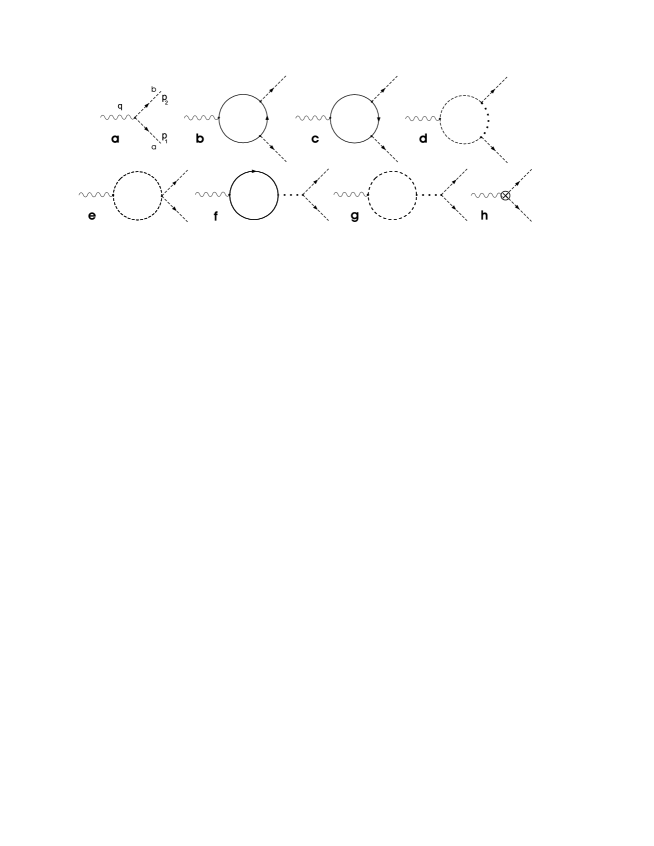
Figure 1: One-loop diagrams contributing to the pion EM form factor in the $\sigma-$model. Dashed lines depict pion, dotted lines – sigma, solid lines – nucleon, and wavy lines – photon. Small crossed circle denotes the counterterm. Diagram “a” corresponds to pion form factor in $sQED$.

2.4
Contribution to pion EM form factor from the $\rho-$meson

The contribution to the pion EM form factor from the $\rho-$meson can be written in the compact form

$$F_{\pi}^{(\rho)}(q^{2})=-\frac{g_{\rho}(q^{2})}{f_{\rho}(q^{2})}\frac{q^{2}}{q^{2}-\hat{m}_{\rho}^{2}-\Pi_{\rho}(q^{2})}+\Delta F_{\pi}^{(\rho\omega)}(q^{2}).$$ (17)

This expression includes several effects coming from the loop corrections which are shown in Fig. 2.

i) The $q^{2}-$dependent vertex $g_{\rho}(q^{2})$ describes loop corrections to the $\rho\pi\pi$ coupling, which originate from the $\sigma-$model (Fig. 2, diagrams “a”). These corrections have not been included in Ref.[11]. We can write

$$g_{\rho}(q^{2})=g_{\rho}[1+\Delta F^{(\sigma)}(q^{2})+\delta_{Z_{\pi}}].$$ (18)

It is seen that the expression in the square brackets is the same as in eq.(14) and is finite. From eq.(18) one obtains

$$g_{\rho}(q^{2})=g_{\rho}(m_{\rho}^{2})\frac{1+\Delta F^{(\sigma)}(q^{2})+\delta_{Z_{\pi}}}{1+\Delta F^{(\sigma)}(m_{\rho}^{2})+\delta_{Z_{\pi}}}$$ (19)

in terms of the constant $g_{\rho}(m_{\rho}^{2})$. From the experimental width of the $\rho\rightarrow\pi\pi$ decay,  $\Gamma_{\rho\rightarrow\pi\pi}$ = 150.7 MeV [15], we get $|g_{\rho}(m_{\rho}^{2})|=6.05.$ To find the real and imaginary part of $g_{\rho}(m_{\rho}^{2})$ one can make use of the relations

$$\mathrm{Re}\ g_{\rho}(m_{\rho}^{2})=\frac{1}{\sqrt{1+\lambda^{2}}}|g_{\rho}(m_{\rho}^{2})|,\quad\quad\quad\mathrm{Im}\ g_{\rho}(m_{\rho}^{2})=\frac{\lambda}{\sqrt{1+\lambda^{2}}}|g_{\rho}(m_{\rho}^{2})|,$$ (20)

$$\lambda={\mathrm{Im}\Delta F^{(\sigma)}(m_{\rho}^{2})}{[1+\mathrm{Re}\Delta F^{(\sigma)}(m_{\rho}^{2})+\delta_{Z_{\pi}}]^{-1}}.$$

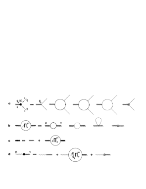
Figure 2: Diagrams “a” show $\pi,\sigma,N$ loop corrections to $\rho\pi\pi$ vertex; diagrams “b” – $\pi,N$ loop corrections to self-energy of $\rho-$meson; diagrams “c” graphically represent equation for exact $\rho-$meson propagator; diagrams “d” – $\pi,N$ loop corrections to $\gamma\rho$ vertex. Double-wavy lines depict $\rho-$meson. The corresponding counterterms are indicated by crossed circles.

ii) The $\rho-$meson self-energy has the structure $\ \Pi_{\rho}^{\mu\nu}(q)=(g^{\mu\nu}-q^{\mu}q^{\nu}/q^{2})\Pi_{\rho}(q^{2})$ and corresponds to the diagrams shown in Fig. 2 “b”.  It leads to the following exact propagator of the rho-meson (Fig. 2, diagrams “c”)

$$G_{\rho}^{\mu\nu}(q)=-i\frac{g^{\mu\nu}-q^{\mu}q^{\nu}/q^{2}}{q^{2}-\hat{m}_{\rho}^{2}-\Pi_{\rho}(q^{2})}+i\frac{q^{\mu}q^{\nu}}{q^{2}\hat{m}_{\rho}^{2}}.$$ (21)

Calculation of the loop integrals in Fig.2 “b” results in

$$\Pi_{\rho}(q^{2}) = q^{2}[\omega(q^{2})-\delta_{Z_{\rho}}],\,\ \ \ \ \ \ \ \ \ \ \ \ \ \omega(q^{2})=\frac{g_{\rho}^{2}}{16\pi^{2}}[-I_{\epsilon}+I(q^{2})],\,\ \$$ (22)

$$\ \ \ \ \ I(q^{2}) = 2\int_{0}^{1}[2x\ln\frac{\Delta_{N}}{\Lambda^{2}}+(1-2x)\ln\frac{\Delta_{\pi}}{\Lambda^{2}}](1-x)\mathrm{d}x,$$ (23)

with $\Delta_{N}=m_{N}^{2}-q^{2}x(1-x)$ and$\ \ \Delta_{\pi}=m_{\pi}^{2}-q^{2}x(1-x).$ The self-energy has the logarithmic divergence and needs renormalization. The authors of Ref.[11] renormalized the self-energy by applying a dispersion relation with two subtractions. We prefer an alternative method of counterterms which is expressed in eq.(22) through the constant $\delta_{Z_{\rho}}.$ One can fix the latter from the constraint on the self-energy at the physical mass $m_{\rho}$ of the $\rho-$meson:

$$\frac{d}{dq^{2}}\mathrm{Re}\ \Pi_{\rho}(q^{2})|_{q^{2}=m_{\rho}^{2}}=0\,\ \ \ \ \ \Rightarrow$$ (24)

$$\delta_{Z_{\rho}}=Z_{\rho}-1=\mathrm{Re}\ \omega(m_{\rho}^{2})+m_{\rho}^{2}\mathrm{Re}\ \omega^{\prime}(m_{\rho}^{2}),$$ (25)

where $\mathrm{Re}\ \omega^{\prime}(q^{2})\equiv\frac{d}{dq^{2}}\mathrm{Re}\ \omega(q^{2}).$ It is seen from eqs.(22) and (25) that the self-energy  $\Pi_{\rho}(q^{2})=q^{2}[\omega(q^{2})-\mathrm{Re}\ \omega(m_{\rho}^{2})-m_{\rho}^{2}\mathrm{Re}\ \omega^{\prime}(m_{\rho}^{2})]$ is finite. Near the physical mass the latter has the expansion

$$\mathrm{Re}\ \Pi_{\rho}(q^{2})=-m_{\rho}^{4}\mathrm{Re}\ \omega^{\prime}(m_{\rho}^{2})+{\cal O}((q^{2}-m_{\rho}^{2})^{2}),$$ (26)

and therefore the coupling $g_{\rho}$ is not renormalized due to the self-energy loops [11]. There is also a finite mass shift

$${m}_{\rho}^{2}-\hat{m}_{\rho}^{2}=-m_{\rho}^{4}\mathrm{Re}\ \omega^{\prime}(m_{\rho}^{2}).$$ (27)

For definition of $\hat{m}_{\rho}$ see the paragraph before eq.(8).

Above the two-pion threshold the self-energy acquires an imaginary part coming from the pion loop (the third diagram in Fig. 2 “b”). Namely, at $q^{2}<4m_{N}^{2}$ the imaginary part and the $q^{2}$-dependent $\rho\rightarrow\pi\pi$ decay width read respectively

$$\mathrm{Im}\ \Pi(q^{2}) = -\frac{g_{\rho}^{2}q^{2}}{48\pi}(1-\frac{4m_{\pi}^{2}}{q^{2}})^{3/2}\theta(q^{2}-4m_{\pi}^{2}),$$

$$\Gamma_{\rho}(q^{2}) = -\mathrm{Im}\ \Pi(q^{2})/\sqrt{q^{2}}.$$ (28)

iii) Closely related to the self-energy are the loop corrections to the $\gamma\rho$ coupling constant, shown in Fig. 2 “d”. The sum of all contributions is proportional to the tensor  $g^{\mu\nu}-q^{\mu}q^{\nu}/q^{2}$ similarly to the tree-level term. Introducing the $q^{2}$-dependent vertex one obtains

$$\frac{1}{f_{\rho}(q^{2})}=\frac{1}{f_{\rho}}-\frac{\omega(q^{2})}{g_{\rho}}+\delta_{f_{\rho}},$$ (29)

where $\delta_{f_{\rho}}$ can be fixed by requiring that on the mass shell, $q^{2}=m_{\rho}^{2}$, the coupling $f_{\rho}(m_{\rho}^{2})$ is related to the $\rho\rightarrow e^{+}e^{-}$ decay width. The experimental width $\Gamma_{\rho\rightarrow e^{+}e^{-}}=6.77$ KeV [15] is reproduced with $\ |f_{\rho}(m_{\rho}^{2})|\approx 5.03$.  From eq.(29) we find

$$\frac{1}{f_{\rho}(q^{2})}=\frac{1}{f_{\rho}(m_{\rho}^{2})}+\frac{1}{g_{\rho}}[\omega(m_{\rho}^{2})-\omega(q^{2})].$$ (30)

Here the real part of the constant $f_{\rho}(m_{\rho}^{2})$ is determined from $|f_{\rho}(m_{\rho}^{2})|$ and the imaginary part,  $\mathrm{Im}\ f_{\rho}(m_{\rho}^{2})$ $=|f_{\rho}(m_{\rho}^{2})|^{2}\mathrm{Im}\ \omega(m_{\rho}^{2})/g_{\rho}$. It is seen from (30) that the effective $\gamma\rho$ vertex is finite. A similar procedure for this vertex was used in [11], although only the real part of $\ f_{\rho}(m_{\rho}^{2})$ was taken from experiment.

Let us also mention that in calculation of $\Pi_{\rho}(q^{2})$ and $f_{\rho}(q^{2})$ we used $|g_{\rho}(m_{\rho}^{2})|$ (instead of $g_{\rho}$) in order to get the correct width of the $\rho-$meson.

iv) The last term in eq.(17) describes the $\rho-\omega$ interference due to the EM effects [8]. The explicit form of the contribution to the pion form factor can be taken from Ref.[16]:

$$\Delta F_{\pi}^{(\rho\omega)}(q^{2}) = -\varepsilon_{\rho\omega}\frac{g_{\rho}}{f_{\omega}}\frac{q^{2}}{q^{2}-m_{\omega}^{2}+im_{\omega}\Gamma_{\omega}},$$ (31)

$$\varepsilon_{\rho\omega} = \frac{\Pi_{\rho\omega}}{m_{\omega}^{2}-m_{\rho}^{2}-i[m_{\omega}\Gamma_{\omega}-m_{\rho}\Gamma_{\rho}(q^{2})]},$$ (32)

where $\Gamma_{\omega}=8.43$ MeV is the full decay width of the $\omega-$meson with mass $m_{\omega}$,  $f_{\omega}=17.05$ is the $\gamma\omega$ coupling constant which is fixed from the $\omega\rightarrow e^{+}e^{-}$ decay width $\Gamma_{\omega\to e^{+}e^{-}}=0.6$ KeV [15], and $\Pi_{\rho\omega}\approx-3.8\cdot 10^{-3}$ GeV² is the mixed $\rho-\omega$ self-energy.

3 Results and discussion

Let us first specify parameters of the model. The constant $g_{\pi}$ is determined from the tree-level Goldberger-Treiman relation $g_{\pi}=m_{N}/f_{\pi}$ (first equation in (4)), while $g_{\rho}(m_{\rho}^{2})$ and $f_{\rho}(m_{\rho}^{2})$ are fixed from experiment, as described in sec. 2.4. The $\sigma$ mass is chosen equal to the mass of the $\rho$, i.e. $m_{\sigma}=m_{\rho}$, in line with Ref.[17], where $\sigma$ and $\rho$ are assumed to be degenerate. Furthermore, $m_{\rho}=768.5$ MeV and $m_{\omega}=782.57$ MeV [15].

It is interesting to note that calculation of the self-energy of the $\rho-$meson gives $\hat{m}_{\rho}=795$ MeV. This value is rather close to the physical mass $m_{\rho}$. In this connection note that the authors of [11] fitted $\hat{m}_{\rho}$ from the $\pi\pi$ scattering and obtained 810 MeV. The difference in the above values of $\hat{m}_{\rho}$ is partially due to our taking into account the nucleon loop, which was not considered in [11].

As mentioned in sec. 2.4, both the real and imaginary parts of the coupling constants $g_{\rho}(m^{2}_{\rho})$ and $f_{\rho}(m^{2}_{\rho})$ have been included. The calculation yields: $\mathrm{Re}\ g_{\rho}(m_{\rho}^{2})=6.036,\ \mathrm{Im}\ g_{\rho}(m_{\rho}^{2})=0.405$, and $\mathrm{Re}\ f_{\rho}(m_{\rho}^{2})=4.96,\ \mathrm{Im}\ f_{\rho}(m_{\rho}^{2})=-0.82$. Taking into account the imaginary parts leads to a small correction to results obtained when setting $\mathrm{Im}\ g_{\rho}(m_{\rho}^{2})=\mathrm{Im}\ f_{\rho}(m_{\rho}^{2})=0$.

Our main results are demonstrated in Fig. 3 and Tables 1 and 2. The calculated pion form factor $|F_{\pi}(q^{2})|^{2}$ for space-like and time-like values of $q^{2}$ is presented in Fig. 3. Apparently the agreement with the data [18] from elastic electron-pion scattering, and the data [19] from $e^{-}e^{+}$ annihilation in two pions is quite good. We emphasize that in our approach there are no fitting or tuning parameters.

There is a strong interference of the two contributions, $F^{(\sigma)}_{\pi}$ and $F^{(\rho)}_{\pi}$, in the total form factor. We show in Fig. 3 separately contribution $F^{(\sigma)}_{\pi}$ (marked “$\sigma-$model”). It is seen from eqs.(17) and (18) that the $\rho$ contribution also includes $\pi,\sigma,N$ loops coming from the $\sigma-$model. Switching off these corrections, i.e. putting $\Delta F^{(\sigma)}(q^{2})+\delta_{Z_{\pi}}=0$, we obtain

$$F_{\pi}^{(sQED+VMD)}(q^{2})=1-\frac{g_{\rho}}{f_{\rho}(q^{2})}\frac{q^{2}}{q^{2}-\hat{m}_{\rho}^{2}-\Pi_{\rho}(q^{2})}+\Delta F_{\pi}^{(\rho\omega)}(q^{2}).$$ (33)

Here the first term corresponds to sQED, the second and the third terms are the $\rho-$meson contributions. Note, that eq.(33) corresponds to the extended version of VMD of Ref.[11]; in the “standard” VMD model [8] one has the dependence $\ m^{2}_{\rho}/[m^{2}_{\rho}-q^{2}-im_{\rho}\Gamma_{\rho}(q^{2})]$.

Our calculation shows that the difference between the form factor, calculated in $\sigma-$model+VMD (eqs.(14) and (17)), and that in $sQED$+VMD (eq.(33)) is small, and therefore the results for $sQED$+VMD are not plotted in Fig. 3. Nevertheless, the difference may show up in the integrated quantity $a^{(had,\pi)}_{\mu}$ for the muon AMM.

Figure 3: Pion EM form factor for space-like $q^{2}$ (left) and time-like $q^{2}$ (right). Experimental data are from [18] and [19] respectively.

$sQED$	$\sigma-$model	$sQED$	$\sigma-$model	$\sigma-$model	Ref.[2]
		+ VMD	+ VMD	+ VMD ($f_{\rho}=g_{\rho}$)
525	753	4667	4763	4745	4774 $\pm$ 51

Table 1: Two-pion contribution $a^{(had,\pi)}_{\mu}$ to the muon anomalous magnetic moment (in units $10^{-11}$). The upper integration limit in eq.(2) is 0.8 GeV².

$m_{\sigma}$, GeV	0.4	0.5	0.6	0.7	0.8	0.9	1.0	1.1	1.2
$a^{(had,\pi)}_{\mu}$, 10-11	4546	4583	4640	4710	4788	4867	4946	5024	5099

Table 2: Dependence of $a^{(had,\pi)}_{\mu}$ on the mass of $\sigma-$meson.

The calculated values of $a^{(had,\pi)}_{\mu}$ are shown in Table 1. In general, the loop corrections in the $\sigma-$model are important (compare the 1st and the 2nd columns). Their role is however diminished in the full calculation, which includes the dominant $\rho-$meson contribution (the 3rd and the 4th columns in Table 1). The difference between $\sigma-$model+VMD and $sQED$+VMD calculations is about 2%.

In this connection our result can be used to estimate the size of radiative corrections due to final-state-photon radiation in the $e^{+}e^{-}\to\pi^{+}\pi^{-}\gamma$ process. The corresponding contribution to the muon AMM, $a_{\mu}^{(had,\pi\gamma)}$, is calculated in [4] in framework of $sQED$+VMD. In general, $\sigma(e^{+}e^{-}\rightarrow\pi^{+}\pi^{-}\gamma)/\sigma(e^{+}e^{-}\rightarrow\pi^{+}\pi^{-})$ is of the order $\alpha$. We expect, that the model dependence of $a_{\mu}^{(had,\pi\gamma)}$ is similar to that of $a_{\mu}^{(had,\pi)}$. Therefore, the deviation of $a_{\mu}^{(had,\pi\gamma)}$ calculated in $sQED$+VMD, from $a_{\mu}^{(had,\pi\gamma)}$ in a more realistic model, for example, in $\sigma-$model+VMD, is about 2%. The overall model-dependence effect in the contribution $a_{\mu}^{(had,\pi\gamma)}$ to the muon AMM is of the order $\alpha\times 2\%\approx 0.015\%$ and is therefore negligible.

In the 5th column we show result obtained if we put $f_{\rho}=g_{\rho}$ in Lagrangian (6). This approximation corresponds to the full universality of Sakurai. In this case the renormalization procedure for the $\gamma\rho$ vertex changes and $\delta_{f_{\rho}}$ in eq.(8) is equal to $\delta_{Z_{\rho}}/g_{\rho}$. The numerical results for the form factor and $a^{(had,\pi)}_{\mu}$, however, change very little, e.g., for the integral by about 0.4%.

As mentioned above, in the calculation we chose the mass $m_{\sigma}=m_{\rho}$ for the $\sigma-$meson. This particle is associated with $f_{0}(400-1200)-$meson in [15]. In view of its undetermined status we study in Table 2 the dependence of the calculated integral $a^{(had,\pi)}_{\mu}$ on $m_{\sigma}$. As can be seen from Table 2, the integral varies considerably. Let us take the value 4774 $\pm$ 51 from [2] as a very accurate fit to the experimental integral. Then, for the indicated error bars we obtain the mass of the $\sigma$ in the interval from 720 to 850 MeV. The central value 785 MeV is surprisingly close to the $\rho-$meson mass. Therefore our calculation agrees with the hypothesis of Ref.[17] about degeneracy of $\sigma-$ and $\rho-$mesons.

In the calculations we took into account diagrams, where the $\rho-$meson enters only on the tree level. In particular, the loops with intermediate $\rho-$meson for the $\gamma\pi^{+}\pi^{-}$ and $\rho\pi^{+}\pi^{-}$ vertices are left out. Such contributions can be consistently considered in the models, in which $\rho-$meson is included together with its chiral partner, the axial-vector $a_{1}-$meson, for example, in the so-called gauged $\sigma-$model [20] or chiral quantum hadrodynamics [21, 22]. This work is planned for future.

4 Conclusions

We developed a model for EM vertex of the pion. The model is based on the linear $\sigma-$model, which generates the loops with intermediate pion, sigma and nucleon. The $\rho-$meson is included in line with an extended VMD model [11]. The coupling of the $\rho$ to the pion and nucleon is introduced through gauge-covariant derivatives, and the direct $\gamma\rho$ coupling has gauge-invariant form. The $\rho-$meson self-energy and modified $\gamma\rho$ vertex are generated by the pion and nucleon loops. The renormalization is consistently performed using the method of counterterms without cut-off parameters.

The pion EM form factor, calculated in one-loop approximation in the strong interaction, is in good agreement with the precise data obtained from elastic $e^{-}\pi^{+}$ scattering and $e^{+}e^{-}$ annihilation into $\pi^{+}\pi^{-}$. The effect of the $\sigma-$model loops turns out to be small.

We calculated the contribution of the $e^{+}e^{-}\rightarrow\pi^{+}\pi^{-}$ process to the muon AMM moment, $a^{(had,\pi)}_{\mu}$. The calculation agrees quite well (by 0.15%) with recent very accurate fit of Ref.[2]. The contribution of the $\sigma-$model loops to $a^{(had,\pi)}_{\mu}$ is about 2%.

We also estimated the size of the model-dependence effects in $a^{(had,\pi\gamma)}_{\mu}$, the contribution to the muon AMM from final-state-photon radiation in $e^{+}e^{-}\rightarrow\pi^{+}\pi^{-}\gamma$ process. It is about $\alpha\times 2\%\approx 0.015\%$ and is therefore negligible. Thus our calculation does not contradict to the conclusion of Ref.[4] that final-state radiative process $e^{+}e^{-}\rightarrow\pi^{+}\pi^{-}\gamma$ can be evaluated in scalar QED supplemented with VMD model.

The only free parameter of the model, which is not fixed from the experiment, is the $\sigma-$meson mass. Comparison with the fit of Ref.[2] strongly points to the value of this mass close to the mass of the $\rho-$meson. This conclusion is consistent with Ref.[17], where the mesons $\sigma$ and $\rho$ are assumed to be degenerate.

References

- [1] H.N. Brown et al., Phys. Rev. Lett. 86, 2227 (2001); G.W. Bennet et al., Phys. Rev. Lett. 89, 101804 (2002).
- [2] J.F. de Trocóniz and F.J. Ynduráin, Phys. Rev. D 65, 093001 (2002) [arXiv: hep-ph/0106025].
- [3] S.J. Brodsky and E. de Rafael, Phys. Rev. 168, 1620 (1968).
- [4] H. Czyz, A. Grezelinska, J.H. Kűhn and G. Rodrigo, arXiv: hep-ph/0308312, to be published in Eur. Phys. J.
- [5] A.B. Arbuzov, E.A. Kuraev, N.P. Merenkov and L. Trentadue, JHEP 12, 009 (1998) [arXiv: hep-ph/9804430]; S. Binner, J.H. Kűhn and K. Melnikov, Phys. Lett. B459, 279 (1999) [arXiv: hep-ph/9902399].
- [6] A. Hoefer, S. Jadach, J. Gluza and F. Jegerlehner, arXiv: hep-ph/0302258.
- [7] J. S. Shwinger. Particles, Sources, and Fields. Vol. 3, Redwood City, USA: Addison–Wesley (1989) p.99; M. Drees and K.I. Hikasa, Phys. Lett. B252, 127 (1990).
- [8] R.P. Feynman, Photon-Hadron Interactions, W.A. Benjamin, Inc. Reading, Massachusetts, 1972, Ch.VI.
- [9] M. Gell-Mann and M. Lévy, Nuovo Cimento 16, 705 (1960).
- [10] M. Herrmann, B.L. Friman and W. Nörenberg, Nucl. Phys. A560, 411 (1993).
- [11] E. Klingle, N. Kaizer and W. Weise, Z. Phys. A356, 193 (1996).
- [12] V. De Alfaro, S. Fubini, G. Furlan and S. Rossetti, Currents in Hadron Physics. North-Holland Publ. Company, Amsterdam-London, American Elsevier Publ. Company Inc., New York, 1973.
- [13] E.M. Peskin and D.V. Schroeder, An Introduction to Quantum Field Theory, Westview Press, 1995.
- [14] C. Itzykson and J.-B. Zuber, Quantum Field Theory, McGraw-Hill Book Company, 1980.
- [15] K. Hagiwara et al. (Particle Data Group), Phys. Rev. D 66, 010001 (2002) (URL: http://pdg.lbl.gov).
- [16] H.B. O’Connell, B.C. Pearce, A.W. Thomas and A.G. Williams, Phys. Lett. B354, 14 (1995).
- [17] S. Weinberg, Phys. Rev. Lett. 65, 1177 (1990).
- [18] S.R. Amendolia et al., Nucl. Phys. B277, 168 (1986).
- [19] L.M. Barkov et al., Nucl. Phys. B256, 365 (1985).
- [20] B.W. Lee and H.T. Nieh, Phys. Rev. 166, 1507 (1968).
- [21] B.D. Serot and J.D. Walecka, Acta Phys. Pol. B 21, 655 (1992).
- [22] A.Yu. Korchin, D. Van Neck and M. Waroquier, Phys. Rev. C 67, 015207 (2003) [arXiv: nucl-th/0302042].