Oscillations of neutrinos produced by a beam of electrons

Abstract

We analyze a thought neutrino oscillation experiment in which a beam of neutrinos is produced by electrons colliding with atomic nuclei of a target. The neutrinos are detected by observing charged leptons, which are produced by neutrinos colliding with nuclei of the detector. We consider the case when both the target and detector nuclei have finite masses. (The case of infinitely heavy nuclei was considered in the literature earlier.)

1 Introduction

Despite an impressive number of theoretical papers published during the last 40-50 years, the phenomenology and description of neutrino oscillations is still a subject of heated debates. In particular, there is no consensus on the assumptions of equal energies or equal momenta of the three neutrino mass eigenstates $\nu_{j}$, $j=1,2,3$.

The equal momenta scenario was introduced in a pioneering paper on neutrino oscillations by Gribov and Pontecorvo [1], used by Fritzsch and Minkowski [2] and then by many other authors. The equal energies scenario was presented by Kobzarev et al. [3], who considered all three virtual neutrinos produced by a monochromatic beam of electrons colliding with infinitely heavy nuclei ($M\to\infty$). Since the recoil energy of such nuclei is zero, all three neutrinos have equal energies, the same as the energy of the electron. Stodolsky [4], Lipkin [5] and Vysotsky [6] presented general arguments in favor of equal energy scenario for realistic thought experiments. Still, in the most recent and authoritative review of particle physics in the contribution by Kaiser [7] neutrinos oscillations are discussed on the basis of equal momentum scenario. Note that the same attitude one can find in his previous review [8], while in 2000 [9] both equal energy and equal momentum scenarios were considered on the same footing (all this - in the oversimplified ”neutrino plane wave approximation”).

In refs. [1],[2],[7],[8], [9] plane wave free neutrinos traveling from the production point $A$ to the detection point $B$ were considered without discussing their progenitors. We will refer to such descriptions as reduced ones. Following the argument of ref. [6] it is evident that in the ”reduced approach” only the equal energy scenario is self-consistent. Otherwise the neutrinos are produced at the point $A$ not in a given flavor state, but in a state whose flavor oscillates with time.

In ref. [3] the progenitor (electron) was described by a plane wave. There exists a vast literature in which both the progenitor and offspring particles are described not by plane waves but by wave packets (see review by Beuthe [10]). In the present paper our attention is concentrated on the incoming and outgoing particles. We will find that depending on the properties of these external particles both differences of energies and momenta of different neutrino mass eigenstates are non-vanishing, but the energy difference is much smaller than the momentum difference when the energy transfer to the target nucleus is small.

In this note we are going to consider a more realistic situation than in ref. [3], namely, when the beam of electrons is not monochromatic (it is described by a finite-size wave packet), and the mass of the target nucleus is finite. Now the recoil energy of the nucleus cannot be neglected. The detection of neutrino occurs when it interacts with another nucleus (in detector). When a nucleus is in a crystal it is described by a wave function with a characteristic momentum spread about 1 keV and vanishing mean momentum. When the nucleus is in gas, its momentum is not vanishing, while momentum spread is smaller. (Note that even for an infinitely heavy nucleus in crystal the spread of the momentum is non-zero).

We will prove that in the case of finite masses of nuclei $A$ or $B$ neutrino oscillations disappear in the limit of the vanishing momentum spread of the electron wave packet (plane wave limit).

The structure of this paper is the following. We introduce ”little donkey” diagram with a virtual neutrino propagating between production and detection points in section 2. The amplitude is derived and analyzed in section 3. The expression of the phase difference responsible for oscillations is discussed in section 4. The probability of neutrino oscillations and their suppression is discussed in section 5. Section 6 is devoted to concluding remarks.

2 Probability and ”little donkey” diagram

Let us consider interaction of an electron $e$ with a nucleus $A$ of mass $M_{A}$ in a target. Neutrino produced in this interaction collides later on in a detector with a nucleus $B$ of mass $M_{B}$ and produces a charged lepton $l$. As a result the whole process looks like $e+A+B\rightarrow l+C+D$, (see Fig. 1).

The electronic neutrino $\nu_{e}$ produced on nucleus $A$ is a superposition of three neutrino mass eigenstates: $\nu_{e}=\sum_{i}U_{ei}\nu_{i}$ where $\nu_{i}$ is the state with mass $m_{i}$. Each mass eigenstate propagates independently between nuclei $A$ and $B$. Interaction with $B$ results in projection of the three neutrino propagating states on the state $\nu_{l}=\sum_{i}U_{li}\nu_{i}$. Here $U$ is the unitary mixing matrix, the first and second indices of which denote respectively flavor and mass eigenstates.

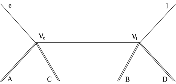
Figure 1: Little donkey diagram

In oscillation experiments the nuclei $C$ and $D$ are not registered, while the energy and momentum of the lepton $l$ are measured with low precision. Thus the probability of the whole process is obtained by integration of the amplitude squared, possibly weighted with the detector resolution function, over $d\mathbf{p}_{l}d\mathbf{p}_{C}d\mathbf{p}_{D}$

$$P(\mathbf{p}_{e},\mathbf{p}_{A,B},M_{A,B},\mathbf{x}_{A,B},\sigma_{A,B})=\int\sum_{i,j}U_{ei}U_{li}^{*}U_{ej}^{*}U_{lj}\times\\ \times P_{ij}(\mathbf{p}_{e,l},\mathbf{p}_{A,B},M_{A,B},\mathbf{x}_{A,B},\sigma_{A,B},\mathbf{p}_{C,D},E_{C,D})\frac{d\mathbf{p}_{l}}{2E_{l}}\frac{d\mathbf{p}_{C}}{2E_{C}}\frac{d\mathbf{p}_{D}}{2E_{D}}.$$ (1)

Here $P_{ij}=\mathcal{A}_{i}^{\star}\mathcal{A}_{j}$, where $\mathcal{A}_{i}$ is the amplitude for a given neutrino state with mass $m_{i}$; symbols like $\mathbf{p}_{A,B}$ denote $\mathbf{p}_{A}$, $\mathbf{p}_{B}$. Let us express $\mathcal{A}_{j}$ in terms of the wave functions of all interacting particles: $e,A,B,C,D,l$ and neutrino propagator $G(x_{1},x_{2})$ :

$$\mathcal{A}_{j}(\mathbf{p}_{e,l},\mathbf{p}_{A,B},M_{A,B},\mathbf{x}_{A,B},\sigma_{A,B},\mathbf{p}_{C,D},E_{C,D})=\int d\mathbf{x}_{1}d\mathbf{x}_{2}dt_{1}dt_{2}\times\\ \times\psi_{e}(\mathbf{x}_{1},t_{1})\psi_{A}(\mathbf{x}_{1},t_{1})\psi_{B}(\mathbf{x}_{2},t_{2})G_{j}(\mathbf{x}_{1},t,\mathbf{x}_{2},t_{2})\psi_{l}^{\ast}(\mathbf{x}_{2},t_{2})\psi_{C}^{\ast}(\mathbf{x}_{1},t_{1})\psi_{D}^{\ast}(\mathbf{x}_{2},t_{2}).$$ (2)

In ref. [3] electron $e$ and lepton $l$ were described by plane waves:

$$\begin{array}[]{rcl}\psi_{e}(\mathbf{x}_{1},t_{1})&=&e^{i\mathbf{p}_{e}\mathbf{x}_{1}-iE_{e}t_{1}},\\ \psi_{l}(\mathbf{x}_{2},t_{2})&=&e^{i\mathbf{p}_{l}\mathbf{x}_{2}-iE_{l}t_{2}},\\ \end{array}$$ (3)

while nuclei $A$ and $B$ were described by $\delta$-functions in configuration space .

Now we assume that nuclei $A$ and $B$ are described by the finite-size wave packets:

$$\begin{array}[]{rcl}\psi_{A}(\mathbf{x}_{1},t_{1})&=&\int e^{-\frac{(\mathbf{q}_{A}-\mathbf{p}_{A})^{2}}{2\sigma_{A}^{2}}}e^{i\mathbf{q}_{A}(\mathbf{x}_{1}-\mathbf{x}_{A})-iE_{A}(\mathbf{q}_{A})(t_{1}-t_{A})}d\mathbf{q}_{A}~{},\\ \psi_{B}(\mathbf{x}_{2},t_{2})&=&\int e^{-\frac{(\mathbf{q}_{B}-\mathbf{p}_{B})^{2}}{2\sigma_{B}^{2}}}e^{i\mathbf{q}_{B}(\mathbf{x}_{2}-\mathbf{x}_{B})-iE_{B}(\mathbf{q}_{B})(t_{2}-t_{B})}d\mathbf{q}_{B}~{},\end{array}$$ (4)

where $\mathbf{p}_{A}$ and $\mathbf{p}_{B}$ are the central momenta of the wave packets of nuclei $A$ and $B$ respectively, while $\mathbf{q}_{A}$ and $\mathbf{q}_{B}$ are the corresponding running momenta. In eqs. (4) and below we use Gaussian wave packets. The main features of our results do not depend upon the specific form of the packets. In our subsequent publication we are going to take for them a general form.

The wave functions of nuclei satisfy Klein-Gordon equation as we consistently neglect the spins of all particles. All external particles are assumed to be free and hence their momenta satisfy the on-mass-shell condition:

$$E_{n}(\mathbf{q}_{n})=\sqrt{\mathbf{q}_{n}^{2}+M_{n}^{2}}~{},$$ (5)

where the index $n$ denotes $A$, $B$ and $e$. The same is true also for outgoing particles.

Since in neutrino oscillation experiments the final nuclei $C$ and $D$ are not registered, one can choose for their wave functions any basis in the Hilbert space, and then integrate the probability over all Hilbert space. In what follows we take plane waves as the complete and orthogonal set of wave functions:

$$\begin{array}[]{rcl}\psi_{C}(\mathbf{x}_{1},t_{1})&=&e^{i\mathbf{p}_{C}\mathbf{x}_{1}-iE_{C}(t_{1}-t_{A})}~{},\\ \psi_{D}(\mathbf{x}_{2},t_{2})&=&e^{i\mathbf{p}_{D}\mathbf{x}_{2}-iE_{D}(t_{2}-t_{B})}~{},\end{array}$$ (6)

where $E_{C}^{2}=\mathbf{p}_{C}^{2}+M_{C}^{2}$ and $E_{D}^{2}=\mathbf{p}_{D}^{2}+M_{D}^{2}$. We think that description of outgoing particles by wave packets in the amplitude is not a consistent procedure, because generally wave packets do not have orthogonality property, neither they form a complete set of functions.

Here we would like to touch upon a subtle point. In a more or less realistic thought experiment the target and the detector are solids, therefore the on-mass-shell condition for nuclei is only an approximation. This approximation seems to be reasonable for ordinary matter, where nuclei are weakly bound.

Instead of the plane wave of ref. [3], the wave function of the electron is described now by the one dimensional wave packet with definite direction $\mathbf{e}={\mathbf{p}_{e}}/{|\mathbf{p}_{e}|}$ of the beam:

$$\psi_{e}(\mathbf{x}_{1},t_{1})=\int e^{-\frac{(\mathbf{q}_{e}-\mathbf{p}_{e})^{2}}{2\sigma_{e}^{2}}}e^{i\mathbf{q}_{e}\cdot(\mathbf{x}_{1}-\mathbf{x}_{e})-iE_{e}(\mathbf{q}_{e})(t_{1}-t_{e})}d\mathbf{q}_{e}.$$ (7)

Here and in the following:

$$d\mathbf{q}_{e}\equiv\delta(\mathbf{e}-\frac{\mathbf{q}_{e}}{|\mathbf{q}_{e}|})q_{e}^{2}dq_{e}d\Omega_{e},$$ (8)

where $\Omega_{e}$ is the corresponding solid angle, and $q_{e}\equiv|\mathbf{q}_{e}|$. We will show below that the oscillation terms vanish when $\sigma_{e}$ tends to zero. We choose the one-dimensional packet only because of technical simplicity. The result can be obtained in a more general case.

3 Neutrino Green function and the amplitude

Following ref. [3] we replace the neutrino Green function with the propagator of a scalar particle of mass $m_{j}$, where $j$ numerates neutrino mass eigenstates, $j=1,2,3$; it is clear that fermionic nature of the neutrino (as well as of $e$ and $l$) is not essential in the problem. Thus

$$G_{j}(\mathbf{x},t)=\frac{1}{(2\pi)^{4}}\int\frac{e^{-i\omega t+i\mathbf{k}\mathbf{x}}}{\omega^{2}-\mathbf{k}^{2}-m^{2}_{j}+i\varepsilon}d\mathbf{k}d\omega~{}.$$ (9)

For each $\nu_{j}$ the amplitude of the process is written as

$$\mathcal{A}_{j}=\int e^{-\frac{(\mathbf{p}_{e}-\mathbf{q}_{e})^{2}}{2\sigma_{e}^{2}}}e^{i\mathbf{q}_{e}(\mathbf{x}_{1}-\mathbf{x}_{e})-iE_{e}(t_{1}-t_{e})}d\mathbf{q}_{e}e^{-\frac{(\mathbf{q}_{A}-\mathbf{p}_{A})^{2}}{2\sigma_{A}^{2}}}e^{i\mathbf{q}_{A}(\mathbf{x}_{1}-\mathbf{x}_{A})-iE_{A}(\mathbf{q}_{A})(t_{1}-t_{A})}d\mathbf{q}_{A}\times\\ \times G_{j}(\mathbf{x}_{1}-\mathbf{x}_{2},t_{1}-t_{2})\times e^{-\frac{(\mathbf{q}_{B}-\mathbf{p}_{B})^{2}}{2\sigma_{B}^{2}}}e^{i\mathbf{q}_{B}(\mathbf{x}_{2}-\mathbf{x}_{B})-iE_{B}(\mathbf{q}_{B})(t_{2}-t_{B})}d\mathbf{q}_{B}e^{-i\mathbf{p}_{l}\mathbf{x}_{2}+iE_{l}(t_{2}-t_{B})}\\ \times e^{-i\mathbf{p}_{C}\mathbf{x}_{1}+iE_{C}(t_{1}-t_{A})}e^{-i\mathbf{p}_{D}\mathbf{x}_{2}+iE_{D}(t_{2}-t_{B})}d\mathbf{x}_{1}d\mathbf{x}_{2}dt_{1}dt_{2}=\\ =\int e^{-\frac{(\mathbf{p}_{e}-\mathbf{q}_{e})^{2}}{2\sigma_{e}^{2}}}e^{i\mathbf{q}_{e}(\mathbf{x}_{1}-\mathbf{x}_{e})+iE_{e}(t_{e}-t_{A})}e^{-\frac{(\mathbf{q}_{A}-\mathbf{p}_{A})^{2}}{2\sigma_{A}^{2}}}e^{i\mathbf{q}_{A}(\mathbf{x}_{1}-\mathbf{x}_{A})}e^{-\frac{(\mathbf{q}_{B}-\mathbf{p}_{B})^{2}}{2\sigma_{B}^{2}}}\times\\ \times e^{i\mathbf{q}_{B}(\mathbf{x}_{2}-\mathbf{x}_{B})}\frac{1}{4\pi|\mathbf{x}_{1}-\mathbf{x}_{2}|}e^{-ik_{j}|\mathbf{x}_{1}-\mathbf{x}_{2}|+i\omega\cdot(t_{A}-t_{B})}e^{-i\mathbf{p}_{l}\mathbf{x}_{2}}e^{-i\mathbf{p}_{C}\mathbf{x}_{1}-i\mathbf{p}_{D}\mathbf{x}_{2}}d\mathbf{x}_{1}d\mathbf{x}_{2}\times\\ \times\delta(E_{e}+E_{A}(\mathbf{q}_{A})+E_{B}(\mathbf{q}_{B})-E_{C}-E_{l}-E_{D})d\mathbf{q}_{e}d\mathbf{q}_{A}d\mathbf{q}_{B}~{},$$ (10)

where we use $dt_{1}dt_{2}=\frac{1}{2}d(t_{1}+t_{2})d(t_{1}-t_{2})$, and

$$\int e^{-i\omega(t_{1}-t_{2})}G_{j}(\mathbf{x}_{1}-\mathbf{x}_{2},t_{1}-t_{2})d(t_{1}-t_{2})=\frac{1}{4\pi|\mathbf{x}_{1}-\mathbf{x}_{2}|}e^{i\sqrt{\omega^{2}-m_{j}^{2}}|\mathbf{x}_{1}-\mathbf{x}_{2}|}~{}.$$ (11)

The parameter $\omega$ is defined by

$$\begin{array}[]{rcccccl}\omega&\equiv&\omega(\mathbf{q}_{A},\mathbf{q}_{B})&=&E_{e}+E_{A}(\mathbf{q}_{A})-E_{C}&=&E_{l}+E_{D}-E_{B}(\mathbf{q}_{B}),\end{array}$$ (12)

and

$$k_{j}\equiv\sqrt{\omega^{2}-m_{j}^{2}}.$$ (13)

Though $k_{j}$ looks like a three-momentum, in fact, it is a short-hand notation, usually arising in description of propagation of spherical waves with definite energy.

The integration over $d(t_{1}+t_{2})$ in eq.(10) gives $\delta$-function leading to energy conservation.

The further analysis of the problem is greatly simplified if the distance $|\mathbf{x}_{A}-\mathbf{x}_{B}|$ is much larger than the sizes of wave packets of nuclei $A$ and $B$. To take this into account, let us shift the variables of integration:

$$\left\{\begin{array}[]{rcl}\mathbf{x}_{1}&=&\mathbf{x}_{A}+\mathbf{x}_{1}^{\prime}\\ \mathbf{x}_{2}&=&\mathbf{x}_{B}+\mathbf{x}_{2}^{\prime}~{}~{}.\end{array}\right.$$ (14)

The wave packets of the nuclei $A$ and $B$ are essentially different from zero if $|\mathbf{x}_{1}^{\prime}|$, $|\mathbf{x}_{2}^{\prime}|\ll|\mathbf{x}_{A}-\mathbf{x}_{B}|$, hence

$$|\mathbf{x}_{1}-\mathbf{x}_{2}|\simeq|\mathbf{x}_{A}-\mathbf{x}_{B}|+(\mathbf{x}_{1}^{\prime}-\mathbf{x}_{2}^{\prime})\mathbf{n},$$ (15)

where $\mathbf{n}$ is the unit vector in the direction $\mathbf{x}_{A}-\mathbf{x}_{B}$.

By substituting eqs. (14) and (15) into eq. (10) we obtain after integration over $d\mathbf{x}_{1}^{\prime}$ and $d\mathbf{x}_{2}^{\prime}$:

$$\mathcal{A}_{j}\simeq\int\delta\left(\sum_{n=e,A,B}E_{n}(q_{n})-E_{C}-E_{l}-E_{D}\right)e^{i(\mathbf{q}_{e}-\mathbf{p}_{C})\mathbf{x}_{A}-i(\mathbf{p}_{l}+\mathbf{p}_{D})\mathbf{x}_{B}-i\mathbf{q}_{e}\mathbf{x}_{e}+iE_{e}(\mathbf{q}_{e})(t_{e}-t_{A})}\times\\ \times e^{-\sum_{n=e,A,B}\frac{(\mathbf{p}_{n}-\mathbf{q}_{n})^{2}}{2\sigma_{n}^{2}}}\delta(\mathbf{q}_{e}+\mathbf{q}_{A}-k_{j}\mathbf{n}-\mathbf{p}_{C})\delta(\mathbf{q}_{B}+k_{j}\mathbf{n}-\mathbf{p}_{l}-\mathbf{p}_{D})\times\\ \times\frac{\exp{\left\{ik_{j}|\mathbf{x}_{A}-\mathbf{x}_{B}|+i\omega_{j}(t_{A}-t_{B})\right\}}}{4\pi|\mathbf{x}_{A}-\mathbf{x}_{B}|}d\mathbf{q}_{e}d\mathbf{q}_{A}d\mathbf{q}_{B}=\\ =\int\delta(\sum_{n^{\prime}=A,B}E_{n^{\prime}}(q_{n^{\prime}j})+E_{e}(q_{e})-E_{C}-E_{l}-E_{D})\frac{e^{ik_{j}|\mathbf{x}_{A}-\mathbf{x}_{B}|+i\omega(\mathbf{q}_{Aj},\mathbf{q}_{Bj})\cdot(t_{A}-t_{B})}}{4\pi|\mathbf{x}_{A}-\mathbf{x}_{B}|}\times\\ \times e^{i(\mathbf{p}_{e}-\mathbf{p}_{C})\mathbf{x}_{A}-i(\mathbf{p}_{l}+\mathbf{p}_{D})\mathbf{x}_{B}-i\mathbf{p}_{e}\mathbf{x}_{e}+iE_{e}(t_{e}-t_{A})}e^{-\sum_{n^{\prime}=A,B}\frac{(\mathbf{p}_{n^{\prime}}-\mathbf{q}_{n^{\prime}j})^{2}}{2\sigma_{n^{\prime}}^{2}}-\frac{(\mathbf{p}_{e}-\mathbf{q}_{e})^{2}}{2\sigma_{e}^{2}}}d\mathbf{q}_{e}.$$ (16)

The $j$-dependent momenta $\mathbf{q}_{Aj}$ and $\mathbf{q}_{Bj}$ are defined as:

$$\begin{array}[]{rcl}\mathbf{q}_{Aj}&=&k_{j}\mathbf{n}+\mathbf{p}_{C}-q_{ej}\mathbf{e}~{},\\ \mathbf{q}_{Bj}&=&\mathbf{p}_{l}+\mathbf{p}_{D}-k_{j}\mathbf{n}~{}.\end{array}$$ (17)

We integrate over $d\mathbf{q}_{e}$ using (8). The result is:

$$\mathcal{A}_{j}\simeq|q_{ej}|^{2}\left(\frac{dE_{\Sigma}(q_{e})}{dq_{e}}\right)^{-1}\frac{e^{ik_{j}|\mathbf{x}_{A}-\mathbf{x}_{B}|+i\omega_{j}(t_{A}-t_{B})}}{4\pi|\mathbf{x}_{A}-\mathbf{x}_{B}|}\times\\ \times e^{i(q_{ej}\mathbf{e}-\mathbf{p}_{C})\mathbf{x}_{A}-i(\mathbf{p}_{l}+\mathbf{p}_{D})\mathbf{x}_{B}-i\mathbf{q}_{e}\mathbf{x}_{e}+iE_{e}(\mathbf{q}_{e})(t_{e}-t_{A})}e^{-\sum_{n=e,A,B}\frac{(\mathbf{p}_{n}-\mathbf{q}_{nj})^{2}}{2\sigma_{n}^{2}}},$$ (18)

where $\omega_{j}\equiv\omega(\mathbf{q}_{Aj},\mathbf{q}_{Bj})$ (see eq. (12)), $E_{\Sigma}(q_{e})\equiv\sum_{n^{\prime}=A,B}E_{n^{\prime}}(q_{n^{\prime}j})+E_{e}(q_{e})-E_{C}-E_{l}-E_{D}$, and $\left({dE_{\Sigma}(q_{e})}/{dq_{e}}\right)^{-1}$ is the Jacobian, left after integration of the energy $\delta$-function in (16). (In eq.(16) there are three $\delta$-functions, one of them expressing the energy conservation, while the other two refer to momentum conservation in $A$ and $B$ vertices.)

We have already stressed that $k_{j}$ is not a momentum, but a parameter characterizing spherical neutrino wave. Now we see that in the case of very large distance $|\mathbf{x}_{A}-\mathbf{x}_{B}|$ the parameter $k_{j}\mathbf{n}$ does play the role of the neutrino momentum. We are faced with the situation when neutrino being virtual particle at short distance from the source becomes effectively real at large distance, near detector.

4 Phases of the amplitudes

We are interested first of all in the phases of amplitudes of the process considered. From eq. (18) one can see that the phase of $\mathcal{A}_{j}$ equals to

$$\phi_{j}=k_{j}|\mathbf{x}_{A}-\mathbf{x}_{B}|+\omega_{j}(t_{A}-t_{B})+(q_{ej}\mathbf{e}-\mathbf{p}_{C})\mathbf{x}_{A}-\\ -(\mathbf{p}_{l}+\mathbf{p}_{D})\mathbf{x}_{B}-q_{ej}\mathbf{e}\mathbf{x}_{e}+E_{e}(p_{ej})(t_{e}-t_{A}),$$ (19)

and dependence of $k_{j}$, $q_{ej}$ and $\omega_{j}$ on $m_{j}$ is given by the system of equations (12), (13), (17), and by the on-mass-shell conditions for nuclei and electron.

From eq. (19) it follows that

$$\phi_{ij}\equiv\phi_{i}-\phi_{j}=|\mathbf{x}_{B}-\mathbf{x}_{A}|(k_{i}-k_{j})+(\omega_{i}-\omega_{j})(t_{A}-t_{B})+\\ +(q_{ei}-q_{ej})(\mathbf{x}_{A}-\mathbf{x}_{e})\mathbf{e}+(E_{e}(q_{ei})-E_{e}(q_{ej}))(t_{e}-t_{A}).$$ (20)

In equation (20) the difference of the electron energies could be expressed through the difference of the corresponding momenta:

$$(E_{e}(q_{ei})-E_{e}(q_{ej}))=\frac{dE_{e}(q_{e})}{dq_{e}}(q_{ei}-q_{ej}).$$ (21)

Since neutrino masses are much smaller than energies and momenta of external particles we may write:

$$\delta k_{ij}\equiv k_{i}-k_{j}\simeq(m^{2}_{i}-m^{2}_{j})\cdot\left.\frac{dk_{j}}{d(m_{j}^{2})}\right|_{m_{j}^{2}=0}=-\frac{m^{2}_{i}-m^{2}_{j}}{2\omega_{0}\cdot(1-\mathbf{v}_{B}\cdot\mathbf{n})},$$ (22)

$$\delta\omega_{ij}\equiv\omega_{i}-\omega_{j}\simeq(m^{2}_{i}-m^{2}_{j})\cdot\left.\frac{d\omega}{d(m_{j}^{2})}\right|_{m_{j}^{2}=0}=-\frac{(m^{2}_{i}-m^{2}_{j})}{2\omega_{0}}\cdot\frac{\mathbf{v}_{B}\cdot\mathbf{n}}{1-\mathbf{v}_{B}\cdot\mathbf{n}},$$ (23)

$$q_{ei}-q_{ej}\simeq(m^{2}_{i}-m^{2}_{j})\cdot\left.\frac{d\mathbf{q}_{ej}}{d(m_{j}^{2})}\right|_{m_{j}^{2}=0}=-\frac{(m^{2}_{i}-m^{2}_{j})}{2\omega_{0}\cdot(1-\mathbf{v}_{B}\mathbf{n})}\cdot\frac{(\mathbf{v}_{B}-\mathbf{v}_{A})\mathbf{n}}{(\mathbf{v}_{e}-\mathbf{v}_{A})\mathbf{n}},$$ (24)

where $\mathbf{v}_{n}\equiv{\mathbf{q}_{n0}}/{E_{n}(\mathbf{q}_{n0})}$, and the subscript $n$ denotes $e,~{}A,~{}B$.

The quantities $\mathbf{q}_{n0}$, $E_{n}(\mathbf{q}_{n0})$ and $\omega_{0}$ are defined by the external parameters from eqs. (12), (13), and (17) at $m_{j}=0$. In particular:

$$\omega_{0}=\frac{(\mathbf{p}_{D}-\mathbf{p}_{l})^{2}+M_{B}^{2}-(E_{D}+E_{l})^{2}}{2[(\mathbf{p}_{D}+\mathbf{p}_{l})\mathbf{n}-E_{D}-E_{l}]}\simeq\frac{(\mathbf{p}_{C}-\mathbf{p}_{e})^{2}+M_{A}^{2}-(E_{C}-E_{e}(\mathbf{p}_{e}))^{2}}{2[(\mathbf{p}_{e}-\mathbf{p}_{C})\mathbf{n}+E_{C}-E_{e}(\mathbf{p}_{e})]}.$$ (25)

In eq. (25) the sign ”=” means exact but somewhat useless equality, because $\mathbf{p}_{D}$ and $E_{D}$ are not measured, while $\mathbf{p}_{l}$ is measured with low accuracy. As for the sign ”$\simeq$”, it will be used in what follows because $\mathbf{p}_{e}$ and $E_{e}$ are known and essentially define the value of $\omega_{0}$:

$$\omega_{0}=E_{e}+O(\frac{1}{M_{A}})~{}.$$ (26)

From eqs. (20-24), it follows that

$$\phi_{ij}=\frac{m_{i}^{2}-m_{j}^{2}}{2\omega_{0}(1-\mathbf{v}_{B}\cdot\mathbf{n})}\times\\ \times\left(-|\mathbf{x}_{B}-\mathbf{x}_{A}|+(t_{B}-t_{A})\mathbf{v}_{B}\cdot\mathbf{n}+[(\mathbf{x}_{e}-\mathbf{x}_{A})\mathbf{e}-|\mathbf{v}_{e}|(t_{e}-t_{A})]\cdot\frac{(\mathbf{v}_{B}-\mathbf{v}_{A})\mathbf{n}}{(\mathbf{v}_{e}-\mathbf{v}_{A})\mathbf{n}}\right)~{}.$$ (27)

It is convenient to choose the parameters $t_{e}$, $t_{A}$, $\mathbf{x}_{e}$, and $\mathbf{x}_{A}$ in such a way that $\mathbf{x}_{e}=\mathbf{x}_{A}$ when $t_{e}=t_{A}$. This convention corresponds to the classical picture of $eA$-collision and allows to simplify eq. (27):

$$\phi_{ij}=\frac{m_{i}^{2}-m_{j}^{2}}{2\omega_{0}(1-\mathbf{v}_{B}\cdot\mathbf{n})}\left(-|\mathbf{x}_{B}-\mathbf{x}_{A}|+(t_{B}-t_{A})\mathbf{v}_{B}\cdot\mathbf{n}\right).$$ (28)

From eqs.(28), (22) and (23) it follows:

$$\phi_{ij}=\delta k_{ij}|{\bf x}_{B}-{\bf x}_{A}|-\delta\omega_{ij}(t_{B}-t_{A})=$$ (29)

$$=-\frac{m_{i}^{2}-m_{j}^{2}}{2\omega_{0}}|{\bf x}_{B}-{\bf x}_{A}|+\delta\omega_{ij}\left[|{\bf x}_{B}-{\bf x}_{A}|-(t_{B}-t_{A})\right].$$

The first term in the phase is the standard phase of oscillation theory, while the second one is an additional term which depends upon the size of the electron wave packet.

5 Neutrino oscillations and their suppression

By using eq. (10) we obtain the following expression for $P_{ij}$ describing neutrino oscillations in the right-hand side of eq. (1):

$$P_{ij}=e^{-i\phi_{ij}}\frac{|q_{ei}|^{2}|q_{ej}|^{2}}{16\pi^{2}|\mathbf{x}_{B}-\mathbf{x}_{A}|^{2}}\left(\frac{dE_{\Sigma}(q_{e})}{dq_{e}}\right)^{-2}\times\\ \times\exp\left(-\sum_{n=e,A,B}\frac{(\mathbf{p}_{n}-\mathbf{q}_{ni})^{2}}{2\sigma_{n}^{2}}-\sum_{n=e,A,B}\frac{(\mathbf{p}_{n}-\mathbf{q}_{nj})^{2}}{2\sigma_{n}^{2}}\right)~{},$$ (30)

where $\phi_{ij}$ is given by eq. (28).

This formula allows to compare the oscillating terms ($i\neq j$) with non-oscillating ($i=j$) ones, and thus to analyze the strength of oscillations as a function of the momentum spread of the electron wave packet.

For easier comparison with ref. [3] we assume in what follows that $\sigma_{e}$ is much smaller than $\sigma_{A}$ and $\sigma_{B}$. Let us define

$$f_{i}\equiv\exp(-\frac{(\mathbf{p}_{e}-\mathbf{q}_{ej})^{2}}{2\sigma_{e}^{2}})$$ (31)

and assume that $|\mathbf{p}_{e}-\mathbf{q}_{e1}|<|\mathbf{p}_{e}-\mathbf{q}_{e2}|,|\mathbf{p}_{e}-\mathbf{q}_{e3}|$, then $f_{1}\gg f_{2},f_{3}$ in the limit of vanishing $\sigma_{e}$. The leading diagonal term

$$P_{11}\sim f_{1}^{2}\gg P_{22},P_{33}.$$ (32)

Comparing $P_{11}$ with the non-diagonal terms we conclude:

$$P_{11}\sim f_{1}^{2}\gg P_{12}\sim f_{1}\cdot f_{2},~{}~{}~{}\mathrm{and}~{}~{}~{}P_{11}\gg P_{13},P_{23}.$$ (33)

Considering the ratio

$$\frac{f_{j}}{f_{i}}=\exp\left(-\frac{(\mathbf{p}_{e}-\frac{\mathbf{q}_{ej}+\mathbf{q}_{ei}}{2})}{\sigma_{e}^{2}}\cdot(\mathbf{q}_{ej}-\mathbf{q}_{ei})\right)$$ (34)

and using eq. (24) one finds the crucial parameter of suppression to be

$$\frac{q_{ej}-q_{ei}}{\sigma_{e}}=\frac{(\mathbf{v}_{B}-\mathbf{v}_{A})\cdot\mathbf{n}}{\sigma_{e}\cdot L_{ij}},$$ (35)

where

$$L_{ij}^{-1}\equiv\frac{(m^{2}_{i}-m^{2}_{j})}{2\omega_{0}}$$ (36)

is $ij$ oscillation length.

The Gaussian factor in eq.(30) makes it obvious that for $|\mathbf{q}_{ni}-\mathbf{q}_{nj}|\gg\sigma_{n}$, the oscillating terms become exponentially suppressed in comparison to the non-oscillating ones.

In conclusion of this section let us make the following remark. Though the suppression for vanishing $\sigma_{e}$ is obvious, it is clear, that in ”a realistic thought experiment” $\sigma_{e}^{-1}\ll L_{osc}$, and hence the suppression is very weak.

6 Concluding remarks

1) We see that the alternative ”equal energies versus equal momenta” is naturally resolved if one consistently uses the standard rules of quantum mechanics and in particular quantum field theory. In the example, which we consider here, using the propagator of virtual neutrinos and mixed description of initial (wave packets) and final (plane waves) particles all kinematical variables are uniquely defined. In particular, when we go beyond plane wave approximation for initial particles there is no equal momenta nor equal energies. However, still $|\omega_{j}-\omega_{i}|\ll|k_{j}-k_{i}|$ at least for non-relativistic nuclei. Similar conclusions were obtained in refs. [12], [13] for oscillating neutrinos produced in pion decay (see also [14]).
2) For the plane wave of the initial electron and finite mass nuclei, neutrino oscillations disappear unlike the case of infinitely heavy nuclei. For a finite but small momentum spread of the electron wave packet, the neutrino oscillations are suppressed.
3) For realistic parameters of the electron wave packet the above suppression is small and therefore can be disregarded.
4) The Green function used to describe neutrino leads us to the situation when the neutrino being a virtual particle at short distances from the source, becomes effectively a real particle at large distances, near detector. This is the standard case in the scattering theory.
5) With localized ”meeting points” $eA$ and $lB$ the time dependence of the oscillation probability is not essential. (The time moments $t_{A}$ and $t_{B}$ enter the expression for $\phi_{ij}$ with small coefficients proportional to velocities of nonrelativistic nuclei.)

7 Acknowledgments

We are grateful to M. Vysotsky for valuable comments. The work was partly supported by RFBR grants No. 2328.2003.2, No. 04-02 - 16538, by INTAS grant 00561 and by the A. von Humboldt award to L.O.

References

• [1] V.N. Gribov, B.M. Pontecorvo, Phys.Lett., 28 B (1969) 493.
• [2] H. Fritzsch, P. Minkowski, Phys. Lett. B 62 (1976) 72; Preprint CALT-68-525.
• [3] I.Yu. Kobzarev, B.V. Martemyanov, L.B. Okun and M.G. Schepkin, Sov. J. Nucl. Phys. 35 (1982) 708.
• [4] L. Stodolsky, Phys.Rev. D58 (1998) 036006.
• [5] H.J. Lipkin, hep-ph/9802387, hep-ph/0212093, v3, (2003).
• [6] M.I. Vysotsky, CKM matrix and CP violation in B-mesons. Surveys in High Energy Physics, 2003, vol. 18 (1-4), pp. 19-54; hep-ph/0307218, p.18.
• [7] B. Kaiser, Neutrino mass, mixing and flavor change, available on the PDG WWW pages (URL: http://pdg.lbl.gov/2004/reviews/), (2004)
• [8] B. Kaiser, Neutrino physics as explored by flavor change, Phys.Rev. D 66, (1 July 2002), p. 392.
• [9] B. Kaiser, Neutrino mass, Eur.Phys.Journal C 15, (2000), p. 344.
• [10] M. Beuthe, Phys.Rept. 375 (2003) 105-218, hep-ph/0109119/.
• [11] A.D. Dolgov, A.Yu. Morozov, L.B. Okun, M.G. Schepkin, Nucl.Phys., B 502 (1977) 3; hep-ph/9703241.
• [12] A.D. Dolgov, Neutrino Oscillations in Cosmology. A lecture presented at the 7th Course: Current Topics of Astrofundamental Physics ed. N. Sanchez, Erice-Sicile, 5-16 December, 1999 p. 565-584; hep-ph/0004032.
• [13] A.D. Dolgov, Phys. Rept. 370 (2002) 333.
• [14] M. Nauenberg, Phys. Lett. B 447 (1999) 23; Err.: Phys. Lett. B 452 (1999) 439; arXiv hep-ph/9812441.