Masses of Light Mesons
and Analytical Confinement

Abstract

Spectrum of masses of light pseudoscalar ($\pi,~{}K,~{}\eta,~{}\eta^{\prime}$) and vector ($\rho,~{}K^{*},~{}\omega,~{}\phi$) mesons can be explained on the base of the following assumptions: (1) analytical confinement (propagators of quarks and gluons are entire analytical functions of the Gaussian type), (2) mesons are bound states of quark and gluons (the Bethe-Salpeter equation in the one-gluon exchange approximation) and (3) QCD coupling constant $\alpha_{s}(M)$ is a monotone decreasing function of mass of a bound state $M$.

The decay constants $f_{\pi}$ and $f_{K}$ are calculated.

1 Introduction

At present time Quantum Chromodynamics (QCD) is considered as the true theory which control the behavior of quark and gluons as ”bricks” of hadron matter. Due to the confinement phenomena in experiments we observe colorless hadrons as bound states of quarks and gluons. Up to now a rigorous analytical solution of the problem of confinement and hadronization of quarks and gluons into hadrons is still missing. Therefore effective phenomenological and semi-phenomenological approaches based on QCD are developed to derive non-trivial statements about hadronic processes. Because dynamical mechanism of transformation of quarks and gluons into hadrons is not clear now the conception of quark and gluon structures depends on physical context under consideration and the aim of all theoretical approaches claiming to be obtained from ”the first principles” of QCD is to find process-independent concepts using symmetry and group arguments (chiral, flavour, anomaly, mixing and so on) in order to get possibilities to compare different characteristics of physical processes (there is huge literature on these problems, see, for example, [1, 2]).

We would like to stress that the application of methods of quantum field theory can be successful if (1) propagators of interacting particles are known and (2) the effective coupling constant is small. Namely this situation takes place in the standard model of electro-weak interactions. What have we in the QCD as theory of ”strong interactions”?

From physical point of view it is evident that processes of hadronization and confinement of quarks and gluons take place in the same space-time region, however the behavior of quarks and gluons in this confinement region is not known and, from our point of view, namely this circumstance is the main reason why QFT methods can not be applied directly. From our point of view if the behavior of quarks and gluons is known in the confinement region and the coupling constant is small enough, we will succeed in analytical solution of hadronization problem.

The idea to get the quark propagator in the confinement region is not new. The Schwinger-Dyson equation is the main tool to calculate this propagator (see, for example, [3, 4, 5]). However the theoretical problem is what quark-gluon vertex and what gluon propagator should be used in this equation and then what computing methods should be applied to get the solution of this equation. As a result calculations become to be very cumbersome and opaque (try to repeat these calculations!).

The confinement is generally accepted to be a result of nonperturbative nonlinear interactions of gluons in QCD. This idea plus the Wilson loop confinement argumentation are used to reduce the relativistic hadronization problem to a stationary Shrödinger picture with an increasing potential. Thus confinement is a static picture, i.e. there exists a constant in time potential which keep two quarks together. Conception of the confinement of one isolated quark is not formulated at all.

Our point of view (see [7]) is that the cause of confinement is instability of bosons in a homogeneous self-dual vacuum field. In particular in the quantum electrodynamics confinement can not take place because all fundamental particles (leptons and baryons) are fermions. In QCD gluons (bosons!) owing to nonlinear self-interaction play double role - they transfer the interaction as photons in QED and play role of real particles-bosons with zero mass. Namely massless gluons being bosons leads to instability of QCD-vacuum which is realized for a nonzero homogeneous self-dual vacuum gluon field which in turn leads to analytical confinement quark in this vacuum field. Thus from our point of view the initial ”free” quark-gluon Lagrangian should contain this field and propagators of quarks and gluons described by this ”free” Lagrangian should satisfy the confinement criterion. Physically analytical confinement means that quarks and gluons are fluctuations in space and time. Space-time scale of these fluctuations is defined by the strength of vacuum gluon field $\Lambda$.

The second question, what is the QCD coupling constant in the confinement region, i.e. for low energies $E\leq 1~{}Gev$? Usually coupling constant is supposed to be constant in this region although this statement is not completely consistent with general behavior of the running QCD coupling constant. Various investigations result in a remarkable variety of its infrared behavior (see [6]), so that this question can be considered to be open. Thus the unique answer this question is not yet exist, so that some speculations can be done.

The main subject of this paper is the spectrum of masses of light pseudoscalar ($\pi$, $K$, $\eta$, $\eta^{\prime}$) and vector ($\rho$, $K^{*}$, $\omega$, $\phi$) mesons. The aim of modern theoretical approaches is to get correlations between masses, i.e. so called mass formulas on the base of symmetry arguments (see, for example, [1]). Our point of view if the propagators of quarks and gluons are known in the confinement region and the QCD coupling constant $\alpha_{s}(M)$ is small enough, then the Bethe-Salpeter equation can be used to calculate desired masses.

The main result of this paper is that mass differences in pseudoscalar and vector multiples can be explained on the base of the following assumptions: (1) analytical confinement (propagators of quark and gluons are entire analytical functions of the Gaussian type), (2) mesons are bound states of quark and gluons (the Bethe-Salpeter equation in the one-gluon exchange approximation) and (3) QCD coupling constant $\alpha_{s}(M)$ is a monotone decreasing function of mass of a bound state $M$.

Our approach is based on the following statements

• The methods of Quantum Field Theory can be used, it means that weak coupling constant regime should take place and perturbation calculations can be applied.

• Our guess is that the selfdual homogeneous gluon fields with a constant strength is a good candidate to realize the vacuum QCD. In this fields analytical confinement takes place, i.e. propagators of quarks and gluons are entire analytical functions in the $p^{2}$ complex plane.

• If propagators of constituent particles are known and coupling constants are small enough bound states can be found as solutions of the Bethe-Salpeter equation in the one-gluon exchange approximation.

• The variation of the QCD coupling constant $\alpha_{s}(M)$ in the low energy region $M\leq 1~{}Gev$ should be taken into account.

Our aim is to understand the general features of spectrum of light mesons in the most simple dynamical way so that we want to simplify the problem as much as possible. The first observation is that the quark and gluon propagators can be approximated by virton fields, i.e. by pure Gaussian exponents. Besides solutions of the Bethe-Salpeter equation in this case can be found in the explicit analytical form, so that qualitative characteristics of the mass spectrum can be understood more profoundly (see [11]). The second observation is that for light quarks located in a selfdual homogeneous gluon fields with a constant strength the main contribution into quark propagators comes from so called zero modes. We show that these two points defines main features of light meson spectrum.

Thus our formulation of the problem looks:

Does it exist a reasonable form of propagators of quarks and gluons induced by the behavior of constituents in a selfdual homogeneous gluon fields with a constant strength and the QCD coupling constant $\alpha_{s}(M)$ in the region $M_{\pi}\leq M\leq M_{\eta^{\prime}}$ for which one can obtain the masses of pseudoscalar and vector mesons ?

2 Lagrangian and propagators.

Our basic assumption is that the QCD vacuum is realized by a self-dual gluon field with constant strength

$$\breve{B}_{\mu}(x)=B_{\mu}^{a}(x)t^{a},~{}~{}~{}~{}~{}B_{\mu}^{a}(x)=n^{a}B_{\mu}(x),~{}~{}~{}~{}~{}B_{\mu}(x)=\Lambda^{2}~{}b_{\mu\nu}x_{\nu},$$ (1)

$$B_{\mu\nu}(x)=\partial_{\mu}B_{\nu}(x)-\partial_{\nu}B_{\mu}(x)=-2\Lambda^{2}~{}b_{\mu\nu}={\rm const}.$$

Here $n^{a}$ is a constant vector in color space. The parameter $\Lambda$ defines the confinement scale and

$$b_{\mu\nu}=-b_{\nu\mu},~{}~{}~{}~{}b_{\mu\rho}b_{\rho\nu}=-\delta_{\mu\nu},~{}~{}~{}~{}\tilde{b}_{\mu\nu}={1\over 2}\epsilon_{\nu\mu\alpha\beta}b_{\alpha\beta}=\pm b_{\mu\nu}.$$

The field $\breve{B}_{\mu}(x)$ satisfies the Yang-Mills equations. The standard QCD Lagrangian in this field looks like

$${\cal L}=-{1\over 8}{\rm Tr}~{}{\breve{G}}_{\mu\nu}^{2}+\sum\limits_{f}\left(\bar{q}_{f}\left[\gamma_{\mu}(\breve{\nabla}_{\mu}+ig\breve{A}_{\mu})-m_{f}\right]q_{f}\right)$$ (2)

$${\breve{G}}_{\mu\nu}(x)=\breve{\nabla}_{\nu}{\breve{A}}_{\mu}-\breve{\nabla}_{\mu}{\breve{A}}_{\nu}+g[{\breve{A}}_{\mu}(x),{\breve{A}}_{\nu}(x)],~{}~{}~{}~{}~{}{\breve{A}}_{\mu}=t^{a}A_{\mu}^{a}$$

where

$$\breve{\nabla}_{\mu}(x)=\partial_{\mu}+i\breve{B}_{\mu}(x)=\partial_{\mu}+i\Lambda^{2}\breve{n}b_{\mu\nu}x_{\nu},$$

$$[\breve{\nabla}_{\mu}(x),\breve{\nabla}_{\nu}(x)]=-2i\Lambda^{2}\breve{n}b_{\mu\nu},~{}~{}~{}~{}~{}~{}\breve{n}=n^{a}t^{a}.$$

The part of the QCD Lagrangian which is responsible for meson hadronization can be written in the form

$${\cal L}=(\bar{q}S^{-1}q)-{1\over 2}(gD^{-1}g)+g(\bar{q}i\gamma_{\mu}t^{a}q)g_{\mu}^{a},$$ (3)

where the quark field $q(x)=q_{fa\alpha}(x)$ has indexes

$$f~{}-~{}{\rm flavor}~{}SU_{f}(3),~{}~{}a~{}-~{}{\rm color}~{}SU_{c}(3),~{}~{}\alpha~{}-~{}{\rm spin}$$

and the gluon field $g_{a\mu}(x)$ has

$$a~{}-~{}{\rm color}~{}SU_{c}(3),~{}~{}\mu~{}-~{}{\rm vector}.$$

The quark flavor spinor can be represented as

$$SU_{f}(3):~{}~{}~{}~{}~{}~{}~{}~{}q=\left(\begin{array}[]{c}u\\ d\\ s\\ \end{array}\right)$$

Quark propagator in the self-dual homogeneous gluon vacuum field is the solution of the equation (see details in [9])

$$(\hat{\nabla}(x)-m)S(x)=-\delta(x),~{}~{}~{}~{}~{}\nabla_{\mu}(x)=\partial_{\mu}+i\Lambda^{2}\breve{n}b_{\mu\nu}x_{\nu}.$$

It has the form

$$\tilde{S}_{\pm}(p) = \int\limits_{0}^{1}{du\over 2\Lambda^{2}}e^{-u{p^{2}\over 2\Lambda^{2}}}\left({1-u\over 1+u}\right)^{{m^{2}\over 4\Lambda^{2}}}$$

$$\cdot \left\{i\hat{p}\pm u\breve{n}\gamma_{5}(\gamma bp)+{m\over 1-u^{2}}\left[1\mp\gamma_{5}u^{2}+{i\over 2}\breve{n}(\gamma b\gamma)u\right]\right\}.$$

The gluon propagator is obtained in [10]. We do not show it here because formula is quite cumbersome.

We shall use the rough approximation of propagators preserving the main their features. The quark propagator having the Gaussian form and ”zero mode” behavior for small quark mass $\sim{1\over m}$ is chosen in the form

$$\tilde{S}_{f}(p) = \left({i\hat{p}\over\Lambda^{2}}+{1\pm\omega_{f}\gamma_{5}\over m_{f}}\right)e^{-{p^{2}\over 2\Lambda^{2}}}=\tilde{s}_{f}(p)e^{-{p^{2}\over 2\Lambda^{2}}},$$ (6)

$$\tilde{s}_{f}(p) = {i\hat{p}\over\Lambda^{2}}+{1\pm\omega_{f}\gamma_{5}\over m_{f}},~{}~{}~{}~{}~{}~{}\omega={1\over 1+{m^{2}_{f}\over\Lambda^{2}}}.$$

The gluon propagator is chosen in the form

$$D^{aa^{\prime}}_{\mu\mu^{\prime}}(x-x^{\prime})=\langle g_{a\mu}(x)g_{a^{\prime}\mu^{\prime}}(x^{\prime})\rangle=\delta^{aa^{\prime}}\delta_{\mu\mu^{\prime}}D(x-x^{\prime})$$

where

$$\tilde{D}(k)={1\over\Lambda^{2}}e^{-{k^{2}\over 2\Lambda^{2}}},~{}~{}~{}~{}~{}~{}D(y)={\Lambda^{2}\over(2\pi)^{2}}e^{-{\Lambda^{2}y^{2}\over 2}}$$ (7)

This rough choice of the quark and gluon propagators (6) and (7) is defined by the unique reason only: the Bethe-Salpeter equation can be solved analytically in this case and we get simple analytical formulas for the meson spectrum (see also [11]).

3 One-gluon exchange

In one-gluon exchange the four-quark interaction Lagrangian is

$$W = {g^{2}\over 2}\int\!\!\!\int dx_{1}dx_{2}(\bar{q}(x_{1})i\gamma_{\mu}t^{a}q(x_{1}))D(x_{1}-x_{2})(\bar{q}(x_{2})i\gamma_{\mu}t^{a}q(x_{2}))$$ (8)

In order to go to colorless quark currents the Fierz transformations should be done

• Color transformations

  $$SU_{c}(3):~{}~{}~{}~{}~{}~{}(t^{a})_{j_{1}j_{1}^{\prime}}(t^{a})_{j_{2}j_{2}^{\prime}}={4\over 9}\delta_{j_{1}j_{2}^{\prime}}\delta_{j_{2}j_{1}^{\prime}}-{1\over 3}(t^{a})_{j_{1}f_{2}^{\prime}}(t^{a})_{f_{2}f_{1}^{\prime}}$$

• Flavor transformations

  $$SU_{f}(3):~{}~{}~{}~{}~{}~{}\delta_{f_{1}f_{1}^{\prime}}\delta_{f_{2}f_{2}^{\prime}}={1\over 3}\delta_{f_{1}f_{2}^{\prime}}\delta_{f_{2}f_{1}^{\prime}}+{1\over 2}(\lambda^{a})_{f_{1}f_{2}^{\prime}}(\lambda^{a})_{f_{2}f_{1}^{\prime}}$$

• Dirac spin transformations

  $$(i\gamma_{\mu})_{\alpha_{1}\alpha_{1}^{\prime}}(i\gamma_{\mu})_{\alpha_{2}\alpha_{2}^{\prime}} = -{1\over 2}(i\gamma_{\mu})_{\alpha_{1}\alpha_{2}^{\prime}}(i\gamma_{\mu})_{\alpha_{2}\alpha_{1}^{\prime}}-(i\gamma_{5})_{\alpha_{1}\alpha_{2}^{\prime}}(i\gamma_{5})_{\alpha_{2}\alpha_{1}^{\prime}}$$

  $$- I_{\alpha_{1}\alpha_{2}^{\prime}}I_{\alpha_{2}\alpha_{1}^{\prime}}+{1\over 2}(\gamma_{\mu}\gamma_{5})_{\alpha_{1}\alpha_{2}^{\prime}}(\gamma_{\mu}\gamma_{5})_{\alpha_{2}\alpha_{1}^{\prime}}$$

Then for the four-quark interaction Lagrangian with pseudoscalar and vector colorless quark currents we get

$$W_{P} = {1\over 2}\cdot{4g^{2}\over 9}\int\!\!\!\int dx_{1}dx_{2}~{}D(x_{1}-x_{2})$$

$$\cdot \left\{{1\over 3}(\bar{q}(x_{1})i\gamma_{5}q(x_{2}))(\bar{q}(x_{2})i\gamma_{5}q(x_{1}))+{1\over 2}(\bar{q}(x_{1})i\gamma_{5}\lambda^{a}q(x_{2}))(\bar{q}(x_{2})i\gamma_{5}\lambda^{a}q(x_{1}))\right\},$$

$$W_{V} = {1\over 2}\cdot{2g^{2}\over 9}\int\!\!\!\int dx_{1}dx_{2}~{}D(x_{1}-x_{2})$$

$$\cdot \left\{{1\over 3}(\bar{q}(x_{1})i\gamma_{\mu}q(x_{2}))(\bar{q}(x_{2})i\gamma_{\mu}q(x_{1}))+{1\over 2}(\bar{q}(x_{1})i\gamma_{5}\lambda^{a}q(x_{2}))(\bar{q}(x_{2})i\gamma_{5}\lambda^{a}q(x_{1}))\right\}.$$

Flavor structure of meson currents looks like

$${1\over 3}(\bar{q}q)(\bar{q}q)+{1\over 2}(\bar{q}\lambda^{a}q)(\bar{q}\lambda^{a}q)$$

$$=\left[\cos\theta(\bar{n}n)+\sin\theta(\bar{s}s)\right]^{2}+\left[-\sin\theta(\bar{n}n)+\cos\theta(\bar{s}s)\right]^{2}$$

$$+(\bar{n}\tau^{j}n)(\bar{n}\tau^{j}n)+2[(\bar{u}s)(\bar{s}u)+(\bar{d}s)(\bar{s}d)]$$

where

$$n={1\over 2^{1/4}}\left(\begin{array}[]{c}u\\ d\\ \end{array}\right),~{}~{}~{}~{}~{}~{}(\bar{n}n)={(\bar{u}u)+(\bar{d}d)\over\sqrt{2}}$$

The ideal mixing angle is

$$\theta_{id}=\arcsin{1\over\sqrt{3}}=35.3^{\circ}$$

Pseudoscalar nonet is defined as

$$\pi^{j}=\bar{n}\tau^{j}n,~{}~{}~{}~{}~{}~{}K^{-}=\bar{u}s,$$ (11)

$$\eta=\cos\theta\cdot{\bar{u}u+\bar{d}d\over\sqrt{2}}+\sin\theta\cdot\bar{s}s,~{}~{}~{}~{}~{}~{}~{}\eta^{\prime}=-\sin\theta\cdot{\bar{u}u+\bar{d}d\over\sqrt{2}}+\cos\theta\cdot\bar{s}s.$$

Vector nonet is defined as

$$\rho^{j}=\bar{n}\tau^{j}n,~{}~{}~{}~{}~{}~{}K^{*}=\bar{u}s,~{}~{}~{}~{}~{}~{}\omega=\bar{n}n,~{}~{}~{}~{}~{}~{}~{}\phi=\bar{s}s.$$ (12)

4 Solution of the Bethe-Salpeter equation

The solution of the Bethe-Salpeter equation is reduced to the following variation problem (see [12])

$$\lambda_{J}(M)=-{4g^{2}\over 9}\max\limits_{U}{(U\sqrt{D}~{}\Pi_{J}\sqrt{D}U)\over(UU)},~{}~{}~{}~{}J=P,~{}V.$$ (13)

Here

$$\Pi_{J}(p|y_{1}+y_{2}) = \int dxe^{i(px)}C_{J}{\rm Tr}\left[\Gamma_{J}S_{1}\left(x-{y_{1}+y_{2}\over 2}\right)\Gamma_{J}S_{2}\left(-x-{y_{1}+y_{2}\over 2}\right)\right]$$

$$= \int{dk\over(2\pi)^{4}}e^{i(k(y_{1}+y_{2}))}\tilde{\Pi}_{J}(k,p)$$

$$C_{P}=1,~{}~{}~{}~{}~{}~{}C_{V}={1\over 2}$$

$$\tilde{\Pi}_{P}(k,p) = {\rm Tr}\left[i\gamma_{5}\tilde{S}_{1}\left(k+{p\over 2}\right)i\gamma_{5}\tilde{S}_{2}\left(k-{p\over 2}\right)\right]$$

$$= -e^{-{k^{2}\over\Lambda^{2}}+{M^{2}\over 4\Lambda^{2}}}{48\over\Lambda^{2}}\left[{k^{2}\over 2\Lambda^{2}}+{M^{2}\over 8\Lambda^{2}}+{\Lambda^{2}\over m_{1}m_{2}}{1+\omega_{1}\omega_{2}\over 2}\right]$$

$$\tilde{\Pi}_{V}(k,p) = {1\over 2}{\rm Tr}\left[i\gamma_{\mu}\tilde{S}_{1}\left(k+{p\over 2}\right)i\gamma_{\nu}\tilde{S}_{2}\left(k-{p\over 2}\right)\right]$$

$$= -\delta_{\mu\nu}e^{-{k^{2}\over\Lambda^{2}}+{M^{2}\over 4\Lambda^{2}}}{12\over\Lambda^{2}}\cdot\left[{k^{2}\over 2\Lambda^{2}}+{M^{2}\over 4\Lambda^{2}}+{\Lambda^{2}\over m_{1}m_{2}}\cdot(1-\omega_{1}\omega_{2})\right]$$

$${\rm Tr}:~{}~{}~{}4\cdot 3\cdot 2={\rm spin}\cdot{\rm color}\cdot{\rm duality}$$

To solve the variation problem (13) we choose the test function in the form

$$U(y)=e^{-a{\Lambda^{2}y^{2}\over 4}},~{}~{}~{}~{}~{}(UU)=\int dye^{-a{\Lambda^{2}y^{2}\over 2}}={(2\pi)^{2}\over a^{2}\Lambda^{4}}$$ (14)

Then we get

$$U(y)\sqrt{D(y)}={\Lambda\over 2\pi}e^{-(a+1){\Lambda^{2}y^{2}\over 4}}$$

Let us define the vertex function

$$V(y)={U(y)\sqrt{D(y)}\over\sqrt{(UU)}}={\Lambda^{3}~{}a\over(2\pi)^{2}}e^{-(a+1){\Lambda^{2}y^{2}\over 4}},$$

$$\tilde{V}(k)=\int dyV(y)e^{i(ky)}={4~{}a\over\Lambda(a+1)^{2}}e^{-{k^{2}\over\Lambda^{2}}\cdot{1\over a+1}}.$$ (15)

The variation problem (13) is reduced to

$$\lambda_{J}(M)=-{4g^{2}\over 9}\max\limits_{a}(V\Pi_{J}V),~{}~{}~{}~{}J=P,~{}V.$$ (16)

Let us consider

$$(V\Pi_{J}V)=\int{dk\over(2\pi)^{4}}\tilde{V}^{2}(k)\tilde{\Pi}_{J}(k,p)$$

with

$$\int{dk\over(2\pi)^{4}}e^{-{k^{2}\over\Lambda^{2}}-{k^{2}\over\Lambda^{2}}\cdot{2\over a+1}}\left[{k^{2}\over 2\Lambda^{2}}+A\right]={\Lambda^{4}\over(4\pi)^{2}}\cdot{(1+a)^{2}\over(3+a)^{2}}\cdot\left[{1+a\over 3+a}+A\right]$$

We get

$$F(A) = {4\cdot 16\cdot 48\over 9\cdot 4}\max\limits_{a}\left({a\over(1+a)(3+a)}\right)^{2}\left[{1+a\over 3+a}+A\right]$$

$$= {256\over 3}\left({a_{max}(A)\over(1+a_{max}(A))(3+a_{max}(A))}\right)^{2}\left[{1+a_{max}(A)\over 3+a_{max}(A)}+A\right]\approx F_{0}+F_{1}\cdot A$$

where

$$F_{0}=0.9188,~{}~{}~{}~{}~{}~{}~{}F_{1}=1.52~{}.$$

The point $a_{max}(A)$ is defined by one of three roots of variation equation which is the algebraic equation of the third oder

$$\max\limits_{a}\left({a\over(1+a)(3+a)}\right)^{2}\left[{1+a\over 3+a}+A\right],$$

$$-3-4a+a^{3}+A(-9-3a+3a^{2}+a^{3})=0$$

and can be found in the explicit form

$$a_{max}(A)\approx 1.7238+{0.3268\over A+0.5646}$$ (18)

Thus the eigenvalues of the Bethe-Salpeter equation can be written in the explicit analytical form.

For pseudoscalar mesons one can get

$$-\lambda_{P}(M_{P}) = {\alpha_{s}\left({M_{P}^{2}\over\Lambda^{2}}\right)\over\pi}e^{{M_{P}^{2}\over 4\Lambda^{2}}}F\left({M_{P}^{2}\over 8\Lambda^{2}}+H_{P}\right)$$ (19)

where

$$H_{P}=\left\{\begin{array}[]{l}H_{\pi}={\Lambda^{2}\over m_{u}^{2}}\cdot{1+\omega_{u}^{2}\over 2}\\ \\ H_{K}={\Lambda^{2}\over m_{u}m_{s}}\cdot{1+\omega_{u}\omega_{s}\over 2}\\ \\ H_{\eta}={\Lambda^{2}\over m_{u}^{2}}\cdot{1+\omega_{u}^{2}\over 2}\cos^{2}\theta+{\Lambda^{2}\over m_{s}^{2}}\cdot{1+\omega_{s}^{2}\over 2}\sin^{2}\theta\\ \\ H_{\eta^{\prime}}={\Lambda^{2}\over m_{u}^{2}}\cdot{1+\omega_{u}^{2}\over 2}\sin^{2}\theta+{\Lambda^{2}\over m_{s}^{2}}\cdot{1+\omega_{s}^{2}\over 2}\cos^{2}\theta\\ \end{array}\right.$$

For vector mesons we get

$$-\lambda_{V}(M_{V}) = {\alpha_{s}\left({M_{V}^{2}\over\Lambda^{2}}\right)\over\pi}e^{{M_{V}^{2}\over 4\Lambda^{2}}}{1\over 4}F\left({M^{2}\over 4\Lambda^{2}}+H_{V}\right)$$ (21)

where

$$H_{V}=\left\{\begin{array}[]{l}H_{\rho}={\Lambda^{2}\over m_{u}^{2}}(1-\omega_{u}^{2})\\ \\ H_{K^{*}}={\Lambda^{2}\over m_{u}m_{s}}\cdot(1-\omega_{u}\omega_{s})\\ \\ H_{\omega}={\Lambda^{2}\over m_{u}^{2}}\cdot(1-\omega_{u}^{2})\\ \\ H_{\phi}={\Lambda^{2}\over m_{s}^{2}}\cdot(1-\omega_{s}^{2})\\ \end{array}\right.$$

5 Masses of pseudoscalar and vector mesons

The experimental masses of pseudoscalar and vector mesons are (in $Mev$)

$$M_{\pi}=140,~{}~{}~{}~{}M_{K}=495,~{}~{}~{}~{}M_{\eta}=547,~{}~{}~{}~{}~{}M_{\eta^{\prime}}=958,$$ (23)

$$M_{\rho}=770,~{}~{}~{}~{}M_{\omega}=782,~{}~{}~{}~{}M_{K^{*}}=892,~{}~{}~{}~{}~{}M_{\phi}=1019.$$

We have four free parameters

$$\Lambda,~{}~{}~{}~{}~{}m_{u},~{}~{}~{}~{}~{}m_{s},~{}~{}~{}~{}~{}\theta$$ (24)

where $\Lambda$ characterizes the confinement scale, $m_{u}=m_{d}$ and $m_{s}$ are quark masses, $\theta$ is the mixing angle.

The eigenvalues of the Bethe-Salpeter equation on the masses of our mesons look like

$$-\lambda_{P}(v_{P}) = {\alpha_{s}(v_{P})\over\pi}e^{{v_{P}\over 4}}F\left({v_{P}\over 8}+H_{P}\right),~{}~{}~{}~{}~{}v_{P}=\left({M_{P}\over\Lambda}\right)^{2}$$ (25)

$$-\lambda_{V}(v_{V}) = {\alpha_{s}(v_{V})\over\pi}e^{{v_{V}\over 4}}{1\over 4}F\left({v_{V}\over 4}+H_{V}\right),~{}~{}~{}~{}~{}v_{V}=\left({M_{V}\over\Lambda}\right)^{2}$$

and these eigenvalues should satisfy the equations

$$1+\lambda(v_{P})=0,~{}~{}~{}~{}~{}~{}1+\lambda(v_{V})=0$$ (26)

We suppose that there exists the coupling constant $\alpha_{s}(v)$, where $\alpha_{s}(v)$ is a monotone decreasing function and in the points $v_{P}$ and $v_{V}$ this function satisfies

$$\alpha_{s}(v_{P})=\pi R_{P}(v_{P}),~{}~{}~{}~{}~{}\alpha_{s}(v_{V})=\pi R_{V}(v_{V})$$

where

$$R_{P}(v_{P}) = {e^{-{v_{P}\over 4}}\over F\left({v_{P}\over 8}+H_{P}\right)},~{}~{}~{}~{}~{}P=\{\pi,~{}K,~{}\eta,~{}\eta^{\prime}\},$$ (27)

$$R_{V}(v_{V}) = {4~{}e^{-{v_{V}\over 4}}\over F\left({v_{V}\over 4}+H_{V}\right)},~{}~{}~{}~{}~{}V=\{\rho,~{}K^{*},~{}\omega,~{}\phi\}.$$

We consider that the experimental masses of pseudoscalar and vector mesons are fixed by (23). The problem is to find the parameters $\Lambda,~{}m_{u},~{}m_{s},~{}\theta$ in such a way that a monotone decreasing function $R(v)$ should be smooth as much as possible and satisfy (27). In our examples we have selected these parameters by eye and then have used the ”Mathematica” program

$$R(v) = {\rm Fit}[\{v_{P},~{}R_{P}(v_{P})\},~{}\{v_{V},~{}R_{V}(v_{V})\},~{}\{1,v,v^{2},...,v^{n}\},~{}v]$$ (28)

for some $n$.

Thus the coupling constant can be calculated

$$\alpha_{s}(v)=\pi R(v)$$ (29)

6 Effective coupling constant and meson currents.

The eigenvalues of the Bethe-Salpeter equation are the polarization operators of corresponding mesons. Let us consider the pseudoscalar mesons. We have

$$\Pi_{P}(v)=\lambda_{P}(v)=R(v_{P})e^{{v\over 4}}F\left({v\over 8}+H_{P}\right)$$ (30)

The kinetic term in the effective Lagrangian of pseudoscalar mesons looks in a vicinity of the mass shell

$$\left(P[1-\lambda_{P}(v)]P\right)\rightarrow\left(P[1-\lambda_{P}(v_{P})-\lambda_{P}^{\prime}(v_{P})(v-v_{P})]P\right)$$

$$=\left(P[Z_{P}(v_{P}-v)]P\right)=\left(P\left[{Z_{P}\over\Lambda^{2}}(M_{P}^{2}-p^{2})\right]P\right)\rightarrow(P[M_{P}^{2}-p^{2}]P),$$

where the renormalization of the meson field is done

$$P(x)\rightarrow{\Lambda\over\sqrt{Z_{P}}}P(x)$$

Here the constant of renormalization is

$$Z_{P}=\left.{\partial\over\partial v}\lambda_{P}(v)\right|_{v=v_{P}}=\lambda_{P}^{\prime}(v_{P})={1\over 4}+{F^{\prime}(v_{P})\over F(v_{P})}$$ (31)

The renormalization of the meson fields leads to the renormalization of the coupling constant and therefore to the renormalization of the vertexes which determine the binding of the meson fields with the quark currents.

For the vertex the renormalization leads to

$$g\tilde{V}_{P} \rightarrow g{\Lambda\over\sqrt{Z_{P}}}{1\over\Lambda}{\cal V}_{P}(k)={g\over\sqrt{Z_{P}}}{\cal V}_{P}(k)=g_{P}{\cal V}_{P}(k)$$ (32)

$$= 2\pi\sqrt{{\alpha_{s}(v_{P})\over\pi Z_{P}}}\cdot{4a_{P}\over(a_{P}+1)^{2}}e^{-{k^{2}\over\Lambda^{2}}\cdot{1\over a_{P}+1}}$$

where

$$a_{P}=a_{max}\left({v_{P}\over 8}+H_{P}\right).$$

The interaction Lagrangian of the pseudoscalar meson $P$ with quarks is

$$L_{I}(x)={2g_{P}\over 3}\left(\bar{q}(x){\cal V}_{P}\left({1\over 2}\stackrel{{\scriptstyle\leftrightarrow}}{{p}}\right)\lambda_{P}i\gamma_{5}q(x)\right)P(x)$$ (33)

with an appropriate matrix $\lambda_{P}$.

7 The decay constants $f_{P}$

The decay constants $f_{P}$ are defined by the matrix elements

$$T_{P\mu}^{a}(p)=\langle 0|J^{a}_{\mu 5}(0)|P(M_{P})\rangle=if^{a}_{P}~{}p_{\mu}.$$ (34)

The axial vector local currents with quantum numbers of pion and kaon are

$$J^{\pi}_{\mu 5}(x)={1\over\sqrt{2}}\left(\bar{u}(x)\gamma_{\mu}\gamma_{5}d(x)\right),~{}~{}~{}~{}~{}~{}J^{K}_{\mu 5}(x)={1\over\sqrt{2}}\left(\bar{u}(x)\gamma_{\mu}\gamma_{5}s(x)\right).$$

The matrix element (34) is defined by the integral

$$T_{P\mu}^{12}(p) = {2g_{P}\over 3\sqrt{2}}\int{dk\over(2\pi)^{4}}{\cal V}_{P}(k){\rm Tr}\left[i\gamma_{5}\tilde{S}_{1}\left(k+{p\over 2}\right)\gamma_{\mu}\gamma_{5}\tilde{S}_{2}\left(k-{p\over 2}\right)\right]$$

After simple calculations one can get

$$f_{\pi} = {2\Lambda\over 3\sqrt{2}}\cdot\sqrt{{\alpha_{s}(v_{\pi})\over\pi Z_{\pi}}}\cdot{12a_{\pi}\over\pi(2+a_{\pi})^{2}}\cdot e^{{v_{P}\over 4}}\cdot{\Lambda\over m_{u}},$$ (35)

$$f_{K} = {2\Lambda\over 3\sqrt{2}}\cdot\sqrt{{\alpha_{s}(v_{K})\over\pi Z_{K}}}\cdot{12a_{K}\over\pi(2+a_{K})^{2}}\cdot e^{{v_{K}\over 4}}\cdot{1\over 2}\left[{\Lambda\over m_{u}}+{\Lambda\over m_{s}}\right].$$

8 Results and conclusion

The numerical results of our calculations are shown on the Figures 1-3. They should be considered as preliminary qualitative estimations. The main conclusions are

• Spectrum of meson masses can be understood as result of (1) the analytical confinement and (2) a monotone decreasing coupling constant.

• Decay constants $f_{\pi}$ and $f_{K}$ have reasonable values.

• Different character of the behavior of $\alpha_{s}(v)$ on Figures 1-3 means that mass spectrum of pseudoscalar and vector mesons can not fix parameters (24) uniquely. We should take into account other matrix elements ($\pi\to\gamma\gamma$, $\rho\to\pi\pi$ and so on).

Thus the simple form of quark and gluon propagators gives qualitative correct results, so that we can say that the structure of the quark-gluon interaction in the confinement region is guessed correctly. Besides we want to stress that relativistic scheme of hadonization was used and this scheme is very far from nonrelativistic potential picture.

Another point is to connect the behavior of the coupling constant $\alpha_{s}\left({M^{2}\over\Lambda^{2}}\right)$ in the region $M\leq 1000~{}Mev$ with known behavior in the region $M\geq 1000~{}Mev$ to compare with available results [6].

This work was supported by the grant RFBR 04-02-17370.

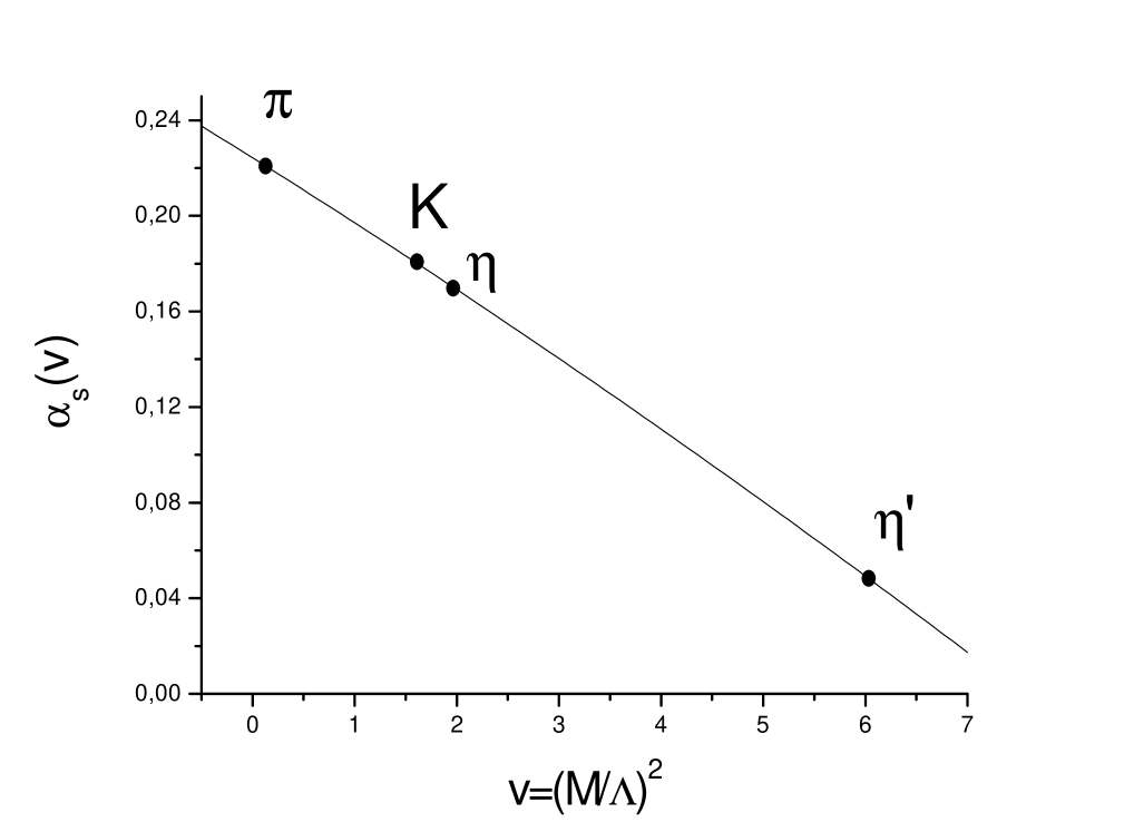
Figure 1: Pseudoscalar mesons. Parameters $\Lambda=390,~{}m_{u}=200,~{}~{}m_{s}=260,~{}~{}\theta=54^{\circ}.$ Decay constants $f_{\pi}=133,~{}~{}f_{K}=155$.

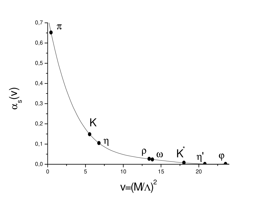
Figure 2: Pseudoscalar and vector mesons. Parameters $\Lambda=210,~{}m_{u}=180,~{}~{}m_{s}=230,~{}~{}\theta=54^{\circ}.$ Decay constants $f_{\pi}=80,~{}~{}f_{K}=107$.

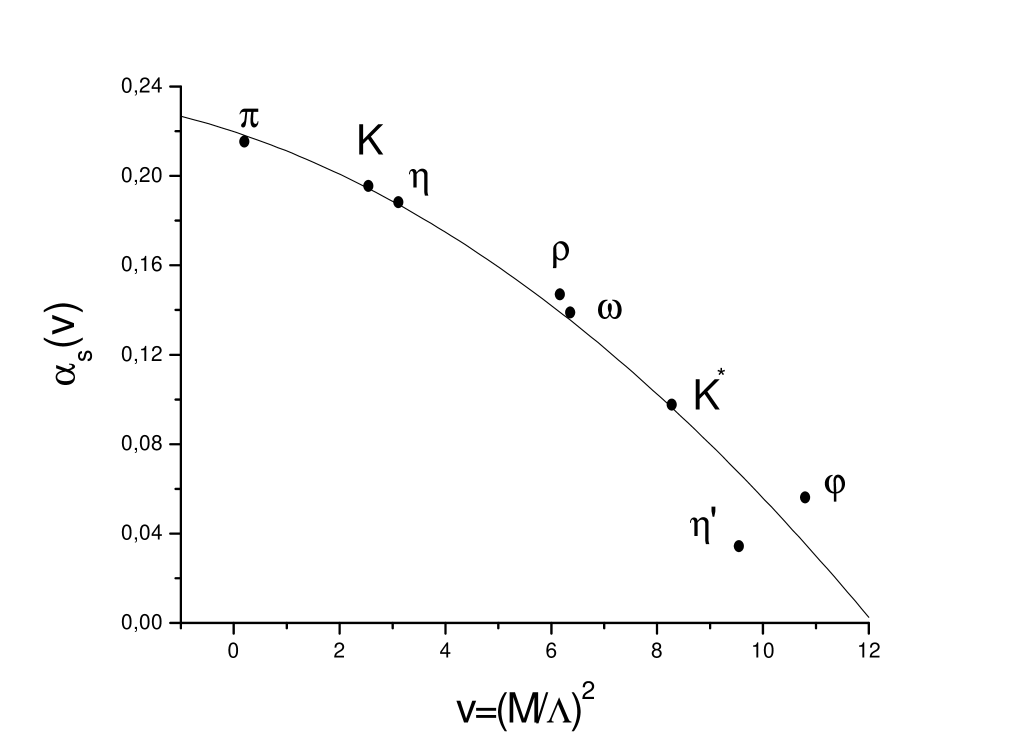
Figure 3: Pseudoscalar and vector mesons. Parameters $\Lambda=310,~{}m_{u}=130,~{}~{}m_{s}=240,~{}~{}\theta=64^{\circ}.$ Decay constants $f_{\pi}=131,~{}~{}f_{K}=172$.

References

• [1] D.Flamm and F.Schoeberl, Introduction to the Quark Model of Elementary Particles , Cordon & Breach Science Publ., N.Y., 1982.
• [2] Th.Feldmann, Int.J.of Mod.Phys., A15, 159 (2000).
• [3] P.Maris and C.D.Roberts, Int.J.of Mod.Phys., E12, 297 (2003).
• [4] R.T.Cahil and C.D.Roberts, Phys.Rev., D32, 2419 (1985);
C.D.Roberts, et  al, Phys.Rev., D49, 125 (1994).
• [5] M.Baldicchi and G.M.Prosperi, arXiv: hep-ph/0310213 v1 17 Oct 2003.
• [6] D.V.Schirkov, Theor.Math.Phys., 132, 484 (2002).
• [7] G.V.Efimov, On the Stability of QED and QCD, JINR, Dubna, P2-2003-226, 2003.
• [8] G.V.Efimov and M.A.Ivanov, The Quark Confinement Model of Hadrons, IOP Publishing Ltd, Bristol and Philadelphia, 1993.
• [9] G.V.Efimov and S.N.Nedelko, Phys.Rev., D51, 176 (1995); Phys.Rev., D54, 4483 (1996).
• [10] Ya.V.Burdanov and G.V.Efimov, Phys.Rev., D64, 014001 (2001).
• [11] G.V.Efimov and G.Ganbold, Phys.Rev., D65, 054012 (2002).
• [12] G.V.Efimov, On the Ladder Bethe-Salpeter Equation, Few Body Systems, 33, 199 (2003).
Refer to caption