July 2004 DESY 04-125
hep-ph/0407173
Proton Decay in Supersymmetric GUT Models

Abstract

The instability of protons is a crucial prediction of supersymmetric GUTs. We review the decay in minimal supersymmetric SU(5), which is dominated by dimension-five operators, and discuss the implications of the failure of Yukawa unification for the decay rate. In a consistent SU(5) model, where SU(5) relations among Yukawa couplings hold, the proton decay rate can be several orders of magnitude smaller than the present experimental bound. Finally, we discuss orbifold GUTs, where proton decay via dimension-five operators is absent. The branching ratios of dimension-six decay can significantly differ from those in four dimensions.
Keywords: baryon number violation; grand unified theory, orbifold; supersymmetry.
PACS Nos.: 11.10.Hi; 11.10.Kk; 12.10.-g; 12.60.Jv; 13.30.-a

The stability of protons has been a research topic for a long time [1], and exactly 50 years ago, the first experiments started to measure its lifetime [2] — although no mechanism was known that leads to proton decay. The situation changed when both baryon number violating processes were found in the Standard Model (SM) [3] and the idea of Grand Unification came up, where the SM is embedded in a simple gauge group [4]. Today, it is widely believed that protons will decay, even if they do so after a tremendously long time.

Grand Unified Theories predict proton decay and the unsuccessful search for decaying protons gives a strong constraint on GUT models. The first GUT model, minimal SU(5) [4], could already be excluded in the early 1980s. Recently, it was claimed that even its supersymmetric version [5] is excluded by the experimental limit on proton decay [6, 7]. In this review, we discuss these analyses and point out the crucial assumptions which have been made to analyze the dominant dimension-five operators. We will see that the problem of minimal supersymmetric SU(5) is less proton decay than the failure of Yukawa unification. Hence, we need a consistent model which explains the Yukawa couplings and we will see that a supersymmetric SU(5) model with minimal particle content cannot be excluded by proton decay [8].

Although such models are in agreement with the experimental limits on proton decay, the dimension-five operators are troublesome, as the Yukawa couplings must obey special relations among themselves. One would therefore like to avoid these operators. Orbifold GUTs offer an attractive solution, since they forbid dimension-five operators and, moreover, enable us to deal with the doublet-triplet splitting problem [9, 10, 11, 12]. Proton decay appears via dimension-six operators, which can lead to unusual final states depending on the localization of matter fields [13, 14]. We will illustrate this on the basis of a six-dimensional SO(10) model [15]. Hence, if proton decay is observed in the future, the measured branching ratios can make it possible to distinguish orbifold and four-dimensional GUTs.

1 Minimal supersymmetric SU(5)

We start this section by briefly describing the minimal supersymmetric SU(5) GUT model [5]. It contains three generations of chiral matter multiplets, $\mathsf{10}=(Q,u^{\text{\sc c}},e^{\text{\sc c}})$, $\mathsf{5}^{*}=(d^{\text{\sc c}},L)$, and a vector multiplet $A(\mathsf{24})$ which includes the twelve gauge bosons of the SM and twelve additional ones, the $X$ and $Y$ bosons. Because of their electric and color charges, the latter mediate proton decay via dimension-six operators. At the GUT scale, SU(5) is broken to ${\sf G_{\text{\sc sm}}=SU(3)\times SU(2)\times U(1)_{Y}}$ by an adjoint Higgs multiplet $\Sigma(\mathsf{24})$. A pair of quintets, $H(\mathsf{5})$ and $\makebox[9.12497pt][s]{$H$}\hskip 4.15619pt\overline{\makebox[6.64992pt][s]{ \vphantom{$H$} }}\hskip 4.56248pt(\mathsf{5}^{*})$, then breaks ${\sf G_{\text{\sc sm}}}$ to ${\sf SU(3)\times U(1)_{\text{em}}}$ at the electroweak scale. The superpotential is given by

$$\begin{split}W&=\tfrac{1}{2}m\operatorname{tr}\Sigma^{2}+\tfrac{1}{3}a\operatorname{tr}\Sigma^{3}+\lambda\makebox[9.12497pt][s]{$H$}\hskip 4.15619pt\overline{\makebox[6.64992pt][s]{ \vphantom{$H$} }}\hskip 4.56248pt\left(\Sigma+3\sigma\right)H+\tfrac{1}{4}Y_{1}^{ij}\mathsf{10}_{i}\,\mathsf{10}_{j}H+\sqrt{2}\,Y_{2}^{ij}\mathsf{10}_{i}\,\mathsf{5}^{*}_{j}\makebox[9.12497pt][s]{$H$}\hskip 4.15619pt\overline{\makebox[6.64992pt][s]{ \vphantom{$H$} }}\hskip 4.56248pt\end{split}$$ (1)

with $m={\cal O}\left(M_{\text{\sc gut}}\right)$. The adjoint Higgs multiplet,

$$\Sigma\left(\mathsf{24}\right)=\left(\begin{array}[]{cc}\Sigma_{8}&\Sigma_{(3,2)}\\ \Sigma_{(3^{*},2)}&\Sigma_{3}\end{array}\right)+\frac{1}{2\sqrt{15}}\left(\begin{array}[]{cc}2&0\\ 0&-3\end{array}\right)\Sigma_{24}\ ,$$ (6)

acquires the vacuum expectation value (VEV) $\left\langle\Sigma\right\rangle=\sigma\operatorname{diag}\left(2,2,2,-3,-3\right)$ so that the $X$ and $Y$ bosons become massive, whereas the SM particles remain massless. The components $\Sigma_{8}$ and $\Sigma_{3}$ of $\Sigma(\mathsf{24})$ both acquire the mass

$$M_{\Sigma}\equiv M_{8}=M_{3}=\tfrac{5}{2}m\ .$$ (7)

The pair of quintets, $H(\mathsf{5})$ and $\makebox[9.12497pt][s]{$H$}\hskip 4.15619pt\overline{\makebox[6.64992pt][s]{ \vphantom{$H$} }}\hskip 4.56248pt(\mathsf{5}^{*})$, contains the SM Higgs doublets, $H_{f}$ and $\makebox[9.12497pt][s]{$H$}\hskip 4.15619pt\overline{\makebox[6.64992pt][s]{ \vphantom{$H$} }}\hskip 4.56248pt_{\!f}$, which break $\mathsf{G_{\text{\sc sm}}}$, and color triplets, $H_{\text{\sc c}}$ and $\makebox[9.12497pt][s]{$H$}\hskip 4.15619pt\overline{\makebox[6.64992pt][s]{ \vphantom{$H$} }}\hskip 4.56248pt_{\text{\sc c}}$, respectively. To have massless Higgs doublets $H_{f}$ and $\makebox[9.12497pt][s]{$H$}\hskip 4.15619pt\overline{\makebox[6.64992pt][s]{ \vphantom{$H$} }}\hskip 4.56248pt_{\!f}$, while their color-triplet partners (leptoquarks) are kept super-heavy, the mass parameters of $H(\mathsf{5})$ and $\makebox[9.12497pt][s]{$H$}\hskip 4.15619pt\overline{\makebox[6.64992pt][s]{ \vphantom{$H$} }}\hskip 4.56248pt(\mathsf{5}^{*})$ have to be fine-tuned ${\cal O}\left(\frac{v_{\text{\sc ew}}}{\sigma}\right)\sim 10^{-13}$. This is called the doublet-triplet-splitting problem. The RGE analysis gives constraints on the masses of the new particles [7].

Expressed in terms of SM superfields, the Yukawa interactions are

$$\begin{split}W_{Y}=\;&Y_{u}^{ij}\,Q_{i}\,u^{\text{\sc c}}_{j}\,H_{f}+Y_{d}^{ij}\,Q_{i}\,d_{j}^{\text{\sc c}}\,\makebox[9.12497pt][s]{$H$}\hskip 4.15619pt\overline{\makebox[6.64992pt][s]{ \vphantom{$H$} }}\hskip 4.56248pt_{\!f}+Y_{e}^{ij}\,e_{i}^{\text{\sc c}}\,L_{j}\,\makebox[9.12497pt][s]{$H$}\hskip 4.15619pt\overline{\makebox[6.64992pt][s]{ \vphantom{$H$} }}\hskip 4.56248pt_{\!f}\\ &+\tfrac{1}{2}Y_{qq}^{ij}\,Q_{i}\,Q_{j}\,H_{\text{\sc c}}+Y_{ql}^{ij}\,Q_{i}\,L_{j}\,\makebox[9.12497pt][s]{$H$}\hskip 4.15619pt\overline{\makebox[6.64992pt][s]{ \vphantom{$H$} }}\hskip 4.56248pt_{\text{\sc c}}+Y_{ue}^{ij}\,u_{i}^{\text{\sc c}}\,e^{\text{\sc c}}_{j}\,H_{\text{\sc c}}+Y_{ud}^{ij}\,u_{i}^{\text{\sc c}}\,d_{j}^{\text{\sc c}}\,\makebox[9.12497pt][s]{$H$}\hskip 4.15619pt\overline{\makebox[6.64992pt][s]{ \vphantom{$H$} }}\hskip 4.56248pt_{\text{\sc c}}\ ,\end{split}$$ (8)

where

$$Y_{u}=Y_{qq}=Y_{ue} =Y_{1}\ , Y_{d}=Y_{e}=Y_{ql}=Y_{ud} =Y_{2}\ .$$ (9)

Apart from the SM couplings, there are four additional ones due to the colored leptoquarks. Integrating out those leptoquarks, two dimension five operators remain which lead to proton decay (Fig. 1) [16],

$$W_{5}=\frac{1}{M_{H_{\text{\sc c}}}}\left[\,\frac{1}{2}\,Y_{qq}^{ij}\,Y_{ql}^{km}\,\left(Q_{i}\,Q_{j}\right)\left(Q_{k}\,L_{m}\right)+Y_{ue}^{ij}\,Y_{ud}^{km}\,\left(u_{i}^{\text{\sc c}}\,e_{j}^{\text{\sc c}}\right)\left(u_{k}^{\text{\sc c}}\,d_{m}^{\text{\sc c}}\right)\,\right]\ ,$$ (10)

called the $LLLL$ and $RRRR$ operator. The scalars are transformed to their fermionic partners by exchange of a gauge or Higgs fermion. Neglecting external momenta, the triangle diagram factor reads, up to a coefficient $\kappa$ depending on the exchange particle,

$$\int\frac{d^{4}k}{i(2\pi)^{4}}\,\frac{1}{m_{1}^{2}-k^{2}}\,\frac{1}{m_{2}^{2}-k^{2}}\,\frac{1}{M-\hbox to0.0pt{\raisebox{1.0pt}{$\mskip 2.0mu/$}\hss}k}=\frac{1}{(4\pi)^{2}}f(M;m_{1},m_{2})\ ,$$ (11)

with

$$f(M;m_{1},m_{2})=\frac{M}{m_{1}^{2}-m_{2}^{2}}\left(\frac{m_{1}^{2}}{m_{1}^{2}-M^{2}}\,\ln\frac{m_{1}^{2}}{M^{2}}-\frac{m_{2}^{2}}{m_{2}^{2}-M^{2}}\,\ln\frac{m_{2}^{2}}{M^{2}}\right)\ ,$$ (12)

where $M$ and $m_{j}$ denote the gaugino and sfermion masses, respectively.

Figure 1: Proton Decay via dimension-five operators: They result from exchange of the leptoquarks followed by gaugino or higgsino dressing.

As a result of Bose statistics for superfields, the total anti-symmetry in the colour index requires that these operators are flavor non-diagonal [17]. The dominant decay mode is therefore $p\to K\bar{\nu}$. Since the dressing with gluinos and neutralinos is flavor diagonal, the chargino exchange diagrams are dominant [18, 19]. The wino exchange is related to the $LLLL$ operator and the charged higgsino exchange to the $RRRR$ operator, so that the coefficients of the triangle diagram factor are

$$\kappa_{\text{\sc l}} =2g^{2}\ , \kappa_{\text{\sc r}} =y\,y^{\prime}\ .$$ (13)

Here $y$ and $y^{\prime}$ denote the corresponding Yukawa couplings (cf. Fig. 1) and $g$ is the gauge coupling.

Let us sketch how to calculate the decay rate via dimension-five operators; for details see Ref. [8]. The Wilson coefficients $C_{5\text{\sc l}}=Y_{qq}Y_{ql}$ and $C_{5\text{\sc r}}=Y_{ue}Y_{ud}$ are evaluated at the GUT scale. Then they have to be evolved down to the SUSY breaking scale, leading to a short-distance renormalization factor $A_{s}$. Now the sparticles are integrated out, and the operators give rise to the effective four-fermion operators of dimension 6. The renormalization group procedure goes on to the scale of the proton mass, $m_{p}\sim 1\,$GeV, leading to a second, long-distance renormalization factor $A_{l}$ [20]. At 1 GeV, the link to the hadronic level is made using the chiral Lagrangean method [21]. Thus the decay width can be written as

$$\Gamma =\sum\left|\,{\cal K}_{\text{had}}\,A_{l}\,\frac{\kappa}{(4\pi)^{2}}f(M;m_{1},m_{2})\,A_{s}\,\frac{1}{M_{H_{\text{\sc c}}}}\,C_{5}\right|^{2}\ ,$$ (14)

where the sum includes all possible diagrams.

The decay width for the dominant channel $p\to K^{+}\bar{\nu}$ reads

$$\Gamma(p\to K^{+}\bar{\nu})=\dfrac{(m_{p}^{2}-m_{K}^{2})^{2}}{32\pi m_{p}^{3}f_{\pi}^{2}}\sum_{\nu}\left|\,C_{5}^{usd\nu}\,\frac{2m_{p}}{3m_{B}}D+\,C_{5}^{uds\nu}\,\left(1+\frac{m_{p}}{3m_{B}}(3F+D)\right)\right.\\ +\left.C_{5}^{dsu\nu}\,\left(1-\frac{m_{p}}{3m_{B}}(3F-D)\right)\right|^{2}\ .$$ (15)

Here, $m_{p}$ and $m_{K}$ denote the masses of the proton and kaon, respectively, and $f_{\pi}$ is the pion decay constant. $m_{B}$ is an average baryon mass according to contributions from diagrams with virtual $\Sigma$ and $\Lambda$ [21]. $D$ and $F$ are the symmetric and antisymmetric SU(3) reduced matrix elements for the axial-vector current.

According to the two Wilson coefficients, the coefficients $C_{5}$ split into two parts,

$$C_{5}=\beta\,C_{\text{\sc l}\text{\sc l}}+\alpha\,C_{\text{\sc r}\text{\sc l}}\ ,$$ (16)

with

$$C_{\text{\sc l}\text{\sc l}/\text{\sc r}\text{\sc l}}=\frac{1}{M_{H_{\text{\sc c}}}}\,C_{5\text{\sc l}/5\text{\sc r}}\,A_{s}\,A_{l}\,\frac{\kappa_{\text{\sc l}/\text{\sc r}}}{(4\pi)^{2}}f(M;m_{1},m_{2})$$ (17)

and the hadron matrix elements $\alpha$ and $\beta$ [22],

$$\alpha\,P_{\text{\sc l}}\,u_{p} =\epsilon_{\alpha\beta\gamma}\left\langle 0\!\left|\left(d_{\text{\sc r}}^{\alpha}\,u_{\text{\sc r}}^{\beta}\right)u_{\text{\sc l}}^{\gamma}\right|\!\,p\right\rangle\ , \beta\,P_{\text{\sc l}}\,u_{p} =\epsilon_{\alpha\beta\gamma}\left\langle 0\!\left|\left(d_{\text{\sc l}}^{\alpha}\,u_{\text{\sc l}}^{\beta}\right)u_{\text{\sc l}}^{\gamma}\right|\!\,p\right\rangle\ .$$ (18)

While the hadronic parameters are fairly known, the masses and mixings of the SUSY-particles are unknown. We know through their absence that they have to be heavier than ${\cal O}\,(100\,\text{GeV})$; on the other hand, they are expected not to be much heavier than ${\cal O}\,(1\,\text{TeV})$. Looking at the dressing diagram we notice that when taking the sfermions to be degenerate at a TeV, the triangle diagram factor (12) is given by

$$f(M;m)=\dfrac{M}{(M^{2}-m^{2})^{2}}\left(m^{2}-M^{2}-M^{2}\,\ln\frac{m^{2}}{M^{2}}\right)\;\xrightarrow{\;M\ll m\;}\;\frac{M}{m^{2}}\ .$$ (19)

The simplest case is to assume that the sfermions have masses of 1 TeV. An exception is often made for top squarks. Since the off-diagonal entries of the mass matrix are proportional to $m_{t}$, the mixing in the stop sector is expected to be large, with at least one eigenvalue much below 1 TeV. In analyses, one typically uses 400 GeV, 800 GeV, or 1 TeV for $m_{\tilde{t}}$. For the other sfermions, the mixings are neglected. The proton decay rate is further suppressed by light gauginos and higgsinos. Note that the experimental limit for charginos is $m_{\widetilde{\chi}^{\pm}}>67.7\,$GeV [23].

Since proton decay is dangerously large, the decoupling scenario [24] has also been studied, where the scalars of the first and second generation can be as heavy as 10 TeV [7]. Such an adjustment has been motivated by the supersymmetric flavor problem. In this scenario, proton decay via dimension-five operators is clearly dominated by the third generation.

Let us analyze the Wilson coefficients now. Minimal SU(5) predicts that the Yukawa couplings of down quarks and charged leptons are unified, as can be seen from Eqs. (9). While $m_{b}=m_{\tau}$ can be fulfilled at the GUT scale, the equalities fail for the first and second generation. Nevertheless, proton decay via dimension-five operators has been analyzed assuming

$$Y_{qq}=Y_{ue} =Y_{u}\ , Y_{ql}=Y_{ud} =Y_{d}\ .$$ (20)

Then the decay rate can be calculated as described above. Note, however, that the choices $Y_{ql}=Y_{ud}=Y_{e}$ or $Y_{ql}=Y_{d}$, $Y_{ud}=Y_{e}$ would be equally justified. As we shall see, this ambiguity strongly affects the proton decay rate.

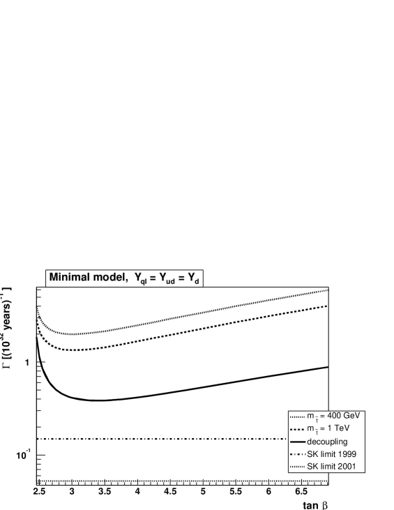
Figure 2: Decay rate $\Gamma(p\to K^{+}\bar{\nu})$ as function of $\tan\beta$ in minimal SU(5) with $Y_{ql}=Y_{ud}=Y_{d}$.

Fig. 2 shows the results of the following three cases: (i) all sfermions have masses of 1 TeV; (ii) $m_{\tilde{t}}$ is changed to 400 GeV; (iii) decoupling scenario, where the scalars of the first and second generation have masses of 10 TeV. The dash-dotted line represents the experimental limit $\tau=6.7\times 10^{32}$ years as given by the Super-Kamiokande experiment [23, 26], the dotted line is the newer limit $\tau=1.9\times 10^{33}$ years [27].

The Wilson coefficients are proportional to $\tan\beta+\frac{1}{\tan\beta}$ and $(\tan\beta+\frac{1}{\tan\beta})^{2}$, where $\tan\beta$ is the ratio of the vacuum expectation values of the Higgs doublets $H_{f}$ and $\makebox[9.12497pt][s]{$H$}\hskip 4.15619pt\overline{\makebox[6.64992pt][s]{ \vphantom{$H$} }}\hskip 4.56248pt_{\!f}$. Clearly low values are preferred for obtaining a low decay rate; on the other hand, the top Yukawa coupling becomes non-perturbative for $\tan\beta\lesssim 2.5$.

As already mentioned, it is possible to constrain the leptoquark mass using the RGEs. These constraints depend strongly on the Higgs representations, therefore we choose the most conservative value $M_{H_{\text{\sc c}}}=M_{\text{GUT}}=2\times 10^{16}\,\text{GeV}$ in order to study whether the experimental limit already rules out this model.

The decay rate in Fig. 2 is always above the experimental limit, which led to the claim that minimal SU(5) is excluded [6, 7]. But as already discussed, there is no compelling reason for the assumption $Y_{ql}=Y_{ud}=Y_{d}$! In order to illustrate the strong dependence of the decay rate on flavor mixing and therefore on Yukawa unification, let us study the case

$$Y_{qq}=Y_{ue} =Y_{u}\ , Y_{ql}=Y_{ud} =Y_{e}\ .$$ (21)

Then the mixing matrix $U_{u}^{\dagger}\,U_{d}\equiv V_{\text{\sc ckm}}$, which appears in the Wilson coefficients, is replaced by ${\cal M}=U_{u}^{\dagger}\,U_{e}$. Note that the mixing matrix in $Y_{u}$ or $Y_{d}$ is still given by $V_{\text{\sc ckm}}$. Since $Y_{d}\not=Y_{e}$, the masses and mixing of quarks and leptons are different and ${\cal M}$ is undetermined.

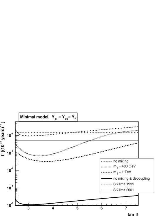
Figure 3: Decay rate $\Gamma(p\to K^{+}\bar{\nu})$ as a function of $\tan\beta$ with $Y_{ql}=Y_{ud}=Y_{e}$.

We first ignore mixing, i. e. ${\cal M}=\mathbbm{1}$, and calculate the decay rate; the results are shown in Fig. 3. Without mixing, only scalars of the first and second generation take part, so the decay rate is significantly reduced in the decoupling scenario where the triangle diagram factor (12) changes by almost two orders of magnitude.

If, moreover, we take ${\cal M}$ arbitrarily, it is possible to push the decay width below the experimental limit even for smaller sfermion masses. In the case $m_{\tilde{t}}=400$ GeV, this is only possible for small values of $\tan\beta$.

The fact that a sufficiently low decay rate can be found illustrates the dependence on flavor mixing and therefore the uncertainty due to the failure of Yukawa unification. Minimal supersymmtric SU(5) can only be excluded by the mismatch between the Yukawa couplings of down quarks and charged leptons as non-supersymmetric SU(5) is excluded by the failure of gauge unification.

2 Consistent supersymmetric SU(5)

Minimal supersymmetric SU(5) is inconsistent due to the failure of Yukawa unification, thus additional interactions are required which account for the difference of down quark and charged lepton masses. Such interactions are conveniently parameterized by higher dimensional operators, which are naturally expected as a result of interactions at a higher scale, where the GUT model is extended to a more fundamental theory. In particular, the GUT scale is only about two orders below the Planck scale.

Including possible terms up to order $1/M_{\text{Pl}}$, the superpotential reads [28]

$$W =\tfrac{1}{2}m\operatorname{tr}\Sigma^{2}+\tfrac{1}{3}a\operatorname{tr}\Sigma^{3}+b\frac{(\operatorname{tr}\Sigma^{2})^{2}}{M_{\text{Pl}}}+c\frac{\operatorname{tr}\Sigma^{4}}{M_{\text{Pl}}}$$

$$\quad+\frac{1}{4}\,\epsilon_{abcde}\left(Y_{1}^{ij}\mathsf{10}_{i}^{ab}\mathsf{10}_{j}^{cd}H^{e}+f_{1}^{ij}\mathsf{10}_{i}^{ab}\mathsf{10}_{j}^{cd}\frac{\Sigma^{e}_{f}}{M_{\text{Pl}}}H^{f}+f_{2}^{ij}\mathsf{10}_{i}^{ab}\mathsf{10}_{j}^{cf}\,H^{d}\frac{\Sigma^{e}_{f}}{M_{\text{Pl}}}\right)$$

$$\quad+\sqrt{2}\left(Y_{2}^{ij}\makebox[9.12497pt][s]{$H$}\hskip 4.15619pt\overline{\makebox[6.64992pt][s]{ \vphantom{$H$} }}\hskip 4.56248pt_{a}\mathsf{10}_{i}^{ab}\mathsf{5}^{*}_{jb}+h_{1}^{ij}\makebox[9.12497pt][s]{$H$}\hskip 4.15619pt\overline{\makebox[6.64992pt][s]{ \vphantom{$H$} }}\hskip 4.56248pt_{a}\frac{\Sigma^{a}_{b}}{M_{\text{Pl}}}\mathsf{10}_{i}^{bc}\mathsf{5}^{*}_{jc}+h_{2}^{ij}\makebox[9.12497pt][s]{$H$}\hskip 4.15619pt\overline{\makebox[6.64992pt][s]{ \vphantom{$H$} }}\hskip 4.56248pt_{a}\mathsf{10}_{i}^{ab}\frac{\Sigma_{b}^{c}}{M_{\text{Pl}}}\mathsf{5}^{*}_{jc}\right)\ .$$ (22)

Now the masses of $\Sigma_{3}$ and $\Sigma_{8}$ are no longer identical, affecting the constraint on the leptoquark mass [28].

The Yukawa couplings are then given by

$$\begin{split}Y_{u}&=Y_{1}+3\frac{\sigma}{M_{\text{Pl}}}f_{1}^{S}+\frac{1}{4}\frac{\sigma}{M_{\text{Pl}}}\left(3f_{2}^{S}+5f_{2}^{A}\right)\ ,\\ Y_{d}&=Y_{2}-3\frac{\sigma}{M_{\text{Pl}}}h_{1}+2\frac{\sigma}{M_{\text{Pl}}}h_{2}\ ,\\ Y_{e}&=Y_{2}-3\frac{\sigma}{M_{\text{Pl}}}h_{1}-3\frac{\sigma}{M_{\text{Pl}}}h_{2}\ .\end{split}$$ (23)

Here $\sigma/M_{\text{Pl}}\sim{\cal O}\left(10^{-2}\right)$, and $S$ and $A$ denote the symmetric and antisymmetric parts of the matrices. Thus the three Yukawa matrices, which are related to masses and mixing angles at $M_{Z}$ by the RGEs, are determined by six matrices. From Eqn. (23) one reads off

$$Y_{d}-Y_{e}=5\frac{\sigma}{M_{\text{Pl}}}h_{2}\ ,$$ (24)

hence, the failure of Yukawa unification is naturally accounted for by the presence of $h_{2}$. Note that no additional field is introduced to obtain this relation; it just arises from corrections ${\cal O}\left(\sigma/M_{\text{Pl}}\right)$.

Let us study the effect of those higher-dimensional operators on the Wilson coefficients. It is instructive to express the couplings in terms of the quark and charged lepton Yukawa couplings and the additional matrices $f$ and $h$,

$$Y_{qq}=Y_{qq}^{S}=Y_{ue}^{S} =Y_{u}^{S}-5\frac{\sigma}{M_{\text{Pl}}}\left(f_{1}^{S}+\frac{1}{4}f_{2}^{S}\right), Y_{ql} =Y_{e}+5\frac{\sigma}{M_{\text{Pl}}}h_{1}\ ,$$ (25)

$$Y_{ue}^{A} =Y_{u}^{A}-\frac{5}{2}\,\frac{\sigma}{M_{\text{Pl}}}f_{2}^{A}\ , Y_{ud} =Y_{d}+5\frac{\sigma}{M_{\text{Pl}}}h_{1}\ .$$ (26)

Note that $Y_{ql}-Y_{ud}=Y_{e}-Y_{d}$, which means that $Y_{ql}$ and $Y_{ud}$ cannot be zero at the same time. Nevertheless, proton decay via dimension-five operators can be avoided if both $C_{5L}=Y_{qq}Y_{ql}$ and $C_{5R}=Y_{ue}Y_{ud}$ vanish. For this purpose the couplings have to fulfill the relations

$$f_{1}^{S}+\frac{1}{4}f_{2}^{S} =\frac{M_{\text{Pl}}}{5\,\sigma}\,Y_{u}^{S}\ , f_{2}^{A} =\frac{2}{5}\,\frac{M_{\text{Pl}}}{\sigma}\,Y_{u}^{A}\ .$$ (27)

This is only possible if we allow the (3,3)-component of $f_{1}$ and $f_{2}$ to be ${\cal O}\left(\frac{M_{\text{Pl}}}{\sigma}\right)\gg 1$. But even if we restrict ourselves to ‘natural matrices’, i. e. couplings up to ${\cal O}\left(1\right)$, we can considerably reduce the decay amplitudes. We will illustrate this with two simple examples where either the $RRRR$ or the $LLLL$ contribution vanishes at the GUT scale.

We assume that $Y_{qq}$, $Y_{ql}$, $Y_{ue}$ and $Y_{ud}$ are all diagonal by a suitable choice of matrices. The simplest form of $Y_{qq}$ and $Y_{ue}$ is then

$$Y_{qq}=Y_{ue} =\operatorname{diag}\left(0,0,y_{t}\right)\ ,$$ (28)

where $y_{t}$ is the top Yukawa coupling at $M_{\text{\sc gut}}$. In the first model, we spread $Y_{e}-Y_{d}$ such that

$$Y_{ud} =\operatorname{diag}\left(0,y_{s}-y_{\mu},y_{b}-y_{\tau}\right)\ , Y_{ql} =\operatorname{diag}\left(y_{e}-y_{d},0,0\right)\ .$$ (29)

Clearly $C_{5R}^{ijkm}=Y_{ue}^{ij}\ Y_{ud}^{km}$ is zero whenever a particle of the first generation takes part. Since at least one particle of the first generation is needed, the $RRRR$ contribution vanishes completely. After RGE evolution, this simple structure of Wilson coefficients changes slightly, but as shown in Fig. 4, the decay amplitude is always well below the experimental limit — in the case $m_{\tilde{t}}=1$ TeV even more than two orders of magnitude. Here, we restrict ourselves to the cases where the sfermion masses are not heavier than 1 TeV.

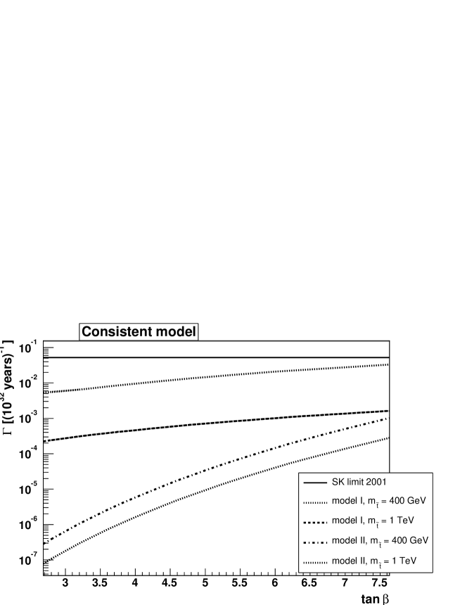
Figure 4: Decay rate $\Gamma(p\to K^{+}\bar{\nu})$ as function of $\tan\beta$ in the consistent models.

If we choose the matrices $Y_{ql}$ and $Y_{ud}$ as

$$Y_{ud} =\operatorname{diag}\left(y_{d}-y_{e},y_{s}-y_{\mu},y_{b}\right)\ , Y_{ql} =\operatorname{diag}\left(0,0,y_{\tau}\right)\ ,$$ (30)

the $LLLL$ contribution vanishes at $M_{\text{\sc gut}}$ because now $C_{5L}^{ijkm}=Y_{qq}^{ij}\ Y_{ql}^{km}$ is only different from zero for $i=j=k=m=3$, but the decay has to be non-diagonal. Only the $RRRR$ contribution with a low absolute value remains. After renormalization, this contribution is still dominated by third generation scalars, and the $LLLL$ operator contributes only via $p\to K\bar{\nu}_{\tau}$. In this case, the decay rate is even smaller (Fig. 4). Furthermore, due to the smaller (3,3)-component of $h_{1}$ compared to the first model, it can easily be used for higher values of $\tan\beta$.

We have seen that higher-dimensional operators can reduce the proton decay rate by several orders of magnitude and make it consistent with the experimental upper bound. This impressing fact leads to the question, whether there is any mechanism which would naturally lead to the required relations among Yukawa couplings. We can think of two possibilities, to start with some ad-hoc textures as a result of an unknown additional symmetry [29] or to extend the analysis to another group, in order to obtain additional symmetry restrictions. SO(10), however, does not restrict the contributions from the higher-dimensional operators [30]. Thus it is more promising to consider theories, where the dimension-five operators are generically absent.

3 Orbifold GUTs

In orbifold GUTs, the GUT gauge symmetry is realized in more than four space-time dimensions and broken to the standard model by compactification on an orbifold, utilizing boundary conditions that violate the GUT symmetry [9, 10, 11, 12]. As a consequence, the GUT and electroweak scale are separated in an elegant way and the dimension-five operators are absent [10, 11]. Furthermore, in case of SO(10), the breaking to $G_{\text{\sc sm}}$ via the Higgs mechanism requires large Higgs representations and the path is not unique. Here, orbifold GUTs provide an attractive solution as well, as orbifold symmetry breaking can simplify the breaking pattern.

Figure 5: The three SO(10) subgroups at the corresponding fixed points (branes) of the orbifold $T^{2}/{\mathbbm{Z}}_{2}\times{\mathbbm{Z}}_{2}^{\prime}\times{\mathbbm{Z}}_{2}^{\prime\prime}$.

We consider a 6D SUSY SO(10) model compactified on a torus with three ${\mathbbm{Z}}_{2}$ parities [31]. The first ${\mathbbm{Z}}_{2}$ breaks only $N=1$ 6D SUSY to $N=1$ 4D SUSY, the remaining ones SO(10) as well, namely to ${\sf G_{\text{\sc gg}}=SU(5)\times U(1)}$ and ${\sf G_{\text{\sc ps}}=SU(4)\times SU(2)\times SU(2)}$ [32], respectively. Then the zero modes belong to the intersection of the two symmetric subgroups, ${\sf G_{\text{\sc sm}}\times U(1)^{\prime}}$. The physical region is a ‘pillow’, corresponding to the two compact dimensions, with four fixed points as corners, where the unbroken subgroups are SO(10), ${\sf G_{\text{\sc ps}}}$, ${\sf G_{\text{\sc gg}}}$, and flipped SU(5) [33] (Fig. 5).

The field content is as follows [34]: The matter fields are located on the branes, whereas the gauge fields, six 10-dimensional Higgs representations and two combinations ${\sf 16\oplus\makebox[10.00003pt][s]{$\sf 16$}\hskip 4.37495pt\overline{\makebox[6.99994pt][s]{ \vphantom{$\sf 16$} }}\hskip 5.00002pt}$, are bulk fields. The matter fields include the 10 and ${\sf 5}^{*}$ of SU(5) plus a singlet, the right-handed neutrino. With this setup, both the irreducible and reducible 6D gauge anomalies vanish.

The main idea to generate fermion mass matrices is to locate the three sequential 16-plets on the three branes where SO(10) is broken to its three GUT subgroups, namely $\psi_{1}$ at $O_{\text{\sc gg}}$, $\psi_{2}$ at $O_{\text{fl}}$ and $\psi_{3}$ at $O_{\text{\sc ps}}$. The three ‘families’ are then separated by distances large compared to the cutoff scale $M_{*}={\cal O}\left(10^{17}\,\text{GeV}\right)$, where the theory becomes strongly coupled. Thus they can only have diagonal Yukawa couplings with the bulk Higgs fields, direct mixings are exponentially suppressed. The brane fields mix with the bulk field zero modes. These mixings take place only among left-handed leptons and right-handed down-quarks, which leads to a characteristic pattern of mass matrices.

The mass terms read

$$W=d_{\alpha}m^{d}_{\alpha\beta}d^{\text{\sc c}}_{\beta}+e^{\text{\sc c}}_{\alpha}m^{e}_{\alpha\beta}e_{\beta}+n^{\text{\sc c}}_{\alpha}m^{D}_{\alpha\beta}\nu_{\beta}+u_{i}m^{u}_{ij}u^{\text{\sc c}}_{j}+\tfrac{1}{2}n^{\text{\sc c}}_{i}m^{N}_{ij}n^{\text{\sc c}}_{j}\ .$$ (31)

Here $m^{u}$ and $m^{N}$ are diagonal $3\times 3$ matrices but due to the mixing with the bulk field zero modes, $m^{d}$, $m^{e}$ and $m^{D}$ are $4\times 4$ matrices with a lopsided structure,

$$\frac{1}{\tan{\beta}}\,m^{u}\sim\frac{v_{u}M_{*}}{v_{B-L}^{2}}\,m^{N} \sim\operatorname{diag}\left(\mu_{1},\mu_{2},\mu_{3}\right),$$ (32)

$$\frac{1}{\tan{\beta}}\,m^{D}\sim m^{d}\sim m^{e} \sim\left(\begin{array}[]{cccc}\mu_{1}&0&0&\tilde{\mu}_{1}\\ 0&\mu_{2}&0&\tilde{\mu}_{2}\\ 0&0&\mu_{3}&\tilde{\mu}_{3}\\ \widetilde{M}_{1}&\widetilde{M}_{2}&\widetilde{M}_{3}&\widetilde{M}_{4}\end{array}\right);$$ (37)

$\mu_{i}$ and $\tilde{\mu}_{j}$ are ${\cal O}\,(v_{\text{\sc ew}})$, whereas $\widetilde{M}_{\alpha}$ are of the order of the compactification scale.

The fermion masses and mixings agree well with the data within coefficients ${\cal O}\left(1\right)$ in the case $\mu_{1,2}\to 0$ [34]. Note that while $m_{\tau}\simeq m_{b}$, the muon and electron masses can be easily accommodated because $\mu_{2}^{d}$ and $\mu_{2}^{e}$ are not related by a flipped SU(5) mass relation.

While the mixings for the left-handed down quarks and right-handed charged leptons are small so that their diagonalization matrices read

$$U^{d}_{\text{\sc l}}=V_{\text{\sc ckm}}\simeq U^{e}_{\text{\sc r}}\ ,$$ (38)

those for the right-handed down quarks and left-handed charged leptons are large. For those, the diagonalization matrices are given by

$$U^{d}_{\text{\sc r}}\sim U^{e}_{\text{\sc l}}\simeq\left(\begin{array}[]{cccc}-\frac{\widetilde{M}_{2}}{\widetilde{M}_{12}}&\frac{\widetilde{M}_{1}\left(\tilde{\mu}_{3}\widetilde{M}_{3}-\mu_{3}\widetilde{M}_{4}\right)}{\bar{\mu}\,\widetilde{M}\,\widetilde{M}_{12}}&-\frac{\widetilde{M}_{1}\left(\tilde{\mu}_{3}\widetilde{M}_{4}+\mu_{3}\widetilde{M}_{3}\right)}{\bar{\mu}\,\widetilde{M}^{2}}&\frac{\widetilde{M}_{1}}{\widetilde{M}}\\ \rule[-11.38109pt]{0.0pt}{28.45274pt}\frac{\widetilde{M}_{1}}{\widetilde{M}_{12}}&\frac{\widetilde{M}_{2}\left(\tilde{\mu}_{3}\widetilde{M}_{3}-\mu_{3}\widetilde{M}_{4}\right)}{\bar{\mu}\,\widetilde{M}\,\widetilde{M}_{12}}&-\frac{\widetilde{M}_{2}\left(\tilde{\mu}_{3}\widetilde{M}_{4}+\mu_{3}\widetilde{M}_{3}\right)}{\bar{\mu}\,\widetilde{M}^{2}}&\frac{\widetilde{M}_{2}}{\widetilde{M}}\\ \rule[-14.22636pt]{0.0pt}{28.45274pt}0&-\frac{\tilde{\mu}_{3}}{\bar{\mu}}\frac{\widetilde{M}_{12}}{\widetilde{M}}&-\frac{\tilde{\mu}_{3}\widetilde{M}_{3}\widetilde{M}_{4}-\mu_{3}\left(\widetilde{M}_{1}^{2}+\widetilde{M}_{2}^{2}+\widetilde{M}_{4}^{2}\right)}{\bar{\mu}\,\widetilde{M}^{2}}&\frac{\widetilde{M}_{3}}{\widetilde{M}}\\ 0&\frac{\mu_{3}}{\bar{\mu}}\frac{\widetilde{M}_{12}}{\widetilde{M}}&\frac{\tilde{\mu}_{3}\left(\widetilde{M}_{1}^{2}+\widetilde{M}_{2}^{2}+\widetilde{M}_{3}^{2}\right)-\mu_{3}\widetilde{M}_{3}\widetilde{M}_{4}}{\bar{\mu}\,\widetilde{M}^{2}}&\frac{\tilde{M}_{4}}{\widetilde{M}}\end{array}\right)$$ (43)

up to a two-dimensional mixing matrix for the second and third generation, which can be neglected for the purpose of proton decay. In Eqn. (43), $\bar{\mu}_{3}$ is ${\cal O}\left(\mu_{3},\tilde{\mu}_{3}\right)$, furthermore $\widetilde{M}_{12}=\sqrt{\widetilde{M}_{1}^{2}+\widetilde{M}_{2}^{2}}$ and $\widetilde{M}^{2}=\sum_{\alpha}\widetilde{M}_{\alpha}^{2}$.

The up-quarks are confined to one fixed point each, in particular the up quark is located on the Georgi-Glashow one. Therefore dimension-six proton decay can arise via the exchange of the SU(5) $X$ and $Y$ bosons as in the four-dimensional case,

$${\mathscr{L}}_{\text{eff}} =-\frac{g_{5}^{2}}{M_{V}^{2}}\;\epsilon_{\alpha\beta\gamma}\left[\makebox[7.0797pt][s]{$e^{c}$}\hskip 3.64488pt\overline{\makebox[5.83183pt][s]{ \vphantom{$e^{c}$} }}\hskip 3.53984pt_{\!j}\makebox[8.14801pt][s]{$u^{c}$}\hskip 3.91196pt\overline{\makebox[6.25914pt][s]{ \vphantom{$u^{c}$} }}\hskip 4.074pt_{\!\alpha i}\,Q_{\beta i}\,Q_{\gamma,j}-\makebox[7.6283pt][s]{$d^{c}$}\hskip 3.78204pt\overline{\makebox[6.05127pt][s]{ \vphantom{$d^{c}$} }}\hskip 3.81415pt_{\!\alpha k}\makebox[8.14801pt][s]{$u^{c}$}\hskip 3.91196pt\overline{\makebox[6.25914pt][s]{ \vphantom{$u^{c}$} }}\hskip 4.074pt_{\!\beta i}\,Q_{\gamma i}\,L_{k}\right]+\text{h.c.}\,.$$ (44)

The analysis of these operators is analogous to the dimension-five case; for details see Ref. [15]. Contrary to the 4D case, we have to take into account the presence of the Kaluza-Klein tower of the vector bosons $V=\left(X,Y\right)$ with masses

$$M_{V}^{2}(n,m)=\frac{(2n+1)^{2}}{R_{5}^{2}}+\frac{(2m)^{2}}{R_{6}^{2}}\ .$$ (45)

Furthermore, the KK modes interact more strongly by a factor of $\sqrt{2}$ due to their bulk normalization [11].

The sum over the KK modes is logarithmically divergent. Since the theory is only valid below the scale $M_{*}$, we restrict the sum to masses $M_{V}(n,m)\leq M_{*}$. In the case $R_{5}=R_{6}=1/M_{c}$, we obtain

$$\frac{1}{(M_{V}^{\text{eff}})^{2}}=2\sum_{n,m=0}^{\infty}\frac{1}{M_{V}^{2}(n,m)}\simeq\frac{\pi}{4\,M_{c}^{2}}\,\left(\ln\left(\frac{M_{*}}{M_{c}}\right)+2.3\right)\ .$$ (46)

As we will see below, $M_{c}$ is constrained by the experimental limit of the dominant decay mode $p\to e^{+}\pi^{0}$ yielding $M_{*}/M_{c}\simeq 12$.

Due to the parities and the ${\sf SO(10)}$ breaking pattern, the coupling of the gauge bosons is not universal any more, in contrast to the 4D case. Their wavefunctions vanish on the fixed points $O_{\text{\sc ps}}$ and $O_{\text{fl}}$ so that no coupling arises via the kinetic term with the second and third generation. The couplings to the bulk states are irrelevant since these are embedded in full SU(5) multiplets together with massive KK modes, thus the interaction always mixes the light states with the heavy ones [13, 14].

Altogether, the operators for the decay via $X$ and $Y$ bosons read

$${\mathscr{L}}_{\text{eff}}=\frac{g_{5}^{2}}{(M_{V}^{\text{eff}})^{2}}\left[\,\makebox[7.69376pt][s]{$d^{\text{\sc c}}$}\hskip 3.7984pt\overline{\makebox[6.07745pt][s]{ \vphantom{$d^{\text{\sc c}}$} }}\hskip 3.84688pt_{\!\!\alpha,l}\left(U^{d\top}_{\text{\sc r}}\right)_{l1}\makebox[8.21347pt][s]{$u^{\text{\sc c}}$}\hskip 3.92831pt\overline{\makebox[6.28532pt][s]{ \vphantom{$u^{\text{\sc c}}$} }}\hskip 4.10674pt_{\!\beta 1}\left(u_{\gamma 1}\left(U^{e}_{\text{\sc l}}\right)_{1j}e_{j}-d_{\gamma m}\left(U^{d}_{\text{\sc l}}\right)_{1m}\left(U^{\nu}_{\text{\sc l}}\right)_{1j}\nu_{j}\right)\right.\\ +\left.2\,\makebox[7.14516pt][s]{$e^{\text{\sc c}}$}\hskip 3.66125pt\overline{\makebox[5.85802pt][s]{ \vphantom{$e^{\text{\sc c}}$} }}\hskip 3.57257pt_{\!k}\left(U^{e\top}_{\text{\sc r}}\right)_{k1}\makebox[8.21347pt][s]{$u^{\text{\sc c}}$}\hskip 3.92831pt\overline{\makebox[6.28532pt][s]{ \vphantom{$u^{\text{\sc c}}$} }}\hskip 4.10674pt_{\!\!\alpha 1}\,d_{\beta m}\left(U^{d}_{\text{\sc l}}\right)_{1m}u_{\gamma 1}\vphantom{\left(u_{\gamma 1}\left(U^{e}_{\text{\sc l}}\right)_{1j}\right)}\right]\epsilon_{\alpha\beta\gamma}+\text{h.c.}$$ (47)

with the fermions in their mass eigenstates.

We start with the simplest case of $U_{\text{\sc r}}^{d}=U_{\text{\sc l}}^{e}$ and degenerate masses $\widetilde{M}_{\alpha}$ in the limit $\tilde{\mu}_{3}=\mu_{3}$, which we denote case I. In this case, the state $d_{R1}$ has no strange-component and we obtain

$${\mathscr{L}}_{\text{eff}}=\frac{g_{5}^{2}}{(M_{V}^{\text{eff}})^{2}}\;\epsilon_{\alpha\beta\gamma}\left[2\,V_{ud}^{2}\,\makebox[7.14516pt][s]{$e^{\text{\sc c}}$}\hskip 3.66125pt\overline{\makebox[5.85802pt][s]{ \vphantom{$e^{\text{\sc c}}$} }}\hskip 3.57257pt\,\makebox[8.21347pt][s]{$u^{\text{\sc c}}_{\alpha}$}\hskip 3.92831pt\overline{\makebox[6.28532pt][s]{ \vphantom{$u^{\text{\sc c}}_{\alpha}$} }}\hskip 4.10674pt\,d_{\beta}\,u_{\gamma}+\frac{1}{2}\,\makebox[7.69376pt][s]{$d^{\text{\sc c}}_{\alpha}$}\hskip 3.7984pt\overline{\makebox[6.07745pt][s]{ \vphantom{$d^{\text{\sc c}}_{\alpha}$} }}\hskip 3.84688pt\,\makebox[8.21347pt][s]{$u^{\text{\sc c}}_{\beta}$}\hskip 3.92831pt\overline{\makebox[6.28532pt][s]{ \vphantom{$u^{\text{\sc c}}_{\beta}$} }}\hskip 4.10674pt\,u_{\gamma}\,e+2\,V_{ud}V_{us}\,\makebox[8.51437pt][s]{$\mu^{\text{\sc c}}$}\hskip 4.00354pt\overline{\makebox[6.40569pt][s]{ \vphantom{$\mu^{\text{\sc c}}$} }}\hskip 4.25719pt\,\makebox[8.21347pt][s]{$u^{\text{\sc c}}_{\alpha}$}\hskip 3.92831pt\overline{\makebox[6.28532pt][s]{ \vphantom{$u^{\text{\sc c}}_{\alpha}$} }}\hskip 4.10674pt\,d_{\beta}\,u_{\gamma}\vphantom{\sum_{j=1}^{3}}\right.\\ +2\,V_{ud}V_{us}\,\makebox[7.14516pt][s]{$e^{\text{\sc c}}$}\hskip 3.66125pt\overline{\makebox[5.85802pt][s]{ \vphantom{$e^{\text{\sc c}}$} }}\hskip 3.57257pt\,\makebox[8.21347pt][s]{$u^{\text{\sc c}}_{\alpha}$}\hskip 3.92831pt\overline{\makebox[6.28532pt][s]{ \vphantom{$u^{\text{\sc c}}_{\alpha}$} }}\hskip 4.10674pt\,s_{\beta}\,u_{\gamma}+2\,V_{us}^{2}\,\makebox[8.51437pt][s]{$\mu^{\text{\sc c}}$}\hskip 4.00354pt\overline{\makebox[6.40569pt][s]{ \vphantom{$\mu^{\text{\sc c}}$} }}\hskip 4.25719pt\,\makebox[8.21347pt][s]{$u^{\text{\sc c}}_{\alpha}$}\hskip 3.92831pt\overline{\makebox[6.28532pt][s]{ \vphantom{$u^{\text{\sc c}}_{\alpha}$} }}\hskip 4.10674pt\,s_{\beta}\,u_{\gamma}\\[-4.0pt] -\left.\sum_{j=1}^{3}\frac{1}{\sqrt{2}}\,\left(U^{\nu}_{L}\right)_{1j}\,\makebox[8.21347pt][s]{$u^{\text{\sc c}}_{\alpha}$}\hskip 3.92831pt\overline{\makebox[6.28532pt][s]{ \vphantom{$u^{\text{\sc c}}_{\alpha}$} }}\hskip 4.10674pt\,\makebox[7.69376pt][s]{$d^{\text{\sc c}}_{\beta}$}\hskip 3.7984pt\overline{\makebox[6.07745pt][s]{ \vphantom{$d^{\text{\sc c}}_{\beta}$} }}\hskip 3.84688pt\,\left\{V_{ud}\,d_{\gamma}\,+V_{us}\,s_{\gamma}\vphantom{\frac{1}{2}}\right\}\,\nu_{j}\right]+\text{h.c.}$$ (48)

The numerical results for the branching ratios are shown in Table 1.

Additional operators can arise at any brane from couplings which contain the derivative along the extra dimensions of the locally vanishing gauge bosons [14]. Their contribution is suppressed with respect to the standard operators [15]; the coefficients, however, are undetermined. For $c_{5}=c_{6}=1$, the corrections for the listed branching ratios are less than 3%.

decay channel	Branching Ratios [%]
	6D SO(10)		4D SU(5)
	case I	case II
$e^{+}\pi^{0}$	75	71	54
$\mu^{+}\pi^{0}$	4	5	< 1
$\bar{\nu}\,\pi^{+}$	19	23	27
$e^{+}K^{0}$	1	1	< 1
$\mu^{+}K^{0}$	< 1	< 1	18
$\bar{\nu}\,K^{+}$	< 1	< 1	< 1

Table 1: Resulting branching ratios and comparision with ${\sf SU(5)}\times{\sf U(1)}_{F}$.

To make a comparison with ordinary 4D GUT models, we consider two SU(5) models described in Refs. [35, 36], where we assume that some mechanism suppresses or avoids the proton decay arising from dimension-five operators. These models make use of the Froggatt-Nielsen mechanism [38] where a global ${\sf U(1)}_{F}$ symmetry is broken spontaneously by the vev of a gauge singlet field $\Phi$ at a high scale. Then the Yukawa couplings arise from the non-renormalizable operators,

$$h_{ij}=g_{ij}\left(\frac{\left\langle\Phi\right\rangle}{\Lambda}\right)^{Q_{i}+Q_{j}}\ .$$ (49)

Here, $g_{ij}$ are couplings $\mathcal{O}\left(1\right)$ and $Q_{i}$ are the charges of the various fermions. Particularly interesting is the case with a ‘lopsided’ family structure, where the chiral ${\sf U(1)}_{F}$ charges are different for the ${\sf 5}^{*}$ and ${\sf 10}$ of the same family.

The difference between the 6D SO(10) and 4D SU(5) models is most noticeable in the channel $p\to\mu^{+}K^{0}$. This is due to the absence of second and third generation weak eigenstates in the current-current operators and the vanishing (12)-component. Hence the decay $p\to\mu^{+}K^{0}$ is doubly Cabibbo suppressed. This effect is a direct consequence of the localization of the ‘first generation’ to the Georgi-Glashow brane.

Let us now consider the general case, where the $\widetilde{M}^{d,e}$ are not degenerate and where $\mu_{3}$ and $\tilde{\mu}^{d,e}_{3}$ differ as well. From Eqn. (43) we see that strange component in $d^{\text{\sc c}}_{1}$ does not vanish anymore, but it is smaller than the bottom component. We have studied several cases whose results agree remarkably well. As an illustration, consider the case where $\tilde{\mu}^{d}_{3}=2\mu_{3}$ and $\tilde{\mu}^{e}_{3}=3\mu_{3}$, with non-degenerate heavy masses $\widetilde{M}^{d}_{1}:\widetilde{M}^{d}_{2}:\widetilde{M}^{d}_{3}:\widetilde{M}^{d}_{4}=\frac{1}{2}:\frac{1}{\sqrt{2}}:\frac{1}{\sqrt{2}}:1$ and $\widetilde{M}^{e}_{1}:\widetilde{M}^{e}_{2}:\widetilde{M}^{e}_{3}:\widetilde{M}^{e}_{4}=\frac{1}{2}:\frac{1}{\sqrt{2}}:1:\frac{1}{2}$ (case II). The branching ratios are listed in Table 1; the differences between the two cases are indeed small.

The most striking difference between the 4D and 6D case is the decay channel $p\to\mu^{+}K^{0}$, which is suppressed by about two orders of magnitude in the 6D model with respect to 4D models. It is therefore important to determine an upper limit for this channel in the 6D model. Varying the mass parameters in the range $\widetilde{M}^{d,e}_{\alpha}/\widetilde{M}=0.1-1$ and $\tilde{\mu}_{3}^{d,e}/\mu_{3}=0.1-10$, we find

$$\frac{\Gamma(p\to\mu^{+}K^{0})}{\Gamma(p\to e^{+}\pi^{0})}\lesssim 5\,\%\ ,$$ (50)

one order of magnitude smaller than in the four-dimensional case. Note that in 5D orbifold GUTs, this channel is typically enhanced because the first generation is located in the bulk [13, 14].

Finally, we can derive the lower limit on the compactification scale from the decay width of the dominant channel $p\to e^{+}\pi^{0}$ yielding $M_{c}\geq 9\times 10^{15}\,\text{GeV}$, roughly half of the 4D GUT scale.

4 Conclusion

Supersymmetric GUTs provide a beautiful framework for theories beyond the Standard Model. The simplest model, minimal SU(5), is inconsistent due to the failure of down quark and charged lepton masses to unify. The decay amplitude therefore depends strongly on flavor mixing. A consistent SU(5) model requires additional interactions, which are conveniently parameterized by higher dimensional operators. These operators can reduce the proton decay rate by several orders of magnitude, hence proton decay does not rule out consistent supersymmetric SU(5) models.

Nevertheless, it is interesting to consider models where dimension-five operators are absent; this is generically the case in orbifold GUTs. We discussed a 6D SO(10) model, where the position of the matter fields on the different branes leads to a characteristic pattern of mass matrices. The branching ratios differ significantly from predictions of 4D GUTs, which can make it possible to distinguish orbifold and four dimensional GUTs. Furthermore, proton decay restricts the compactification scale $M_{c}$ to be ${\cal O}\left(M_{\text{\sc gut}}^{\text{4D}}\right)$.

If proton decay is observed in the future, there will be only a few events. The dominance of the channel $p\to\bar{\nu}K^{+}$, however, would strongly point at dimension-five operators, whereas $p\to e^{+}\pi^{0}$ refers to dimension-six decay. In the latter case, the absence of the process $p\to\mu^{+}K^{0}$ would disfavor the naïve GUT model in four dimensions and test the idea that the different generations are spatially separated.

Acknowledgements

I am grateful to W. Buchmüller, L. Covi and D. Emmanuel-Costa for collaboration and I would like to thank them as well as A. Brandenburg for a careful reading of the manuscript.

References

-
[1]
E. C. G. Stückelberg, Helv. Phys. Acta 11 (1938) 299;
E. P. Wigner, Proc. Am. Phil. Soc. 93 (1949) 521; Proc. Natl. Acad. Sci. 38 (1952) 449. -
[2]
F. Reines, C. L. Cowan and M. Goldhaber, Phys. Rev.
96 (1954) 1157;
H. S. Gurr, W. R. Kropp, F. Reines and B. Meyer, Phys. Rev. 158 (1967) 1321. - [3] G. ’t Hooft, Phys. Rev. Lett. 37 (1976) 8.
- [4] H. Georgi and S. L. Glashow, Phys. Rev. Lett. 32 (1974) 438.
-
[5]
S. Dimopoulos and H. Georgi, Nucl. Phys. B 193 (1981) 150;
N. Sakai, Z. Phys. C 11 (1981) 153. - [6] T. Goto and T. Nihei, Phys. Rev. D 59 (1999) 115009, hep-ph/9808255.
- [7] H. Murayama and A. Pierce, Phys. Rev. D 65 (2002) 055009, hep-ph/0108104.
- [8] D. Emmanuel-Costa and S. Wiesenfeldt, Nucl. Phys. B 661 (2003) 62, hep-ph/0302272.
- [9] Y. Kawamura, Prog. Theor. Phys. 103 (2000) 613, hep-ph/9902423; 105 (2001) 999, hep-ph/0012125.
- [10] G. Altarelli and F. Feruglio, Phys. Lett. B 511 (2001) 257, hep-ph/0102301.
- [11] L. J. Hall and Y. Nomura, Phys. Rev. D 64 (2001) 055003, hep-ph/0103125.
- [12] A. Hebecker and J. March-Russell, Nucl. Phys. B 613 (2001) 3, hep-ph/0106166.
- [13] Y. Nomura, Phys. Rev. D 65 (2002) 085036, hep-ph/0108170.
- [14] A. Hebecker and J. March-Russell, Phys. Lett. B 539 (2002) 119, hep-ph/0204037.
- [15] W. Buchmüller, L. Covi, D. Emmanuel-Costa and S. Wiesenfeldt, JHEP 409 (2004) 4, hep-ph/0407070.
-
[16]
N. Sakai and T. Yanagida, Nucl. Phys. B 197
(1982) 533;
S. Weinberg, Phys. Rev. D 26 (1982) 287. - [17] S. Dimopoulos, S. Raby and F. Wilczek, Phys. Lett. B 112 (1982) 133.
- [18] P. Nath, A. H. Chamseddine and R. Arnowitt, Phys. Rev. D 32 (1985) 2348.
- [19] J. Hisano, H. Murayama and T. Yanagida, Nucl. Phys. B 402 (1993) 46.
- [20] J. R. Ellis, D. V. Nanopoulos and S. Rudaz, Nucl. Phys. B 202 (1982) 43.
-
[21]
M. Claudson, M. B. Wise and L. J. Hall, Nucl. Phys. B 195 (1982) 297.
S. Chadha and M. Daniel, Nucl. Phys. B 229 (1983) 105. - [22] S. J. Brodsky, J. R. Ellis, J. S. Hagelin and C. T. Sachrajda, Nucl. Phys. B 238 (1984) 561.
- [23] K. Hagiwara et al., Phys. Rev. D 66 (2002) 010001.
-
[24]
M. Dine, A. Kagan and S. Samuel, Phys. Lett. B
243 (1990) 250;
S. Dimopoulos and G. F. Giudice, Phys. Lett. B 357 (1995) 573, hep-ph/9507282;
A. Pomarol and D. Tommasini, Nucl. Phys. B 466 (1996) 3, hep-ph/9507462;
A. G. Cohen, D. B. Kaplan and A. E. Nelson, Phys. Lett. B 388 (1996) 588, hep-ph/9607394. - [25] B. Bajc, P. F. Perez and G. Senjanovic, Phys. Rev. D 66 (2002) 075005, hep-ph/0204311.
- [26] Y. Hayato et al., Phys. Rev. Lett. 83 (1999) 1529, hep-ex/9904020.
- [27] K. S. Ganezer, Int. J. Mod. Phys. A 16S1B (2001) 855.
- [28] B. Bajc, P. F. Perez and G. Senjanovic, hep-ph/0210374.
-
[29]
P. Nath, Phys. Rev. Lett. 76 (1996) 2218,
hep-ph/9512415; Phys. Lett. B 381 (1996) 147, hep-ph/9602337;
Z. Berezhiani, Z. Tavartkiladze and M. Vysotsky, hep-ph/9809301. - [30] W. Buchmüller, D. Emmanuel-Costa and S. Wiesenfeldt (in preparation).
-
[31]
T. Asaka, W. Buchmüller and L. Covi, Phys. Lett. B 523 (2001) 199,
hep-ph/0108021;
L. J. Hall, Y. Nomura, T. Okui and D. R. Smith, Phys. Rev. D 65 (2002) 035008, hep-ph/0108071. - [32] J. C. Pati and A. Salam, Phys. Rev. D 10 (1974) 275.
-
[33]
S. M. Barr, Phys. Lett. B 112 (1982) 219;
J. P. Derendinger, J. E. Kim and D. V. Nanopoulos, Phys. Lett. B 139 (1984) 170. - [34] T. Asaka, W. Buchmüller and L. Covi, Phys. Lett. B 563 (2003) 209, hep-ph/0304142.
- [35] T. Yanagida, J. Sato, Nucl. Phys. Proc. Suppl. 77 (1999) 293, hep-ph/9809307.
- [36] G. Altarelli and F. Feruglio, New J. Phys. 6 (2004) 106, hep-ph/0405048.
-
[37]
Y. Achiman and M. Richter, Phys. Lett. B 523
(2001) 304, hep-ph/0107055;
J. Ellis, D. V. Nanopoulos and J. Walker, Phys. Lett. B 550 (2002) 99, hep-ph/0205336;
P. F. Pérez, Phys. Lett. B 595 (2004) 476, hep-ph/0403286. - [38] C. D. Froggatt and H. B. Nielsen, Nucl. Phys. B 147 (1979) 277.