Collinear Photon Exchange in the Beam Normal Polarization
Asymmetry of Elastic Electron-Proton Scattering

Abstract

The parity-conserving single-spin beam asymmetry of elastic electron-proton scattering is induced by an absorptive part of the two-photon exchange amplitude. We demonstrate that this asymmetry has logarithmic and double-logarithmic enhancement due to contributions of hard collinear quasi-real photons. An optical theorem is used to evaluate the asymmetry in terms of the total photoproduction cross section on the proton, predicting its magnitude at a few parts per million for high electon beam energies and small scattering angles. At fixed 4-momentum transfers, the asymmetry is rising logarithmically with increasing electron beam energy, following the high-energy diffractive behavior of total photoproduction cross section on the proton.

I Introduction

It has been known for a long time ST1 ; Barut ; Ru that the two photon exchange (TPE) mechanism can generate the single-spin normal asymmetry (SSNA) of electron scattering due to a nonzero imaginary part of the TPE amplitude $A_{2\gamma}$,

$$A_{n}=\frac{2A_{Born}\Im(A^{*}_{2\gamma})}{|A_{Born}|^{2}}\,$$ (1)

where symbol $\Im$ denotes the imaginary (absorptive) part. The one-photon-exchange amplitude $A_{Born}$ is purely real due to time-reversal invariance of electromagnetic interactions.

The first calculations of the TPE effect on the proton aam predicted the magnitude of beam SSNA at the level of a few parts per million (ppm). The effect appears to be small due to two suppression factors combined: $\alpha=1/137$, since the effect is higher-order in the electromagnetic interaction, and the electron mass $m_{e}$ arising due to electron helicity flip. The predictions of Ref.aam which correspond only to elastic intermediate proton state are in qualitative agreement with experimental data from MIT/Bates Wells and they were reproduced later in Ref.Mark .

However, the main theoretical problem in description of the TPE amplitude on the proton is a large uncertainty in the contribution of the inelastic hadronic intermediate states. In Ref.Mark the beam SSNA at large momentum transfers was estimated at the level of one ppm, using the partonic picture developed in Ref.Afanas for TPE effects but not related to the electron helicity flip.

Current experiments designed for parity-violating electron scattering allow to measure the beam asymmetry with a fraction of ppm accuracy Maas ; E158 ; PViol and may also provide data on the parity-conserving beam SSNA. In fact, such measurements are needed because beam SSNA is a source of systematic corrections in the measurements of parity-violating observables.

It was noted in aam that while considering excitation of inelastic intermediate hadronic states, the beam SSNA (Eq.(11) of Ref.aam ), after factoring out the electron mass, has an enhancement when at least one of the photons in the TPE loop diagram is collinear to its parent electron. It is interesting that this effect did not appear for the target SSNA. Similar behaviour of the beam SSNA in the nucleon resonance region was observed also in Pasquini where authors used a phenomenological model (MAID) for single-pion electroproduction.

In this paper we demonstrate that collinear photon exchange in the TPE amplitude results in single- and double-logarithmic enhancement of the beam SSNA, whereas such enhancement does not take place for the target SSNA (with unpolarized electrons) and spin correlations caused by longitudinal polarization of the scattering electrons. For large electron energies and small scattering angles, we use an optical theorem to relate the nucleon Compton amplitude to the total photoproduction cross section and obtain a simple analytic formula for the beam SSNA in this kinematics.

II Leptonic and hadronic tensors

First, we write the formula for SSNA in terms of rank-3 leptonic and hadronic tensors which appear in the interference between the Born and TPE amplitudes as shown in Fig.1.

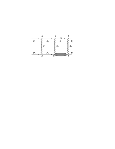
Figure 1: Interference between the Born and the TPE box diagrams in elastic e-p scattering that determines SSNA.

$$A_{n}=\frac{-i\alpha Q^{2}}{\pi^{2}D(s,Q^{2})}\int\frac{d^{3}k}{2E_{k}}\frac{L_{\mu\alpha\beta}H_{\mu\alpha\beta}}{q_{1}^{2}q_{2}^{2}}\ ,$$ (2)

where $Q^{2}=-q^{2}$, $k(E_{k})$ is the 3-momentum (energy) of the intermediate on-mass-shell electron in the TPE box diagram, $q_{1}$ and $q_{2}$ are the 4-momenta of the intermediate photons, $q_{1}-q_{2}=q$. The factor $Q^{2}/D(s,Q^{2})$ in Eq.(2) is due to the squared Born amplitude, namely,

$$D(s,Q^{2}) = \frac{Q^{4}}{2}\big{(}F_{1}+F_{2}\big{)}^{2}+[(s-M^{2})^{2}-$$ (3)

$$Q^{2}s]\Big{(}F_{1}^{2}+\frac{Q^{2}}{4M^{2}}F_{2}^{2}\Big{)},$$

where $F_{1}(F_{2})$ is the Dirac (Pauli) proton form factor, $M$ is the proton mass and $s=(k_{1}+p_{1})^{2}.$ Our sign convention for the beam asymmetry follows from the definition of the normal vector with respect to the electron scattering plane: ${\bf{k}_{1}}\times{\bf{k}_{2}}.$

Using the above notation, we have

$$L_{\mu\alpha\beta}=\frac{1}{4}Tr(\hat{k}_{2}+m_{e})\gamma_{\mu}(\hat{k}_{1}+m_{e})(1-\gamma_{5}\hat{\xi^{e}})\gamma_{\beta}(\hat{k}+m_{e})\gamma_{\alpha}\ ,$$ (4)

and

$$H_{\mu\alpha\beta}=\frac{1}{4}Tr(\hat{p}_{2}+M)\Gamma_{\mu}(\hat{p}_{1}+M)(1-\gamma_{5}\hat{\xi^{p}})\Im T_{\beta\alpha}\ ,$$ (5)

where $m_{e}$ is the electron mass, $\xi^{e}(\xi^{p})$ is the polarization 4-vector of the electron beam (proton target), $\Gamma_{\mu}=\gamma_{\mu}(F_{1}+F_{2})-(p_{1\mu}+p_{2\mu})F_{2}/(2M)$, and $T_{\beta\alpha}$ is in general a non-forward proton Compton tensor that describes any possible hadronic intermediate states in the TPE amplitude. In accordance with Eq.(2) the single-spin normal asymmetry probes the imaginary part of contraction of the leptonic and hadronic tensors defined by Eqs.(4) and (5), respectively. These tensors satisfy the conditions

$$q_{\mu}L_{\mu\alpha\beta}=q_{2\alpha}L_{\mu\alpha\beta}=q_{1\beta}L_{\mu\alpha\beta}=0,$$

$$q_{\mu}H_{\mu\alpha\beta}=q_{2\alpha}H_{\mu\alpha\beta}=q_{1\beta}H_{\mu\alpha\beta}=0,$$ (6)

separately for spin–independent and spin–dependent parts, as follows from gauge invariance of electromagnetic interactions.

After some algebra we arrive at the following expression for the model-independent leptonic tensor

$$L_{\mu\alpha\beta}=L^{(un)}_{\mu\alpha\beta}+L^{(pol)}_{\mu\alpha\beta}\ ,$$ (7)

where the spin–independent part is

$$L^{(un)}_{\mu\alpha\beta}=\frac{1}{2}q_{1}^{2}(g_{\mu\beta}k_{2\alpha}-g_{\mu\alpha}k_{2\beta})-\frac{1}{2}q_{2}^{2}(g_{\mu\beta}k_{1\alpha}-g_{\mu\alpha}k_{1\beta})$$

$$-k_{\mu}[k_{1}k_{2}]_{\alpha\beta}+\frac{1}{2}g_{\alpha\beta}(q_{1}^{2}k_{2\mu}+q_{2}^{2}k_{1\mu}-q^{2}k_{\mu})+$$ (8)

$$\frac{1}{2}q^{2}(g_{\mu\alpha}k_{\beta}+g_{\mu\beta}k_{\alpha})+k_{2\mu}(kk_{1})_{\alpha\beta}+k_{1\mu}(kk_{2})_{\alpha\beta}\ ,$$

$$[ab]_{\alpha\beta}=a_{\alpha}b_{\beta}-a_{\beta}b_{\alpha}\ ,\ \ (ab)_{\alpha\beta}=a_{\alpha}b_{\beta}+a_{\beta}b_{\alpha}\ ,$$

and the spin–dependent part is given by

$$L^{(pol)}_{\mu\alpha\beta}=im_{e}\bigg{[}-g_{\alpha\beta}(\mu qq_{2}\xi^{e})+k_{\beta}(\mu\alpha q\xi^{e})+k_{\alpha}(\mu\beta q\xi^{e})$$

$$+\xi^{e}_{\mu}(\alpha\beta qq_{2})+(\xi^{e}k_{2})(\mu\alpha\beta q_{1})+k_{2\mu}(\alpha\beta q_{1}\xi^{e})+$$

$$k_{1\mu}(\alpha\beta q_{2}\xi^{e})+\frac{1}{2}q^{2}(\mu\alpha\beta\xi^{e})\bigg{]}\ ,$$ (9)

$$(abcd)\equiv\epsilon_{\nu\lambda\rho\sigma}a_{\nu}b_{\lambda}c_{\rho}d_{\sigma}\ ,$$

where the on-shell condition $k^{2}_{\mu}=m_{e}^{2}$ was used for the intermediate electron 4-momentum.

If one of photon in the box diagram is collinear to its parent electron, for example,

$$q_{1}=xk_{1},\ \ x=\frac{W^{2}-M^{2}}{s-M^{2}}\ ,$$ (10)

where $W^{2}$ is the squared invariant mass of the intermediate hadronic system, leptonic tensor can be written as

$$L_{\mu\alpha\beta}=\frac{1-x}{x}q_{1\beta}L^{B}_{\mu\alpha}+im_{e}xL^{\xi}_{\mu\alpha\beta}\ .$$ (11)

The tensor $L^{B}_{\mu\alpha}$ coincides with the Born one of elastic electron–proton scattering and

$$L^{\xi}_{\mu\alpha\beta}=-g_{\alpha\beta}(\mu qk_{1}\xi^{e})+\frac{q^{2}}{2}(\mu\alpha\beta\xi^{e})+\xi^{e}_{\mu}(\alpha\beta qk_{1})+$$

$$(\xi^{e}k_{2})(\mu\alpha\beta k_{1})+k_{2\mu}(\alpha\beta k_{1}\xi^{e})+k_{1\mu}(\alpha\beta k_{2}\xi^{e})\ .$$ (12)

In the case of longitudinal polarization of the electron beam $(\xi^{e}_{mu}=k_{1\mu}/m_{e})$ the tensor $L^{\xi}_{\mu\alpha\beta}$ is zero. Therefore, we expect no contribution from considered kinematics to the target SSNA or to longitudinal-spin correlations because any gauge invariant hadronic tensor has to give zero after contracting with $q_{1\beta}$ (see Eq.(6)).

In the case of the normal polarized electron beam

$$\xi^{e}_{\mu}=\frac{2(\mu k_{1}p_{1}q)}{\sqrt{Q^{2}[(s-M^{2})^{2}-Q^{2}s]}}\ .$$ (13)

tensor $L^{\xi}_{\mu\alpha\beta}$ is not zero and the considered collinear photon kinematics contributes with essential logarithmic enhancement.

Therefore, conservation of the electromagnetic current that follows from gauge invariance (Eq.(II)) is the reason why the collinear intermediate photons appear in the TPE contribution to the beam SSNA, but not to the target SSNA. By analogy, we do not anticipate contributions from collinear-photon exchange in unpolarized electron-proton scattering, parity-conserving and parity-violating asymmetries due to longitudinal electron polarization the normal polarization of leptons is not involved.

Let us consider the hadronic tensor. Small values of $Q^{2}$ correspond to the forward limit of nucleon virtual Compton amplitude $T_{\beta\alpha}$. On the other hand, because $q_{1}^{2}$ and $q_{2}^{2}$ are also small in the collinear photon limit, we can relate the forward Compton amplitude to the total photoproduction cross section by real photons.

A general form of the Compton tensor $T_{\beta\alpha}$ in terms of 18 independent invariant amplitudes that are free from kinematical singularities and zeros was derived in Ref.Tarrach . Among these amplitudes we choose the ones that contribute at the limit $q^{2}\to 0$ and $q_{1}^{2}\to 0.$ It automatically constrains virtuality of the second photon to $q_{2}^{2}\to 0$. There is only one structure that contains the tensor $g_{\alpha\beta}$ and does not die off under the considered conditions. It reads Tarrach

$$T_{\beta\alpha}=\Big{[}-(\bar{p}\bar{q})^{2}g_{\alpha\beta}-(q_{1}q_{2})\bar{p}_{\alpha}\bar{p}_{\beta}+(\bar{p}\bar{q})(\bar{p}_{\beta}q_{1\alpha}+$$

$$\bar{p}_{\alpha}q_{2\beta})\Big{]}A(q_{1}^{2},q_{2}^{2},q^{2},W^{2}),$$ (14)

$$\bar{p}=\frac{1}{2}(p_{1}+p_{2}),\ \ \bar{q}=\frac{1}{2}(q_{1}+q_{2})\ .$$

It can be verified that $T_{\beta\alpha}$ defined by the above equation satisfies the conditions $T_{\beta\alpha}q_{1\beta}=T_{\beta\alpha}q_{2\alpha}=0.$

The normalization convention is chosen such that the imaginary part of the quantity $(W^{2}-M^{2}-q_{1}q_{2})^{2}A(W^{2},q^{2}=0,q_{1}^{2}=q_{2}^{2})$ is connected with the inelastic proton structure function $W_{1}(W^{2},q_{1}^{2})$ by the following relation

$$(W^{2}-M^{2}-q_{1}q_{2})^{2}\Im A(W^{2},q^{2}=0,q_{1}^{2}=q_{2}^{2})=$$ (15)

$$\frac{\pi}{M}W_{1}(W^{2},q_{1}^{2})\ ,$$

and $W_{1}$, in turn, defines the total photoproduction cross section Lev as

$$W_{1}(W^{2},0)=\frac{W^{2}-M^{2}}{8\pi^{2}\alpha}\sigma^{\gamma p}_{tot}(W^{2})\ .$$ (16)

Keeping in mind that the main contribution to the beam SSNA arises from collinear photon kinematics, we can combine relations (5), (14) and (15) and write hadronic tensor in the following form

$$H_{\mu\alpha\beta}=2\pi W_{1}\Big{(}F_{1}-\tau F_{2}\Big{)}p_{1\mu}\Big{(}-g_{\alpha\beta}-\frac{2[p_{1}q]_{\alpha\beta}}{W^{2}-M^{2}}\Big{)}\ ,$$

$$\tau=\frac{Q^{2}}{4M^{2}}\ .$$ (17)

When writing this last expression we neglect the terms containing $(q_{1}q_{2}),$ which lead to the contribution of the order $Q^{2}/W^{2}$ in the beam SSNA.

It may seem at first that in the considered limiting case of very small $Q^{2}$ one can omit all terms proportional to $q$ in the hadronic tensor. But such approximation is valid only for the symmetric part of $T_{\beta\alpha}$ with respect to the indexes $\alpha$ and $\beta.$ The reason is that the corresponding symmetric part of the leptonic tensor (see Eq.(II)) contains the momentum transfer $q$, and keeping it in the symmetric part of hadronic tensor leads after contraction to additional small terms of the order at least $Q^{2}/W^{2}.$ On the other hand, the antisymmetric part of leptonic tensor contains terms which do not include the momentum $q.$ Therefore, the antisymmetric part in Eq.(17) has to be retained because it contributes at the same order with respect to $Q^{2}/W^{2}.$ Note, however, that this antisymmetric part of the hadronic tensor is not related to the polarized nucleon structure functions, but it comes about as a consequence of the gauge-invariant structure of Eq.(II) even for a spinless hadronic target.

III Master formula

To compute the contraction of tensors in Eq.(2) we use the relations

$$-g_{\alpha\beta}p_{1\mu}L^{(pol)}_{\mu\alpha\beta}=2im_{e}[(p_{1}qq_{1}\xi^{e})+(k_{1}p_{1}q\xi^{e})],$$

$$-[p_{1}q]_{\alpha\beta}p_{1\mu}L^{(pol)}_{\mu\alpha\beta}=im_{e}(u-s)(p_{1}qq_{1}\xi^{e}),$$

$s+q^{2}+u=2M^{2}$ , which are valid for the normal beam polarization $((\xi^{e}k_{1})=(\xi^{e}k_{2})=(\xi^{e}p_{1})=(\xi^{e}p_{2})=0)$, and the explicit form of 4–vector $\xi^{e}$ given by Eq.(13). Then we arrive at

$$L^{(pol)}_{\mu\alpha\beta}H_{\mu\alpha\beta}=$$ (18)

$$im_{e}\sqrt{Q^{2}}\Big{(}F_{1}-\tau F_{2}\Big{)}\frac{(W^{2}-M^{2})(s-W^{2})}{4\pi\alpha}\sigma_{T}(W^{2},q_{1}^{2})\ ,$$

where $\sigma_{T}(W^{2},q_{1}^{2})$ is the total photoproduction cross section with the transverse virtual photons. When integrating with respect to $W^{2}$ we take $\sigma_{T}(W^{2},q_{1}^{2})\rightarrow\sigma^{\gamma p}_{tot}(W^{2})$ and assume $\sigma^{\gamma p}_{tot}(W^{2})$ to be constant with energy ($\approx$ 0.1 mb, according to Ref.pdg ).

Taking into account Eqs. (2) and (18) one can write the beam SSNA at small values of $Q^{2}$ as

$$A_{n}^{e}=\frac{m_{e}\sqrt{Q^{2}}\sigma^{\gamma p}_{tot}}{4\pi^{3}}\frac{F_{1}-\tau F_{2}}{F_{1}^{2}+\tau F_{2}^{2}}I\ ,$$ (19)

$$I=\int\frac{d^{3}k}{2E_{k}}\frac{(W^{2}-M^{2})(W^{2}-s)}{(s-M^{2})^{2}}\frac{Q^{2}}{q_{1}^{2}q_{2}^{2}}\ .$$

Here and further we use notation where $E_{k1},\ E_{k}(\bf k_{1},\ \bf k)$ are the energies (3-momenta) of the initial and intermediate electron, respectively. The angular integration in Eq. (19) can be done by introducing the Feynman parameter

$$\int\frac{d\Omega_{k}}{q_{1}^{2}q_{2}^{2}}=\int\limits_{0}^{1}dy\int\frac{d\Omega_{k}}{[-2m_{e}^{2}+2(kk_{y})]^{2}}\ ,$$

$$k_{y}=yk_{1}+(1-y)k_{2}=(E_{k1};y{\bf{k}_{1}}+(1-y){\bf{k}_{2}}),$$

$$(kk_{y})=E_{k1}E_{k}-2k|{\bf{k}_{y}}|\cos{\theta_{y}},\ \ d\Omega_{k}=d\Phi d\cos{\theta_{y}}\ .$$

Integration over $d\Omega_{k}$ and Feynman parameter $y$ is straightforward, leading to

$$I=\frac{\pi}{2}\int_{m_{e}}^{E_{k1}}\frac{dE_{k}}{k}z(z-1)L,\ L=\frac{1}{K}\log\frac{2K+1}{2K-1}$$ (20)

where $z=E_{k}/E_{k1}$, and

$$\ L=\frac{1}{K}\log\frac{2K+1}{2K-1}\ ,K=\sqrt{\frac{1}{4}+\eta},\ \eta=\frac{m_{e}^{2}(E_{k1}-E_{k})^{2}}{Q^{2}k^{2}}\ .$$

We extended the upper limit up to $E_{k1}$ because the difference between the value of $E_{k}$ at inelastic threshold of pion production (when $W^{2}=(m_{\pi}+M)^{2}$) and $E_{k1}$ is negligible at large $s.$

To calculate the integral in Eq.(20), we note first that the region where $k\simeq 0$ does not contribute because of the factor of $L$. For this reason we can change integration with respect to $E_{k}$ by integration over $k.$ Then we divide the integration region into the following two parts, $0<k<\lambda m_{e}$ and $\lambda m_{e}<k<E_{k1}$, and choose the auxiliary parameter $\lambda$ in such a way that

$$\lambda>>1,\ \lambda m_{e}<<E_{k1}<<\sqrt{Q^{2}}\lambda\ .$$ (21)

In the first region we can neglect $E_{k}$ as compared with $E_{k1}$ and write the corresponding contribution in the form

$$I_{1}=\pi\int\limits_{0}^{\lambda m_{e}}\frac{dk}{k}L$$ (22)

$$=\frac{2m_{e}}{\sqrt{Q^{2}}}\int\limits_{0}^{\lambda\sqrt{Q^{2}}/2E_{k1}}\frac{2\pi dz}{\sqrt{1+z^{2}}}\log(z+\sqrt{1+z^{2}})$$

$$={\cal O}(\frac{2m_{e}}{\sqrt{Q^{2}}}).$$

We see that the contribution from the first region is negligible, therefore we can choose zero for the lower limit of integration in $I_{2}$. In the second region the quantity $\eta$ that enters $L$ is small and we have

$$I_{2}=\pi\int\limits_{0}^{1}dz(z-1)\Big{(}\log\frac{Q^{2}}{m_{e}^{2}}+2\log\frac{z}{1-z}\Big{)}\ .$$ (23)

The integration in Eq.(23) gives

$$I_{2}=\frac{\pi}{2}\Big{(}-\log\frac{Q^{2}}{m_{e}^{2}}+2\Big{)}\ .$$

In the sum $I_{1}+I_{2}$ we arrive at the following master formula that defines the beam SSNA for small values of $Q^{2}$ and takes into account contributions from intermediate collinear photons in the TPE box diagrams

$$A_{n}^{e}=\frac{m_{e}\sqrt{Q^{2}}\sigma^{\gamma p}_{tot}}{8\pi^{2}}\frac{F_{1}-\tau F_{2}}{F_{1}^{2}+\tau F_{2}^{2}}\Big{(}-\log\frac{Q^{2}}{m_{e}^{2}}+2\Big{)}\ .$$ (24)

One can see that at fixed values of $Q^{2}$ the beam SSNA does not depend on the beam energy if the total photoproduction cross section is energy-independent. This remarkable property of small-angle beam SSNA follows from unitarity of the scattering matrix and does not rely on a specific model of nucleon structure.

IV Numerical results and conclusion

The master formula for beam SSNA Eq.(24) neglects possible $Q^{2}$ dependence of the invariant form factor of the nucleon Compton amplitude, which was taken in its forward limit during the derivation. In numerical calculations, we estimate additional $Q^{2}$ dependence by introducing an empirical form factor that was measured experimentally in the Compton scattering on the nucleon in the diffractive regime (see Bauer for review). In the following, we use an exponential suppression factor for the nucleon Compton amplitude $\exp{(-BQ^{2}/2)}$, choosing the parameter $B$=8 GeV^-2 that gives a good description of the nucleon Compton cross section from the optical point to $-t\approx$ 0.8 GeV² (see Table V of Ref.Bauer ). The predictions of Eq.(24) combined with the above described exponential suppression are presented in Fig.2 for the electron scattering kinematics relevant for the E158 experiment at SLAC E158 . We choose fit 1 of Ref.block for the total photoproduction cross section in Eq.(24). Exact numerical loop integration of Eq.(2) and the analytic results of Eq.(24) agree with each other with accuracy better than 1%. Contributions from the resonance region ($W^{2}<$ 4 GeV²) were estimated at 10-20% at beam energies of 3 GeV, but rapidly decreasing below 1% at higher energies. We also tested sensitivity of our results to $q_{1,2}^{2}$ dependence of the electroproduction structure function $W_{1}$ (Eq.(15)), taking various empirical parameterizations for it. We found no sensitivity for SLAC E158 kinematics and only moderate sensitivity ($\approx$ 10%) when we extend our calculation to lower energies ($\approx$3 GeV) and higher $Q^{2}\approx$0.5 GeV². For beam energies of 45 GeV, numerical integration shows that more than 95% (80%) of the result for beam SSNA comes from the upper 1/2 (3/4) part of the $W^{2}$-integration range. Based on the results of numerical analysis, we conclude that the formula (24) gives a good description of beam SSNA at small $Q^{2}$ and large $s$ above the resonance region.

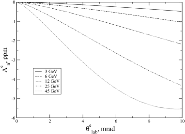
Figure 2: Beam SSNA as a function of the lab scattering angle for different beam energies: 3 GeV (solid line), 6 GeV (dashed line), 12 GeV (dash-dotted line), 25 GeV (dash-double-dotted line) and 45 GeV (dotted line).

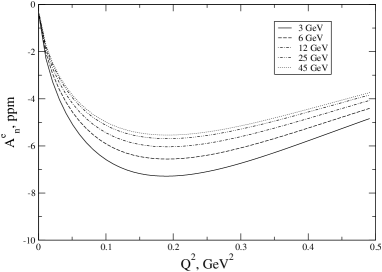
Figure 3: Beam SSNA as a function of $Q^{2}$ for different beam energies. Notation is as in Fig.2.

We also calculated the contribution of the elastic intermediate proton state to the beam SSNA for high energies and small electron scattering angles using the formalism of Ref.aam and found it to be highly supressed compared to the inelastic excitations. For the kinematics of SLAC E158 E158 , this supression is a few orders of magnitude due to different angular and energy behavior of these contributions.

Shown in Fig.3 are the calculations for beam SSNA as a function of $Q^{2}$ for different energies of incident electrons. One can see that at small $Q^{2}$, the asymmetry follows $\sqrt{Q^{2}}$ behavior desribed by Eq.(24), while at higher $Q^{2}$ the asymmetry turns over and starts to decrease due to the introduced exponential form factor $\exp{(-BQ^{2}/2)}$. It can be seen that at fixed $Q^{2}$ the magnitude of beam SSNA is predicted to be approximately constant, as follows from slow logarithmic energy dependence of the total photoproduction cross section.

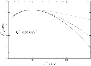
Figure 4: Beam SSNA as a function of c.m.s. energy for fixed Q² = 0.05 GeV² for different parameterizations of the total photoproduction cross section. See Fig.5 for notation.

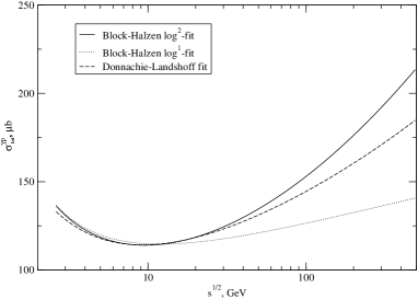
Figure 5: Different parameterizations of total photoproduction cross section at high energies used in the present calculation. A solid (dotted) line is a double-logarithmic fit 1 (single-logarithmic fit 3) from Block and Halzen block and a dashed line is an original Donnachie and Landshoff fit DL .

The latter feature is demonstrated in Fig.4, showing the calculated beam SSNA at fixed $Q^{2}$ in a wide energy range up to $\sqrt{s}$=500 GeV, where we used several parameterizations for the total photoproduction cross section on a proton from Refs.block ; DL , shown in Fig.5. The physical reason for the almost constant photoproduction cross sections at high energies is believed to be soft Pomeron exchange DL , therefore the beam SSNA in the considered kinematics is sensitive to the physics of soft diffraction.

The predicted $Q^{2}$ and energy dependence of beam SSNA, along with its relatively large magnitude, is quite different from the model expectations assuming that no hadronic intermediate states are excited in the TPE amplitude. Our unitarity-based model of small-angle electron scattering predicts the magnitude of the beam SSNA to reach a few ppm in a wide range of beam energies. The good news is that it makes beam SSNA measurable with presently reached fraction-of-ppm precision of parity-violating electron scattering experiments PViol . On the other hand, the experiments measuring parity-violating observables need to use special care to avoid possible systematic uncertainties due to the parity-conserving beam SSNA. Fortunately, these effects can be experimentally separated using different azimuthal dependences of these asymmetries.

In the present paper we calculate the beam SSNA for small values of $Q^{2}$ and provide physics arguments for the dominance of contributions from collinear photons in the TPE mechanism. For electron energies above the nucleon resonance region and small $Q^{2}$ the contribution of collinear virtual photons leads to the beam SSNA that is negative and has the order of $m_{e}\sqrt{Q^{2}}\sigma^{\gamma p}_{tot}$, where $\sigma^{\gamma p}_{tot}$ is the total photoproduction cross section on the proton. This quantity is multiplied by the factor of the order unity that includes a single-logarithm term. The fact that the beam SSNA does not decrease with the beam energy at fixed $Q^{2}$ makes it attractive for experimental studies at higher energies, for example, the energies to be reached at Jefferson Lab after the forthcoming 12-GeV upgrade of CEBAF.

References

- (1) N.F. Mott, Proc. R. Soc.London, Ser. A 135, 429 (1935).
- (2) A.O. Barut and C. Fronsdal, Phys. Rev. 120, 1871 (1960).
- (3) F. Guerin, C. A. Picketty, Nuovo Cim. 32, 971 (1964); J. Arafune, Y. Shimizu, Phys. Rev. D 1, 3094 (1970); U. Gűnther, R. Rodenberg, Nuovo Cim. A 2, 25 (1971); A. De Rujula, J.M. Kaplan and E. De Rafael, Nucl. Phys. B 35, 365 (1971); T.V. Kukhto et al., Preprint JINR–E2–92–556, Feb. 1993.
- (4) A.V. Afanasev, I.V. Akushevich, N.P. Merenkov, arXiv:hep-ph/0208260.
- (5) S.P. Wells et al., SAMPLE Collaboration, Phys. Rev. C 63, 064001 (2001).
- (6) M. Gorshtein, P.A.M. Guichon, M. Vanderhaeghen, arXiv:hep-ph/0404206.
- (7) Y.C. Chen, A.V. Afanasev, S.J. Brodsky, C.E. Carlson, and M. Vanderhaeghen, arXiv:hep-ph/0403058, to appear in Phys. Rev. Lett.
- (8) F. Maas et al., MAMI /A4 Collaboration, in preparation.
- (9) SLAC E158 Experiment, contact person K. Kumar.
- (10) G. Cates, K. Kumar, D. Lhuiller, spokespersons HAPPEX-2 Experiment, JLab E-99-115: D. Beck, spokesperson JLab/G0 Experiment, JLab E-00-006, E-01-116.
- (11) B. Pasquini and M. Vanderhaeghen, arXiv:hep-ph/0405303.
- (12) R. Tarrach, Nuovo Cim. A 28, 409 (1975).
- (13) B.L.Joffe, V.A. Khose, and L.N. Lipatov, Hard Processes, North Holland, Amsterdam (1984).
- (14) K. Hagiwara et al. [Particle Data Group Collaboration], Phys. Rev. D 66, 010001 (2002).
- (15) T. H. Bauer, R. D. Spital, D. R. Yennie and F. M. Pipkin, Rev. Mod. Phys. 50, 261 (1978) [Erratum-ibid. 51, 407 (1979)].
- (16) M. M. Block and F. Halzen, arXiv:hep-ph/0405174.
- (17) A. Donnachie and P. V. Landshoff, Phys. Lett. B 296, 227 (1992).