Prospects for Observing an Invisibly Decaying Higgs Boson in $t\bar{t}H$ Production at the LHC

Abstract

In this thesis we study the prospects for observing the invisibly decaying Higgs boson in the associated $t\bar{t}H$ production at the LHC. The results of the Monte Carlo simulations of signal and background processes show that there is a possibility of observing the statistically significant number of signal events required for the discovery. Moreover, the analysis can be further improved to reduce the number of false reconstructions of the $W$ boson.

The analysis of the $t\bar{t}H$ production is independent of the model in which the Higgs boson decays into the invisible channel. There are several possibilities for models where $H\to invisible$ can be of interest. For this thesis, we have studied the simplest supersymmetric model, called mSUGRA. The results of the scans of the mSUGRA model parameter space show that the regions, where the branching ratio of the lightest neutral Higgs boson to the lightest neutralino pair is high, are excluded by current experimental constraints. The $h\to b\bar{b}$ channel dominates, and the possibility for discovery in this channel will not be suppressed by the invisible decays. This result does not disqualify invisible channel as possible signature in other models.

Chapter 4 of this thesis is based on the published paper: B.P. Kersevan, M. Malawski, E. Richter-Wąs: Prospects for observing an invisibly decaying Higgs boson in the $t\bar{t}H$ production at the LHC, The European Physical Journal C - Particles and Fields, 2003, vol. 29, no. 4, pp. 541 - 548.

Chapter 1 Introduction

The Higgs boson is a very important element of the modern theory of elementary particles and their interactions, called the Standard Model. By means of spontaneous symmetry breaking the Higgs mechanism is used to introduce mass to other particles. The Higgs boson remains the last undiscovered particle predicted by the Standard Model. The most important large-scale experiments of these days, at the Large Hadron Collider at CERN and at Tevatron at Fermilab aim at the discovery of this particle.

Worldwide collaborations of scientists are studying the possible production and decay channels, where the Higgs boson may be observed. There are theories, in which the Higgs boson can decay into the invisible channel. This can occur when the Higgs decays into particles which interact very weakly with the matter, so they cannot be observed in the detector. There are various models that may lead to such invisible decays. These models include the decay into the lightest neutralinos in the supersymmetry models, or into neutrinos in the models of the neutrino mass generation, such as extra dimensions, TeV-scale gravity, Majorana models or 4th generation lepton [12].

The associated production of the Higgs boson and a $t\bar{t}$-quark pair can be an interesting channel leading to the observation of the invisible Higgs boson. The top quark production is a process with a very characteristic topology, so it can be used to effectively filter the events in which Higgs production takes place. One of the objectives of this thesis was to study the possibility of observing the Higgs boson in this channel using simulations the Atlas detector at LHC.

Supersymmetry (SUSY) is considered by many theorists as the most probable extension of the Standard Model. SUSY assumes a symmetry between fermions and bosons, introducing superpartners for each of the known elementary particles. The Minimal Supersymmetric extension of the Standard Model (MSSM) predicts the existence of the Lightest Supersymmetric Particle (LSP), which does not decay into normal particles and is a candidate for dark matter. A Higgs boson, decaying into a pair of LSPs, can give an invisible signature.

In order to obtain a more realistic estimation of the $t\bar{t}H$ process analysis results, it is necessary to discern the cross-section of the $t\bar{t}H$ production and the branching ratio of the Higgs to the invisible channel. SUSY models allow for such predictions. In this thesis, we describe the results of the scans of the mSUGRA model parameter space. The objectives of the scans were to find such regions in the parameter space, where the branching ratio of the Higgs into the invisible channel is large enough to make the results of the analysis statistically significant. The production process was studied only for the lightest Higgs boson in the so-called decoupling limit, i.e. in the region where its coupling to fermions and bosons is almost equal to that of the Standard Model Higgs boson of the same mass.

The thesis is organized as follows: Chapter 2 provides a theoretical introduction to the Standard Model Higgs boson and gives an overview of the current and planned experiments for Higgs boson discovery. Chapter 3 provides a brief introduction to supersymmetry and the specific mSUGRA model that can lead to an invisible Higgs decay. In Chapter 4 we describe the analysis of the $t\bar{t}H,H\to invisible$ process based on Monte Carlo simulations of the ATLAS detector at LHC. Chapter 5 presents the results of the scans of the mSUGRA model parameter space, where the invisible decay channel is possible. The conclusions are summarised in Chapter 6.

Chapter 2 The Higgs Boson

2.1 The Standard Model and the Higgs Theory

The Standard Model (SM for short), is currently regarded as a successful theory describing elementary particles and their interactions. SM is based on the quantum field theory. It assumes the existence of fermion fields representing matter and gauge fields that carry interactions. Matter is composed of three generations of quarks and leptons. For the spinor fields $\psi$, we have the Dirac Lagrangian:

$$L=\bar{\psi}(i\gamma^{\mu}\partial_{\mu}-m)\psi.$$ (2.1)

>From this Lagrangian we can derive the Dirac equation, which is the equation of motion of free relativistic particles and antiparticles (fermions). In order to introduce interactions into the model, we postulate the gauge invariance of the fields. The Lagrangian should be invariant under the $U(1)$ gauge transformation:

$$\psi\to e^{-i\alpha(x)}\psi.$$ (2.2)

For the Lagrangian (2.1) to be invariant, we need to introduce a new vector field $A_{\mu}$ and derive a new Lagrangian:

$$L_{D}=L-e\bar{\psi}\gamma^{\mu}A_{\mu}\psi,$$ (2.3)

where the transformation law for the $A_{\mu}$ vector field is:

$$A_{\mu}\to A^{\prime}_{\mu}=A_{\mu}+\frac{1}{e}\partial_{\mu}\alpha(x).$$ (2.4)

To the Lagrangian (2.3) we also add a term that yields the equations for gauge fields. For the electromagnetic field, the term is:

$$L_{A}=-\frac{1}{4}F_{\mu\nu}F^{\mu\nu},F_{\mu\nu}=\partial_{\mu}A_{\nu}-\partial_{\nu}A_{\mu}.$$ (2.5)

Such a Lagrangian can provide the Maxwell equations for electromagnetic fields and the Dirac equations for fermions:

$$\Box A^{\nu}=e\bar{\psi}\gamma^{\nu}\psi=j^{\nu};\quad\gamma^{\mu}(i\partial_{\mu}-eA_{\mu})\psi-m\psi=0.$$ (2.6)

In the case of a multiplet of $N$ particles, we have a more general Dirac Lagrangian:

$$L=\bar{\Psi}(i\gamma^{\mu}\partial_{\mu}-M)\Psi,$$ (2.7)

where $\Psi$ is an $N-$component vector. When we require the gauge invariance of such a theory, the transformation has the following form:

$$\Psi^{\prime}=G\Psi,$$ (2.8)

where $G$ is the $N\times N$ unitary matrix, $detG=1$. These matrices form the group $SU(N)$. The $SU(N)$ invariance requires the introduction of $N^{2}-1$ vector fields $G^{n}_{\mu}$ and modification of the Lagrangian:

$$L_{D}=L-g\bar{\Psi}\gamma^{\mu}\sum_{n}T^{n}G^{n}_{\mu}\Psi,$$ (2.9)

where $T^{n}$ are generators of the $SU(N)$ group. By introducing the operators:

$$\hat{G}_{\mu}=\sum_{n}G^{n}_{\mu}T^{n},\quad\hat{G}_{\mu\nu}=\partial_{\mu}\hat{G}_{\nu}-\partial_{\nu}\hat{G}_{\mu}+ig[\hat{G}_{\mu},\hat{G}_{\nu}],$$ (2.10)

we can construct the Lagrangian for the vector fields:

$$L_{G}=-\frac{1}{2}Tr(\hat{G}_{\mu\nu}\hat{G}^{\mu\nu})$$ (2.11)

The full Lagrangian of the $SU(N)$ theory has the following form:

$$L_{YM}=\bar{\Psi}(\gamma^{\mu}[i\partial_{\mu}-g\hat{G}_{\mu}]-M)\Psi-\frac{1}{2}Tr(\hat{G}_{\mu\nu}\hat{G}^{\mu\nu})$$ (2.12)

To describe the electroweak interactions for one generation of leptons or quarks, we need the $SU(2)_{L}\times U(1)$ group. The doublet $\Psi$ consists of the (lepton, neutrino) pair or (up-, down-)type quark pair respectively. The left-handed components $\Psi_{L}\equiv L$ of these spinors transform as the fundamental representation of the $SU(2)$ group, while the right-handed components $\Psi_{R}\equiv R$ are singlets with respect to this group. All members of the doublet transform under the $U(1)$ group. Consequently, we need four vector fields, $B_{\mu}$ corresponding to $U(1)$ and $B^{k}_{\mu},(k=1,...,3)$ for $SU(2)$. These fields give the fermion Lagrangian:

$$\begin{array}[]{lcl}L_{F}&=&i\bar{L}\gamma^{\mu}\partial_{\mu}L-\bar{L}\gamma^{\mu}(\frac{1}{2}g^{\prime}Y_{L}B_{\mu}+gB^{k}_{\mu}T^{k})L\\ &+&i\bar{\psi}^{1}_{R}\gamma^{\mu}\partial_{\mu}\psi^{1}_{R}-\bar{\psi}^{1}_{R}\gamma^{\mu}\frac{1}{2}g^{\prime}Y_{1R}B_{\mu}\psi^{1}_{R}\\ &+&i\bar{\psi}^{2}_{R}\gamma^{\mu}\partial_{\mu}\psi^{2}_{R}-\bar{\psi}^{2}_{R}\gamma^{\mu}\frac{1}{2}g^{\prime}Y_{2R}B_{\mu}\psi^{2}_{R}.\\ \end{array}$$ (2.13)

In this Lagrangian, the weak hypercharge is denoted by $Y$. The Lagrangian for vector fields has the following form:

$$L_{V}=-\frac{1}{4}B_{\mu\nu}B_{\mu\nu}-\frac{1}{4}\sum_{k}B^{k}_{\mu\nu}B^{k}_{\mu\nu}.$$ (2.14)

The fermion Lagrangian (2.13) cannot contain the mass term $\bar{\Psi}\Psi$ which is not invariant with respect to the $SU(2)$ group, since the left and right components transform differently, and:

$$\bar{\Psi}\Psi=\bar{\Psi}_{R}\Psi_{L}+\bar{\Psi}_{L}\Psi_{R}.$$ (2.15)

Moreover, $B^{k}_{\mu}$ fields are also massless, since we do not obtain the linear mass terms in motion equations from the Lagrangian (2.14)..

The model with all particles being massless is unsatisfactory, since we observe massive particles in the experiments. The solution to this problem is the Higgs mechanism. We add to our model one more $SU(2)$ doublet, consisting of two complex scalar fields:

$$H=\left[\begin{array}[]{c}h_{1}\\ h_{2}\end{array}\right],$$ (2.16)

called the Higgs field. The Lagrangian for these fields has to be gauge-invariant under $U(1)$ and $SU(2)$. We can choose such a gauge in which the Higgs field has the form:

$$H=\left[\begin{array}[]{c}0\\ h\end{array}\right],$$ (2.17)

where $h$ is the real function. This means that there is only one physical degree of freedom, so the Higgs field can give one neutral scalar particle. Very important in the construction of the Higgs Lagrangian is the substitution of the mass term by the Higgs potential. We postulate:

$$L_{H}=L_{H}^{free}-V=\partial_{\mu}H^{\dagger}\partial_{\mu}H-\mu^{2}H^{\dagger}H-\lambda[H^{\dagger}H]^{2}.$$ (2.18)

When $\mu^{2}<0$ the Higgs potential has a non-trivial minimum as shown in Fig. 2.1. The minimum is for:

$$H^{\dagger}H=-\frac{\mu^{2}}{2\lambda}.$$ (2.19)

We can choose the phase of the solution as:

Figure 2.1: Mexican-hat Higgs potential with a non-zero minimum

$$H=H_{0}=\left[\begin{array}[]{c}0\\ v/\sqrt{2}\end{array}\right];\quad v^{2}=-\frac{\mu^{2}}{\lambda}$$ (2.20)

Such a solution breaks the gauge symmetry. This is called the spontaneous symmetry breaking, since the potential itself is gauge-invariant, whereas the vacuum state breaks the symmetry. The Lagrangian containing interactions of the Higgs and the vector fields has the following form:

$$L=-\frac{1}{4}B_{\mu\nu}B_{\mu\nu}-\frac{1}{4}\sum_{k}B^{k}_{\mu\nu}B^{k}_{\mu\nu}+\frac{v^{2}}{8}((g^{\prime}B_{\mu}-gB^{3}_{\mu})+g^{2}(B^{1}_{\mu}B^{1}_{\mu}+B^{2}_{\mu}B^{2}_{\mu}))$$ (2.21)

This Lagrangian contains the terms bilinear in fields. We need to diagonalize this expression and derive mass coefficients. For components $B^{1}_{\mu}$ and $B^{2}_{\mu}$ the Lagrangian is already diagonal, so we obtain the mass terms:

$$M^{1}=M^{2}=\frac{gv}{2}$$ (2.22)

We can form combinations for particles with a definite charge:

$$W^{\pm}=\frac{B^{1}_{\mu}\pm B^{2}_{\mu}}{\sqrt{2}}.$$ (2.23)

These states form the charged $W$ bosons that carry the electroweak interactions. We also have combinations that yield the neutral bosons:

$$Z_{\mu}=\frac{-g^{\prime}B_{\mu}+gB^{3}_{\mu}}{\sqrt{g^{\prime 2}+g^{2}}}.$$ (2.24)

The mass of these bosons is:

$$M_{Z}=\frac{v\sqrt{g^{\prime 2}+g^{2}}}{2}$$ (2.25)

The remaining combination diagonalizing (2.21) is

$$A_{\mu}=\frac{g^{\prime}B_{\mu}+gB^{3}_{\mu}}{\sqrt{g^{\prime 2}+g^{2}}}.$$ (2.26)

This component is not present in the Lagrangian, so the mass coefficient must vanish. The massless field represents the photon. The ratio between the masses of $W$ and $Z$ bosons defines the Weinberg angle:

$$\frac{M_{W}}{M_{Z}}=\frac{g}{\sqrt{g^{\prime 2}+g^{2}}}\equiv\cos\theta_{W}.$$ (2.27)

To construct the Lagrangian for the Higgs field, we can rewrite it by distinguishing the vacuum part from the dynamical part:

$$H(x)=H_{0}+h(x),\quad h(x)\equiv\left[\begin{array}[]{c}0\\ h(x)\end{array}\right].$$ (2.28)

The Lagrangian for this field can be written in the form:

$$L_{H}=\partial_{\mu}h\partial^{\mu}h+2\mu^{2}h^{2}-2\sqrt{2}\lambda vh^{3}-\lambda h^{4}+\frac{g}{cos\theta_{W}}[vh+h^{2}][Z_{\mu}Z_{\mu}+2\cos\theta_{W}W^{+}_{\mu}W^{-}_{\mu}].$$ (2.29)

This Lagrangian gives the coupling of the Higgs field to the vector bosons and the Higgs mass:

$$m_{H}=-2\mu^{2}=2\lambda v.$$ (2.30)

This means that the value of the $v$ parameter is not enough to determine the Higgs mass, but it also depends on $\lambda$, which is a free parameter of the Standard Model.

The Higgs mechanism also gives mass to fermions. This is done by introducing the Yukawa couplings to the Lagrangian:

$$L_{Y}=-G_{1}[\bar{L}\tilde{H}\psi_{1R}+\bar{\psi}_{1R}\tilde{H}^{\dagger}L]-G_{2}[\bar{L}H\psi_{2R}+\bar{\psi}_{2R}H^{\dagger}L],$$ (2.31)

where

$$\tilde{H}=[h_{0}+h(x)]\left[\begin{array}[]{c}1\\ 0\end{array}\right].$$ (2.32)

For $h(x)\equiv 0$ we obtain

$$L_{Y}=-G_{1}h_{0}\bar{\psi}_{1}\psi_{1}-G_{2}h_{0}\bar{\psi}_{2}\psi_{2},$$ (2.33)

giving us the fermion masses:

$$m_{1}=G_{1}h_{0};\quad m_{2}=G_{2}h_{0}.$$ (2.34)

Similarly, we obtain the couplings of the Higgs field to fermions in the Lagrangian:

$$L_{Y}=-G_{1}h(x)\bar{\psi}_{1}\psi_{1}-G_{2}h(x)\bar{\psi}_{2}\psi_{2}.$$ (2.35)

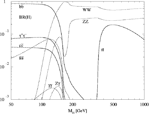
>From these equations we can see that the coupling of the Higgs boson to fermions is proportional to the fermion mass. As a consequence, we can predict that the Higgs boson will mostly decay into the heaviest lepton or quark pairs.

2.2 Current Experimental Results

The Standard Model predictions have passed all experimental tests conducted so far. The electroweak gauge bosons $W$ and $Z$ were detected at the LEP experiment at CERN and the $t$ quark was observed at the Tevatron. Only the Higgs boson remains as the last undiscovered elementary particle of the Standard Model. Discovery of the Higgs boson will enable verification of theoretical foundations of the Standard Model.

The possibilities of observing the Higgs particle both in $e^{+}e^{-}$ and in hadron colliders have been extensively analyzed. Since the coupling of the Higgs to other particles is proportional to their masses, the Higgs production and decay often involve the heavy quarks $t$ or $b$. Sample processes of Higgs production, such as Higgs-strahlung and weak boson fusion are shown in Fig 2.2.

Figure 2.2: Processes of Higgs production

The branching ratios of the Higgs boson to the others particles depend on the Higgs mass. Fig. 2.3 shows the branching ratios for various possible decay channels.

Figure 2.3: The branching ratios of the Standard Model Higgs boson [7].

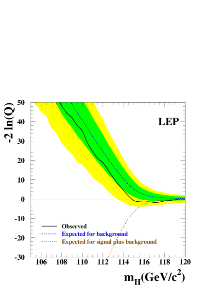
The results gathered at LEP from direct search for the Higgs boson and from the precision electroweak measurements provide some approximate limits to the Higgs boson mass. Direct search at LEP has excluded the existence of the Higgs boson with a mass $m_{H}<114.4$ GeV, at a 95% confidence level. The Fig 2.4 shows the expected and observed behavior of the statistic defined in [1].

Figure 2.4: The results of direct search for the SM Higgs boson at LEP [1].

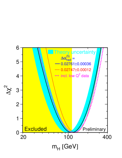
The precise measurements of the electroweak boson masses and couplings can also give an estimation of the Higgs boson mass. The combined results from the LEP and Tevatron experiments are shown in Fig. 2.5. They suggest the preferred Higgs boson mass to be: $m_{H}=113(+62-42)$ GeV at a 68% confidence level. They also set the upper limit to be about 237 GeV at a 95% confidence level.

Figure 2.5: The fit to electroweak measurements at LEP, setting bounds on the Higgs boson mass [16]

2.3 LHC Discovery Potential

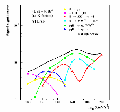
The LHC experiment will search for the SM Higgs boson in collisions of proton-proton pairs. The ATLAS and CMS experiments are preparing for possible discovery channels. Fig. 2.6 shows the ATLAS discovery potential for the SM Higgs boson for the integrated luminosity of 30 fb${}^{-}1$ [2]. It can be seen that the total estimated significance is higher than the $5\sigma$ discovery threshold for the Higgs mass range between 100 and 200 GeV.

Figure 2.6: ATLAS discovery potential for the SM Higgs boson [2]

Chapter 3 Supersymmetry

3.1 Introduction to Supersymmetric Theories

In spite of their success and compatibility with experimental results, both the Standard Model and the Higgs mechanism outlined in Chapter 2 remain unsatisfactory as theories [10]. One of the problems that the Standard Model does not solve is the hierarchy problem. This is a problem of the sensitivity of the Higgs mass to quantum corrections from the particles coupling to the Higgs boson. It so happens that the corrections from bosons and from fermions have opposite signs. Thus, the corrections would cancel each other out if each of the known fermions had a bosonic partner of the same mass and each boson had a fermionic partner. Such a symmetry is called supersymmetry [19].

Supersymmetry transforms boson states into fermions, and vice versa. This can be expressed as follows:

$$Q|Boson\rangle=|Fermion\rangle;\quad Q|Fermion\rangle=|Boson\rangle$$ (3.1)

The supersymmetry generator $Q$ is an anticommuting spinor that satisfies the following algebra:

$$\{Q,Q^{\dagger}\} = P^{\mu}$$ (3.2)

$$\{Q,Q\} = \{Q^{\dagger},Q^{\dagger}\}=0$$ (3.3)

$$\left[P^{\mu},Q\right] = \left[P^{\mu},Q^{\dagger}\right]=0$$ (3.4)

Supersymmetric particles can form multiplets, consisting of bosonic and fermionic states, called supermultiplets. All particles and their superpartners from the same supermultiplets have the same masses, since the $P^{2}$ operator commutes with the $Q,Q^{\dagger}$. The supersymmetry generators commute also with the generators of gauge transformations. Hence, particles in the same supermultiplet have the same electric charge, weak isospin and color degrees of freedom. In each supermultiplet, the number of fermionic degrees of freedom $n_{F}$ is equal to the number of bosonic degrees of freedom $n_{B}$:

$$n_{F}=n_{B}$$ (3.5)

The simplest possibility for a supermultiplet includes a single Weyl fermion with two helicity states and a complex scalar field with two degrees of freedom. Such a combination is called the chiral or matter supermultiplet. The next simplest possibility is the supermultiplet with a massless spin-1 vector boson, which has two degrees of freedom. Its superpartner is a massless spin-1/2 Weyl fermion. Such a combination is called the vector supermultiplet.

3.2 Minimal Supersymmetric Standard Model

The Standard Model particles and their superpartners are presented in Table 3.1. The table shows the states before the electroweak symmetry is broken, i.e. the $W$ and $B$ bosons correspond to $B^{k}_{\mu}$ and $B_{\mu}$ fields from Lagrangian (2.14) and their partners are called winos and binos. After breaking this symmetry, new states appear: zino $\tilde{Z}$ and photino $\tilde{\gamma}$. All these particles and their interactions form the Minimal Supersymmetric extension to the Standard Model (MSSM).

In Table 3.1 we can see two Higgs doublets: $H_{u},H_{d}$. In the Standard Model, one complex scalar Higgs doublet was enough (see eq. (2.16)). Now, however, two complex doublets are required to give mass to the particles.

Table 3.1: The Standard Model particles and their superpartners before electroweak symmetry breaking

Particle		Spin	Spartner		spin
quarks:	$u,d$	1/2	squarks:	$\tilde{u},\tilde{d}$	0
lepton:	$l$	1/2	sleptons:	$\tilde{l}$	0
Higgs:	$H_{u},H_{d}$	0	higgsino:	$\tilde{H}_{u},\tilde{H}_{d}$	1/2
gluon:	$g$	0	gluino:	$\tilde{g}$	1/2
W bosons:	$W$	0	winos:	$\tilde{W}$	1/2
B bosons:	$B$	0	binos:	$\tilde{B}$	1/2

The free Lagrangian of the supersymmetric model can be written in the following form:

$$L_{\mbox{free}}=-\partial^{\mu}\phi^{*i}\partial_{\mu}\phi_{i}-i\psi^{{\dagger}i}\bar{\sigma}^{\mu}\partial\mu\psi_{i}+F^{*i}F_{i},$$ (3.6)

where $\phi$ are the scalar fields, $\psi$ are the Weyl spinors from the supermultiplet and $F$ is the auxiliary scalar field, required to fill the remaining scalar degrees of freedom.

The interaction can be introduced into the theory by adding the Lagrangian

$$L_{\mbox{int}}=-\frac{1}{2}W^{ij}\psi_{i}\psi_{j}+W^{i}F_{i}+c.c.,$$ (3.7)

where $W^{ij}$ and $W^{i}$ are the functions of the bosonic fields $\phi_{i}$. These terms can be expressed using the superpotential $W$:

$$W=\frac{1}{2}M^{ij}\phi_{i}\phi_{j}+\frac{1}{6}y^{ijk}\phi_{i}\phi_{j}\phi_{k},$$ (3.8)

and relations:

$$W^{ij}=\frac{\delta^{2}}{\delta\phi_{i}\delta\phi_{j}}W;\quad W^{i}=\frac{\delta W}{\delta\phi_{i}},$$ (3.9)

where $M^{ij}$ is the mass matrix for the fermion fields, and $y^{ijk}$ is a Yukawa coupling between the two fermions $\psi_{i}\psi_{j}$ and the scalar $\phi_{k}$.

In the case of the MSSM, the superpotential has the form:

$$W_{\mbox{MSSM}}=\bar{u}y_{u}QH_{u}-\bar{d}y_{d}QH_{d}-\bar{e}y_{e}LH_{d}+\mu H_{u}H_{d}.$$ (3.10)

In this equation we use the superfield notation, i.e. $H_{u},H_{d},\bar{u}$, etc. denote the chiral supermultiplets, as in Tab. 3.1. The $\mu$ term corresponds to the Higgs mass in the Standard Model.

3.3 Models of Supersymmetry Breaking

The experimental results show that supersymmetry has to be broken, since no sparticles with masses equal to their Standard Model partners have been discovered. Despite the symmetry breaking, we would like to preserve the supersymmetric relations between superpartners in the high energy sector of the theory, in order to keep the solution to the hierarchy problem valid. Such an approach is called the soft supersymmetry breaking. This can be expressed by an effective Lagrangian of the MSSM:

$$\begin{array}[]{ccl}L^{MSSM}_{soft}&=&-\frac{1}{2}(M_{3}\tilde{g}\tilde{g}+M_{2}\tilde{W}\tilde{W}+M_{1}\tilde{B}\tilde{B})+c.c.\\ &-&(\tilde{\bar{u}}a_{u}\tilde{Q}H_{u}-\tilde{\bar{d}}a_{d}\tilde{Q}H_{d}-\tilde{\bar{e}}a_{e}\tilde{L}H_{d})+c.c.\\ &-&\tilde{Q}^{\dagger}m^{2}_{q}\tilde{Q}-\tilde{L}^{\dagger}m^{2}_{L}\tilde{L}-\tilde{\bar{u}}m^{2}_{\bar{u}}\tilde{\bar{u}}^{\dagger}-\tilde{\bar{d}}m^{2}_{\bar{d}}\tilde{\bar{d}}^{\dagger}-\tilde{\bar{e}}m^{2}_{\bar{e}}\tilde{\bar{e}}^{\dagger}\\ &-&m^{2}_{H_{u}}H^{*}_{u}H_{u}-m^{2}_{H_{d}}H^{*}_{d}H_{d}-bH_{u}H_{d}+c.c.).\end{array}$$ (3.11)

We can see that in eq. (3.11) we have the $M_{1},M_{2}$ and $M_{3}$ gaugino mass terms, $a_{u},a_{d},a_{e}$ are the matrices of Yukawa couplings, and the $m^{2}_{i}$ terms are mass matrices of fermion families. Together with the Higgs sector parameters, it is necessary to have 105 free parameters in the MSSM. The experimental results that restrict the flavor-changing neutral currents and CP violation suggest that the squark and slepton mass matrices should be diagonal. This organizing principle helps reduce the number of parameters.

Such universality can be achieved by assuming that, at high energy scale, there exists some simple Lagrangian in which there are only a few common mass and coupling parameters. After applying the renormalization group equations to the masses and couplings to compute their values in the electroweak scale, we can obtain the full spectrum of the MSSM parameters. Such unification of couplings is in agreement with the GUT theories, which predict unification at the mass scale of $10^{16}$GeV. Since the high-energy scale theory cannot be observed directly, it is called the hidden sector, while the MSSM is called the visible sector.

There is more than one model that can lead to such supersymmetry breaking. All these models can be divided with respect to the type of interaction between the hidden sector and the visible one. In gravity-mediated sypersymmetry breaking one assumes the supergravity Lagrangian in the hidden sector and the gravitational interactions lead to supersymmetry breaking. On the other hand, in the gauge-mediated supersymmetry breaking models, one assumes that there exist some additional chiral supermultiplets, called messengers, which couple to the fields of the hidden sector and also to the MSSM fermions through gauge interactions.

An especially interesting model, called mSUGRA, is the minimal version of gravity-mediated supersymmetry breaking models. It assumes unifications of all fermion masses into $m_{1/2}$, all boson masses into $m_{0}$, and one common coupling constant $A_{0}$. To complete the model, it is necessary to add the $\tan\beta$ and sign $\mu$ parameters describing the Higgs sector. Thus, there are only 5 parameters:

$$m_{0},m_{1/2},A_{0},\tan\beta,\mbox{sign}\mu,$$ (3.12)

that can give the full MSSM spectrum after applying renormalization group equations to the electroweak scale.

The mass spectrum of the MSSM is subject to the electroweak symmetry breaking, similar to that of the Standard Model, which leads to mixing of the states. In the Higgs sector, we have two complex scalar doublets $H_{u}=(H_{u}^{+},H_{u}^{0})$ and $H_{d}=(H_{d}^{0},H_{d}^{-})$. The Higgs potential has a minimum for non-zero $H_{u}^{0}=v_{u}$ and $H_{d}^{0}=v_{d}$, and the ratio between them is called $\tan\beta$:

$$\tan\beta\equiv v_{u}/v_{d}$$ (3.13)

When the electroweak symmetry is broken, the Higgs doublets mix with the gauge bosons, to give masses to the $W^{\pm}$ and $Z^{0}$ bosons. Thus, from the eight original degrees of freedom only five remain. They form the five scalar boson states: CP-odd neutral scalar $A^{0}$, two charged scalars $H^{+},H^{-}$, and two CP-even scalars $h^{0}$ and $H^{0}$. It can be shown that $h^{0}$ is the lightest among these Higgs bosons of the MSSM.

Electroweak symmetry breaking causes the mixing among the sparticles and produces new mass eigenstates. Neutral higgsinos $\tilde{H}^{0}_{u},\tilde{H}^{0}_{d}$ and neutral gauginos $\tilde{B},\tilde{W}^{0}$ produce four neutral states called neutralinos denoted $\chi^{0}_{i}$ In a similar way, the charged higgsinos and winos form four charged states, called charginos – two with positive and two with negative electric charges.

In the MSSM we can define a new multiplicative quantum number, called $R-$parity. It is defined as:

$$P_{R}=(-1)^{3(B-L)+2s},$$ (3.14)

where $B$ is the barion number, $L$ is the lepton number, and $s$ is the spin of the particle. The Standard Model particles and the Higgs bosons have even $R-$parity ($P_{R}=1$), while all sparticles have odd $R-$parity ($P_{R}=-1$). The conservation of the $R-$parity has important phenomenological consequences. It implies that the lightest supersymmetric particle (LSP) with $P_{R}=-1$, must be stable, and all sparticles must eventually decay into a state which contains an odd number of LSPs.

One of the best candidates for the LSP is the lightest neutralino $\chi^{0}_{1}$. Since it is electrically neutral and interacts only weakly with ordinary matter, it becomes a good candidate for dark matter required by cosmology. Also, in the collider experiments, particles decaying into neutral LSPs can give an invisible signature (missing energy) in the detector.

3.4 Experimental Signals for Supersymmetry

Although supersymmetry helps solve many theoretical and phenomenological problems beyond the Standard Model, there is still no experimental evidence that supersymmetry really exists. No sparticles have been discovered so far. The LEP and Tevatron experiments have only set limits to the masses of supersymmetric particles [11]. E.g. the lightest Higgs boson $h^{0}$ has been excluded in the mass range below 91.0 GeV.

Figure 3.1: LHC discovery potential for the MSSM Higgs bosons [11]

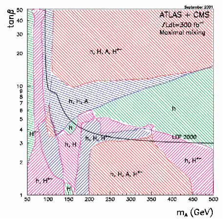
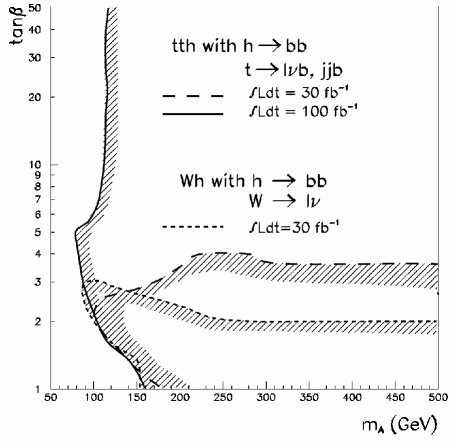
There are plans to search for supersymmetry at the LHC. Most of the sparticles with masses below 1TeV may be within reach of this collider. Fig. 3.1 shows the regions in the $(m_{A},\tan\beta)$ MSSM parameter space, where the various Higgs bosons can be observed. Most probable is the detection of the neutral $h$ boson, which is the lightest of the Higgs particles. Fig. 3.2 shows the regions, where $h$ can be observed in the $t\bar{t}h,h\to b\bar{b}$ channel. The possibility to observe the lightest Higgs boson in the invisible decay is studied in the following chapters of this thesis.

Figure 3.2: The $5\sigma$-discovery contour curves for the $t\bar{t}$ and $Wh$ with $h\to b\bar{b}$ channel in the $(m_{A},tan\beta)$ plane for the ATLAS experiment at luminosities of 30 fb^-1 [3].

Chapter 4 Analysis of $t\bar{t}H$ Production

4.1 Introduction

In this chapter we describe the analysis of the process that may allow us to observe the Higgs boson in the invisible channel. We describe the specific process and study possible backgrounds. In subsequent sections, we will provide details on the selection criteria that were applied to extract the interesting signal events from the background. The results and possible improvements are presented at the end of this chapter.

The possibilities to observe the Higgs boson in the invisible channel have been discussed throughout the past years. The prospects of detecting such a Higgs particle via its associated production with a gluon, $Z$ or $W$ bosons are described in [6]. The exploitation of associated $t\bar{t}$ production was suggested in [13]. The weak boson fusion process leading to the production of invisible Higgs is discussed in [9]. A more recent evaluation of the production with gauge bosons can be found in [12].

In this thesis we study the associated $t\bar{t}H$ production as suggested in [13]. The proposed approach was to require the leptonic decay of one of the $W$ bosons and the hadronic decay of the second one, as shown in Fig. 4.1. The final products are a single lepton, 2 $b$-jets and 2 jets from the hadronic decay of the $W$ boson. These jets and leptons can be identified by the detector so they can be used to trigger the filtering of interesting events. The evidence of the invisibly-decaying Higgs boson will be an excess of the selected events over the predicted background.

Figure 4.1: Process for observing the invisible Higgs.

4.2 Signal and Background Processes

In order to be able to observe such an excess of signal events, it is necessary to simulate and analyze the signal and possible backgrounds. The signal was simulated using the PYTHIA [21] Monte Carlo event generator. The generator simulated the proton–proton collisions at the LHC, at the 14 TeV center-of-mass energy.

$\mathbf{gg,q\bar{q}\to t\bar{t}H}$ :

This is the signal process generated using the PYTHIA event generator. The simulation is configured in such a way that 100% of the Higgs particles are decaying into the invisible channel, meaning they are not observed by the detector. The simulation assumes the Standard Model coupling of the Higgs to the $t$ quarks.

The background may come from processes which give a signature that is similar to the one generated by the signal process, i.e. an isolated lepton, 2 identified $b$-jets, 2 additional jets and missing transverse energy. The processes that may lead to such signatures, are the $t$-quark or $b$-quark production associated with the $W$- or $Z$-boson.

$\mathbf{gg,q\bar{q}\to t\bar{t}}$:

This is the main background process. It can yield the same signature as the signal, but the main difference is in the missing energy. In the case of the signal, it contains the energy of the invisible Higgs, while in the background it mostly carries the energy of the neutrino from the leptonic decay of the $W$ boson. Consequently, the missing energy will be the used to reduce this background.

$\mathbf{gg,q\bar{q}\to t\bar{t}Z,Z\to\nu\nu}$ :

This background can yield the same signature as the signal. The neutrinos coming from the $Z$ decay can carry significant missing energy, comparable with the signal.

$\mathbf{q\bar{q}\to t\bar{t}W,W\to\ell\nu}$ :

In this process, there can be 3 $W$ bosons: one from the associated production of the $t\bar{t}$ pair and 2 from the top-quarks decays. As a consequence, the results of the simulation where only the $W$-boson from the associated production is forced to decay into a lepton and the neutrino, should be finally multiplied by a combinatorial factor of 3. It assumes that the acceptance of the analysis is independent of the source of the lepton.

$\mathbf{gg,q\bar{q}\to b\bar{b}Z/\gamma^{*},Z/\gamma^{*}\to\ell\ell\oplus{\mathbf{\rm}jets}}$ :

This process can yield the same signature as the signal and its cross-section is several orders of magnitude larger. However, it is possible to reduce this background considerably by requiring the reconstruction of the top-quark from the hadronic jets. Also, requiring significant missing energy and vetoing additional leptons will suppress this background.

$\mathbf{q\bar{q}\to b\bar{b}W,W\to\ell\nu\oplus{\mathbf{\rm}jets}}$ :

This background can be suppressed by requiring the reconstruction of the top quark in the hadronic mode and significant transverse energy.

4.3 Event Generation and Detector Simulation

For the $t\bar{t}$ process event generation, the PYTHIA [21] and HERWIG [18] Monte Carlo generators were used. Additionally, the AcerMC [15] event generator was used to simulate other backgrounds. For these generators the initial parameters were set to default values.

For detector simulation, the ATLFAST [20] program was used. It implements a simplified simulation of the ATLAS detector at the LHC. The generated events serve as input to this program and it produces the detector response as output. It provides such observables as the 4-momenta of isolated leptons, jets, tagged $b$-jets and transverse energy. It is also possible to evaluate the missing transverse energy by integrating the total energy of particles detected and subtracting from the initial energy of colliding protons.

The simulation assumes 90% efficiency in lepton identification, 80% for jet reconstruction and 60% for $b$-jet identification (tagging). These efficiencies were taken into account while calculating the normalized number of events.

4.4 Analysis

The objective of the analysis is to apply such filters to the simulated processes that will suppress, as much as possible, the background while preserving a high number of signal events. The following filters are applied to the events:

Figure 4.2: Reconstructed mass of the top quark for the ttH events (number of events not normalized).

1. One isolated lepton is required. The lepton comes from semi-leptonic decay of one top quark. Events with more leptons are rejected in order to eliminate events coming from the $b\bar{b}Z/\gamma^{*}$ background.

2. Two identified (tagged) $b$-jets are required.

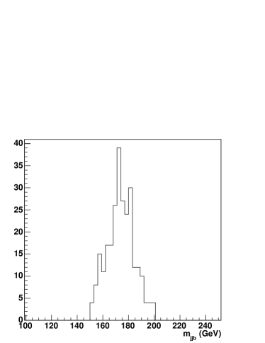
3. One top quark is required to be reconstructed from the hadronic decay mode $t\to jjb$. First, only such $jj$ pairs are selected from all possible combinations of jets, where $m_{jj}=m_{W}\pm$ 15 GeV. Additionally, only central jets with pseudo-rapidity $|\eta^{jet}|<2.0$ are allowed to reduce the number of events with jets coming from initial- or final-state QCD radiation instead of the $W$-boson decay. Next, the masses of all combinations of the selected $jj$ pairs and $b$-jets are calculated. The four-momenta of the jets are recalibrated so that the $m_{jj}$ gives $m_{W}$ exactly. The best combination of the $jjb$ system is chosen and the top quark is considered reconstructed if $m_{jjb}=m_{t}\pm 25$ GeV (see Fig. 4.2).

4. It is not possible to reconstruct the second top-quark which decays in the leptonic channel. This would require precise information on the missing energy, which in the case of the $t\bar{t}H$ events comes both from the leptonic decay of the top-quark and from the invisible Higgs. Instead, it is possible to use the transverse mass of the lepton end $\not E_{T}$  system to distinguish between the signal and the $t\bar{t}$ background, where

   $$m_{T}(\ell,\mbox{$\not E_{T}$})=\sqrt{2E_{T}^{\ell}\mbox{$\not E_{T}$}(1-cos\phi)}$$ (4.1)

   The Fig. 4.3 shows the distribution of $m_{T}(\ell,\mbox{$\not E_{T}$})$ for signal and background processes. It can be seen that for the $t\bar{t}$ process, where the missing energy comes from the leptonic decay of the $W$-boson, there is a sharp end of the distribution around the $W$ mass. To cut the big fraction of the $t\bar{t}$ events we require that $m_{T}(\ell,\mbox{$\not E_{T}$})>120$ GeV.

5. In addition to the $m_{T}(\ell,\mbox{$\not E_{T}$})$ cut, we also require a large missing transverse energy of the event: $\mbox{$\not E_{T}$}>150$ GeV.

6. The signal-to-background ratio is enhanced by the additional requirement of large transverse momenta in the reconstructed system, $\sum p_{T}^{\mathrm{rec}}>250$ GeV. The $\sum p_{T}^{\mathrm{rec}}=\sum p_{T}^{j}+p_{T}^{l}$ where the sum runs over the transverse momenta of reconstructed objects from top-quark decays: two $b$-jets, two light jets used for the reconstruction of the $W\to q\bar{q}$ decay and an isolated lepton. This further suppresses the background where true top quarks are not present, like $b\bar{b}Z$ and $b\bar{b}W$.

7. Finally, further enhancement of the signal-to-background ratio can be achieved by the additional requirement regarding cone separation, $R_{jj}$, between jets used for the $W\to jj$ reconstruction, the $R_{jj}<2.2$.

   $$R_{jj}=\sqrt{(\Delta\eta)^{2}+(\Delta\phi)^{2}}$$ (4.2)

   is a distance in the $(\eta,\phi)$ plane between the jets.

Figure 4.3: Reconstructed transverse mass of the lepton and $\not E_{T}$  system in the $t\bar{t}H$ events (left plot) and in the $t\bar{t}$ events (right plot). The dashed line denotes the distributions calculated from the true invisible energy of the primary products of W boson decays in these events, obtained by using the generator level information. The distributions are normalized to the number of events expected for an integrated luminosity of $30fb^{-1}$.

Table 4.1 shows the cumulative acceptance of the specified filters applied to selected processes.

Table 4.1: The cumulative acceptances for the specified selection criteria. Efficiencies for b-tagging and lepton identification are included. A Higgs boson mass of 120 GeV is assumed for signal events. Only the dominant background sources are listed.

Process	$t\bar{t}H$	$t\bar{t}Z$	$t\bar{t}$	$t\bar{t}$
	PYTHIA	AcerMC	PYTHIA	HERWIG
Trigger lepton	22%	22%	22%	22%
2 b-jets + 2 jets	5.0%	4.8%	4.9%	5.2%
rec. t-quark (jjb)	2.6%	2.4%	2.4%	2.6%
$m_{T}^{\ell,\mbox{$\not E_{T}$}}>120$ GeV	0.87%	0.93%	$4.1\cdot 10^{-4}$	$5.2\cdot 10^{-4}$
$\mbox{$\not E_{T}$}>150$ GeV	0.41%	0.53%	$2.3\cdot 10^{-5}$	$3.7\cdot 10^{-5}$
$\sum p_{T}^{\mathrm{rec}}>250$ GeV	0.40%	0.51%	$2.0\cdot 10^{-5}$	$3.2\cdot 10^{-5}$
$R_{\mathrm{jj}}<2.2$	0.28%	0.35%	$7.5\cdot 10^{-6}$	$1.2\cdot 10^{-5}$

We can see that the acceptance of signal events is about 0.3%, while the background is reduced by a factor of $10^{-}5-10^{-}6$.

After performing such selections, one can see that about 70% of the $t\bar{t}$ events come from the lepton-tau decay and 20% from the lepton-lepton decay of the top-quark pair in the PYTHIA sample with compatible fractions also found in HERWIG events. The lepton-tau label denotes one top quark decaying $t\to Wb\to\ell\nu b$ and another $t\to Wb\to\tau\nu b$, where $\ell$ stands for electron or muon. The lepton-lepton decay labels events with both top quarks decaying $t\to Wb\to\ell\nu b$. Finally, the lepton-hadron decay labels events with one top quark decaying $t\to Wb\to\ell\nu b$ and another $t\to Wb\to q\bar{q}b$.

In the cases of lepton-lepton and lepton-tau decays, the $jjb$ combination is thus made not from the true $W\to q\bar{q}$ decays, but from other jets coming from the initial- or final-state radiation (ISR/FSR). These events could hopefully be suppressed further by implementing a tau-jet veto and with more stringent requirements in the $t\to jjb$ reconstruction. The signal events, in contrast, contain only a $\sim 10\%$ fraction of lepton-tau and lepton-lepton decays. The relative fractions of signal and $t\bar{t}$ background events are shown in Figure 4.4.

Considering the relative fractions of the tau-lepton events in the signal and background, one can assume that the inter-jet cone separation, $R_{\mathrm{jj}}$, might provide some additional separation power; the $R_{\mathrm{jj}}$ for signal and $t\bar{t}$ background events are given in Figure 4.4. Subsequently, a loose cut of $R_{\mathrm{jj}}<2.2$ was applied; the final efficiencies are listed in Table 4.1.

Figure 4.4: The relative fractions of the $t\bar{t}$ decay modes are listed for signal and $t\bar{t}$ background simulated with PYTHIA (left plot). The $R_{\mathrm{jj}}$ cone separation between jets used in the $W\to jj$ reconstruction; the distributions are normalized to the number of events expected for an integrated luminosity of $30fb^{-1}$ (right plot).

Table 4.2: Expected numbers of events for an integrated luminosity of $30fb^{-1}$ and selection as specified in Table 4.1. Efficiencies for b-tagging and lepton identification are included. The (PY) and (HW) denote the results for the $t\bar{t}$ events generated with PYTHIA and HERWIG respectively. Also shown is the separate contribution to the $t\bar{t}$ background from the lepton-hadron events.

Process	No. of events
$t\bar{t}H$,
$m_{H}=100$ GeV	60
$m_{H}=120$ GeV	45
$m_{H}=140$ GeV	30
$m_{H}=160$ GeV	25
$m_{H}=200$ GeV	15
$t\bar{t}Z$	20
$t\bar{t}W$	20
$t\bar{t}$ (all)	115 (PY) , 190 (HW)
(only lepton-hadron)	15 (PY) , 30 (HW)
$b\bar{b}W$	5
$b\bar{b}Z/\gamma^{*}$	5

The expected numbers of events for an integrated luminosity of $30fb^{-1}$ are given in Table 4.2. Several values of the Higgs boson masses are studied, while assuming the Standard Model production cross-sections. The branching ratio of the Higgs boson to the invisible channel is assumed to be 100% in this analysis.

It can be seen that for the process $t\bar{t}$ generated with PYTHIA, the signal-to-background ratio is about 39% for a Higgs boson mass of 100 GeV and about 9% for a Higgs mass of 200 GeV. Of course, if only true reconstructed top-quark decays were allowed, these ratios would increase considerably.

It would also be possible to increase the signal-to-background ratio by setting more tight cuts on such observables as $R_{\mathrm{jj}}$, $\not E_{T}$, $\sum p_{T}^{\mathrm{rec}}$. However, such optimizations are not suitable at this moment, since they could lead to over-fitting to the results obtained by the particular implementations of the processes in event generators. It is clear that further optimization of the analysis should lead to an increase in the efficiency of rejecting "fake" $W\to jj$ reconstructions and eliminating the contribution of events with lepton-tau and lepton-lepton decays.

The basic measure of the quality of the analysis is the significance $S=s/\sqrt{b}$, where $s$ and $b$ are the numbers of signal and background events respectively. $S=5$ is assumed to be the discovery level, while $S=3$ is called the evidence level. $S=1.96$ corresponds to the 95% confidence level. We can define the $\xi^{2}$ parameter as:

$$\xi^{2}=\frac{\sigma{\rm(t\bar{t}H)}}{\sigma{\rm(t\bar{t}H)}_{\rm SM}}\times{\rm Br(H\to inv)}.$$

It can be used to estimate the minimal branching ratio required for the significance to reach the desired thresholds.

Taking the values from Table 4.2 we get $s=60$ for the $t\bar{t}H$ signal with $m_{H}=100GeV$ and $b=65$ for the total background that includes the (lep-had) $t\bar{t}$ events generated with PYTHIA. This yields $S=7.44$ and requires $\xi^{2}$ to be 0.67 and 0.4 for the discovery and evidence levels respectively. The values for the $t\bar{t}$ background and also for (lep-had) events are shown in Table 4.3.

Table 4.3: Estimated significance $S=s/\sqrt{b}$ for $t\bar{t}$ background and estimated branching ratios required for significance to reach the values of 5, 3 and 1.96

	all $t\bar{t}$				lep-had $t\bar{t}$
$m_{H}$	$s/\sqrt{b}$,	$\xi^{2}(5)$	$\xi^{2}(3)$	$\xi^{2}(1.96)$	$s/\sqrt{b}$	$\xi^{2}(5)$	$\xi^{2}(3)$	$\xi^{2}(1.96)$
100 GeV	4.67	1.07	0.64	0.42	7.44	0.67	0.4	0.26
120 GeV	3.5	1.43	0.86	0.56	5.58	0.9	0.54	0.35
140 GeV	2.34	2.14	1.28	0.84	3.72	1.34	0.81	0.53
160 GeV	1.95	2.57	1.54	1.01	3.1	1.61	0.97	0.63
200 GeV	1.17	4.28	2.57	1.68	1.86	2.69	1.61	1.05

Chapter 5 Scans of mSUGRA Model

5.1 Objective of the scans

The supersymmetric models as described in Chapter 3 allow a decay of the Higgs boson into a pair of the lightest neutralinos $\chi^{0}_{1}\chi^{0}_{1}$. This is an invisible channel when the neutralino is the LSP, which means it does not decay, but leaves the detector, leaving its signature only as missing energy. It is interesting to study for which parameters of the supersymmetric models, like mSUGRA, such decay is allowed and can lead to possible Higgs discovery. Results of such scans can be combined with results from similar scans for Higgs decaying into visible Standard Model particles.

In this thesis, the Suspect and HDECAY [8, 7] programs were used to perform the scan of the mSUGRA model parameter space. The goal of the scan was to identify the regions with high Higgs branching ratio to $\chi^{0}_{1}\chi^{0}_{1}$ pair. The analysis of the associated $t\bar{t}H$ production presented in [14] and discussed in Chapter 4 was performed with the assumption that the $BR(H\rightarrow\chi^{0}_{1}\chi^{0}_{1})$ was 100%. Therefore, it is necessary to multiply the results of the analysis by the branching ratio obtained from the scans. The estimates for minimal branching ratios required for the discovery or evidence signatures respectively are included in Table 4.3. In the scans, we will search for such areas in the parameter space, where the $BR(H\to\chi^{0}_{1}\chi^{0}_{1})$ can reach these values.

It is also interesting to check the branching ratio of Higgs to the $b\bar{b}$ pair. This decay is considered as the main channel where the Higgs can be observed in the same production mode. If the decay of $H\to\chi^{0}_{1}\chi^{0}_{1}$ is open, the $H\to bb$ will become suppressed. We can compare the branching ratio to the $b\bar{b}$ and the invisible channels and examine if the invisible decay should be considered as complementary for the observation.

5.2 Implementation of the Scans

For the scans, we have combined two programs. Suspect [8] takes as input the 5 parameters of the mSUGRA model (see eq. (3.12))and returns the spectrum of masses of MSSM particles. These parameters serve as input to the HDECAY [7] program, which computes the branching ratios of the Higgs to both Standard Model and MSSM particles.

The input parameters were selected to cover the most interesting regions of the mSUGRA space. The masses $m_{0}$ and $m_{1/2}$ were covered in the range of 0 to 500 GeV, with steps of 10 GeV. The $\tan\beta$ had values of 50, 25 and 12.5, …Three values of the $A_{0}$ parameter were chosen: -200, 0, 200 and both values of sign $\mu$ were used.

As the input for the Suspect and HDECAY programs, default parameters were used. For the drawing of plots, the ROOT framework was used [4].

5.3 Constraints on the Parameter Space

It is important to note that not all regions of the mSUGRA parameter space are allowed. First, it is possible that the mass of the stau is lower than that of the lightest neutralino. This would imply that the neutralino is not the LSP, contradicting the assumption that SUSY particles decay into the invisible channel. Such regions should be theoretically excluded.

Second, current experimental results from the LEP and Tevatron experiments, as well as from cosmological observations have excluded the existence of SUSY particles below certain mass limits. Such limits for the SUSY Higgs boson obtained by four combined LEP experiments is now set at 91.0 GeV [17]. More limits on the masses of other sparticles can be found in [11]. The constraints applied to the scans are shown in Table 5.1.

Additionally, the programs that were used for the scans have limitations related to numerical stability. Although several tests are performed internally by these programs, there are also points of the parameter space, where the calculations do not converge. Such points are also excluded from the scans.

Table 5.1: Experimental constraints on masses of sparticles used in the scan

Particle	Mass constraint
$h$	> 91.0 GeV
sleptons	> 80.0 GeV
chargino	> 103.6 GeV
gluino	> 195.0 GeV
neutralino	> 45.6 GeV

5.4 Results of the Scans

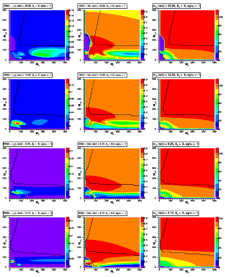
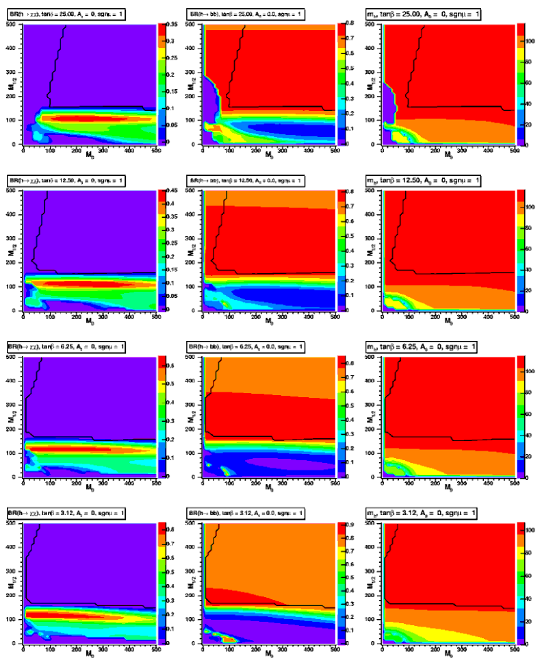
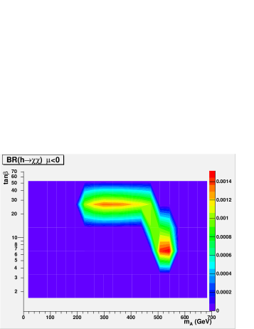
The resulting plots showing the contours of branching ratios are presented in Figs. 5.1-5.2. We selected the following values of tan$\beta$: 25, 12.5, 6.25, 3.12; both signs of $\mu$ and produced plots in the $(m_{0},m_{1/2})$ plane. We show only values of $A_{0}=0$, since other tested values (-200, 200) provide similar results. For $\tan\beta>25$ and $<3$ we observed more instability in the combined programs.

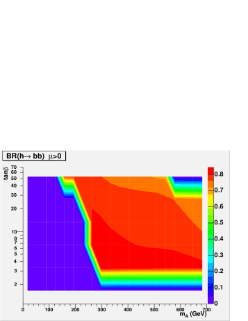
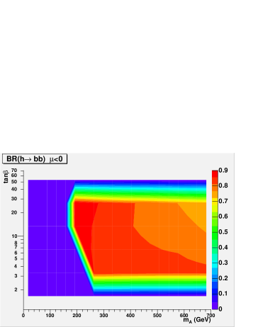
For each value of $\tan\beta$ and sign $\mu$ we show three contour plots in the $(m_{0},m_{1/2})$ plane: branching ratio of lightest Higgs boson to neutralinos, to the $b\bar{b}$ pair and the Higgs mass $m_{h}$. The theoretical and experimental constraints are indicated by the solid line: regions below and to the left of this line are excluded.

We can see that there are small regions where the $BR(h\to\chi^{0}_{1}\chi^{0}_{1})$ is dominant. For the $\mu>0$ and for small $\tan\beta$, the value of the BR can reach 0.9 for small regions of the parameter space. This would mean that assuming the possibility of analysis as described in Chapter 4 a sufficient excess of signal events would be observed to enable observation of the Higgs in the invisible channel. However, taking into account the experimental limits, it is very likely that the regions where the $BR(h\to\chi^{0}_{1}\chi^{0}_{1})$ is large, are excluded by current observations. On the other hand, the plots show that the branching ratio to $b$-quark is dominant in most of the regions that are not excluded. That confirms the need for the search for Higgs in this decay channel.

Figure 5.1: Scans of mSUGRA parameter space for $\mu<0$.

Figure 5.2: Scans of mSUGRA parameter space for $\mu>0$.

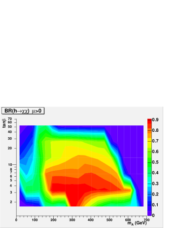
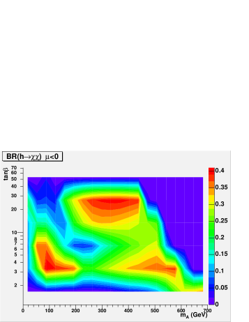
Figs. 5.3– 5.5 show the projection of the mSUGRA model onto the $(m_{A},tan\beta)$ plane. In the mSUGRA model the $m_{A}$ is not given explicitly as an independent variable, but is a function of the initial parameters. It means that one point from the $(m_{A},tan\beta)$ plane may correspond to more than one $(m_{0},m_{1/2})$ pair of initial parameters. In such a case, when plotting the values of branching ratios, we chose the maximum from these values.

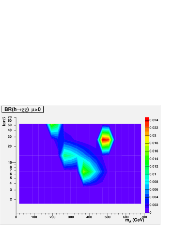
Fig. 5.3 shows the branching ratio $BR(h\to\chi^{0}_{1}\chi^{0}_{1})$ in a mSUGRA model without any theoretical and experimental constraints. We can see that there are regions where the $\chi^{0}_{1}\chi^{0}_{1}$ channel can be dominating. However, when we apply the constraints according to Table 5.1, we can see in Fig. 5.4 that all points with a high branching ratio are excluded, which is also seen in the $(m_{0},m_{1/2})$ plane. On the other hand, the $BR(h\to b\bar{b})$ can be very high even with constraints applied (Fig. 5.5).

Figure 5.3: $BR(h\to\chi^{0}_{1}\chi^{0}_{1})$ in mSUGRA model in the $(m_{A},tan\beta)$ plane, $A_{0}=0$, without applying any constraints.

Figure 5.4: The maximal values of $BR(h\to\chi^{0}_{1}\chi^{0}_{1})$ in mSUGRA models projected on the $(m_{A},tan\beta)$ plane, $A_{0}=0$, after applying theoretical and experimental constraints.

Figure 5.5: The maximum values of $BR(h\to bb)$ in mSUGRA models projected on the $(m_{A},tan\beta)$ plane, $A_{0}=0$, after applying theoretical and experimental constraints.

Chapter 6 Conclusions

In this thesis we studied the prospects for observing the invisibly decaying Higgs boson in the associated $t\bar{t}H$ production at the LHC. The results of Monte Carlo simulations of the signal and background processes have shown that there is a possibility of observing a statistically-significant number of signal events required for the discovery. Moreover, the analysis can still be improved to reduce the number of false reconstructions of the $W$ boson.

It is important to note that the analysis of the $t\bar{t}H$ production described in Chapter 4 is independent of the model in which the Higgs boson decays into the invisible channel. There are several possibilities for models where $H\to invisible$ can be of interest. These models include the decay into lightest neutralinos in the supersymmetry models, or decays into neutrinos in the various models of the neutrino mass generation, such as extra dimensions, TeV scale gravity, Majorana models or 4th generation lepton.

For this thesis we have studied only the simplest supersymmetric model, called mSUGRA. The results of the scans of the mSUGRA model parameter space show that the regions where the branching ratio of the Higgs particle to the lightest neutralino pair is high, are excluded by current experimental constraints. The $h\to b\bar{b}$ channel dominates and the prospects for discovery in this channel will not be suppressed by opening of invisible decay. This is very encouraging conclusion: we will much prefer to have Higgs boson discovered in the visible channel.

In less constrained SUSY models this however might not be the case. It would be also interesting to investigate other models that can lead to such a signature, not just the supersymmetric ones. This is out of the scope of this thesis, but might provide an interesting research subject.

Bibliography

- [1] ALEPH, DELPHI, L3 and OPAL Collaborations, The LEP Working Group for Higgs Boson Searches: Search for the Standard Model Higgs Boson at LEP, Phys. Lett. B 565 (2003) 61.
- [2] Asai, S. et al.: Prospects for the Search for a Standard Model Higgs Boson in ATLAS using Vector Boson Fusion, ATLAS note ATL-PHYS-2003-005.
- [3] ATLAS Collaboration: ATLAS Detector and Physics Performance - Technical Design Report, CERN/LHCC 99-14, 1999.
- [4] Brun, R., Rademakers, F.: ROOT - An Object Oriented Data Analysis Framework, Proceedings AIHENP’96 Workshop, Lausanne, Sep. 1996, Nucl. Inst. & Meth. in Phys. Res. A 389 (1997) 81-86. See also http://root.cern.ch/.
- [5] Cavalli, D. et al., The Higgs WG summary report from Les Houches 2001 Workshop, hep-ph/0203056.
- [6] Choudhury, D., Roy, D.P.: Signatures of an invisibly decaying Higgs particle at LHC, Phys. Lett. B322 (1994) 368.
- [7] Djouadi, A., Kalinowski, J., Spira, M.: “HDECAY: A program for Higgs boson decays in the standard model and its supersymmetric extension,” Comput. Phys. Commun. 108 (1998) 56, hep-ph/9704448.
- [8] Djouadi, A., Kneur, J.-L., Moultaka, G.: The program SUSPECT for the calculation of the SUSY Spectrum, version 2.102, hep-ph/0211331.
- [9] Eboli, O.J.P., Zeppenfeld, D.: Observing an invisible Higgs boson, Phys. Lett. B495 (2000) 147.
- [10] Ellis, J.: Beyond the Standard Model for Hillwalkers, hep-ph/9812235.
- [11] Gianotti, F. “Searches For Supersymmetry At High-Energy Colliders: The Past, The Present And The Future,” New J. Phys. 4 (2002) 63.
- [12] Godbole, R.M. et al., Search for ‘invisible’ Higgs signals at LHC via Associated Production with Gauge Bosons. hep-ph/0304137.
- [13] Gunion, J.F.: Detecting an Invisibly Decaying Higs Boson at a Hadron Supercollider, Phys. Rev. Lett. 72 (1994) 199.
- [14] Kersevan, B.P., Malawski, M., Richter-Wąs, E. Prospects for observing an invisibly decaying Higgs boson in the ttH production at the LHC, The European Physical Journal C - Particles and Fields, 2003, vol. 29, no. 4, pp. 541 - 548.
- [15] Kersevan, B.P., Richter-Wąs, E.: The Monte Carlo event generator AcerMC version 1.0 with interfaces to PYTHIA 6.2 and HERWIG 6.3, Comp. Phys. Commun. 149 (2003) 142.
- [16] The LEP Collaborations: ALEPH, DELPHI, L4, OPAL, the LEP Electroweak Working Group, the SLD Electroweak Working Groups: A Combination of Preliminary Electroweak Measurements and Constraints on the Standard Model, CERN 2003, hep-ex/0312023.
- [17] LEP Higgs Working Group Collaboration: Searches for the Neutral Higgs Bosons of the MSSM: Preliminary Combined Results Using LEP Data Collected at Energies up to 209 GeV. hep-ex/0107030.
- [18] Marchesini, G. et al.: HERWIG 6.5, Comp. Phys. Commun. 67 (1992) 465, Corcella, G. et al., JHEP 0101 (2001) 010.
- [19] Martin, S.P.: A Supersymmetry Primer, hep-ph/9709356.
- [20] Richter-Wąs, E., Froidevaux, D., Poggioli, L.: ATLFAST-2.0 a fast simulation package for ATLAS, ATLAS Internal Note ATL-PHYS-98-131 (1998).
- [21] Sjöstrand, T., Edén, P., Friberg, C., Lönnblad, L., Miu, G., Mrenna, S. an d Norrbin, E.: High Energy-Physics Event Generation with PYTHIA 6.1, Computer Phys. Commun. 135 (2001) 238.