Abstract

We analyze the indirect detection of neutralino dark matter in supergravity scenarios with non-universal soft scalar and gaugino masses. In particular, the gamma-ray flux arising from the galactic center due to neutralino annihilation is computed. In important regions of the parameter space it can be increased significantly (about two orders of magnitude) with respect to the universal scenario. This result is compared with the sensitivity of current and planned experiments, such as the satellite-based detectors EGRET and GLAST and the ground-based atmospheric telescope HESS. For example, for $\tan\beta<35$ the sensitivity region of GLAST and HESS can only be reached in non-universal scenarios.

1 Introduction

There are substantial evidences suggesting the existence of dark matter in the Universe. In addition to the observations of galactic rotation curves [1], cluster of galaxies, and large scale flows [2], implying $0.1\raise 1.29167pt\hbox{$\;<$\kern-7.5pt\raise-4.73611pt\hbox{$\sim\;$}}\Omega_{DM}h^{2}\raise 1.29167pt\hbox{$\;<$\kern-7.5pt\raise-4.73611pt\hbox{$\sim\;$}}0.3$, the recent data obtained by the WMAP satellite [3] confirm that dark matter must be present with $0.094\raise 1.29167pt\hbox{$\;<$\kern-7.5pt\raise-4.73611pt\hbox{$\sim\;$}}\Omega_{DM}h^{2}\raise 1.29167pt\hbox{$\;<$\kern-7.5pt\raise-4.73611pt\hbox{$\sim\;$}}0.129$.

The lightest neutralino, $\tilde{\chi}^{0}_{1}$, a particle predicted by the supersymmetric (SUSY) extension of the standard model, is one of the leading candidates for dark matter. It is specially interesting because, in addition to be usually stable, it is a weakly interacting massive particle (WIMP), and therefore it can be present in the right amount to explain the observed matter density.

There are promising methods for the indirect detection of WIMPs through the analysis of their annihilation products [4]. One of them consists of detecting the gamma rays produced by these annihilations in the galactic halo [5]-[24]. For this one uses atmospheric Cherenkov telescopes or space-based gamma-ray detectors. In fact, one of the space-based experiments, the Energetic Gamma-Ray Experiment Telescope (EGRET) on the Compton Gamma-Ray Observatory detected a signal [25] that apparently cannot be explained with the usual gamma-ray background. In particular, after five years of mapping the gamma-ray sky up to an energy of about 20 GeV, there are evidences of a source of gamma rays above about 1 GeV in the galactic center region with a value for the flux of about $10^{-8}$ cm^-2 s^-1. It is worth noticing, however, that alternative explanations for this result have been proposed modifying conveniently the standard theory of galactic gamma ray [26].

Projected experiments might clarify the situation. For example, a larger sensitivity will be provided by the Gamma-ray Large Area Space Telescope (GLAST) [27], which is scheduled for launch in 2006. In addition, energies as high as 300 GeV can be measured testing models with heavy dark matter more easily than EGRET. Even if alternative explanations solve the data problem pointed out by EGRET, GLAST will be able to detect a smaller flux of gamma rays from dark matter $\sim 10^{-10}$ cm^-2 s^-1. Besides, ground-based atmospheric Cherenkov telescopes are complementary to space-based detectors. In particular, the High Energy Stereoscopic System (HESS) experiment [28], which has begun operations with four telescopes, has a large effective area of $~{}10^{5}$ m² (versus 1 m² for GLAST) allowing the detection of very high energy fluxes $\raise 1.29167pt\hbox{$\;>$\kern-7.5pt\raise-4.73611pt\hbox{$\sim\;$}}1$ TeV. On the contrary, the energy threshold is larger, $E_{\gamma}>60$ GeV.

Given the experimental situation described above, concerning the detection of dark matter, and assuming that this is made of neutralinos, it is natural to wonder how big the annihilation cross section for its indirect detection can be. Obviously, this analysis is crucial in order to know the possibility of detecting dark matter in the experiments.

This has been carried out [4, 16, 17, 18, 19] in the usual minimal supergravity (mSUGRA) scenario, where the soft terms of the minimal supersymmetric standard model (MSSM) are assumed to be universal at the unification scale, $M_{GUT}\approx 2\times 10^{16}$ GeV, and radiative electroweak symmetry breaking is imposed. Neutralino annihilations in the galactic center region seem not to be able to explain the excess detected by EGRET. In fact, only small regions of the parameter space of mSUGRA may be compatible with the sensitivity of GLAST and HESS, for standard dark matter density profiles. Clearly, in this case, more sensitive detectors producing further data are needed. However, this result might be modified by taking into account possible departures from the mSUGRA scenario. In particular, a more general situation in the context of SUGRA than universality, the presence of non-universal soft scalar and gaugino masses, might increase the annihilation cross section significantly, producing larger gamma-ray fluxes.

The aim of this paper is to investigate this general case, where non-universalities are present in the scalar and gaugino sectors, and to carry out a detailed analysis of the prospects for the indirect detection of neutralino dark matter in these scenarios. In the light of the recent experimental results, we will be specially interested in studying how big the gamma-ray flux from the galactic center can be. Our purpose is to provide a general analysis which can be used in the study of any concrete model.

In this sense, it is worth noticing that such a non-universal structure can be recovered in the low-energy limit of some phenomenologically appealing string scenarios. This is the case, for example, of heterotic orbifold models [29] or D-brane constructions in the type I string [30]. An analysis of the gamma-ray fluxes in these scenarios might be very interesting [31]. On the other hand, AMSB scenarios in an effective heterotic framework were studied in Ref. [24, 23].

The paper is organized as follows. In Section 2 we will discuss in general the gamma-ray detection from dark matter annihilation, paying special attention to its halo model dependence. The particle physics dependence will be reviewed in Section 3 for the case of neutralinos in mSUGRA. In Section 4 we will study the general case where scalar and gaugino non-universalities are present. In particular, we will indicate the conditions under which a significant enhancement of the resulting gamma-ray flux is obtained. Finally, the conclusions are left for Section 5.

2 Gamma-ray flux from dark matter annihilation

Annihilation of dark matter particles in the galactic center [6], in the galactic halo [7] or in the haloes of nearby galaxies [8, 9] could produce detectable fluxes of high-energy photons. We are interested in the analysis of fluxes from the galactic center because they can be significantly enhanced for some specific dark matter density profiles [10], as we will see below.

There are two possible types of gamma rays that can be produced by the annihilation. First, gamma-ray lines from processes $\chi\chi\to\gamma\gamma$ [11] and $\chi\chi\to\gamma Z$ [12]. This signal would be very clear since the photons are basically mono-energetic. Unfortunately, the neutralino does not couple directly to the photon, the Feynman diagrams are loop suppressed, and therefore the flux would be small [13]. For more recent analyses of this possibility see Refs. [10, 18]. On the other hand, continuum gamma rays produced by the decay of neutral pions generated in the cascading of annihilation products will give rise to larger fluxes [14]. Although we will concentrate on the latter possibility in the following, let us remark that we have also checked for all cases studied in the paper the flux of monochromatic gamma rays. This turns out to be too small for a standard NFW density profile, with an upper bound of about $10^{-13}$ cm^-2 s^-1, and therefore much below the sensitivity of GLAST.

For the continuum of gamma rays, the differential flux coming from a direction forming an angle $\psi$ with respect to the galactic center is

$$\frac{d\Phi_{\gamma}}{d\Omega dE}=\sum_{i}\frac{1}{2}\frac{dN_{\gamma}^{i}}{dE_{\gamma}}\langle\sigma_{i}v\rangle\frac{1}{4\pi m_{\chi}^{2}}\int_{line\ of\ sight}\rho^{2}\ dl\ ,$$ (2.1)

where the discrete sum is over all dark matter annihilation channels, $dN_{\gamma}^{i}/dE_{\gamma}$ is the differential gamma-ray yield, $\langle\sigma_{i}v\rangle$ is the annihilation cross section averaged over its velocity distribution, $m_{\chi}$ is the mass of the dark matter particle, and $\rho$ is the dark matter density. It is worth noticing here that we have included in the above equation the factor 1/2 omitted in previous literature. Assuming a spherical halo, $\rho=\rho(r)$ with the galactocentric distance $r^{2}=l^{2}+R_{0}^{2}-2lR_{0}\cos\psi$, where $R_{0}$ is the solar distance to the galactic center ($\simeq$ 8 kpc [32]). Following Ref. [10], one can separate in the above equation the particle physics part from the halo model dependence introducing the (dimensionless) quantity

$$J(\psi)=\frac{1}{8.5~{}\mathrm{kpc}}\left(\frac{1}{0.3~{}\mathrm{GeV/cm^{3}}}\right)^{2}\int_{line\ of\ sight}\rho^{2}(r(l,\psi))\ dl\ .$$ (2.2)

Thus the gamma-ray flux can be expressed as

$$\Phi_{\gamma}(E_{thr}) = 1.87\times 10^{-13}\ \mathrm{cm^{-2}\ s^{-1}}$$ (2.3)

$$\times \mbox{}\frac{1}{2}\sum_{i}\int_{E_{thr}}^{m_{\chi}}dE_{\gamma}\frac{dN_{\gamma}^{i}}{dE_{\gamma}}\left(\frac{\langle\sigma_{i}v\rangle}{10^{-29}{\mathrm{cm^{3}s^{-1}}}}\right)\left(\frac{100~{}\mathrm{GeV}}{m_{\chi}}\right)^{2}\bar{J}(\Delta\Omega)\Delta\Omega\ .$$

Here $E_{thr}$ is the lower threshold energy of the detector, and with respect to the upper limit of the integral notice that neutralinos move at galactic velocity and therefore their annihilation occurs at rest. The quantity $\bar{J}(\Delta\Omega)$ is defined as

$$\bar{J}(\Delta\Omega)\equiv\frac{1}{\Delta\Omega}\int_{\Delta\Omega}J(\psi)\ d\Omega\ .$$ (2.4)

Although the flux is maximized in the direction of the galactic center (corresponding to $\psi=0$), rather than $J(0)$ one must consider the integral of $J(\psi)$ over the spherical region of solid angle $\Delta\Omega$ given by the angular acceptance of the detector which is pointing towards the galactic center. Typically $\Delta\Omega$ is about $10^{-3}$ sr.

2.1 Astrophysics contribution

A crucial ingredient for the calculation of $\bar{J}$, and therefore of the flux of gamma rays, is the dark matter density profile of our galaxy. The different profiles that have been proposed in the literature can be parameterised as [33]

$$\rho(r)=\frac{\rho_{0}[1+(R_{0}/a)^{\alpha}]^{(\beta-\gamma)/\alpha}}{(r/R_{0})^{\gamma}[1+(r/a)^{\alpha}]^{(\beta-\gamma)/\alpha}}\ ,$$ (2.5)

where $\rho_{0}$ is the local (solar neighborhood) halo density and $a$ is a characteristic length. Although we will use $\rho_{0}=0.3$ GeV/cm³ throughout the paper, since this is just a scaling factor in the analysis, modifications to its value can be straightforwardly taken into account in the results. Obviously, for $r=R_{0}$ one recovers the local density in Eq. (2.5).

For ($\alpha,\beta,\gamma$)=($2,2,0$) one obtains the simple Isothermal halo model $\rho(r)=\rho_{0}\frac{a^{2}+R_{0}^{2}}{a^{2}+r^{2}}$, where $a$ is the core radius. This profile is clearly non-singular at the galactic center $r=0$. However, highly cusped profiles seems to be deduced from N-body simulations . Navarro, Frenk and White (NFW) [35] obtained ($\alpha,\beta,\gamma$)=($1,3,1$), producing a profile with a behaviour $1/r$ at small distances. A more singular behaviour, $1/r^{1.5}$, was obtained by Moore et al. [36] with ($\alpha,\beta,\gamma$)=($1.5,3,1.5$). On the other hand, Kravtsov et al. [37] obtained a mild singularity towards the galactic center since for them ($\alpha,\beta,\gamma$)=($2,3,0.4$). Moreover, Navarro et al. [38] have recently proposed a non-singular distribution

$$\rho(r)=\rho_{-2}\ \mathrm{exp}\left\{-\frac{2}{\alpha}\left[\left(\frac{r}{r_{-2}}\right)^{\alpha}-1\right]\right\}\ ,$$ (2.6)

with typical values $\alpha=0.142$, $r_{-2}=26.4$ kpc, $\rho_{-2}=0.035$ GeV cm^-3.

Clearly, the situation concerning the halo models is still unclear. The situation is similar from the observational viewpoint. Reconstructions of the observed rotation curves are claimed to be consistent or inconsistent with the predictions of N-body simulations depending on the authors.

	a (kpc)	$\overline{J}\left(10^{-2}\right)$	$\overline{J}\left(10^{-3}\right)$	$\overline{J}\left(10^{-5}\right)$
Isothermal	3.5	2.439 $\times 10^{1}$	2.466 $\times 10^{1}$	2.470 $\times 10^{1}$
Kravtsov et al.	10	1.625 $\times 10^{1}$	1.932 $\times 10^{1}$	2.368 $\times 10^{1}$
NFW	20	3.665 $\times 10^{2}$	1.223 $\times 10^{3}$	1.261 $\times 10^{4}$
Navarro et al.		0.952 $\times 10^{3}$	3.015 $\times 10^{3}$	1.407 $\times 10^{4}$
Moore et al.	28	2.069 $\times 10^{4}$	1.443 $\times 10^{5}$	$1.033\times 10^{7}$

Table 1: Different dark matter density profiles with the corresponding value of $\bar{J}(\Delta\Omega)$, for $\Delta\Omega=10^{-2},10^{-3},10^{-5}$ sr.

Taking all the above into account, we show in Table 1 the value of $\bar{J}(\Delta\Omega)$, with $\Delta\Omega=10^{-2},10^{-3},10^{-5}$ sr, for the most widely used dark matter profiles. In the computation one usually assumes a constant density for $r<0.01$ pc, in order to avoid the problem of the divergence of the singular profiles. Obviously, the gamma-ray flux can be largely enhanced depending on the profile chosen. For example, for $\Delta\Omega=10^{-3}$ sr, the flux produced by the Moore et al. profile is about two orders of magnitude larger than the one produced by the NFW, and this is about two orders of magnitude larger than the flux produced by the Isothermal and Kravtsov profiles.

For the sake of definiteness, we will use in our analysis a NFW profile with $\Delta\Omega=10^{-3}$ sr. Using Table 1, the results can easily be extended to other profiles and angular resolutions, since $\bar{J}(\Delta\Omega)$ enters just as a scaling factor in the gamma-ray flux (2.3).

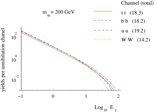
Figure 1: Differential photon yield $dN_{\gamma}/dE_{\gamma}$ for several annihilation channels, using a WIMP with mass $m_{w}=200$ GeV. The total photon yield for each channel is also shown in parenthesis.

2.2 Particle physics contribution

Concerning the particle physics contribution to the gamma–ray flux (2.3), one has all the other factors in front of $\bar{J}(\Delta\Omega)$. Their values will depend on the specific theoretical scenario where the WIMPs are embedded. With respect to the differential photon yield, it is known that this shows scaling properties [14], i.e. it depends only on the scaled variable $x=E_{\gamma}/m_{w}$, where $m_{w}$ is the mass of the WIMP. Thus can be reasonably parameterised for each possible annihilation channel of the WIMPs [14, 10]. For example, assuming that WIMPs annihilate producing $WW$, $ZZ$, $b\overline{b}$, $t\overline{t}$, and $u\overline{u}$, one can write $dN_{\gamma}/dx=ae^{-bx}/x^{1.5}$, with $(a,b)=(0.73,7.76)$ for the annihilation channels $WW$ and $ZZ$ [10, 42], $(1.0,10.7)$ for $b\overline{b}$, $(1.1,15.1)$ for $t\overline{t}$, and $(0.95,6.5)$ for $u\overline{u}$ [4]. In fact, the spectrum of gamma-rays is very close for all the above channels as illustrated in Fig. 1, except in the case $\tau^{+}\tau^{-}$ which produces smaller values (see e.g. [14, 16]). In our computation of the gamma-ray flux below we use the more exact PYTHIA fragmentation Monte Carlo [43].

On the other hand, the influence of the theoretical framework is crucial for the value of the annihilation cross section $\sigma_{i}$. As mentioned in the Introduction, we will work in the context of the simplest SUSY construction, where the lightest supersymmetric particle (LSP) is absolutely stable, and therefore a candidate for dark matter. It is remarkable that in most of the parameter space of this construction the LSP is an electrically neutral (also with no strong interactions) particle, called neutralino. This is welcome since otherwise the LSP would bind to nuclei and would be excluded as a candidate for dark matter from unsuccessful searches for exotic heavy isotopes.

As a matter of fact, there are four neutralinos, $\tilde{\chi}^{0}_{i}~{}(i=1,2,3,4)$, since they are the physical superpositions of the fermionic partners of the neutral electroweak gauge bosons, called bino ($\tilde{B}^{0}$) and wino ($\tilde{W}_{3}^{0}$), and of the fermionic partners of the neutral Higgs bosons, called Higgsinos ($\tilde{H}^{0}_{u}$, $\tilde{H}_{d}^{0}$). Therefore the lightest neutralino, $\tilde{\chi}^{0}_{1}$, will be the dark matter candidate. In the basis ($\tilde{B}^{0}$, $\tilde{W}_{3}^{0}$, $\tilde{H}_{u}^{0}$, $\tilde{H}_{d}^{0}$), the neutralino mass matrix is given by

$${\cal M}_{N}=\left(\begin{array}[]{cccc}M_{1}&0&-m_{Z}\cos\beta\sin\theta_{W}&m_{Z}\sin\beta\sin\theta_{W}\\ 0&M_{2}&m_{Z}\cos\beta\cos\theta_{W}&-m_{Z}\sin\beta\cos\theta_{W}\\ -m_{Z}\cos\beta\sin\theta_{W}&m_{Z}\cos\beta\cos\theta_{W}&0&-\mu\\ m_{Z}\sin\beta\sin\theta_{W}&-m_{Z}\sin\beta\cos\theta_{W}&-\mu&0\end{array}\right)\;,$$ (2.7)

where $M_{1}$ and $M_{2}$ are the bino and wino masses respectively, $\mu$ is the Higgsino mass parameter and $\tan\beta=\langle H_{u}^{0}\rangle/\langle H_{d}^{0}\rangle$ is the ratio of Higgs vacuum expectation values. This can be diagonalized by a matrix $Z$ such that we can express the lightest neutralino as

$$\tilde{\chi}^{0}_{1}={Z_{11}}\tilde{B}^{0}+{Z_{12}}\tilde{W}_{3}^{0}+{Z_{13}}\tilde{H}^{0}_{d}+{Z_{14}}\tilde{H}^{0}_{u}\ .$$ (2.8)

It is commonly defined that $\tilde{\chi}^{0}_{1}$ is mostly gaugino-like if $P\equiv|{Z_{11}}|^{2}+|{Z_{12}}|^{2}>0.9$, Higgsino-like if $P<0.1$, and mixed otherwise.

In Fig. 2 we show the relevant Feynman diagrams contributing to neutralino annihilation. As we will see, the cross section can be significantly enhanced depending on the SUSY model under consideration. We will concentrate here on the SUGRA scenario, where the soft terms are determined at the unification scale, $M_{GUT}\approx 2\times 10^{16}$ GeV, after SUSY breaking, and radiative electroweak symmetry breaking is imposed.

Let us start reviewing the situation in the case of mSUGRA, where the soft terms are assumed to be universal.

                                                            

$\propto\frac{m_{\chi}m_{f}}{m_{\tilde{f}}^{2}}Z_{11}^{2}~{}~{}~{}$ $\propto\frac{m_{\chi}^{2}}{m_{A}^{2}}\frac{Z_{11}Z_{13,14}}{m_{W}}m_{f_{d}}\tan\beta(\frac{m_{f_{u}}}{\tan\beta})~{}~{}~{}$ $\propto\frac{m_{f}m_{\chi}}{m_{Z}^{2}}Z_{13,14}^{2}~{}$ $\propto\frac{[-Z_{14}V_{21}^{*}+\sqrt{2}Z_{12}V_{11}^{*}]^{2}(-Z_{13}N_{31}^{*}+Z_{14}N_{41}^{*})^{2}}{1+m_{\chi_{i}^{+(0)}}^{2}/m_{\chi}^{2}-m_{W(Z)}^{2}/m_{\chi}^{2}}$

Figure 2: Dominant neutralino annihilation diagrams. Relevant parts of the amplitudes are shown explicitly Terms between parenthesis correspond to $f_{u}$ and $Z$ final states in second and fourth diagrams. V and N are chargino and neutralino mixing matrices.

3 mSUGRA predictions for the gamma-ray flux

Let us first recall that in mSUGRA one has only four free parameters defined at the GUT scale: the soft scalar mass $m$, the soft gaugino mass $M$, the soft trilinear coupling $A$, and $\tan\beta$. In addition, the sign of the Higgsino mass parameter, $\mu$, remains also undetermined by the minimization of the Higgs potential, which at tree level implies

$$\mu^{2}=\frac{m_{H_{d}}^{2}-m_{H_{u}}^{2}\tan^{2}\beta}{\tan^{2}\beta-1}-\frac{1}{2}M_{Z}^{2}\ .$$ (3.9)

As is well known, in this scenario the lightest neutralino is mainly bino [44, 45]. To understand this result qualitatively recall the evolution of $m_{H_{u}}^{2}$ towards generically large and negative values with the scale. Since $\mu^{2}$ given by Eq. (3.9), for reasonable values of $\tan\beta$, can be approximated as,

$$\mu^{2}\approx-m_{H_{u}}^{2}-\frac{1}{2}M_{Z}^{2}\ ,$$ (3.10)

then it becomes also large. In particular, $|\mu|$ becomes much larger than $M_{1}$ and $M_{2}$. Thus, as can be easily understood from Eqs. (2.7) and (2.8), the lightest neutralino will be mainly gaugino, and in particular bino, since at low energy $M_{1}=\frac{5}{3}\tan^{2}\theta_{W}M_{2}\approx 0.5M_{2}$.

Now, using Eq. (2.3) one can compute the gamma-ray flux for different values of the parameters. As a consequence of the $\tilde{\chi}^{0}_{1}$ being mainly bino, the predicted $\sigma_{i}$ is small, and therefore the flux is below the present accessible experimental regions. Note that only ${Z_{11}}$ is large and then the contribution of diagrams in Fig. 2 will be generically small. In addition, the (tree-level) mass of the CP-odd Higgs, $A$,

$$m^{2}_{A}=m_{H_{d}}^{2}+m_{H_{u}}^{2}+2\mu^{2}\ ,$$ (3.11)

will be large. The previous formula can be rewritten as

$$m^{2}_{A}\approx m_{H_{d}}^{2}-m_{H_{u}}^{2}-M_{Z}^{2}\ ,$$ (3.12)

where Eq. (3.10) has been used. As mentioned above, $m_{H_{u}}^{2}$ evolves at low energy towards large and negative values, producing a large value for $m_{A}$, and therefore a further suppression in the annihilation channels.

This fact is shown in Fig. 3 using the DarkSUSY program [46]. There, contours of the gamma-ray flux $\Phi_{\gamma}$ in the parameter space ($m$, $M$) for $\tan\beta=5$, $A=0$ and $\mu>0$ are plotted, using the complete one-loop corrected effective potential. We will not consider in the calculation the opposite sign of $\mu$ because this would produce a negative contribution for the $g_{\mu}-2$, and, as will be discussed below, we are mainly interested in positive contributions. Recall that the sign of the contribution is basically given by $\mu M_{2}$, and that $M$, and therefore $M_{2}$, can always be made positive after performing an $U(1)_{R}$ rotation. As input for the top mass, $m_{t}(pole)=175$ GeV has been used.

In the computation we are using a NFW profile with $\Delta\Omega=10^{-3}$ sr, and recent experimental and astrophysical constraints are taken into account. In particular, the lower bounds on the masses of the supersymmetric particles and on the lightest Higgs have been implemented, as well as the experimental bounds on the branching ratio of the $b\to s\gamma$ process and on $a^{\rm SUSY}_{\mu}$. Due to its relevance, the effect of the WMAP constraint on the dark matter relic density is shown explicitly.

Concerning $a^{\rm SUSY}_{\mu}$, we have taken into account the recent experimental result for the muon anomalous magnetic moment [50], as well as the most recent theoretical evaluations of the Standard Model contributions [51]. It is found that when $e^{+}e^{-}$ data are used the experimental excess in $(g_{\mu}-2)$ would constrain a possible supersymmetric contribution to be $a^{\rm SUSY}_{\mu}=(27.1\pm 10)\times 10^{-10}$. At $2\sigma$ level this implies $7.1\times 10^{-10}\raise 1.29167pt\hbox{$\;<$\kern-7.5pt\raise-4.73611pt\hbox{$\sim\;$}}a^{\rm SUSY}_{\mu}\raise 1.29167pt\hbox{$\;<$\kern-7.5pt\raise-4.73611pt\hbox{$\sim\;$}}47.1\times 10^{-10}$. It is worth noticing here that when tau data are used a smaller discrepancy with the experimental measurement is found. In order not to exclude the latter possibility we will discuss the relevant value $a^{\rm SUSY}_{\mu}=7.1\times 10^{-10}$ in the figures throughout the paper. The region of the parameter space to the right of this line will be forbidden (allowed) if one consider electron (tau) data.

On the other hand, the measurements of $B\to X_{s}\gamma$ decays at CLEO [52] and BELLE [53], lead to bounds on the branching ratio $b\to s\gamma$. In particular we impose on our computation $2.33\times 10^{-4}\leq BR(b\to s\gamma)\leq 4.15\times 10^{-4}$, where the evaluation is carried out using the routine provided by the program micrOMEGAs [48]. This program is also used for our evaluation of $a^{\rm SUSY}_{\mu}$ and relic neutralino density.

As we can see in Fig. 3, the points corresponding to a sufficiently low relic neutralino density, and satisfying the Higgs mass bound in mSUGRA, $m_{h}>114$ GeV, are located in the narrow coannihilation branch of the parameter space, i.e. the region where the stau is the next to the LSP producing efficient coannihilations. For these points the neutralino mass is larger than the top mass (note that we can deduce its value in the plot from the value of $M$, since in mSUGRA $m_{\tilde{\chi}^{0}_{1}}\simeq{M_{1}}\simeq 0.4\ M$ implying $m_{\tilde{\chi}^{0}_{1}}\raise 1.29167pt\hbox{$\;>$\kern-7.5pt\raise-4.73611pt\hbox{$\sim\;$}}200$ GeV), and $t\overline{t}$ final states are allowed. In fact, through the $A$-exchange channel, these are the main source of the gamma-ray flux. The contribution from $b\overline{b}$ states is also relevant, and the relation between both contributions can be obtained taking into account that (see Fig. 2) $\sigma_{A}(t\overline{t})\propto\beta_{t}m_{t}^{2}/\tan^{2}\beta$, $\sigma_{A}(b\overline{b})\propto\beta_{b}m_{b}^{2}\tan^{2}\beta$, with $\beta_{f}=\sqrt{1-m_{f}^{2}/m_{\chi}^{2}}$, and therefore $\sigma_{A}(t\overline{t})/\sigma_{A}(b\overline{b})\sim\frac{1}{\tan^{4}\beta}(m_{t}/m_{b})^{2}$ for sufficiently large neutralino mass. In particular, for $\tan\beta=5$ one obtains $\sigma_{A}(t\overline{t})/\sigma_{A}(b\overline{b})\sim 2$. There is of course the possibility of $\tau\overline{\tau}$ final states, but their contributions are negligible compared with the $b\overline{b}$ ones. Note that, following the above arguments, $\sigma_{A}(\tau\overline{\tau})/\sigma_{A}(b\overline{b})\sim\frac{1}{3}(m_{\tau}/m_{b})^{2}\sim 0.05$, where 3 is a colour factor.

Let us finally remark that if we impose consistency with the $e^{+}e^{-}$ data concerning $(g_{\mu}-2)$, the whole parameter space would be excluded (notice that the region to the right of the black dashed line in Fig. 3 corresponds to $a^{\rm SUSY}_{\mu}<7.1\times 10^{-10}$).

We summarize the above results in Fig. 4, using the same parameter space as in Fig. 3. There, the values of $\Phi_{\gamma}$ allowed by all experimental constraints as a function of the neutralino mass $m_{\tilde{\chi}^{0}_{1}}$ are depicted. Points shown with black stars have $0.094<\Omega_{\tilde{\chi}^{0}_{1}}h^{2}<0.129$, and are therefore favoured by WMAP. Points with $0.129<\Omega_{\tilde{\chi}^{0}_{1}}h^{2}<0.3$ are shown with light grey (magenta) triangles. We also consider the possibility that not all the dark matter is made of neutralinos, allowing $0.03<\Omega_{\tilde{\chi}^{0}_{1}}h^{2}<0.094$. In this case we have to rescale the density of neutralinos in the galaxy $\rho(r)$ in Eqs. (2.5) and (2.6) by a factor $\Omega_{\tilde{\chi}^{0}_{1}}h^{2}/0.094$. Points corresponding to this possibility are shown with dark grey (blue) boxes.

We observe that, generically, the gamma-ray flux for a threshold of 1 GeV (left frame) is constrained to be $\Phi_{\gamma}\raise 1.29167pt\hbox{$\;<$\kern-7.5pt\raise-4.73611pt\hbox{$\sim\;$}}10^{-11}$ cm^-2 s^-1. Obviously, in this mSUGRA scenario with $\tan\beta=$ 5 the EGRET data cannot be reproduced, and more sensitive detectors producing further data are needed. Note that GLAST experiment, where values of the gamma-ray flux as low as $10^{-10}$ cm^-2 s^-1 will be accessible, is not sufficient. For atmospheric telescopes, such as HESS, the situation is similar, as can be seen in the plot on the right frame.

The annihilation cross section can be increased, and therefore the gamma-ray flux, when the value of $\tan\beta$ is increased. Notice for instance that the contribution of the $b\overline{b}$ final state, which is proportional to $\tan^{2}\beta$ is now more important than the $t\overline{t}$ one. For example, for $\tan\beta=35$, using the above approximation one obtains $\sigma_{A}(t\overline{t})/\sigma_{A}(b\overline{b})\approx\frac{1}{35^{4}}(m_{t}/m_{b})^{2}\sim 10^{-3}$. In addition, the bottom Yukawa coupling increases, and as a consequence $m_{H_{d}}^{2}$ decreases, implying that $m^{2}_{A}$, given by Eq. (3.12), also decreases. Indeed, annihilation channels through $A$ exchange are more important now and their contributions to the flux will increase it. This effect is shown in Fig. 6, which can be compared with Fig. 3.

The above results concerning the gamma-ray flux are summarized in Fig. 6. There we see that the flux for a threshold of 1 GeV is larger than for $\tan\beta=$5. In any case, only a very small region of the parameter space turns out to be accessible for GLAST, and no region for HESS. It is worth noticing that now only the lower areas bounded by the dashed line correspond to $a^{\rm SUSY}_{\mu}<7.1\times 10^{-10}$, and therefore would be excluded by ($g_{\mu}-2$) if we impose consistency with the $e^{+}e^{-}$ data.

We have also analyzed very large values of $\tan\beta$, such as 50. In this case, still EGRET data cannot be reproduced, but larger regions of the parameter space would be accessible for GLAST and also HESS. In particular, fluxes with $\Phi_{\gamma}\raise 1.29167pt\hbox{$\;<$\kern-7.5pt\raise-4.73611pt\hbox{$\sim\;$}}10^{-9}$ cm^-2 s^-1 ($\Phi_{\gamma}\raise 1.29167pt\hbox{$\;<$\kern-7.5pt\raise-4.73611pt\hbox{$\sim\;$}}10^{-11}$ cm^-2 s^-1) can be obtained for a threshold of 1 GeV (60 GeV).

Let us finally remark that the result obtained above concerning EGRET, should be expected given the following argument. The relic density can be approximated in the simplest situation, when the annihilation cross section is velocity independent, as $\Omega h^{2}\sim\frac{3\times 10^{-27}\mathrm{cm^{3}s^{-1}}}{<\sigma v>}$. This implies that in order to obtain the result $\Omega h^{2}\sim 0.1$ one needs a cross section $\sigma v\sim 3\times 10^{-26}\mathrm{cm^{3}s^{-1}}$. Using this value for the annihilation cross section in the galaxy in Eq. (2.3), for a NFW profile with $\overline{J}\left(10^{-3}\right)\approx 3\times 10^{3}$ and a photon yield of about 10 as can be deduced from Fig. 1, one obtains a gamma-ray flux $\Phi_{\gamma}\sim 10^{-9}$ cm^-2 s^-1, i.e. below EGRET sensitivity. In fact, the value of the flux is typically two or three orders of magnitude smaller than this estimation, since in the early Universe coannihilations can also contribute to $\sigma v$ as discussed above, thus $3\times 10^{-26}\mathrm{cm^{3}s^{-1}}$ can be considered as an upper limit. The results shown in Figs. 4 and 6 confirm this rough discussion.

Figure 3: Gamma-ray flux $\Phi_{\gamma}$ for a threshold of 1 GeV, in the parameter space of the mSUGRA scenario ($m$, $M$) for $\tan\beta=5$, $A=0$ and $\mu>0$. The dot-dashed curves are contours of $\Phi_{\gamma}$ in cm^-2 s^-1 units. A NFW profile is used with $\Delta\Omega=10^{-3}$ sr. The region to the left of the light grey (green) dashed line is excluded by the lower bound on the Higgs mass. The region to the left of the dotted line is excluded by the lower bound on the chargino mass $m_{\tilde{\chi}_{1}^{\pm}}>103$ GeV. The region to the right of the black dashed line corresponds to $a^{\rm SUSY}_{\mu}<7.1\times 10^{-10}$, and would be excluded by $e^{+}e^{-}$ data. The region at the bottom (Stau LSP) is excluded because the lightest stau is the LSP. The dark grey (red) region fulfils $0.1\leq\Omega_{\tilde{\chi}_{1}^{0}}h^{2}\leq 0.3$ (the black region on top of this indicates the WMAP range $0.094<\Omega_{\tilde{\chi}_{1}^{0}}h^{2}<0.129$).

         

Figure 4: Scatter plot of the gamma-ray flux $\Phi_{\gamma}$ for a threshold of 1 GeV (left), and 60 GeV (right), as a function of the neutralino mass $m_{\chi}$, using the same parameter space as in Fig. 3, for $\tan\beta=5$, $A=0$ and $\mu>0$. All points have $a^{\rm SUSY}_{\mu}<7.1\times 10^{-10}$, and therefore would be excluded by ($g_{\mu}-2$) if we impose consistency with the $e^{+}e^{-}$ data. They fulfil all other experimental constraints, and those depicted with light grey (magenta) triangles have $0.129<\Omega_{\tilde{\chi}^{0}_{1}}h^{2}<0.3$, with black stars have $0.094<\Omega_{\tilde{\chi}^{0}_{1}}h^{2}<0.129$, and finally with dark grey (blue) boxes have $0.03<\Omega_{\tilde{\chi}^{0}_{1}}h^{2}<0.094$ with the appropriate rescaling of the density of neutralinos in the galaxy as discussed in the text. From top to bottom, the first solid line in the left frame corresponds to the signal reported by EGRET, and the upper area bounded by the second solid line will be analyzed by GLAST experiment (HESS experiment in the right frame).

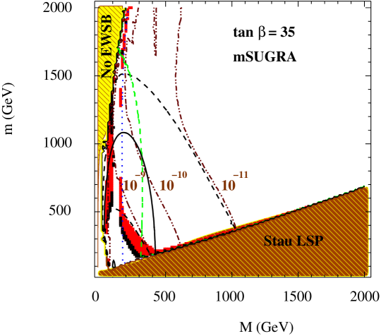
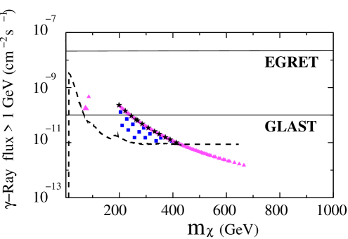
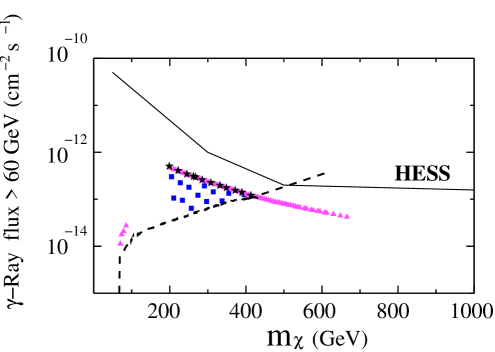
Figure 5: The same as in Fig. 3 but for tan$\beta$=35. The region to the left of the solid line is excluded by $b\to s\gamma$.

         

Figure 6: The same as in Fig. 4 but for tan$\beta$=35. Now, only the lower areas bounded by the dashed line correspond to $a^{\rm SUSY}_{\mu}<7.1\times 10^{-10}$, and therefore would be excluded by ($g_{\mu}-2$) if we impose consistency with the $e^{+}e^{-}$ data.

4 Departures from mSUGRA

As discussed in detail in Refs. [54, 55, 56] in the context of direct detection, the neutralino-proton scattering cross section can be increased in different ways when the structure of mSUGRA for the soft terms is abandoned. Since the diagrams for neutralino annihilation through neutral Higgs exchange are related to those by crossing symmetry, we can use the same arguments here. In particular, it is possible to enhance the annihilation channels involving exchange of the CP-odd Higgs, $A$, by reducing the Higgs mass, and also by increasing the Higgsino components of the lightest neutralino. As a consequence, the gamma-ray flux will be increased. A brief analysis based on the Higgs mass parameters, $m_{H_{d}}^{2}$ and $m_{H_{u}}^{2}$, at the electroweak scale can clearly show how these effects can be achieved.

First, a decrease in the value of the mass of $A$ can be obtained by increasing $m_{H_{u}}^{2}$ (i.e., making it less negative) and/or decreasing $m_{H_{d}}^{2}$. This is easily understood from Eq. (3.12).

Second, through the increase in the value of $m_{H_{u}}^{2}$ an increase in the Higgsino components of the lightest neutralino can also be achieved. Making $m_{H_{u}}^{2}$ less negative, its positive contribution to $\mu^{2}$ in (3.10) would be smaller. Eventually $|\mu|$ will be of the order of $M_{1}$, $M_{2}$ and $\tilde{\chi}_{1}^{0}$ will then be a mixed Higgsino-gaugino state. Thus annihilation channels through Higgs exchange become more important than in mSUGRA, where $|\mu|$ is large and $\tilde{\chi}_{1}^{0}$ is mainly bino. This is also the case for $Z$-, $\chi_{1}^{\pm}$-, and $\tilde{\chi}_{1}^{0}$-exchange channels.

As pointed out in Refs. [54, 55, 56], non-universal soft parameters can produce the above mentioned effects. Let us first consider non-universalities in the scalar masses.

4.1 Non-universal scalars

We can parameterise the non-universalities in the Higgs sector, at the GUT scale, as follows:

$$m_{H_{d}}^{2}=m^{2}(1+\delta_{1})\ ,\quad m_{H_{u}}^{2}=m^{2}(1+\delta_{2})\ .$$ (4.13)

Concerning squarks and sleptons we will assume that the three generations have the same mass structure:

$$m_{Q_{L}}^{2} = m^{2}(1+\delta_{3})\ ,\quad m_{u_{R}}^{2}=m^{2}(1+\delta_{4})\ ,$$

$$m_{e_{R}}^{2} = m^{2}(1+\delta_{5})\ ,\quad m_{d_{R}}^{2}=m^{2}(1+\delta_{6})\ ,$$

$$m_{L_{L}}^{2} = m^{2}(1+\delta_{7})\ .$$ (4.14)

Such a structure avoids potential problems with flavour changing neutral currents. Note also that whereas $\delta_{i}\geq-1$, $i=3,...,7$, in order to avoid an unbounded from below (UFB) direction breaking charge and colour, $\delta_{1,2}\leq-1$ is possible as long as $m_{1}^{2}\,=\,m_{H_{d}}^{2}+\mu^{2}>0$ and $m_{2}^{2}\,=\,m_{H_{u}}^{2}+\mu^{2}>0$ are fulfilled.

An increase in $m_{H_{u}}^{2}$ at the electroweak scale can be obviously achieved by increasing its value at the GUT scale, i.e., with the choice $\delta_{2}>0$. In addition, this is also produced when $m_{Q_{L}}^{2}$ and $m_{u_{R}}^{2}$ at $M_{GUT}$ decrease, i.e. taking $\delta_{3,4}<0$, due to their (negative) contribution proportional to the top Yukawa coupling in the renormalization group equation (RGE) of $m_{H_{u}}^{2}$. Similarly, a decrease in the value of $m_{H_{d}}^{2}$ at the electroweak scale can be obtained by decreasing it at the GUT scale with $\delta_{1}<0$. Also, this effect is produced when $m_{Q_{L}}^{2}$ and $m_{d_{R}}^{2}$ at $M_{GUT}$ increase, due to their (negative) contribution proportional to the bottom Yukawa coupling in the RGE of $m_{H_{d}}^{2}$. Thus one can deduce that $m^{2}_{A}$ will be reduced by choosing also $\delta_{3,6}>0$. In fact non-universality in the Higgs sector gives the most important effect, and including the one in the sfermion sector the annihilation cross section only increases slightly. Thus in what follows we will take $\delta_{i}=0$, $i=3,...,7$. Let us analyze then three representative cases:

$$a)\,\,\delta_{1} = 0\ \,\,\,\,\,\,\,\,,\,\,\,\,\delta_{2}\ =\ 1\ ,$$

$$b)\,\,\delta_{1} = -1\ \,\,\,\,,\,\,\,\,\delta_{2}\ =\ 0\ ,$$

$$c)\,\,\delta_{1} = -1\ \,\,\,\,,\,\,\,\delta_{2}\ =\ 1\ .$$ (4.15)

Clearly, the above discussion about decreasing $\mu^{2}$ applies well to case a), where the variation in $m_{H_{u}}^{2}$ through $\delta_{2}$ is relevant. This is shown in Fig. 8 for $\tan\beta=5$ and $A=0$, which can be compared with Fig. 3. Note that now there is an important area in the upper left (no EWSB) where $\mu^{2}$ becomes negative due to the increasing in $\delta_{2}$ with respect to the universal case. We see that the decrease of the $\mu$ parameter opens a new allowed (narrow) region of the parameter space, close to this one. In particular, the value of the relic density $\Omega_{\tilde{\chi}^{0}_{1}}$ is affected due to the increase of the Higgsino components of ${\tilde{\chi}^{0}_{1}}$ with respect to the dominant bino component of the universal case. Thus the relic abundance is placed inside the astrophysical bounds. In Fig. 2 we can see that this nature of the LSP enhances the neutralino coupling to the $Z$ (giving rise to bottom and top final states when kinematically allowed), and to the lightest chargino $\chi_{1}^{\pm}$ and neutralino $\tilde{\chi}_{1}^{0}$ (inducing $W^{\pm}W^{\pm}$ and $ZZ$ boson final states, especially for low values of $M$).

We can see the enhancement in the gamma-ray flux in Fig. 8, where many points accessible for GLAST and HESS are obtained. This can be compared with the result of Fig. 4 for the universal scenario, where such points are not possible with $\tan\beta=5$. On the other hand, the lower region, below GLAST (and HESS), corresponds to the narrow coannihilation branch. In this case the neutralino is mainly bino and the discussion of this region for mSUGRA in the previous section applies also here.

Let us remark, however, that if we impose consistency with the $e^{+}e^{-}$ data concerning $(g_{\mu}-2)$, the whole parameter space would be excluded (notice that the region to the right of the black dashed line in Fig. 8 corresponds to $a^{\rm SUSY}_{\mu}<7.1\times 10^{-10}$), as in the case of mSUGRA.

For $\tan\beta=35$, one can see in Figs. 10 and 10 the enhancement of the flux related to the coannihilation branch. As discussed in the previous section for mSUGRA, the increase is about two orders of magnitude with respect to the case $\tan\beta=5$ (see Fig. 8), as expected by the couplings proportionals to tan$\beta$ in the $A$-exchange channels. On the other hand, one can also see in Fig. 10 that the flux in the Higgsino branch does not increase significantly. This is because it is mainly produced by the $Z$ exchange that does not depend on tan$\beta$ at all. Concerning this branch, it is worth noticing that it is not so close to the no EWSB area as in the case of mSUGRA. In particular, one can see in Fig. 10 that larger values of the parameters imply a larger gap between the Higgsino branch and the no EWSB area. Compare for example the points with $m$=1000 GeV and 2000 GeV, and with the relic density inside the astrophysical bounds. In order to obtain the same value of the relic density, for $m$=2000 GeV a higher value of $\mu$ is necessary.

It is worth noticing that now, unlike the $\tan\beta=5$ case, not all points would be excluded by ($g_{\mu}-2$) if we impose consistency with the $e^{+}e^{-}$ data. In Fig. 10 those to the left of the dashed line correspond to $a^{\rm SUSY}_{\mu}>7.1\times 10^{-10}$, and therefore would be allowed on this ground.

On the other hand, for case b) with $\tan\beta=5$, studied in Figs. 12 and 12, the only region which is allowed by the experimental constraints is the one corresponding to the narrow coannihilation branch. Recall that now $m_{H_{u}}^{2}$ is not varied and therefore the effect of decreasing $\mu^{2}$ is not present. As in the case of mSUGRA, the gamma-ray flux is small and below the accessible experimental areas. However, for $\tan\beta=35$, due to the effect of decreasing $m_{H_{d}}^{2}$ significantly, $m_{A}^{2}$ can be very small. Notice the area in the upper left of Fig. 14 where $m_{A}^{2}$ becomes negative. As a consequence, Fig. 14 shows similar fluxes to those of the case a) in Fig. 10, but with a larger contribution from the $A$ exchange. Thus interesting regions of the parameter space are accessible for future experiments.

Now we can see in Fig. 14 (and Fig. 14) that there are two cosmologically allowed corridors. This can be easily understood from the variation in $m_{A}$. For example, in Fig. 14, for a given value of $m$, and from large to small $M$, $m_{A}$ decreases. Starting with $M=2000$ GeV, one has $m_{A}>2m_{\tilde{\chi}^{0}_{1}}$, and therefore a small annihilation cross section producing a large relic density. However, when $m_{A}$ becomes close to $2m_{\tilde{\chi}^{0}_{1}}$ the annihilation cross section increases and therefore the relic density decreases entering in the first allowed corridor with $0.094<\Omega_{\tilde{\chi}^{0}_{1}}h^{2}<0.3$. For slightly smaller values of $M$ one finally arrives to the A-pole region where $m_{A}\sim 2m_{\tilde{\chi}^{0}_{1}}$ and the relic density is too small. Smaller values of $m_{A}$ close this region, producing a decrease in the annihilation cross section, which allows to enter in the second corridor with the relic density inside the observational bounds. For $m_{A}$ too small this second corridor is closed, and the relic density is too large, $\Omega_{\tilde{\chi}^{0}_{1}}h^{2}>0.3$. Finally, one arrives to the region where $m_{A}^{2}$ becomes negative.

Concerning case c), this is basically a combination of the previous two cases, a) and b). In Fig. 16 one can see that the region where the neutralino is mainly Higgsino is already open at tan$\beta=5$. This is of course due to the non-universality of $m_{H_{u}}$. Consequently, large fluxes can be obtained, as shown in Fig. 16. These figures are qualitatively similar to those corresponding to case a) with tan$\beta=5$, Figs. 8 and 8. Moreover, one can see in Fig. 18 and 18 for tan$\beta=35$ that the $A$ contribution is now also largely present, although the effect of the Higgsino component of the neutralino is also important in the region $m,M~{}\sim$ 500 GeV. Notice that the shape of the allowed corridors is qualitatively similar to that corresponding to case b), Figs. 14 and 14,

Let us also mention that the combination of both non-universalities gives rise to very light Higgses, particularly charged Higgses, and that new final states ($H^{+}W^{-}$ or $ZH$) can be kinematically allowed and even reach 30% of the branching ratio in some regions of the parameter space. This effect is not possible in mSUGRA.

Finally, we have also analyzed very large values of tan$\beta$, such as 50, for cases a), b), and c). The results are qualitatively similar, in the sense that many points accessible for GLAST and HESS are obtained.

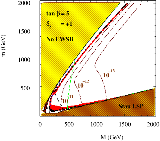
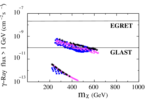
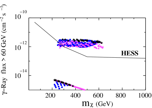
Figure 7: The same as in Fig. 3 but for the non-universal scalar case a) $\delta_{1}=0$, $\delta_{2}=1$, discussed in Eq. (4.15).

       

Figure 8: The same as in Fig. 4 but for the non-universal scalar case a) $\delta_{1}=0$, $\delta_{2}=1$, discussed in Eq. (4.15).

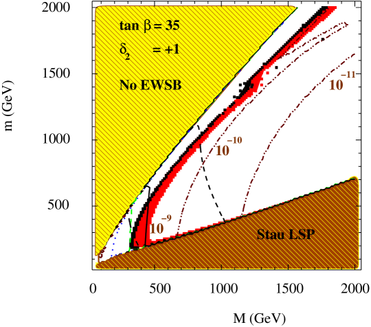
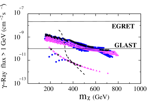
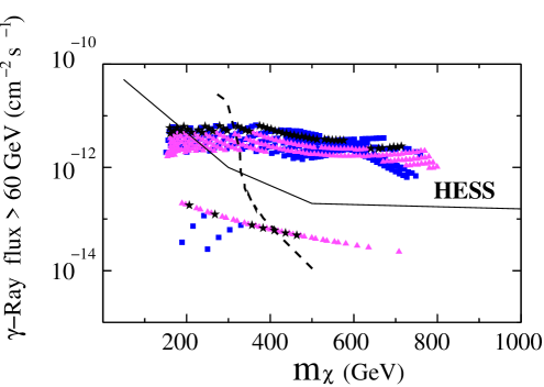
Figure 9: The same as in Fig. 3 but for $\tan\beta=$35 and the non-universal scalar case a) $\delta_{1}=0$, $\delta_{2}=1$, discussed in Eq. (4.15). The region to the left of the solid line is excluded by $b\to s\gamma$.

         

Figure 10: The same as in Fig. 4 but for $\tan\beta=$35 and the non-universal scalar case a) $\delta_{1}=0$, $\delta_{2}=1$, discussed in Eq. (4.15). Now, the region to the right of the dashed line corresponds to $a^{\rm SUSY}_{\mu}<7.1\times 10^{-10}$, and would be excluded by $e^{+}e^{-}$ data.

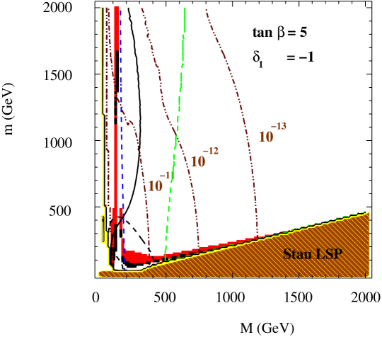
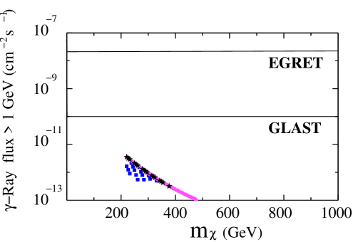
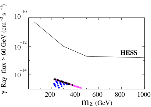
Figure 11: The same as in Fig. 3 but for the non-universal scalar case b) $\delta_{1}=-1$, $\delta_{2}=0$, discussed in Eq. (4.15). The region to the left of the solid line is excluded by $b\to s\gamma$.

       

Figure 12: The same as in Fig. 4 but for the non-universal scalar case b) $\delta_{1}=-1$, $\delta_{2}=0$, discussed in Eq. (4.15).

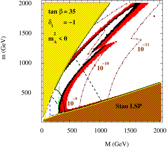
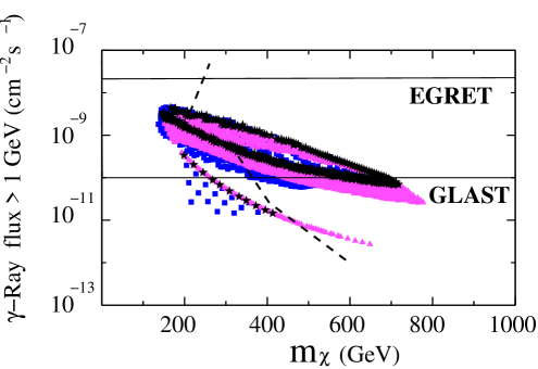
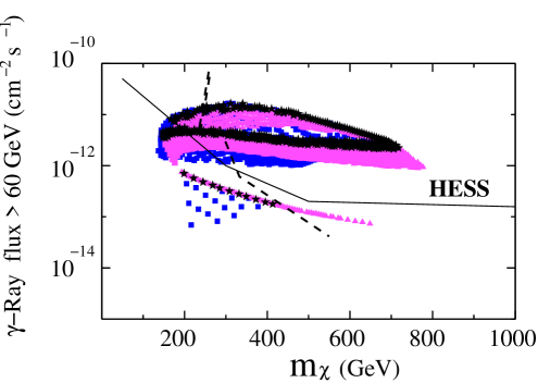
Figure 13: The same as in Fig. 3 but for $\tan\beta=35$ and the non-universal scalar case b) $\delta_{1}=-1$, $\delta_{2}=0$, discussed in Eq. (4.15). The region to the left of the solid line is excluded by $b\to s\gamma$.

         

Figure 14: The same as in Fig. 4 but for $\tan\beta=35$ and the non-universal scalar case b) $\delta_{1}=-1$, $\delta_{2}=0$, discussed in Eq. (4.15). Now, the regions to the right of the dashed lines correspond to $a^{\rm SUSY}_{\mu}<7.1\times 10^{-10}$, and would be excluded by $e^{+}e^{-}$ data. These do not include the points with black stars between both dashed lines, which are allowed.

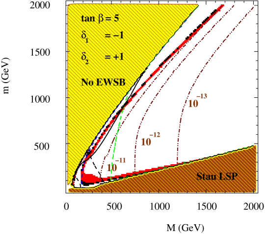
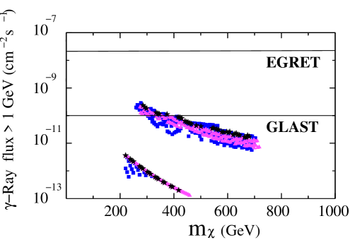
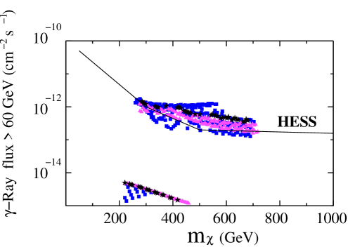
Figure 15: The same as in Fig. 3 but for the non-universal scalar case c) $\delta_{1}=-1$, $\delta_{2}=1$, discussed in Eq. (4.15). The region to the left of the solid line is excluded by $b\to s\gamma$.

         

Figure 16: The same as in Fig. 4 but for $\tan\beta=35$ and the non-universal scalar case c) $\delta_{1}=-1$, $\delta_{2}=1$, discussed in Eq. (4.15).

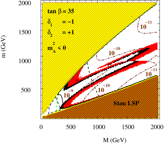
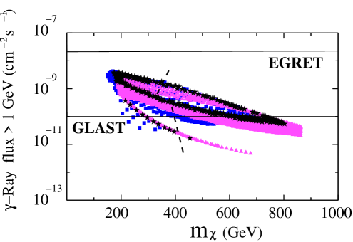
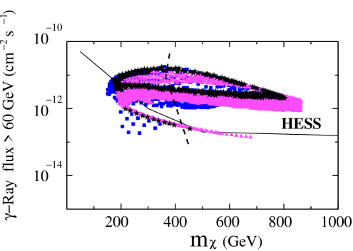
Figure 17: The same as in Fig. 3 but for $\tan\beta=35$ and the non-universal scalar case c) $\delta_{1}=-1$, $\delta_{2}=1$, discussed in Eq. (4.15). The region to the left of the solid line is excluded by $b\to s\gamma$.

       

Figure 18: The same as in Fig. 4 but for $\tan\beta=35$ and the non-universal scalar case c) $\delta_{1}=-1$, $\delta_{2}=1$, discussed in Eq. (4.15). Now, the regions to the right of the dashed lines correspond to $a^{\rm SUSY}_{\mu}<7.1\times 10^{-10}$, and would be excluded by $e^{+}e^{-}$ data. These do not include the points with black starts between both dashed lines, which are allowed.

4.2 Non-universal gauginos

Let us now study the effect of the non-universality in the gaugino masses. We can parameterise this as follows:

$$M_{1}=M\ ,\quad M_{2}=M(1+\delta^{\prime}_{2})\ ,\quad M_{3}=M(1+\delta^{\prime}_{3})\ ,$$ (4.16)

where $M_{1,2,3}$ are the bino, wino and gluino masses, respectively, and $\delta^{\prime}_{i}=0$ corresponds to the universal case.

In order to increase the annihilation cross section it is worth noticing that $M_{3}$ appears in the RGEs of squark masses. Thus the contribution of squark masses proportional to the top Yukawa coupling in the RGE of $m_{H_{u}}^{2}$ will do this less negative if $M_{3}$ is small. As discussed above, this produces a decrease in the value of $|\mu|$ and therefore a mixed Higgsino-gaugino lightest neutralino, which may help in order to increase the gamma-ray flux.

Because the mass of the lightest Higgs is very dependent on the value of $M_{3}$, through radiative corrections, its decrease is very limited. In fact, in order to satisfy the lower limit of $M_{3}$, $M$ in (4.16) may have to increase, thus rather than a decrease in $M_{3}$ what one obtains is an effective increase in $M_{1}$ and $M_{2}$, which leads to a larger (less negative) value of $m_{H_{u}}^{2}$ and thus a reduction in the value of $|\mu|$. This in turn implies heavier neutralinos, when the lightest neutralino is mostly gaugino, and an increase of the Higgsino composition, which would be dominant if $M_{1}>|\mu|$ at the electroweak scale. Finally, decreasing the ratio $M_{3}/M_{1}$ leads to a more efficient neutralino annihilation, due to the enhancement in the Higgsino components of $\tilde{\chi}_{1}^{0}$, entailing a reduction of $\Omega_{\tilde{\chi}^{0}_{1}}$.

In the following we analyze the case $\delta^{\prime}_{2}=0,\delta^{\prime}_{3}=-0.4$. Lower values of $M_{3}$ at the GUT scale cannot produce a sufficient amount of relic density. We show the situation for $\tan\beta=5$ in Fig. 20. Notice that the Higgs mass bound allows only the region corresponding to the narrow coannihilation branch. Thus the $A$-exchange channel is the relevant one here. The fact that in this case the gamma-ray flux is larger than in mSUGRA (one can compare Figs. 20 and 4) is due to the different composition of the neutralino. For example, for a point with $m=$ 200 GeV and $M=$ 1100 GeV (corresponding to $\Omega_{\chi}$=0.16) one obtains $Z_{13}=$ 0.11 in this non-universal case, whereas $Z_{13}=$ 0.04 in mSUGRA. Thus the Higgsino component of the neutralino is more important with non-universality.

In the large tan $\beta$ regime there is now a new feature. We can see in Fig. 22 that we have three cosmologically allowed corridors for $\tan\beta=35$. To analyze them, let us consider a fixed value of $m$, for example $m=1000$ GeV, and go from large to small $M$. For $M=2000$ GeV, $m_{A}$ is already smaller than $2m_{\tilde{\chi}^{0}_{1}}$ (this effect is not present for $\tan\beta=5$), producing a too large relic density. However, for smaller values of $M$ the decreasing in $m_{A}$ is not as steep as in non-universal scalar cases, and for $M\sim 1500$ GeV, $m_{A}$ becomes very close to $2m_{\tilde{\chi}^{0}_{1}}$. Thus the relic density is placed inside the bounds, $0.094<\Omega_{\tilde{\chi}^{0}_{1}}h^{2}<0.3$. For slightly smaller values of $M$ one arrives to the A-pole region since $m_{A}\sim 2m_{\tilde{\chi}^{0}_{1}}$, and the relic density is too small. If we continue to the left, $m_{A}>2m_{\tilde{\chi}^{0}_{1}}$, and this close the A-pole region producing a decrease in the annihilation cross section, which allows us to enter in the second corridor. Finally, the third corridor to the left of Fig. 22 is the usual Higgsino branch generated by the increase of the Higgsino components of the neutralino, near the noEWSB area where $\mu$ is small. As discussed in the case of Fig. 10, the gap between this branch and the no EWSB area increases with larger values of the parameters. See e.g. $m$=1500 GeV and 2000 GeV. It is also worth noticing that now, for a fixed value of $m$, there are more points with a relic density inside the astrophysical bounds. This is so because the value of $\mu$ is more stable with respect to variations in $M$. Note in this respect that here we are lowering $\mu$ through the value of $M_{3}$, and this is a loop effect.

Let us finally mention that in the latter region the $Z$-exchange channel dominates producing fluxes with $b\overline{b}$ final states ($t\overline{t}$ being kinematically disfavoured). This corresponds to $M$ smaller than about 900 GeV. The corridors related to the A-pole open for $M$ about 600 and 1000 GeV. These three corridors can be clearly distinguished in Fig. 22. The mixed Higgsino-gaugino one for $200\raise 1.29167pt\hbox{$\;<$\kern-7.5pt\raise-4.73611pt\hbox{$\sim\;$}}m_{\chi}\raise 1.29167pt\hbox{$\;<$\kern-7.5pt\raise-4.73611pt\hbox{$\sim\;$}}400$ GeV, and the other two for $300\raise 1.29167pt\hbox{$\;<$\kern-7.5pt\raise-4.73611pt\hbox{$\sim\;$}}m_{\chi}\raise 1.29167pt\hbox{$\;<$\kern-7.5pt\raise-4.73611pt\hbox{$\sim\;$}}900$ GeV and $450\raise 1.29167pt\hbox{$\;<$\kern-7.5pt\raise-4.73611pt\hbox{$\sim\;$}}m_{\chi}\raise 1.29167pt\hbox{$\;<$\kern-7.5pt\raise-4.73611pt\hbox{$\sim\;$}}900$ GeV. The latter gives rise to the largest flux. As in the case of non-universal scalars, we can observe in the figure that important regions of the parameter space will be accessible for future experiments.

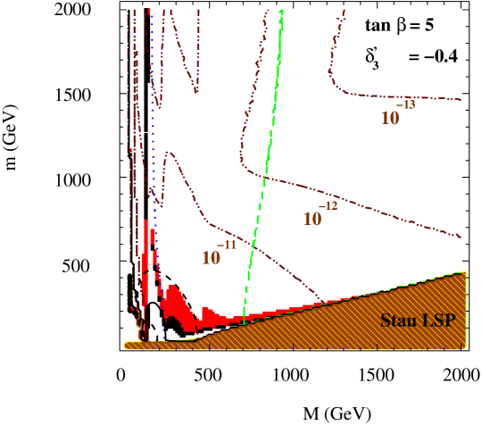
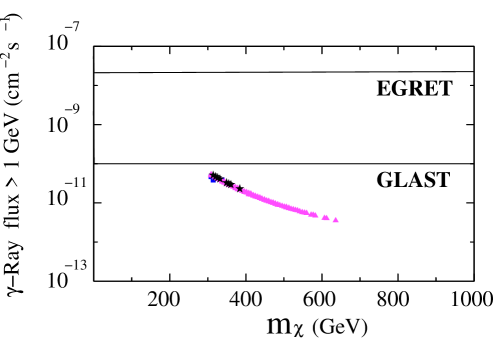
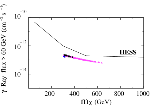
Figure 19: The same as in Fig. 3 but for the non-universal gaugino case $\delta_{3}^{\prime}=-0.4$, discussed in Eq. (4.16).

       

Figure 20: The same as in Fig. 4 but for the non-universal gaugino case $\delta_{3}^{\prime}=-0.4$, discussed in Eq. (4.16).

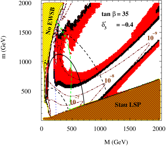
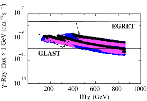
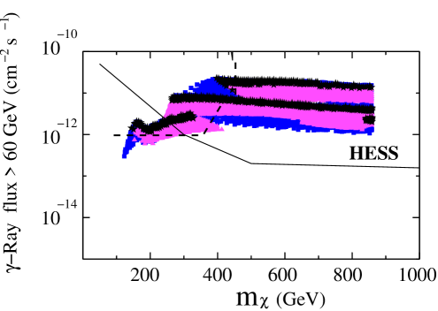
Figure 21: The same as in Fig. 3 but for $\tan\beta=35$ and the non-universal gaugino case $\delta_{3}^{\prime}=-0.4$, discussed in Eq. (4.16). The region to the left of the solid line is excluded by $b\to s\gamma$.

         

Figure 22: The same as in Fig. 4 but for $\tan\beta=35$ and the non-universal gaugino case $\delta_{3}^{\prime}=-0.4$, discussed in Eq. (4.16). Now, the regions to the right (and below) the dashed lines correspond to $a^{\rm SUSY}_{\mu}<7.1\times 10^{-10}$, and would be excluded by $e^{+}e^{-}$ data. These do not include the points with black stars between both dashed lines, which are allowed.

4.3 General case: non-universal scalars and gauginos

Let us now consider the general case where the soft supersymmetry-breaking terms for both scalar and gauginos have a non-universal structure. This was studied in detail for the case of direct detection in Ref. [56], and we will follow closely the analysis. We will be mostly interested in analyzing possible departures with respect to the parameter space which was allowed in the previos subsections, producing large values of the neutralino annihilation cross section. For this reason, we will concentrate on the interesting choices for scalar non-universalities given in Eq. (4.15), and study the effect of adding gaugino non-universalities to these.

We will consider the possibility of increasing the value of $M_{3}$ with respect to $M_{1}$, which can be done with $\delta^{\prime}_{3}>0$ in Eq. (4.16). In this case, the constraint on the Higgs mass and on $b\to s\gamma$ will be satisfied for smaller values of $M$, and therefore the effective value of $M_{1}$ can be smaller than in the universal case. Thus lighter neutralinos can be obtained.

In particular, we will study the theoretical predictions for the gamma-ray flux for an example with $\delta^{\prime}_{2,3}=3$, $\tan\beta=35$, $A=0$, and the three choices of Higgs non-universalities of Eq. (4.15). As we will see, this choice of gaugino parameters favours the appearance of light neutralinos within the GLAST sensitivity range. In these cases the typical values for the relic density are too large and therefore not consistent with the WMAP result. A very effective decrease can be achieved when the $h$ and $Z$-poles are crossed at $m_{\tilde{\chi}_{1}^{0}}=m_{h}/2$ and $M_{Z}/2$, respectively, giving rise to a very effective neutralino annihilation through the corresponding $s$-channels. This is evidenced by the narrow chimneys in the cosmologically preferred regions in Fig. 24, where case c) of Eq. (4.15) is shown. Because of the very efficient decrease in the CP-odd Higgs mass in this case, annihilation of very light neutralinos can be boosted and thus the correct relic density obtained. This allows the existence of neutralinos with $m_{\tilde{\chi}_{1}^{0}}\sim 30$ GeV which produce a flux even close to EGRET sensitivity, as shown in Fig. 24. For the other two cases, a) and b) of Eq. (4.15), the figures are qualitatively similar, although the fluxes are slightly smaller, bounded by $10^{-9}$ cm^-2 s^-1. For the three cases these light neutralinos can in principle be detected by GLAST. Of course, they cannot be detected by atmospheric Cherenkov telescopes, as e.g. HESS, since these have a large threshold energy of about 50 GeV.

It is worth noticing that the existence of very light staus with light neutralinos in case a) with $\delta^{\prime}_{2,3}=3$, makes it possible the domination of the lightest stau exchange channel with respect to the $A$ one (see Fig. 2) in regions of the parameter space, producing a large amount of taus. This comes from the RGE governing the $m_{L_{3}}$ evolution. Indeed, decreasing $M_{1}$ for a given $M_{2}$ decreases the value of $m_{L_{3}}$ at the electroweak scale, giving a lighter stau. On the other hand, cases $b)$ and $c)$ do not exhibit such a behavior because decreasing at the same time $m_{H_{d}}$ cancels the effect (the two contributions appear with an opposite sign in the RGE).

Let us now discuss the possibility of obtaining even lighter neutralinos. One of the requirements for the appearance of such very low neutralinos is to have $M_{1}\ll\mu,M_{2}$ at low energy (thus having almost pure binos). This can be achieved with adequate choices of$b\overline{b}$ gaugino non-universalities, in particular with $\delta^{\prime}_{2,3}\gg 1$. However, as mentioned above, without a very effective reduction of $m_{A}$, the relic density would be too large, and therefore inconsistent with observations. Here the presence of non-universal scalars is crucial. In particular, non-universalities as the ones we have described in the Higgs sector in Eq. (4.15) provide a very effective way of lowering $m_{A}$ and are thus optimal for this purpose.

More specifically, it is in case b) and especially c) where the reduction in $m_{A}$ is more effective (not being so constrained by regions with $\mu^{2}<0$) and for this reason very light neutralinos can easily appear. We have already seen in the previous example how this happens for case c) with $\tan\beta=35$ and $\delta^{\prime}_{2,3}=3$ (see Fig. (24)). On the contrary, in case a) higher values of $\tan\beta$ are required in order to further reduce the value of $m_{A}$. One can check explicitly that $\tan\beta\raise 1.29167pt\hbox{$\;>$\kern-7.5pt\raise-4.73611pt\hbox{$\sim\;$}}33$ is sufficient to obtain $m_{\tilde{\chi}_{1}^{0}}<M_{Z}/2$ in cases b) and c), whereas $\tan\beta\raise 1.29167pt\hbox{$\;>$\kern-7.5pt\raise-4.73611pt\hbox{$\sim\;$}}45$ is necessary in case a). In all the three cases $\delta^{\prime}_{2,3}\raise 1.29167pt\hbox{$\;>$\kern-7.5pt\raise-4.73611pt\hbox{$\sim\;$}}3$ leads to these results.

Let us therefore complete our discussion by analysing the case $\delta^{\prime}_{2,3}=10$ for the choice a) of scalar non-universalities in Eq. (4.15). The result is shown in Fig. 26 for $\tan\beta=50$. We observe the appearance of very light neutralinos, whose cross section can be in range of detectability of near-future experiments. In particular, points with a gamma-ray flux in the region of GLAST sensitivity are obtained with $m_{\tilde{\chi}_{1}^{0}}\sim 15$ GeV. As mentioned for $\delta^{\prime}_{2,3}=3$, these points cannot be detected by HESS because of the large threshold energy of about 50 GeV. For the other two cases, b) and c) of Eq. (4.15), the figures are qualitatively similar.

The effect of the different constraints on the corresponding $(m,M)$ parameter space is represented in Fig. 26. Note that due to the large value of $\delta^{\prime}_{3}$ the resonances with the lightest Higgs and the $Z$ are not sufficient to place the relic abundance inside the bounds, and the regions giving rise to very light neutralinos with a consistent relic density are extremely narrow. In these points the mass of the CP-odd Higgs can be very close to its experimental limit, $m_{A}\raise 1.29167pt\hbox{$\;<$\kern-7.5pt\raise-4.73611pt\hbox{$\sim\;$}}100$ GeV. Since the neutralino mass is so small, the region excluded due to the neutralino not being the LSP is negligible. However, now the lower bound on the stau mass plays an important role. In fact, an important region of the parameter space is excluded for having $m_{\tilde{\tau}_{1}}^{2}<0$.

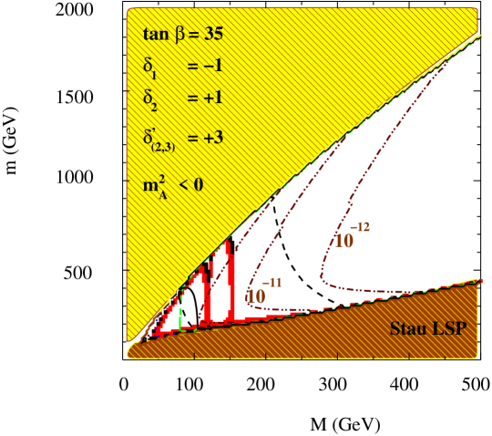
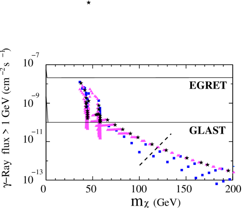
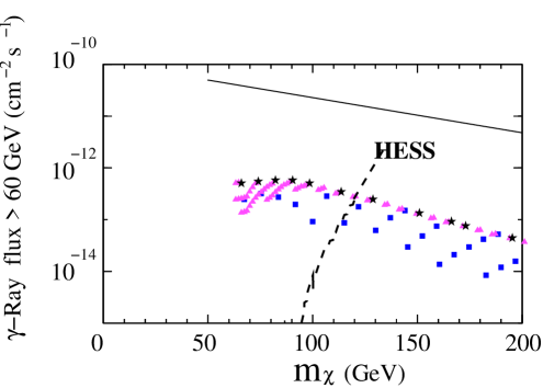
Figure 23: The same as in Fig. 3 but for $\tan\beta=$35 and the non-universal scalar and gaugino case $\delta_{2}=1,\delta_{1}=-1$, $\delta_{2}^{\prime}=\delta_{3}^{\prime}=3$. The region to the left of the solid line is excluded by $b\to s\gamma$.

         

Figure 24: The same as in Fig. 4 but for $\tan\beta=$35 and the non-universal scalar and gaugino case $\delta_{2}=1,\delta_{1}=-1$, $\delta_{2}^{\prime}=\delta_{3}^{\prime}=3$, using the same parameter space as in Fig. 24. Now, the region to the right of the dashed line corresponds to $a^{\rm SUSY}_{\mu}<7.1\times 10^{-10}$, and would be excluded by $e^{+}e^{-}$ data.

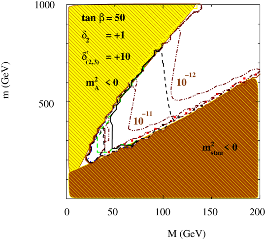
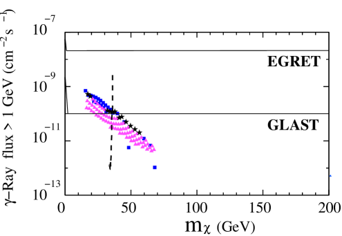
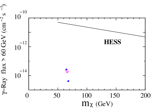
Figure 25: The same as in Fig. 3 but for $\tan\beta=$50 and the non-universal scalar and gaugino case $\delta_{2}=1,\delta_{1}=0$, $\delta_{2}^{\prime}=\delta_{3}^{\prime}=10$. The region to the left of the solid line is excluded by $b\to s\gamma$.

         

Figure 26: The same as in Fig. 4 but for $\tan\beta=50$ and the non-universal scalar and gaugino case $\delta_{2}=1,\delta_{1}=0$, $\delta_{2}^{\prime}=\delta_{3}^{\prime}=10$, using the same parameter space as in Fig. 26. Now, in the left frame, the region to the right of the dashed line corresponds to $a^{\rm SUSY}_{\mu}<7.1\times 10^{-10}$, and would be excluded by $e^{+}e^{-}$ data. In the right frame all points would be excluded by this constraint.

5 Conclusions

We have analyzed the theoretical predictions for the indirect detection of neutralino dark matter in the context of a general SUGRA theory, where both the scalar and gaugino soft supersymmetry-breaking terms can have a non-universal structure. In particular, we have computed the predictions for the gamma-ray fluxes arising from the galactic center due to neutralino annihilation, and compared it with the sensitivity of detectors.

Although the presence of non-universal scalar and gaugino masses is not able to explain the intriguing signal detected by the space-based experiment EGRET, the annihilation cross section increases significantly with respect to the universal (mSUGRA) case, producing larger gamma-ray fluxes. For example, whereas mSUGRA is not compatible for $\tan\beta<35$ with the sensitivity of another crucial projected experiment, GLAST, non-universality in the scalar sector can increase the gamma-ray fluxes about two orders of magnitude, entering in the region which will be analyzed by this experiment. For the atmospheric Cherenkov detector HESS, which has already begun operations, the situation is qualitatively similar. Of course, for larger values of $\tan\beta$ a similar increase in the gamma-ray fluxes is obtained. The above effects are mainly due to the Higgsino nature of the neutralino and/or the decrease of the CP-odd Higgs ($A$) mass in some regions of the parameter space with non-universalities.

When non-universal gauginos are considered, one can also obtain regions of the parameter space with annihilation cross sections much larger than in mSUGRA. This is also the case when it is combined with non-universal scalars, i.e. the most general case in SUGRA. In addition, in this general case, departures from the allowed parameter space obtained in the previous situations are possible. For example, neutralinos as light as $m_{\tilde{\chi}_{1}^{0}}\sim 15$ GeV, and with large fluxes can be obtained.

This general analysis can be very useful in the study of more specific cases, such as the SUGRA theories resulting at the low energy limit of string constructions. In particular, D-brane scenarios in type I string theory give rise to theories where non-universalities appear both in the scalar and gaugino sectors.

Let us finally remark that the above results have been obtained using the standard NFW density profile for our galaxy. However, we have discussed how they can easily be extended for other widely used profiles, such as Isothermal, Kravtsov et al., Navarro et al., and Moore et al. In particular, one can use Table 1 where the function $\bar{J}(\Delta\Omega)$ has been computed for the different profiles (and possible angular resolutions). This simply enters as a scaling factor in the gamma-ray fluxes. Obviously, a Moore et al. profile, which is about two orders of magnitude larger than the NFW one, would modify drastically the results concerning EGRET.

Acknowledgements

Y. Mambrini thanks E. Nezri and D.G. Cerdeño for valuable discussions and A.M. Teixeira for the help provided during this study. The work of Y. Mambrini was supported by the European Union under contract HPRN-CT-2000-00148. The work of C. Muñoz was supported in part by the Spanish DGI of the MEC under contracts BFM2003-01266 and FPA2003-04597; and the European Union under contract HPRN-CT-2000-00148.

References

- [1] For reviews, see e.g. M. Persic, P. Salucci and F. Stel, ‘The universal rotation curve of spiral galaxies: I. The dark matter connection’, Mon. Not. Roy. Astron. Soc. 281 (1996) 27 [arXiv:astro-ph/9506004]; Y. Sofue and V. Rubin, ‘Rotation curves of spiral galaxies’, [arXiv:astro-ph/0010594]; M. Roncadelli, ‘Searching for dark matter’, [arXiv:astro-ph/0307115]; P. Salucci and M. Persic, ‘Dark matter halos around galaxies’, [arXiv:astro-ph/9703027]; E. Battaner and E. Florido, ‘The rotation curve of spiral galaxies and its cosmological implications’, Fund. Cosmic Phys. 21 (2000) 1 [arXiv:astro-ph/0010475].
- [2] For a review, see W. L. Freedman, ‘Determination of cosmological parameters’, Phys. Scripta T85 (2000) 37 [arXiv:astro-ph/9905222].
- [3] WMAP Collaboration, C. L. Bennett et al., ‘First year wilkinson microwave anisotropy probe (WMAP) observations: preliminary maps and basic results’, Astrophys. J. Suppl. 148 (2003) 1 [arXiv:astro-ph/0302207]; D. N. Spergel et al., ‘First year wilkinson microwave anisotropy probe (WMAP) observations: determination of cosmological parameters’, Astrophys. J. Suppl. 148 (2003) 175 [arXiv:astro-ph/0302209]; L. Verde et al., ‘First year Wilkinson microwave anisotropy probe (WMAP) observations: parameter estimation methodology’, Astrophys. J. Suppl. 148 (2003) 195 [arXiv:astro-ph/0302218].
- [4] For a review, see e.g. J. L. Feng, K. T. Matchev, F. Wilczek, ‘Prospects for indirect detection of neutralino dark matter’, Phys. Rev. D63 (2001) 045024 [arXiv:astro-ph/0008115].
- [5] J. E. Gunn, B. W. Lee, I. Lerche, D. N. Schramm and G. Steigman, ‘Some astrophysical consequences of the existence of a heavy stable neutral lepton’, Astrophys. J. 223 (1978) 1015; F. W. Stecker, ‘The cosmic gamma-ray background from the annihilation of primordial stable neutral heavy leptons’, Astrophys. J. 223 (1978) 1032; M. Srednicki, S. Theisen and J. Silk, ‘Cosmic quarkonium: A probe of dark matter’ Phys. Rev. Lett. 56 (1986) 263, Erratum-ibid. 56 (1986) 1883; S. Rudaz, ‘Cosmic production of quarkonium?’, Phys. Rev. Lett. 56 (1986) 2128; M. S. Turner, ‘Probing the structure of the galactic halo with gamma rays produced by annihilations of weakly interacting massive particle’, Phys. Rev. D34 (1986) 34; L. Bergstrom and H. Snellman, ‘Observable monochromatic photons from cosmic photino annihilation’, Phys. Rev. D37 (1988) 3737; F. W. Stecker, Phys. Lett. B201 (1988) 529; F. W. Stecker and A. J. Tylka, ‘Spectra, fluxes and observability of gamma-rays from dark matter annihilation in the galaxy’, Astrophys. J. 343 (1989) 169; A. Bouquet, P. Salati and J. Silk, ‘Gamma-ray lines as a probe for a cold dark matter halo’, Phys. Rev. D40 (1989) 3168; S. Rudaz and F. W. Stecker, ‘On the observability of the gamma-ray line flux from dark matter annihilation’ Astrophys. J. 368 (1991) 406.
- [6] M. Urban, A. Bouquet, B. Degrange, P. Fleury, J. Kaplan, A. L. Melchior and E. Pare, ‘Searching for TeV dark matter by atmospheric Cherenkov techniques’, Phys. Lett. B293 (1992) 136 [arXiv:hep-ph/9208255]; V. S. Berezinsky, A. V. Gurevich and K. P. Zybin, ‘Distribution of dark matter in the galaxy and the lower limits for the masses of supersymmetric particles’, Phys. Lett. B294 (1992) 221; V. Berezinsky, A. Bottino and G. Mignola, ‘High-energy gamma radiation from the galactic center due to neutralino annihilation’, Phys. Lett. B325 (1994) 136 [arXiv:hep-ph/9402215].
- [7] L. Bergstrom, J. Edsjö and P. Ullio, ‘Possible indications of a clumpy dark matter halo’, Phys. Rev. D58 (1998) 083507 [arXiv:astro-ph/9804050]; L. Bergstrom, J. Edsjö, P. Gondolo and P. Ullio, ‘Clumpy neutralino dark matter’, Phys. Rev. D59 (1999) 043506 [arXiv:astro-ph/9806072].
- [8] E. Baltz, C. Briot, P. Salati, R. Taillet and J. Silk, ‘Detection of neutralino annihilation photons from external galaxies’, Phys. Rev. D61 (2000) 023514 [arXiv:astro-ph/9909112]; A. Falvard et al., ‘Supersymmetric dark matter in M31: can one see neutralino annihilation with CELESTE?’, Astropart. Phys. 20 (2004) 467; L. Pieri and E. Branchini, ‘On dark matter annihilation in the local group’, Phys. Rev. D69 (2004) 043512 [arXiv:astro-ph/0307209]; S. Peirani, R. Mohayaee and J. A. de Freitas Pacheco, ‘Indirect search for dark matter: prospects for GLAST’, arXiv:astro-ph/0401378.
- [9] P. Ullio, L. Bergstrom, J. Edsjo and C. Lacey, ‘Cosmological dark matter annihilations into gamma-rays - a closer look’, Phys. Rev. D66 (2002) 123502 [astro-ph/0207125].
- [10] L. Bergstrom, P. Ullio and J. H. Buckley, ‘Observability of gamma rays from dark matter neutralino annihilations in the Milky Way halo’, Astropart. Phys. 9 (1998) 137 [arXiv:astro-ph/9712318].
- [11] L. Bergström and P. Ullio, ‘Full one-loop calculation of neutralino annihilation into two photons’, Nucl. Phys. B504 (1997) 27 [arXiv:hep-ph/9706232]; Z. Bern P. Gondolo and M. Perelstein, ‘Neutralino annihilation into two photons’, Phys. Lett. B411 (1997) 86 [arXiv:hep-ph/9706538].
- [12] P. Ullio and L. Bergström, ‘Neutralino annihilation into a photon and a boson’, Phys. Rev. D57 (1998) 1962 [arXiv:hep-ph/9707333].
- [13] V. S. Berezinsky, A. Bottino and V. de Alfaro, ‘Is it possible to detect the gamma ray line from neutralino-neutralino annihilation?’, Phys. Lett. B274 (1992) 122.
- [14] H. U. Bengtsson, P. Salati and J. Silk, ‘Quark flavours and the -ray spectrum from halo dark matter annihilations’, Nucl. Phys., B346 (1990) 129.
- [15] G. Bertone, G. Servant and G. Sigl, ‘Indirect detection of Kaluza-Klein dark matter’, Phys. Rev. D68 (2003) 044008 [arXiv:hep-ph/0211342].
- [16] A. Cesarini, F. Fucito, A. Lionetto, A. Morselli and P. Ullio, ‘The galactic center as a dark matter gamma-ray source’, Astropart. Phys. 21 (2004) 267 [arXiv:astro-ph/0305075].
- [17] W. de Boer, M. Herold, C. Sander and V. Zhukov, ‘Indirect evidence for the supersymmetric nature of dark matter from the combined data on galactic positrons, antiprotons and gamma rays’, [arXiv:hep-ph/0309029].
- [18] D. Hooper and L.-T. Wang, ‘Direct and indirect detection of neutralino dark matter in selected supersymmetry breaking scenarios’, Phys. Rev. D69 (2004) 035001 [arXiv:hep-ph/0309036].
- [19] H. Baer, A. Belyaev, T.Krupovnickas and J. O’Farrill, ‘Indirect, direct and collider detection of neutralino dark matter’, [arXiv:hep-ph/0405210].
- [20] D. Hooper and B. Dingus, ‘Improving the angular resolution of EGRET and new limits on supersymmetric dark matter near the galactic center’, [arXiv:astro-ph/0212509]
- [21] A. Bottino, F. Donato, N. Fornengo and S. Scopel, ‘Indirect signals from light neutralinos in supersymmetric models without gaugino mass unification’, [arXiv:hep-ph/0401186].
- [22] D. Elsasser and K. Mannheim, ‘Supersymmetric dark matter and the extragalactic gamma ray background’, [arXiv:astro-ph/0405325].
- [23] P. Binetruy, A. Birkedal-Hansen, Y. Mambrini and B.D. Nelson, ‘Phenomenological aspects of heterotic orbifold models at one loop,’ [arXiv:hep-ph/0308047].
- [24] G. Bertone, P. Binetruy, Y. Mambrini and E. Nezri, ‘Annihilation radiation of dark matter in heterotic orbifold models’, [arXiv:hep-ph/0406083].
- [25] EGRET Collaboration, S. D. Hunger et al., ‘EGRET observations of the diffuse gamma-ray emission from the galactic plane’, Astrophys. J. 481 (1997) 205; H. A. Mayer-Hasselwander et al., ‘High-Energy Gamma-Ray Emission from the Galactic Center’ Astron. & Astrophys. 335 (1998) 161.
- [26] I. Busching, M. Pohl and R. Schlickeiser, ‘Excess GeV radiation and cosmic ray origin’, Astron. & Astrophys. 377 (2001) 1056 [arXiv:astro-ph/0108321]; A. D. Erlykin and A. W. Wolfendale, ‘Supernova remnants and the origin of cosmic radiation: evidence from low-energy gamma-rays’, J. Phys. G28 (2002) 2329; F. A. Aharonian and A. M. Atoyan, ‘Broad-band diffuse gamma-ray emission of the galactic disk’, Astron. & Astrophys. 362 (2000) 937 [arXiv:astro-ph/0009009]; A. W. Strong, I. V. Moskalenko and O. Reimer, ‘Diffuse galactic continuum gamma rays. A model compatible with EGRET data and cosmic-ray measurements’, [arXiv:astro-ph/0406254].
- [27] N. Gehrels, P. Michelson, ‘GLAST: the next generation high-energy gamma-ray astronomy mission’, Astropart. Phys. 11 (1999) 277; See also the web page http://www-glast.stanford.edu
- [28] HESS Collaboration, J. A. Hinton et al., ‘The status of the HESS project’, New Astron. Rev. 48 (2004) 331 [arXiv:astro-ph/0403052].
- [29] For a review, see A. Brignole, L. E. Ibañez and C. Muñoz, ‘Soft supersymmetry-breaking terms from supergravity and superstring models’, in the book ’Perspectives on supersymmetry’, Ed. G. Kane, World Scientific (1998) 125 [arXiv:hep-ph/9707209].
- [30] L. E. Ibañez, C. Muñoz and S. Rigolin, ‘Aspects of type I string phenomenology’, Nucl. Phys. 553 (1999) 43 [arXiv:hep-ph/9812397].
- [31] Y. Mambrini and C. Muñoz, in preparation.
- [32] F. Eisenhauer et al., ‘A geometric determination of the distance to the galactic center’, Astrophys. J. 597 (2003) L121 [arXiv:astro-ph/0306220].
- [33] L. Hernquist, ‘An analitical model for spherical galaxies and bulges’, Astrophys. J. 356 (1990) 359.
- [34] S.H. Hansen, ‘Dark matter density profiles from the Jeans equation’, Mon. Not. Roy. Astron. Soc. 352 (2004) L41 [arXiv:astro-ph/0405371].
- [35] J. F. Navarro, C. S. Frenk and S. D. M. White, ‘The structure of cold dark matter halos’, Astrophys. J. 462 (1996) 563 [arXiv:astro-ph/9508025].
- [36] B. Moore, T. Quinn, F. Governato, J. Stadel and G. Lake, ‘Cold collapse and the core catastrophe’, Mon. Not. Roy. Astron. Soc. 310 (1999) 1147 [arXiv:astro-ph/9903164].
- [37] A. V. Kravtsov, A. A. Klypin, J. S. Bullock and J. R. Primack, ‘The cores of dark matter dominated galaxies: theory vs. observations’, Astrophys. J. 502 (1998) 48 [arXiv:astro-ph/9708176].
- [38] J. F. Navarro et al., ‘The inner structure of CDM halos III: universality and asymptotic slopes’, Mon. Not. Roy. Astron. Soc. 349 (2004) 1039 [arXiv:astro-ph/0311231].
- [39] R. Schodel et al., ‘A star in a 15.2-year orbit around the supermassive black hole at the centre of the Milky Way’, Nature 419 (2002) 694 [arXiv:astro-ph/0210426].
- [40] P. Gondolo and J. Silk, ‘Dark matter annihilation at the galactic center’, Phys. Rev. Lett. 83 (1999) 1719 [arXiv:astro-ph/9906391].
- [41] G. Bertone, G. Sigl and J. Silk, ‘Annihilation radiation from a dark matter spike at the galactic centre’, Mon. Not. Roy. Astron. Soc. 337 (2002) 98 [arXiv:astro-ph/0203488].
- [42] L. Bergstrom, J. Edsjo and P. Ullio, ‘Spectral gamma-ray signatures of cosmological dark matter annihilations’, Phys. Rev. Lett. 87 (2001) 251301 [arXiv:astro-ph/0105048].
- [43] T. Sjostrand et al., ‘High-Energy-Physics Event Generation with PYTHIA 6.1’, Comput. Phys. Commun. 135 (2001) 238 [arXiv:hep-ph/0010017].
- [44] R.G. Roberts and L. Roszkowski, ‘Implications for minimal supersymmetry from grand unification and the neutralino relic abundance’, Phys. Lett. B309 (1993) 329 [arXiv:hep-ph/9301267]; G. Kane, C.F. Kolda, L. Roszkowski and J.D. Wells, ‘Study of constrained minimal supersymmetry’, Phys. Rev. D49 (1994) 6173 [arXiv:hep-ph/9312272].
- [45] See also, P. Nath and R. Arnowitt, ‘Top quark mass and Higgs mass limits in the standard supergravity unification’, Phys. Lett. B289 (1992) 368.
- [46] P. Gondolo, J. Edsjo, L. Bergstrom, P. Ullio and E. A. Baltz, ‘DarkSUSY - A numerical package for dark matter calculations in the MSSM’, [arXiv:astro-ph/0012234].
- [47] A. Djouadi, J. L. Kneur and G. Moultaka, ‘SuSpect: a Fortran code for the supersymmetric and Higgs particle spectrum in the MSSM’, [arXiv:hep-ph/0211331]; See also the web page http://www.lpm.univ-montp2.fr:6714/~kneur/suspect.html
- [48] G. Belanger, F. Boudjema, A. Pukhov and A. Semenov, ‘micrOMEGAs: a program for calculating the relic density in the MSSM’, Comput. Phys. Commun. 149 (2002) 103 [arXiv:hep-ph/0112278]; ‘MicrOMEGAs: recent developments’, arXiv:hep-ph/0210327; G. Belanger, ‘micrOMEGAs and the relic density in the MSSM’, [arXiv:hep-ph/0210350]; See also the web page http://wwwlapp.in2p3.fr/lapth/micromegas
- [49] P. Gondolo, J. Edsjo, P. Ullio, L. Bergstrom, M. Schelke and E. A. Baltz, ‘DarkSUSY: Computing supersymmetric dark matter properties numerically’, [arXiv:astro-ph/0406204]; See also the web page http://www.physto.se/ edsjo/darksusy
- [50] Muon g-2 Collaboration, G. W. Bennett et al., ‘Measurement of the negative muon anomalous magnetic moment to 0.7-ppm’, Phys. Rev. Lett. 92 (2004) 161802 [arXiv:hep-ex/0401008].
- [51] M. Davier, S. Eidelman, A. Höcker and Z. Zhang, ‘Updated estimate of the muon magnetic moment using revised results from annihilation’, Eur. Phys. J. C 31 (2003) 503 [arXiv:hep-ph/0308213]; K. Hagiwara, A. D. Martin, D. Nomura and T. Teubner, ‘Predictions for of the muon and ’, Phys. Rev. D69 (2004) 093003 [arXiv:hep-ph/0312250]; J. F. de Trocóniz and F. J. Ynduráin, ‘The hadronic contributions to the anomalous magnetic moment of the muon’, [arXiv:hep-ph/0402285].
- [52] CLEO Collaboration, S. Chen et al., ‘Branching fraction and photon energy spectrum for ’, Phys. Rev. Lett. 87 (2001) 251807. [arXiv:hep-ex/0108032]
- [53] BELLE Collaboration, H. Tajima, ‘Belle B physics results’, Int. J. Mod. Phys. A17 (2002) 2967 [arXiv:hep-ex/0111037].
- [54] D. G. Cerdeño, E. Gabrielli, M. E. Gomez, and C. Muñoz, ‘Neutralino nucleon cross section and charge and colour breaking constraints’, J. High Energy Phys. 06 (2003) 030 [arXiv:hep-ph/0304115].
- [55] A. Birkedal-Hansen and B. D. Nelson, ‘Relic neutralino densities and detection rates with nonuniversal gaugino masses,’ Phys. Rev. D67 (2003) 095006 [arXiv:hep-ph/0211071]; A. Birkedal-Hansen and B. D. Nelson, ‘The role of Wino content in neutralino dark matter,’ Phys. Rev. D64 (2001) 015008 [arXiv:hep-ph/0102075]; V. Bertin, E. Nezri and J. Orloff, ‘Neutralino dark matter beyond CMSSM universality,’ J. High Energy Phys. 02 (2003) 046 [arXiv:hep-ph/0210034].
- [56] D. G. Cerdeño and C. Muñoz, ‘Neutralino dark matter in supergravity theories with non-universal scalar and gaugino masses’, J. High Energy Phys. 10 (2004) 015 [arXiv:hep-ph/0405057].