DO-TH-04/08
July 2004

The 2PI finite temperature effective potential of the O(N) linear sigma model in 1+1 dimensions at next-to-leading order in 1/N

Jürgen Baacke    and    Stefan Michalski

Institut für Physik, Universität Dortmund
D–44221 Dortmund, Germany

We study the $O(N)$ linear sigma model in 1+1 dimensions by using the 2PI formalism of Cornwall, Jackiw and Tomboulis in order to evaluate the effective potential at finite temperature. At next-to-leading order in a $1/N$ expansion one has to include the sums over “necklace”’ and generalized “sunset” diagrams. We find that — in contrast to the Hartree approximation — there is no spontaneous symmetry breaking in this approximation, as to be expected for the exact theory. The effective potential becomes convex throughout for all parameter sets which include $N=4,10,100$, couplings $\lambda=0.1,0.5$ and temperatures between $0.3$ and $1$ (in arbitrary units). The Green’s functions obtained by solving the Schwinger-Dyson equations are enhanced in the infrared region. We also compare the effective potential as a function of the external field $\phi$ with those obtained in the 1PI and 2PPI expansions.

1 Introduction

The $O(N)$ linear sigma model at finite temperature has a long-standing history, in particular as a basic model for a quantum field theory with spontaneous symmetry breaking [1, 2, 3, 4]. Early investigations beyond the classical level have been based on including one-loop quantum and thermal corrections. These studies have been centered around the discussion of the one-loop effective potential $V_{\rm eff}(\phi)$ where $\phi$ is the mean value of the quantum field $\Phi$, in a sense being defined more precisely by the effective action formalism, summing up one-particle irreducible (1PI) graphs. A next class of approximations include bubble resummations, usually obtained from the 1PI formalism by introducing an auxiliary field. Within such a framework the effective potential has been computed to leading [2, 3, 5] and next-to-leading order (NLO) of a $1/N$ expansion [6]. At leading order in $1/N$ one does not find spontaneous symmetry breaking in $1+1$ dimensions, while in $3+1$ dimensions the effective potential is flat for $|\vec{\phi}|<v$ [4] . At next-to leading order there is no spontaneous symmetry breaking in $1+1$ dimensions either. These results correctly reproduce a general property of theories in $1+1$ dimensions, where spontaneous symmetry breaking is prevented by the non-existence of Goldstone bosons [7].

Another approximation including some nonleading terms of a $1/N$ expansion is the Hartree approximation. It is usually motivated by a self-consistency of one-loop quantum corrections. It has been studied in $3+1$ dimensions by various authors, in thermal equilibrium [8, 9, 10, 11, 12], and out-of-equilibrium [13]. The model with spontaneous symmetry breaking is found to have a phase transition of first order towards the symmetric phase at high temperature. In $1+1$ dimensions the Hartree approximation displays spontaneous symmetry breaking and symmetry restoration as in $3+1$ dimensions, an obviously unphysical feature.

If one wants to go beyond the large-$N$ and Hartree approximations there is a variety of choices. One of those is the use of the two-particle irreducible (2PI) formalism of Cornwall, Jackiw and Tomboulis (CJT) [14] within which one may include higher loop corrections, higher orders in $1/N$ etc., as in a 1PI expansion. But furthermore it becomes necessary to solve Schwinger-Dyson equations for the propagators in order to sum up certain classes of Feynman graphs. Apart from the fact that this may be technically demanding, there still is the obstacle that for $3+1$ dimensions renormalization has been discussed up to now only for vanishing external fields [15, 16, 17, 18]; this obstructs the discussion of spontaneous symmetry breaking, which here is our main interest. As here we discuss the model in $1+1$ dimensions, the problem of renormalization does not arise and explicit numerical computations can be performed. This is indeed the main subject of this publication.

A technically less demanding approach is the so-called two-particle point-irreducible (2PPI) resummation introduced by Coppens and Verschelde [19, 20]. Here, instead of treating the Green’s functions as variational parameters, one just introduces variational masses like in the Hartree approximation. This implies that the resummation is only over local insertions, the 2-particle point-reducible graphs, i.e., graphs that fall apart if two lines meeting at the same point (the 2PPR point) are cut. This approach is identical to the Hartree approximation if only one-loop 2PPI graphs are included. For this formalism renormalization has been fully discussed [21]; symmetry restoration at finite temperature has been investigated in $3+1$ dimensions in an approximation including the sunset diagram, for the case $N=1$ [22] and for the $O(N)$ model with arbitrary $N$ [23].

The 2PI formalism has the advantage that at a given order of the loop expansion it resums a larger class of Feynman diagrams than the 2PPI or Root’s auxiliary field scheme. From a variational point of view it allows for a more “flexible” propagator whose self-energy insertions are nonlocal in space-time and thereby become momentum dependent.

It is the purpose of the present work to study the 2PI formalism at next-to-leading order of the $1/N$ expansion, an approximation usually denoted as 2PI-NLO for short. For the $O(N)$ model the next-to-leading order 1PI diagrams have been identified in the work of Root [6] using an auxiliary field method. They are depicted in Figs. 1 and 8 in a way that graphically differs from Root’s presentation. The 2PI-NLO diagrams are obtained by omitting those which are two particle reducible, they have been discussed in Refs. [24, 25]. The sums over all “necklace” (cf. Fig.1) and “generalized sunset” (cf. Fig. 2) diagrams can be done in closed form.

We have evaluated the effective potential at finite temperature in the 2PI-NLO scheme by solving the Schwinger-Dyson gap equations. For comparison we will also show results obtained in the other schemes introduced above.

The consideration of $\Phi^{4}$ theory in $1+1$ dimensions has recently received some interest in the context of nonequilibrium dynamics [24, 26, 27, 28, 29]. A comparison [28, 30] of various approximations for the $O(1)$ model, i.e., a model with a simple double-well potential, has displayed some still not well-understood features. The $O(1)$ model has thermal kink transitions [31, 32, 33, 34] that lead to a symmetric phase in the exact theory. These are out of reach within a perturbative treatment in thermal equilibrium, whereas they may play (or seem to play) a non-perturbative rôle in nonequilibrium physics even in the approximations considered here. Our present calculations are not directly relevant to this case. However, the comparison of the various schemes for $N>1$ should be of interest as well, both in equilibrium and out of equilibrium. Here we provide the equilibrium computations, in expectation of their nonequilibrium counterparts.

The plan of the paper is as follows: in Section 2 we present the general formulation of the model and of the 2PI formalism at NLO-$1/N$. We also present all the formulae used in computing the finite-temperature effective potential in the NLO-$1/N$ approximation. This discussion includes the Hartree approximation. The analogous derivations for the 2PPI and 1PI (Root) scheme are presented in Appendix A and B. In Section 3 we discuss our numerical results. We end with some conclusions and an outlook in Section 4.

2 Basic equations

The Lagrange density of the linear sigma is given by

$${\cal L}=\frac{1}{2}\,\partial_{\mu}\vec{\Phi}\cdot\partial^{\mu}\vec{\Phi}-\frac{\lambda}{4N}\left(\vec{\Phi}^{2}-Nv^{2}\right)^{2}\;.$$ (2.1)

The 2PI effective action formalism introduces two variational functions: an external field $\phi(x)$ and a Green’s function ${\cal G}(x,x^{\prime})$, which arise as Legendre conjugate variables related to a local source term $J(x)\Phi(x)$ and a bilocal source term $K(x,x^{\prime})\Phi(x)\Phi(x^{\prime})$. Assuming that the expectation value of $\vec{\Phi}^{2}$ will scale as $N$ we introduce the external field $\phi$ with a scale factor $\sqrt{N}$, i.e., $\langle\Phi\rangle=\sqrt{N}\phi$. We then obtain the classical potential

$$V_{\rm class}(\phi)=\frac{\lambda}{4N}\left(N\phi^{2}-Nv^{2}\right)^{2}=N\frac{\lambda}{4}\left(\phi^{2}-v^{2}\right)^{2}\;.$$ (2.2)

The one-loop part of the effective action is given by

$$\Gamma_{\rm 1-loop}[\phi,\mathcal{G}]=\frac{i}{2}{\rm Tr}\ln{\cal G}^{-1}/{\cal G}_{0}^{-1}+\frac{1}{2}{\rm Tr}\left[i{\cal D}^{-1}{\cal G}-1\right]\;.$$ (2.3)

Here ${\cal G}$, ${\cal G}_{0}$ and ${\cal D}$ are matrices. If we separate the fields in a basis parallel and orthogonal to the direction $\hat{n}$ of the classical field $(\vec{\Phi})_{\rm cl}=\sqrt{N}\vec{n}\phi$ these matrices become diagonal, with one entry for the parallel component and $(N-1)$ identical entries for the orthogonal ones. We denote them as $\sigma$ and $\pi$ in reference to the linear sigma model, which presents one of the possible applications. With this notation we have

$$i{\cal D}_{j}^{-1}=-\partial_{\mu}\partial^{\mu}-\lambda(f_{j}\phi^{2}-v^{2})\;.$$ (2.4)

This is the Klein-Gordon operator in the external field; $f_{j}=3$ for $j=\sigma$ and $f_{j}=1$ for $j=\pi$. We have normalized the Green’s functions ${\cal G}_{j}$ with respect to free Green’s functions

$${\cal G}_{j,0}^{-1}=-\partial_{\mu}\partial^{\mu}-m_{j,0}^{2}\;.$$ (2.5)

The higher terms in the effective action are all two-particle irreducible vacuum Feynman graphs with external lines $\sqrt{N}\phi(x)$ and with Green’s function ${\cal G}$ as internal lines.

In the following we will consider the system at finite temperature. So we perform the Wick rotation and replace the integration over the Euclidean $p^{0}$ by the summation over the Matsubara frequencies $p^{0}_{n}=\omega_{n}=2n\pi k_{B}T$. Furthermore we consider the effective potential instead of the effective action. Then the one-loop term for one species, $j=\sigma$ or $j=\pi$ takes the form

$$V_{\rm 1-loop,j} = \frac{1}{2}T\sum_{m=-\infty}^{\infty}\int_{-\infty}^{\infty}\frac{dq}{2\pi}\left\{\ln\frac{q^{2}+\omega_{m}^{2}+m_{j,0}^{2}+\Sigma_{j}(\omega_{m},q)}{q^{2}+\omega_{m}^{2}+m_{j,0}^{2}}\right.$$

$$\left.-\left[m_{j,0}^{2}+\Sigma_{j}(\omega_{m},q)-\lambda(f_{j}\phi^{2}-v^{2})\right]{\cal G}_{j}(\omega_{m},q)\right\}\;.$$

Here

$${\cal G}_{j,0}^{-1}(\omega_{n},p)=p^{2}+\omega_{n}^{2}+m_{j,0}^{2}$$ (2.7)

is the reference Green’s function, and $\Sigma_{j}(\omega_{n},p)$ is defined as

$$\Sigma_{j}(\omega_{n},p)={\cal G}_{j}^{-1}(\omega_{n},p)-{\cal G}_{j,0}^{-1}(\omega_{n},p)\;.$$ (2.8)

The choice of $m_{0j}$ only introduces an additive, though temperature dependent, constant to the effective potential. An obvious choice would be to use the bare physical masses, but this would imply $m_{\pi 0}^{2}=0$, leading immediately to infrared singularities. As we anticipate that the symmetry may not be broken in the NLO-$1/N$ approximation, we prefer a symmetric choice: $m_{j0}^{2}=\lambda v^{2}$ for both $j=\sigma$ and $j=\pi$.

The one-loop potential is divergent. The asymptotic behavior of the integrand is

$$\left\{\cdots\right\}\simeq-\frac{m_{j0}^{2}-\lambda(f_{j}\phi^{2}-v^{2})}{q^{2}+\omega_{n}^{2}+m_{j,0}^{2}}\;.$$ (2.9)

So the integral of the one-loop effective action can be regulated by subtracting this term and by adding it in regularized form. We have

$$V_{\rm 1-loop,j} = \frac{1}{2}T\sum_{m=-\infty}^{\infty}\int_{-\infty}^{\infty}\frac{dq}{2\pi}\left\{\ln\frac{q^{2}+\omega_{m}^{2}+m_{j,0}^{2}+\Sigma_{j}(\omega_{m},q)}{q^{2}+\omega_{m}^{2}+m_{j,0}^{2}}\right.$$ (2.10)

$$\left.-\left[m_{j,0}^{2}+\Sigma_{j}(\omega_{m},q)-\lambda(f_{j}\phi^{2}-v^{2})\right]{\cal G}_{j}(\omega_{m},q)\right.$$

$$\left.+\frac{m_{j0}^{2}-\lambda(f_{j}\phi^{2}-v^{2})}{q^{2}+\omega_{n}^{2}+m_{j,0}^{2}}\right\}$$

$$-\left[m_{j0}^{2}-\lambda(f_{j}\phi^{2}-v^{2})\right]{\cal B}_{j0}$$

where ${\cal B}_{j}$ are the bubble diagrams which we regularize dimensionally as

$${\cal B}_{j,0} = T\sum_{m=-\infty}^{\infty}\int\frac{dq^{(1-\epsilon)}}{(2\pi)^{(1-\epsilon)}}{\cal G}_{j,0}(\omega_{m},q)$$ (2.11)

$$= \frac{1}{4\pi}\left[\frac{2}{\epsilon}-\gamma_{E}+\ln 4\pi-\ln\frac{m_{j,0}^{2}}{\mu_{j}^{2}}\right]+\int\frac{dq}{2\pi\omega}\,\frac{1}{\exp\beta\sqrt{q^{2}+m_{j,0}^{2}}-1}\;.$$

We define their finite part ${\cal B}_{j,0,\rm fin}$ using the $\overline{\rm MS}$ prescription, leaving out the terms $2/\epsilon-\gamma_{E}+\ln(4\pi)$. Then the renormalized bubble diagrams become

$${\cal B}_{j}=T\sum_{m=-\infty}^{\infty}\int\frac{dp}{2\pi}\left[{\cal G}_{j}(\omega_{n},p)-{\cal G}_{j,0}(\omega_{n},p)\right]+{\cal B}_{j,0,\rm fin}\;.$$ (2.12)

with

$${\cal B}_{j,0,\rm fin}=\frac{-1}{4\pi}\ln\frac{m_{j,0}^{2}}{\mu_{j}^{2}}+\int\frac{dq}{2\pi\omega}\,\frac{1}{\exp\beta\sqrt{q^{2}+m_{j,0}^{2}}-1}\;.$$ (2.13)

For the renormalization scale we choose $\mu_{j}^{2}=m_{j0}^{2}=\lambda v^{2}$. In $1+1$ dimensions the theory is renormalized if the Hamiltonian is normal-ordered. This is not a unique prescription as the normal-ordering may be done with respect to different masses of the bare quanta [35, 36]. A shift in these masses introduces a redefinition of the vacuum expectation value $v$, or of the mass parameter in the symmetric theory, as the change in normal ordering of the $\phi^{4}$ term introduces a term quadratic in the fields. In the present context we have to take the renormalization scale identical for the $\sigma$ and $\pi$ modes as otherwise we break the symmetry explicitly. Our convention corresponds to normal-ordering with respect to bare quanta of mass $\lambda v^{2}$.

With these preliminaries the total one-loop effective potential is given by

$$V_{{\rm 1-loop}}=V_{{\rm 1-loop},\sigma}+(N-1)V_{{\rm 1-loop},\pi}\;.$$ (2.14)

The first nontrivial term is the double-bubble diagram. As we consider here leading order and next-to-leading order contributions we have to calculate this diagram with the exact combinatorial factors for $O(N)$. It takes the form

$$V_{\rm db} = \frac{\lambda}{4N}\left\{[\mathcal{B}_{\sigma}+(N-1)\mathcal{B}_{\pi}]^{2}+2\,[\mathcal{B}_{\sigma}+(N-1)\mathcal{B}_{\pi}]\right\}$$ (2.15)

$$= \frac{\lambda}{4N}\left[(N^{2}-1){\cal B}_{\pi}^{2}+2(N-1){\cal B}_{\sigma}{\cal B}_{\pi}+3{\cal B}_{\sigma}^{2}\right]\;.$$

If only these two contributions are considered, we obtain the Hartree approximation, or daisy and super-daisy resummation. In writing down this contribution we have replaced the divergent bubbles subdiagrams by the finite ones. This requires mass and vacuum energy counterterms which here are fixed by the minimal subtraction prescription which eventually may be replaced by a precise renormalization condition.

From

$$V_{\rm{Hartree}}=V_{\rm 1-loop}+V_{\rm db}$$ (2.16)

we obtain the gap equations

$$\Sigma^{H}_{\sigma}(\omega_{n},p) = -m_{\sigma 0}^{2}+\lambda(3\phi^{2}-v^{2})+\frac{\lambda}{N}\left[3{\cal B}_{\sigma}+(N-1){\cal B}_{\pi}\right]$$ (2.17a)

$$\Sigma^{H}_{\pi}(\omega_{n},p) = -m_{\pi 0}^{2}+\lambda(\phi^{2}-v^{2})+\frac{\lambda}{N}\left[{\cal B}_{\sigma}+(N+1){\cal B}_{\pi}\right]$$ (2.17b)

When taking the functional derivative with respect to ${\cal G}_{\pi}$ we will, here and below, consider each pion “individually”, disregarding factors $(N-1)$ which would cancel in the gap equation. In this way the second equation is obtained directly, and the sigma and “each” pion field are treated on the same footing.

The large-$N$ limit is obtained by omitting the sigma contribution entirely. Then the first of the gap equations is omitted as well, and the second one only contains the pion bubble with $N/(N-1)$ replaced by unity.

The condition for a nontrivial extremum with respect to $\phi$ becomes

$${\cal R}(\phi)=\frac{1}{N\phi}\frac{\partial V_{\rm{eff}}^{H}}{\partial\phi}=\lambda(\phi^{2}+{\cal B}-v^{2})=0$$ (2.18)

with the compound bubble diagram

$${\cal B}=\frac{\partial\left[3V_{\rm{1-loop},\sigma}+(N-1)V_{\rm{1-loop},\pi}\right]}{\partial\phi}=\frac{1}{N}\left[3{\cal B}_{\sigma}+(N-1){\cal B}_{\pi}\right]\;.$$ (2.19)

Again in the large-$N$ limit the sigma contribution is neglected and the prefactor $N/(N-1)$ of the pion bubble is replaced by unity. To next-to-leading order in a $1/N$ expansion one has, in the absence of external fields, to sum over all diagrams which are traces of powers of the fish diagram, the so-called necklace diagrams, shown in Fig. 1. In order to go beyond the leading order we define several diagrams: We denote the fish diagrams by ${\cal F}_{j}(\omega_{n},p)$; explicitly

$${\cal F}_{j}(\omega_{n},p)=T\sum_{m=-\infty}^{\infty}\int\frac{dq}{2\pi}\ {\cal G}_{j}(\omega_{m},q){\cal G}_{j}(\omega_{n}-\omega_{m},p-q)$$ (2.20)

and denote by ${\cal F}(\omega_{n},p)$ the “average” fish

$${\cal F}(\omega_{n},p)=\frac{1}{N}\left[(N-1){\cal F}_{\pi}(\omega_{n},p)+{\cal F}_{\sigma}(\omega_{n},p)\right]\;.$$ (2.21)

The sum over the necklace without external fields, see Fig. 1, is then given by

$${\cal N}=\frac{1}{2}T\sum_{m=-\infty}^{\infty}\int\frac{dq}{2\pi}\left\{\ln[1+\lambda{\cal F}(\omega_{m},q)]-\lambda{\cal F}(\omega_{m},q)\right\}\;.$$ (2.22)

The subtraction of $\lambda{\cal F}(\omega_{m},p)$ accounts for the fact that we have already included the double-bubble diagrams. In the symmetric theory where the $\sigma$ and $\pi$ contributions are equal, the factor $N$ cancels, so this expression is of order $N^{0}$ which is NLO.

The same order in $1/N$ is achieved by replacing one of the $\sigma$ lines of the necklace by $N\phi^{2}$. We will call this class of graphs “generalized sunsets”, see Fig. 2 for a graphical depiction. We introduce the derivative

$$\frac{\delta{\cal N}}{\delta{\cal G}_{j}}(\omega_{n},p)=\frac{\lambda}{N}T\sum_{m=-\infty}^{\infty}\int\frac{dq}{2\pi}\frac{-\lambda{\cal F}(\omega_{m},q)}{1+\lambda{\cal F}(\omega_{m},q)}\ {\cal G}_{j}(\omega_{n}-\omega_{m},p-q)\;.$$ (2.23)

Note that the factor $\lambda/N$ arises from the derivative of the expression $\lambda{\cal F}(\omega_{n},p)$ with respect to ${\cal G}_{j}$. In terms of $\delta{\cal N}/\delta{\cal G}_{\sigma}$ we obtain for the generalized sunset diagram, or sum over necklace diagrams with two external lines

$${\cal S}=N\phi^{2}\frac{\delta{\cal N}}{\delta{\cal G}_{\sigma}}(0,0)=\lambda\phi^{2}T\sum_{m=-\infty}^{\infty}\int\frac{dq}{2\pi}\frac{-\lambda{\cal F}(\omega_{m},q)}{1+\lambda{\cal F}(\omega_{m},q)}{\cal G}_{j}(\omega_{m},q)\;.$$ (2.24)

The functional derivative contains a factor $1/N$ so that this expression is of order $N^{0}$. With these definitions the 2PI effective potential up to NLO becomes

$$V_{\rm eff}=V_{\rm class}+V_{\rm 1-loop}+V_{\rm db}+{\cal S}+{\cal N}$$ (2.25)

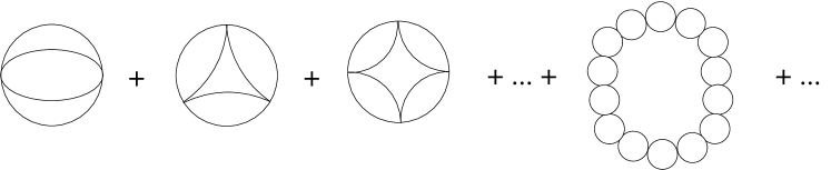
Figure 1: Resummation of necklace graphs.

Figure 2: Generalized sunset graphs.

In order to write down the gap equations we need to introduce a further functional derivative

$$\frac{\delta{\cal S}}{\delta{\cal G}_{j}}(\omega_{n},p)=N\phi^{2}\frac{\delta}{\delta{\cal G}_{j}(\omega_{n},p)}\left[\frac{\delta{\cal N}}{\delta{\cal G}_{\sigma}}(0,0)\right]\;.$$ (2.26)

Explicitly it is given by

$$\frac{\delta{\cal S}}{\delta{\cal G}_{j}}(\omega_{n},p)=\frac{\lambda^{2}}{N}\phi^{2}\,T\int\frac{dq}{2\pi}\frac{-1}{[1+\lambda{\cal F}(\omega_{m},q)]^{2}}{\cal G}_{\sigma}(\omega_{m},q){\cal G}_{j}(\omega_{n}-\omega_{m},p-q)$$

$$+\lambda\phi^{2}\delta_{j\sigma}\frac{-\lambda{\cal F}(\omega_{n},p)}{1+\lambda{\cal F}(\omega_{n},p)}\;.$$ (2.27)

With these definitions the gap equations become

$$\Sigma_{\sigma}(\omega_{n},p) = -m_{\sigma 0}^{2}+\lambda(3\phi^{2}-v^{2})+\frac{\lambda}{N}\left[(N-1){\cal B}_{\pi}+3{\cal B}_{\sigma}\right]$$ (2.28a)

$$+\frac{\delta{\cal N}}{\delta{\cal G}_{\sigma}}(\omega_{n},p)+\frac{\delta{\cal S}}{\delta{\cal G}_{\sigma}}(\omega_{n},p)$$

$$\Sigma_{\pi}(\omega_{n},p) = -m_{\pi 0}^{2}+\lambda(\phi^{2}-v^{2})+\frac{\lambda}{N}\left[(N+1){\cal B}_{\pi}+{\cal B}_{\sigma}\right]$$ (2.28b)

$$+\frac{\delta{\cal N}}{\delta{\cal G}_{\pi}}(\omega_{n},p)+\frac{\delta{\cal S}}{\delta{\cal G}_{\pi}}(\omega_{n},p)$$

All expressions in these equations have been given explicitly above. Finally for the partial derivative of $V_{\rm eff}$ with respect to $\phi$ we find

$${\cal R}(\phi)=\frac{1}{N\phi}\frac{\partial V_{\rm{eff}}}{\partial\phi}=\lambda(\phi^{2}+{\cal B}-v^{2})+2\lambda\frac{\delta{\cal N}}{\delta{\cal G}_{\sigma}}(0,0)$$ (2.29)

We have performed the computations for the 2PPI scheme of Verschelde and Coppens as well, including necklace and generalized sunset diagrams. The formulae and their derivation are rather similar to those of the 2PI scheme. They are given in Appendix A.

3 Numerics and Results

The equations of the previous section are easily incorporated into a computer code; we solve the gap equations by iteration. The range of momenta and Matsubara frequencies was restricted to values smaller than $15-20$, far above the relevant mass scales. All numerical integrals and summations are ultraviolet finite by the regularization presented in the previous section.

For the first step at fixed $N,v,\lambda,T$ and $\phi$ we start with ${\cal G}_{j}={\cal G}_{j0}$. The iteration is monitored by the values of the average bubble diagram

$$\overline{{\cal B}}=\left[(N-1){\cal B}_{\pi}+{\cal B}_{\sigma}\right]/N\;.$$ (3.30)

If the relative change of this global quantity has become smaller than $10^{-8}$ the iteration is considered to have reached the solution.

For temperatures of the order of $v$ this procedure converges well. Problems arise if the temperature is low, typically less then $v/5$ and for $\phi$ typically less than $v/2$. In these regions the pion propagator becomes large at small $(\omega_{n},p)$ obviously due to a pion pole approaching $p^{2}=0$ from negative (Minkowskian) $p^{2}$. This situation is close to an infrared divergence, and small changes of the pion Green’s function result in large changes of the various integrals. One can extend the domain of convergence by using an underrelaxation, defining the $n$th step of the iteration of Eqs. (2.28) by taking the result $\Sigma^{(n-1)}_{j}$ of the previous step multiplied by a factor of $\alpha$ plus the right hand sides of these equations multiplied by $(1-\alpha)$. We have chosen $\alpha$ typically between $.5$ and $.95$.

In order to be sure of the consistency of our search for extrema, both in the analytic formulas and in the numerical computations we have not only computed the results for $\partial V_{\rm eff}[\phi,\bar{\cal G}_{j}]/\partial\phi$ but also the potential $V_{\rm eff}[\phi,\bar{\cal G}_{j}]$ itself. Here in both cases the Green’s functions ${\cal G}_{j}$ were the solutions $\bar{\cal G}_{j}$ of the gap equations; so both $V_{\rm eff}$ and $\partial V_{\rm eff}/\partial\phi$ are evaluated at $\delta V_{\rm eff}/\delta{\cal G}=0$ and the extrema of the potential $V_{\rm eff}[\phi,\bar{\cal G}_{j}]$ should coincide with the zeros of $\partial V_{\rm eff}[\phi,\bar{\cal G}_{j}]/\partial\phi$. For the computations in the 2PI scheme we do not find any nontrivial minima, so all we check here is that ${\cal R}(\phi)$ has no zeros. For the Hartree approximation and for the 2PPI scheme, the extrema of the potential and the zeros of ${\cal R}(\phi)$ agree within the avalailable accuracy.

In Figs. 3 and 4 we show the temperature dependence of the 2PI effective potential, for $N=4$ and $\lambda=0.5$ and $\lambda=0.1$. The effective potential shows no sign of an inflection point. We also plot the Hartree result for one of the temperatures, in the neighborhood of the critical temperature (of the Hartree approximation).

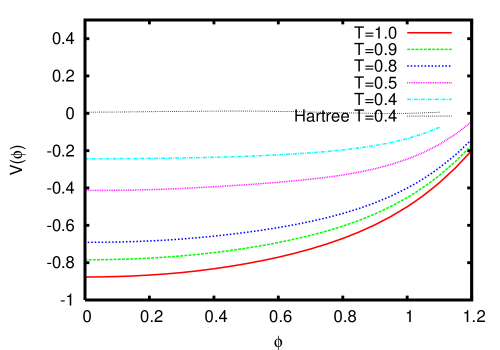
Figure 3: 2PI effective potential at NLO-$1/N$ for $N=4$ and $\lambda=0.5$.

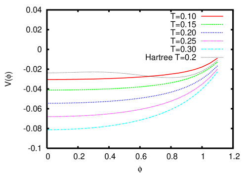
Figure 4: 2PI effective potential at NLO-$1/N$ for $N=4$ and $\lambda=0.1$.

In Fig. 5 we show the comparison between the Hartree, the 2PPI-NLO and Root’s NLO approximation (denoted as 1PI-NLO for short, cf. Appendix B) and the convergence towards the leading order large-$N$ results. These results are for $v=1$, $\lambda=0.5$ and $T=0.5$. As one sees, the effective potential in the 2PPI approximation is always in between those of the Hartree and 2PI-NLO approximation. The 1PI-NLO effective potential is close to the 2PI results. The latter two approximations differ only by terms of next-to-next-to-leading order (NNLO); it is surprising, nevertheless, that these terms are small already at moderate values of $N$. They are important for the evolution out of equilibrium, as they include scattering of quantum fluctuations. As for finite $N$ one expects differences to the large-$N$ result, the deviations of the various approximations from this limit do not a priori establish any “ranking”; however, the spontaneous symmetry breaking displayed by the Hartree and 2PPI-NLO approximations is certainly unphysical.

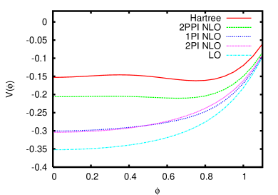
(a) $N=4$

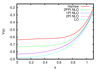
(b) $N=10$

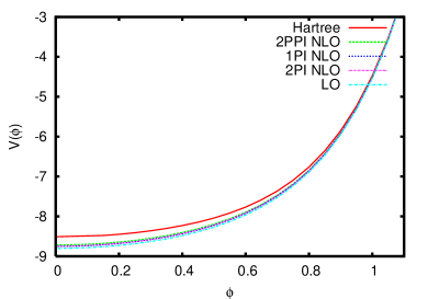
(c) $N=100$

Figure 5: Comparison of the effective potentials obtaind in the Hartree, 2PPI-NLO, 1PI-NLO, 2PI-NLO and leading order large-$N$ approximations for $\lambda=0.5$, $T=0.5$ and different values of $N$.

In Fig. 6 we display the spectral behavior of the effective momentum-dependent masses $m_{0}^{2}+\Sigma(\omega_{n},p)$, see Eqs.(2.28), at the equilibrium point $\phi=0$, for various temperatures, $N=4$ and $\lambda=0.5$. We plot these quantities versus the “Euclidean momentum” $p_{E}=\sqrt{\omega_{n}^{2}+p^{2}}$. The curves for various Matsubara frequencies $\omega_{n}$ are close together, implying an approximate rotation symmetry in the Euclidean $(\omega,p)$ plane. Whereas the large-momentum behavior is determined by an effective constant mass given by the tree level and bubble contributions, the effective masses at low momenta are considerably smaller, so that the various loop integrals are infrared-enhanced.

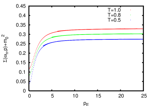
Figure 6: Momentum-dependent masses, cf. Eqs. (2.28), for different temperatures. $N=4$, $\lambda=0.5$. Here $p_{E}=\sqrt{\omega_{n}^{2}+p^{2}}$.

The infrared enhancement can also be seen in Fig. 7 where we plot, for $\lambda=0.1$, the values of the effective masses at the equilibrium point $\phi=0$. We display $m_{0}^{2}+\Sigma(0,0)$ and $m_{0}^{2}+\Sigma(0,p_{\rm max})$, where $p_{\rm max}$ is our pragmatic momentum cutoff. The values near $p=0$ are much smaller than those at $p_{\rm max}$, which can be considered as the asymptotic ones, see Fig. 6.

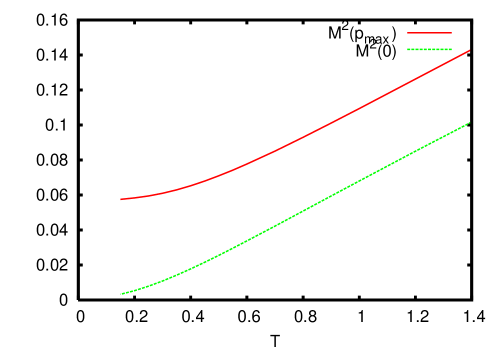
Figure 7: Temperature dependence of the effective masses $m_{0}^{2}+\Sigma(\omega,p)$ at $\omega=p=0$ and in the asymptotic region ($p=p_{\rm max}$) for $\lambda=0.1$ and $N=4$.

4 Conclusions

We have analyzed here the $O(N)$ linear sigma model in the 2PI formalism at next-to-leading order in a $1/N$ expansion. In order to do so, we have solved the coupled system of Euclidean Schwinger-Dyson equations for the $\sigma$ and $\pi$ propagators.

We have found that within our range of parameters the 2PI approximation does not display spontaneous symmetry breaking, as to be expected in a $1+1$ dimensional model. Furthermore, we find that the thermal propagators are enhanced in the infrared region. Due to momentum-dependent self-energy insertion the effective masses at low Euclidean momenta are smaller than those at large momenta.

We have compared the effective potential as a function of the external field $\phi$ to the ones obtained in several other approximations. The 1PI-NLO approximation is close to the 2PI-NLO one even for small $N$, whereas the potential obtained in the 2PPI-NLO approximation lies between those obtained in the Hartree and in the 2PI approximations. All potentials are above the large-$N$ effective potential and, of course, converge to it at large $N$. The Hartree and 2PPI-NLO approximations display spontaneous symmetry breaking, unphysical in $1+1$ dimensions. This is clearly an artefact of these approximations.

It would be of interest to extend the analysis of the $O(N)$ linear sigma model in the 2PI-NLO approximation to nonequilibrium systems. For the $O(N)$ model out of equilibrium the 2PPI approximation (to two loops in the effective action) displays a symmetric phase in the late time behavior [37], in contrast to what we have found here in thermal equilibrium.

Coming back to the simulations in $1+1$ dimensions for the case $N=1$ [28, 30] spontaneous symmetry breaking was found in the late time behavior of the Hartree approximation, whereas in both the 2PI and the 2PPI the mean field approaches the symmetric phase at late times. In contrast to that, the 2PPI approximation in equilibrium displays spontaneous symmetry breaking, and so does the 2PI approximation both with correct $N=1$ combinatorics and with $1/N$ combinatorics [38]. This is due to the fact that these calculations do not encompass kink transitions which are of order $1/\lambda$. So there remain some issues to be clarified.

In this work we were concerned mainly with the phase structure of the model in the 2PI scheme at next-to-leading order of the $1/N$ expansion. It would of course be useful to extend this analysis to $3+1$ dimensions using recently developed renormalizations techniques for 2PI-resummed perturbation theory [15, 16, 17, 18, 39]. Furthermore it would be interesting to compute various thermodynamic functions and transport coefficients [40, 41], in view of their relevance for heavy ion collisions.

Appendix A The 2PPI formalism to NLO of a $1/N$ expansion

In the 2PPI formalism [19, 20] one introduces a quadratic source term $K(x)\Phi^{2}(x)$ which, in contrast to the 2PI formalism, is local. The Legendre transformed variables are then $\phi(x)$ and $\Delta(x)$. For a comparison between the 2PI and 2PPI formalism see, e.g., Appendix A of Ref. [23]. For a translation invariant system $\phi$ and $\Delta$ are constants. The effective action then becomes an ordinary function of these variables. For the $O(N)$ system, the classical field is a vector $\vec{\Phi}_{\rm cl}=\hat{n}\phi$. As for the 2PI formalism we use a basis where the $\sigma$ field is in the direction $\hat{n}$ and the $N-1$ pion fields span the orthogonal directions. Then $\Delta$ is a $2\times 2$ matrix which becomes diagonal in this basis, with entries $\Delta_{\sigma}$ and $\Delta_{\pi}$. In contrast to the 2PI formalism, the Green functions take the simple form

$${\cal G}_{j}(p,\omega_{n})=\frac{1}{p^{2}+\omega_{n}^{2}+{\cal M}_{j}^{2}}$$ (A.1)

with the effective masses

$${\cal M}_{\sigma}^{2} = \lambda\left[3\phi^{2}-v^{2}+3\Delta_{\sigma}+(N-1)\Delta_{\pi}\right]$$ (A.2a)

$${\cal M}_{\pi}^{2} = \lambda\left[\phi^{2}-v^{2}+\Delta_{\sigma}+(N+1)\Delta_{\pi}\right]\;.$$ (A.2b)

Here the local mass insertions $\Delta_{j}$ are given by

$$\Delta_{j}=2\frac{\partial\Gamma^{\rm 2PPI}_{\rm q}}{\partial{\cal M}_{j}^{2}}\;.$$ (A.3)

where $\Gamma^{\rm 2PPI}_{\rm q}$ is the sum of all two particle point irreducible graphs. These are all graphs that do not fall apart if two internal lines meeting at one point are cut. They are computed with the propagators defined in Eq. (A.1). As for the 2PI formalism we have considered the derivatives with respect to ${\cal M}_{\pi}^{2}$ as the derivative with respect to the mass of one of the $(N-1)$ pion species, thus leaving out factors $(N-1)$ which anyway would cancel in the final formulae.

It is simpler to express the potential in terms of the effective masses ${\cal M}_{j}^{2}$ instead of the parameters $\Delta_{j}$. Then these gap equations can be derived from the effective potential

$$U_{\rm eff}(\phi,\mathcal{M}_{\sigma}^{2},\mathcal{M}^{2}_{\pi})=NU_{\rm cl}(\phi,\mathcal{M}_{\sigma}^{2},\mathcal{M}^{2}_{\pi})+U_{\rm q}(\phi,\mathcal{M}_{\sigma}^{2},\mathcal{M}^{2}_{\pi})\;.$$ (A.4)

Here $U_{\rm cl}$ is the“classical” potential [10, 23]

$$U_{\rm cl} = \frac{1}{2}{\cal M}_{\sigma}^{2}\phi^{2}-\frac{\lambda}{2}\phi^{4}-\frac{1}{2\lambda(N+2)}v^{2}\left\{{\cal M}_{\sigma}^{2}+(N-1){\cal M}_{\pi}^{2}\right\}$$

$$-\frac{1}{8\lambda(N+2)}\left[(N+1){\cal M}_{\sigma}^{4}+3(N-1){\cal M}_{\pi}^{4}-2(N-1){\cal M}_{\sigma}^{2}{\cal M}_{\pi}^{2}+2N\lambda^{2}v^{4}\right]\;,$$

which in this formulation already includes quantum parts through the effective masses. In this sense the separation between $U_{\rm cl}$ and the quantum part $U_{\rm q}$ is superficial. The basic contribution to $U_{\rm q}$ is the one-loop contribution

$$U_{\rm 1-loop}=U_{\rm 1-loop}^{\sigma}+(N-1)U_{\rm 1-loop}^{\pi}$$ (A.6)

with

$$U_{\rm 1-loop}^{j}=\frac{1}{2}{\rm Tr}\log\frac{{\cal G}_{j}}{{\cal G}_{j,0}}\;.$$ (A.7)

which explicitly reads

$$U^{j}_{\rm 1-loop}=\frac{1}{2}T\sum_{n}\int\frac{dp}{2\pi}\ln\frac{p^{2}+\omega_{n}^{2}+{\cal M}_{j}^{2}}{p^{2}+\omega_{n}^{2}+m_{j,0}^{2}}\;.$$ (A.8)

In regularized and renormalized form it becomes

$$U^{j}_{\rm 1-loop} = \frac{1}{2}T\sum_{n}\int\frac{dp}{2\pi}\left\{\ln\frac{p^{2}+\omega_{n}^{2}+{\cal M}_{j}^{2}}{p^{2}+\omega_{n}^{2}+m_{j,0}^{2}}\right.$$ (A.9)

$$\left.-\frac{{\cal M}_{j}^{2}-m_{j,0}^{2}}{p^{2}+\omega_{n}^{2}+m_{j,0}^{2}}\right\}+\frac{1}{2}({\cal M}_{j}^{2}-m_{j,0}^{2}){\cal B}_{j}\;.$$

The regularized bubble integrals have been defined in Eq. (2.11). If we include just $U_{\rm 1-loop}$ we again obtain the Hartree approximation with $\Delta_{j}={\cal B}_{j}$. The double-bubble diagrams are included here in the $U_{\rm cl}$ via the effective masses.

Going beyond the Hartree approximation in the 2PPI formalism in a strict $1/N$ expansion we only have to take into account “necklaces” and “generalized sunsets” and a 2PPI (but 2PR) combination of them. The necklace ${\cal N}$ takes the same form as for the 2PI formalism, see Eq. (2.22) and Fig.1, where of course the fish diagram, Eq. (2.21), is computed with the propagators of Eq. (A.1). The generalized sunset contribution is replaced by a more complex set of graphs. As discussed by Root [6], at next-to-leading order of $1/N$ the graphs with external lines have the form presented in Fig. 8, with alternating sigma propagators and necklaces. As the resemblance to a sunset becomes now very remote we refer to them as chain diagrams. These are summed up in the form

$${\cal C}=\frac{1}{2}T\sum_{m=-\infty}^{\infty}\int\frac{dq}{2\pi}\ln\left[1+{\bf S}(\omega_{m},q)\right]$$ (A.10)

where ${\bf S}(\omega_{m},q)$ is the kernel of the sunset diagram, Eq. (2.24):

$${\bf S}(\omega_{m},q)=-2\lambda\phi^{2}\frac{\lambda{\cal F}(\omega_{m},q)}{1+\lambda{\cal F}(\omega_{m},q)}{\cal G}_{\sigma}(\omega_{m},q)$$ (A.11)

In the 2PI formalism the higher powers of insertions ${\bf S}$ are included automatically, here the summation has to be done explicitly.

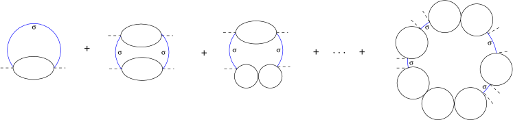
Figure 8: 2PPI or 1PI ”chain” contributions to the effective action.

If the graphs defined in the previous paragraph are introduced the quantum part of the effective potential takes the form

$$U_{\rm q}=U_{\rm 1-loop}+{\cal N}+{\cal C}$$ (A.12)

and the insertions $\Delta_{j}$ in the gap equations are given by

$$\Delta_{j}={\cal B}_{j}+2\frac{\partial{\cal N}}{\partial{\cal M}^{2}_{j}}+2\frac{\partial{\cal C}}{\partial{\cal M}^{2}_{j}}\;.$$ (A.13)

Explicitly the new contributions are given by

$$\frac{\partial{\cal N}}{\partial{\cal M}^{2}_{j}}=\frac{1}{2}\frac{\lambda}{N}T\sum_{n}\int\frac{dp}{2\pi}\frac{-\lambda{\cal F}(q,\omega_{n})}{1+\lambda{\cal F}(q,\omega_{n})}\frac{\partial{\cal F}_{j}}{\partial{\cal M}_{j}^{2}}(q,\omega_{n})$$ (A.14)

and

$$\frac{\partial{\cal C}}{\partial{\cal M}^{2}_{j}} = -\lambda\phi^{2}T\sum_{n}\int\frac{dq}{2\pi}\frac{1}{1+{\bf S}(\omega_{m},q)}\left\{\frac{\lambda}{N}\frac{1}{[1+\lambda{\cal F}(\omega_{m},q)]^{2}}\frac{\partial{\cal F}_{j}(\omega_{m},q)}{\partial{\cal M}_{j}^{2}}{\cal G}_{\sigma}(\omega_{n},q)\right.$$ (A.15)

$$\left.-\delta_{j\sigma}\frac{\lambda{\cal F}(\omega_{m},q)}{1+\lambda{\cal F}(\omega_{m},q)}{\cal G}_{\sigma}^{2}(\omega_{m},q)\right\}$$

Finally ${\cal F}=({\cal F}_{\sigma}+(N-1){\cal F}_{\pi})/N$ as before, and

$$\frac{\partial{\cal F}_{j}}{\partial{\cal M}_{j}^{2}}(p,\omega_{n})=-2T\sum_{M}\int\frac{dq}{2\pi}\frac{1}{(q^{2}+\omega_{m}^{2}+{\cal M}_{j}^{2})\,\left[(p-q)^{2}+(\omega_{n}-\omega_{m})^{2}+{\cal M}_{j}^{2}\right]^{2}}\;.$$ (A.16)

The partial derivative of $V_{\rm eff}$ with respect to $\phi$, divided by $N\phi$, in analogy to Eq. (2.29) is given by

$${\cal R}(\phi)={\cal M}_{\sigma}^{2}-2\lambda\phi^{2}+\frac{1}{N\phi}\frac{\delta{\cal C}}{\delta\phi}$$ (A.17)

with

$$\frac{1}{N\phi}\frac{\partial{\cal C}}{\partial\phi}=-2\frac{\lambda}{N}T\sum_{n}\int\frac{dq}{2\pi}\frac{1}{1+{\bf S}(\omega_{m},q)}\frac{{\cal F}(\omega_{m},q)}{1+\lambda{\cal F}(\omega_{m},q)}{\cal G}_{\sigma}(\omega_{m},q)$$ (A.18)

Appendix B The 2PPI formalism to NLO of a $1/N$ expansion

In a seminal article [6] Root has discusssed the extension to the next-to-leading order in a $1/N$ expansion within the 1PI formalism. He introduces an auxiliary field $\chi$ which in the language used throughout our work can be identified with a self-consistent pion mass ${\cal M}_{\pi}^{2}$. The classical potential then takes the form

$$U_{\rm cl}(\phi,{\cal M}_{\pi}^{2})=N\left(\frac{1}{2}{\cal M}_{\pi}^{2}(\phi^{2}-v^{2})-\frac{{\cal M}_{\pi}^{4}}{4\lambda}\right)\;,$$ (B.1)

it can be obtained by taking the large-$N$ limit of the analogous potential of the 2PPI formalism, Eq. (A), when the mass of the $\sigma$ propagator is given by

$${\cal M}_{\sigma}^{2}={\cal M}_{\pi}^{2}+2\lambda\phi^{2}\;.$$ (B.2)

To leading order in $1/N$ this would follow in the 2PPI formalism when taking only the pions into account in the one-loop terms. In Root’s work this relation is kept fixed for all orders of $1/N$, however. In a strict $1/N$ counting one may indeed neglect corrections of NLO to the propagator, as actually suggested in Root’s work by using the leading order gap equation. As in the 2PPI formalism the propagators take the tree level form of Eq. (A.1).

In the following we will rewrite the various terms included by Root in a way that makes the correspondence to the other formalisms more transparent. Including the next-to-leading order corrections the one-loop term takes the form of Eqs. (A.7)-(A.9), with ${\cal M}_{\sigma}^{2}$ given by Eq. (B.2). As in the 2PPI formalism the next terms are the necklace and the chain diagrams. In the necklace part only the pion fish diagram is taken into account. The definition of the necklace contribution is then identical to the one in the 2PI formalism, Eq. (2.22) with the modification that ${\cal F}\equiv{\cal F}_{\pi}$ and that the propagators in the fish graph, Eq. (2.21) are given by Eq. (A.1).

The chain diagram ${\cal C}$ takes the same form as in the 2PPI formalism, see Eqs. (A.10) and (A.11), of course now with ${\cal F}={\cal F}_{\pi}$. In taking the derivatives the sigma propagator is now considered as a function of ${\cal M}_{\pi}^{2}$ and $\phi$. The modifications with respect to the 2PPI formalism are obvious. We have

$$\frac{\partial{\cal C}}{\partial{\cal M}^{2}_{\pi}} = -\lambda\phi^{2}T\sum_{n}\int\frac{dq}{2\pi}\frac{1}{1+{\bf S}(\omega_{m},q)}\left\{\frac{\lambda}{N}\frac{1}{[1+\lambda{\cal F}(\omega_{m},q)]^{2}}\frac{\partial{\cal F}_{j}(\omega_{m},q)}{\partial{\cal M}_{\pi}^{2}}{\cal G}_{\sigma}(\omega_{n},q)\right.$$ (B.3)

$$\left.-\frac{\lambda{\cal F}(\omega_{m},q)}{1+\lambda{\cal F}(\omega_{m},q)}{\cal G}_{\sigma}^{2}(\omega_{m},q)\right\}$$

and

$$\frac{1}{N\phi}\frac{\partial{\cal C}}{\partial\phi}=-2\frac{\lambda}{N}T\sum_{n}\int\frac{dq}{2\pi}\frac{1}{1+{\bf S}(\omega_{m},q)}\frac{{\cal F}(\omega_{m},q)}{1+\lambda{\cal F}(\omega_{m},q)}{\cal G}_{\sigma}(\omega_{m},q)\left[1-2\lambda\phi^{2}{\cal G}_{\sigma}(\omega_{m},q)\right]\;.$$ (B.4)

Finally the gap equation is

$${\cal M}_{\pi}^{2}=\lambda\left(\phi^{2}-v^{2}+2\frac{\partial{\cal N}}{\partial{\cal M}^{2}_{\pi}}+2\frac{\partial{\cal C}}{\partial{\cal M}^{2}_{\pi}}\right)$$ (B.5)

where $\partial{\cal N}/\partial{\cal M}^{2}_{\pi}$ is given by Eq. (A.14), and the quantity ${\cal R}$ is given by

$${\cal R}(\phi)={\cal M}_{\sigma}^{2}-2\lambda\phi^{2}+\frac{1}{N\phi}\frac{\delta{\cal C}}{\delta\phi}\;.$$ (B.6)

References

- [1] D. A. Kirzhnits and A. D. Linde, Sov. Phys. JETP. 40, 628 (1975).
- [2] S. R. Coleman, R. Jackiw and H. D. Politzer, Phys. Rev. D10, 2491 (1974).
- [3] L. Dolan and R. Jackiw, Phys. Rev. D9, 3320 (1974).
- [4] W. A. Bardeen and M. Moshe, Phys. Rev. D28, 1372 (1983).
- [5] H. J. Schnitzer, Phys. Rev. D10, 1800 (1974).
- [6] R. G. Root, Phys. Rev. D10, 3322 (1974).
- [7] S. R. Coleman, Commun. Math. Phys. 31, 259 (1973).
- [8] G. Amelino-Camelia and S.-Y. Pi, Phys. Rev. D47, 2356 (1993), [hep-ph/9211211].
- [9] G. Amelino-Camelia, Phys. Lett. B407, 268 (1997), [hep-ph/9702403].
- [10] Y. Nemoto, K. Naito and M. Oka, Eur. Phys. J. A9, 245 (2000), [hep-ph/9911431].
- [11] J. T. Lenaghan and D. H. Rischke, J. Phys. G26, 431 (2000), [nucl-th/9901049].
- [12] H. Verschelde and J. De Pessemier, Eur. Phys. J. C22, 771 (2002), [hep-th/0009241].
- [13] J. Baacke and S. Michalski, Phys. Rev. D65, 065019 (2002), [hep-ph/0109137].
- [14] J. M. Cornwall, R. Jackiw and E. Tomboulis, Phys. Rev. D10, 2428 (1974).
- [15] H. van Hees and J. Knoll, Phys. Rev. D65, 025010 (2002), [hep-ph/0107200].
- [16] H. Van Hees and J. Knoll, Phys. Rev. D65, 105005 (2002), [hep-ph/0111193].
- [17] H. van Hees and J. Knoll, Phys. Rev. D66, 025028 (2002), [hep-ph/0203008].
- [18] J.-P. Blaizot, E. Iancu and U. Reinosa, Nucl. Phys. A736, 149 (2004), [hep-ph/0312085].
- [19] H. Verschelde and M. Coppens, Phys. Lett. B287, 133 (1992).
- [20] M. Coppens and H. Verschelde, Z. Phys. C58, 319 (1993).
- [21] H. Verschelde, Phys. Lett. B497, 165 (2001), [hep-th/0009123].
- [22] G. Smet, T. Vanzielighem, K. Van Acoleyen and H. Verschelde, Phys. Rev. D65, 045015 (2002), [hep-th/0108163].
- [23] J. Baacke and S. Michalski, Phys. Rev. D67, 085006 (2003), [hep-ph/0210060].
- [24] J. Berges, Nucl. Phys. A699, 847 (2002), [hep-ph/0105311].
- [25] G. Aarts, D. Ahrensmeier, R. Baier, J. Berges and J. Serreau, Phys. Rev. D66, 045008 (2002), [hep-ph/0201308].
- [26] J. Berges and J. Cox, Phys. Lett. B517, 369 (2001), [hep-ph/0006160].
- [27] G. Aarts and J. Berges, Phys. Rev. Lett. 88, 041603 (2002), [hep-ph/0107129].
- [28] F. Cooper, J. F. Dawson and B. Mihaila, Phys. Rev. D67, 056003 (2003), [hep-ph/0209051].
- [29] J. Baacke and A. Heinen, Phys. Rev. D67, 105020 (2003), [hep-ph/0212312].
- [30] J. Baacke and A. Heinen, Phys. Rev. D68, 127702 (2003), [hep-ph/0305220].
- [31] D. Y. Grigoriev and V. A. Rubakov, Nucl. Phys. B299, 67 (1988).
- [32] M. G. Alford, H. Feldman and M. Gleiser, Phys. Rev. Lett. 68, 1645 (1992).
- [33] F. J. Alexander and S. Habib, Phys. Rev. Lett. 71, 955 (1993), [hep-th/9212059].
- [34] M. Salle, Phys. Rev. D69, 025005 (2004), [hep-ph/0307080].
- [35] S. R. Coleman, Phys. Rev. D11, 2088 (1975).
- [36] S.-J. Chang, Phys. Rev. D13, 2778 (1976).
- [37] A. Heinen, in preparation .
- [38] J. Baacke and S. Michalski, unpublished results .
- [39] F. Cooper, B. Mihaila and J. F. Dawson, hep-ph/0407119.
- [40] G. Aarts and J. M. Martinez Resco, Phys. Rev. D68, 085009 (2003), [hep-ph/0303216].
- [41] G. Aarts and J. M. Martinez Resco, JHEP 02, 061 (2004), [hep-ph/0402192].