Abstract

The energy-momentum relations for massive and massless particles are $E=p^{2}/2m$ and $E=pc$ respectively. According to Einstein, these two different expressions come from the same formula $E=\sqrt{(cp)^{2}+m^{2}c^{4}}$. Quarks and partons are believed to be the same particles, but they have quite different properties. Are they two different manifestations of the same covariant entity as in the case of Einstein’s energy-momentum relation? The answer to this question is YES. It is possible to construct harmonic oscillator wave functions which can be Lorentz-boosted. They describe quarks bound together inside hadrons. When they are boosted to an infinite-momentum frame, these wave functions exhibit all the peculiar properties of Feynman’s parton picture. This formalism leads to a parton distribution corresponding to the valence quarks, with a good agreement with the experimentally observed distribution.

1 Introduction

Since Einstein’s formulation of special relativity in 1905, the most significant addition to physics was quantum mechanics based on wave-particle duality. The question then is whether relativity is consistent with quantum mechanics. The answer to this question is very simple for plane waves, because they can can be written in a Lorentz-invariant form. Because of this mathematical simplicity, it is possible to construct quantum field theory with Feynman diagrams as a computational tool.

How about standing waves? Are they consistent with Einstein’s relativity? This question has not been properly addressed. The question is how standing waves in one Lorentz frame would look in a different Lorentz frame. While we are not able to address this problem in general terms, we would like to point out that there is at least one set of wave functions which can be Lorentz-boosted. It is the set of solutions of the Lorentz-invariant harmonic oscillator equation proposed by Feynman et al. in 1971 [1]. The solutions given in their papers are not normalizable in time-separation variable and do not correspond to physics.

However, there are more than two hundred solutions satisfying different boundary conditions. We choose the solutions which are localized and normalizable in both space and time coordinates. We shall call this set of solutions covariant harmonic oscillators. These solutions have the following common properties:

• The formalism is consistent with established physical principles including the uncertainty principle in quantum mechanics and the transformation laws of special relativity [2].

• The formalism is consistent with the basic hadronic features observed in high-energy laboratories, including hadronic mass spectra, the proton form factor, and the parton phenomena [2].

• The formalism constitutes a representation of Wigner’s little of the Poincaré group which dictates internal space-time symmetries of relativistic particles [2, 3]. The little group is the maximal subgroup of the Lorentz group which leaves the four-momentum of a given particle invariant.

In this paper, we use this covariant oscillator formalism to see that the quark model and the parton models are two different manifestations of one covariant formalism. We shall see how the parton picture emerges from the Lorentz-boosted hadronic wave function. In Sec. 2, we introduce the basic ingredients of the covariant harmonic oscillator formalism. In Sec. 4, we use this formalism to show that the valance quark distribution in the proton structure function can be derived from the Lorentz-boosted quark-model wave function.

2 Covariant Harmonic Oscillators

The covariant harmonic oscillator formalism has been discussed exhaustively in the literature, and it is not necessary to give another full-fledged treatment in the present paper. We shall discuss here only its features needed for explaining the peculiarities of Feynman’s parton picture.

Let us consider a bound state of two particles. Then there is a Bohr-like radius measuring the space-like separation between the quarks. There is also a time-like separation between the quarks, and this variable becomes mixed with the longitudinal spatial separation as the hadron moves with a relativistic speed. There are no quantum excitations along the time-like direction. On the other hand, there is the time-energy uncertainty relation which allows quantum transitions. The covariant oscillator formalism can accommodate these aspects within the framework of the present form of quantum mechanics. The uncertainty relation between the time and energy variables is the c-number relation [4], which does not allow excitations along the time-like coordinate. This aspect is illustrated in Fig. 1.

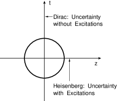
Figure 1: Quantum mechanics with the c-number time-energy uncertainty relation. The present form of quantum mechanics allows quantum excitations along the space-like directions, but does not allow excitations along the time-like direction even though there is an uncertainty relation between the time and energy variables.

Let us consider now a hadron consisting of two quarks. If the space-time position of two quarks are specified by $x_{a}$ and $x_{b}$ respectively, the system can be described by the variables

$$X=(x_{a}+x_{b})/2,\qquad x=(x_{a}-x_{b})/2\sqrt{2}.$$ (1)

The four-vector $X$ specifies where the hadron is located in space and time, while the variable $x$ measures the space-time separation between the quarks. In the convention of Feynman et al. [1], the internal motion of the quarks bound by a harmonic oscillator potential of unit strength can be described by the Lorentz-invariant equation

$$\frac{1}{2}\left\{x^{2}_{\mu}-\frac{\partial^{2}}{\partial x_{\mu}^{2}}\right\}\psi(x)=\lambda\psi(x).$$ (2)

We use here the metric: $x^{\mu}=(x,y,z,t)$.

If the hadron is at rest, we can consider a solution of the form

$$\psi(x,y,z,t)=\psi(x,y,z)\left(\frac{1}{\pi}\right)^{1/4}\exp{\left(-t^{2}/2\right)},$$ (3)

where $\psi(x,y,z)$ is the wave function for the three-dimensional oscillator with appropriate angular momentum quantum numbers. Indeed, the above wave function constitutes a representation of Wigner’s $O(3)$-like little group for a massive particle [2]. In the above expression, there are no time-like excitations, and this is consistent with what we see in the real world.

Since the three-dimensional oscillator differential equation is separable in both spherical and Cartesian coordinate systems, $\psi(x,y,z)$ consists of Hermite polynomials of $x,y$, and $z$. If the Lorentz boost is made along the $z$ direction, the $x$ and $y$ coordinates are not affected, and can be dropped from the wave function. The wave function of interest can be written as

$$\psi^{n}(z,t)=\left(\frac{1}{\pi}\right)^{1/4}\exp{\left(-t^{2}/2\right)}\psi_{n}(z),$$ (4)

with

$$\psi^{n}(z)=\left(\frac{1}{\pi n!2^{n}}\right)^{1/2}H_{n}(z)\exp(-z^{2}/2),$$ (5)

where $\psi^{n}(z)$ is for the $n$-th excited oscillator state. The full wave function $\psi^{n}(z,t)$ is

$$\psi^{n}_{0}(z,t)=\left(\frac{1}{\pi n!2^{n}}\right)^{1/2}H_{n}(z)\exp\left\{-\frac{1}{2}\left(z^{2}+t^{2}\right)\right\}.$$ (6)

The subscript $0$ means that the wave function is for the hadron at rest. The above expression is not Lorentz-invariant, and its localization a deformation as the hadron moves along the $z$ direction [2]. This is still a Lorentz-covariant expression, and this form satisfies the Lorentz-invariant differential equation of Eq.(2) even if the $z$ and $t$ variables are given by

$$(\cosh\eta)z-(\sinh\eta)t,\qquad(\cosh\eta)t-(\sinh\eta)z.\qquad$$ (7)

This corresponds to a Lorentz-boosting of the system along the $z$ direction with the boost parameter $\eta.$ This becomes more transparent if we use the light-cone if we use the light-cone coordinate system where

$$u=(z+t)/\sqrt{2},\qquad v=(z-t)/\sqrt{2},$$ (8)

as is illustrated in Fig. 2. Here one coordinate is becoming expanded while the other become contracted. This type of deformation is called “squeeze” these days [5],

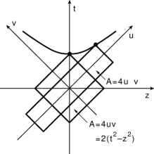
Figure 2: Space-time picture of the Lorentz boost. The invariant quantity $(z^{2}-t^{2})$ can be written as $(z+t)(z-t)$. This is proportional to the product of the light-cone variables $u=(z+t)/\sqrt{2}$ and $(z-t)/\sqrt{2}$.

The wave function becomes

$$\psi_{0}(z,t)=\left(\frac{1}{\pi}\right)^{1/2}\exp\left\{-\frac{1}{2}(u^{2}+v^{2})\right\},$$ (9)

where we have left out the Hermite polynomials for simplicity, because the essential properties of the oscillator wave functions are dominated by their Gaussian factor.

If the system is boosted variables $u$ and $v$ are replaced by $e^{-\eta}u$ and $e^{eta}v$ respectively, as is illustrated in Fig. 2. and the Lorentz-squeezed wave function becomes

$$\psi_{\eta}(z,t)=\left(\frac{1}{\pi}\right)^{1/2}\exp\left\{-\frac{1}{2}\left(e^{-2\eta}u^{2}+e^{2\eta}v^{2}\right)\right\}.$$ (10)

The transition from Eq.(9) to Eq.(10) is illustrated in Fig. 3. We can produce this figure by combining quantum mechanics of Fig. 1 and special relativity of Fig. 2.

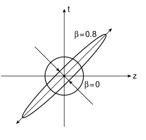
Figure 3: Effect of the Lorentz boost on the space-time wave function. The circular space-time distribution at the rest frame becomes Lorentz-squeezed to become an elliptic distribution.

3 Feynman’s Parton Picture

In 1969 [6], Feynman observed the following peculiarities in his parton picture of hadrons.

• The picture is valid only for hadrons moving with velocity close to that of light.

• The interaction time between the quarks becomes dilated, and partons behave as free independent particles.

• The momentum distribution of partons becomes widespread as the hadron moves fast.

• The number of partons seems to be infinite or much larger than that of quarks.

Because the hadron is believed to be a bound state of two or three quarks, each of the above phenomena appears as a paradox, particularly 2) and 3) together. We would like to resolve this paradox using the covariant harmonic oscillator formalism.

For this purpose, we need a momentum-energy wave function. If the quarks have the four-momenta $p_{a}$ and $p_{b}$, we can construct two independent four-momentum variables [1]:

$$P=p_{a}+p_{b},\qquad q=\sqrt{2}(p_{a}-p_{b}).$$ (11)

The four-momentum $P$ is the total four-momentum and is thus the hadronic four-momentum. $q$ measures the four-momentum separation between the quarks.

We expect to get the momentum-energy wave function by taking the Fourier transformation of Eq.(10):

$$\phi_{\eta}(q_{z},q_{0})=\left(\frac{1}{2\pi}\right)\int\psi_{\eta}(z,t)\exp{\left\{-i(q_{z}z-q_{0}t)\right\}}dxdt.$$ (12)

Let us now define the momentum-energy variables in the light-cone coordinate system as

$$q_{u}=(q_{0}-q_{z})/\sqrt{2},\qquad q_{v}=(q_{0}+q_{z})/\sqrt{2}.$$ (13)

In terms of these variables, the Fourier transformation of Eq.(12) can be written as

$$\phi_{\eta}(q_{z},q_{0})=\left(\frac{1}{2\pi}\right)\int\psi_{\eta}(z,t)\exp{\left\{-i(q_{u}u+q_{v}v)\right\}}dudv.$$ (14)

The resulting momentum-energy wave function is

$$\phi_{\eta}(q_{z},q_{0})=\left(\frac{1}{\pi}\right)^{1/2}\exp\left\{-\frac{1}{2}\left(e^{-2\eta}q_{u}^{2}+e^{2\eta}q_{v}^{2}\right)\right\}.$$ (15)

Because we are using here the harmonic oscillator, the mathematical form of the above momentum-energy wave function is identical to that of the space-time wave function. The Lorentz squeeze properties of these wave functions are also the same, as is indicated in Fig. 4.

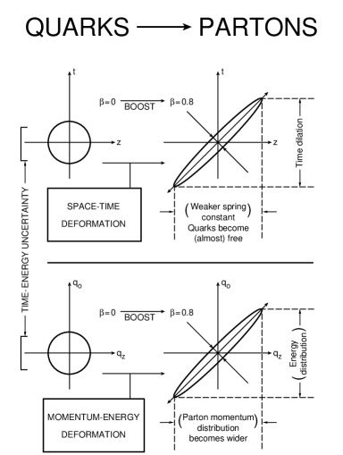
Figure 4: Lorentz-squeezed space-time and momentum-energy wave functions. As the hadron’s speed approaches that of light, both wave function become concentrated along their respective positive light-cone axes. These light-cone concentrations lead to Feynman’s parton picture.

When the hadron is at rest with $\eta=0$, both wave functions behave like those for the static bound state of quarks. As $\eta$ increases, the wave functions become continuously squeezed until they become concentrated along their respective positive light-cone axes. Let us look at the z-axis projection of the space-time wave function. Indeed, the width of the quark distribution increases as the hadronic speed approaches that of the speed of light. The position of each quark appears widespread to the observer in the laboratory frame, and the quarks appear like free particles.

Furthermore, interaction time of the quarks among themselves become dilated. Because the wave function becomes wide-spread, the distance between one end of the harmonic oscillator well and the other end increases as is indicated in Fig. 3. This effect, first noted by Feynman [6], is universally observed in high-energy hadronic experiments. Let us look at the time ratio more carefully. The period of oscillation increases like $e^{\eta}$ as was predicted by Feynman [6].

In the picture of the Lorentz squeezed hadron given in Fig. 3, the hadron moves along the $u$ (positive light-cone) axis, while the external signal moves in the direction opposite to the hadronic momentum, which corresponds to the $v$ (negative light-cone) axis. This time interval is proportional to the minor axis of the ellipse given in Fig. 3.

If we use $T_{ext}$ and $T_{osc}$ for the quark’s interaction time with the external signal and the interaction time among the quarks, their ratio becomes

$$\frac{T_{ext}}{T_{osc}}=\frac{\exp(-\eta)}{\exp(\eta)}=\exp(-2\eta).$$ (16)

The ratio of the interaction time to the oscillator period becomes $e^{-2\eta}$. The energy of each proton coming out of the Fermilab accelerator is $900GeV$. This leads to the ratio to $10^{-6}$. This is indeed a small number. The external signal is not able to sense the interaction of the quarks among themselves inside the hadron. Thus, the quarks appear to be free particles to the external signal. This is the cause of incoherence in the parton interaction amplitudes. The momentum-energy wave function is just like the space-time wave function in the oscillator formalism. The longitudinal momentum distribution becomes wide-spread as the hadronic speed approaches the velocity of light. This is in contradiction with our expectation from nonrelativistic quantum mechanics that the width of the momentum distribution is inversely proportional to that of the position wave function. Our expectation is that if the quarks are free, they must have their sharply defined momenta, not a wide-spread distribution. This apparent contradiction presents to us the following two fundamental questions:

• If both the spatial and momentum distributions become widespread as the hadron moves, and if we insist on Heisenberg’s uncertainty relation, is Planck’s constant dependent on the hadronic velocity?

• Is this apparent contradiction related to another apparent contradiction that the number of partons is infinite while there are only two or three quarks inside the hadron?

The answer to the first question is “No”, and that for the second question is “Yes”. Let us answer the first question which is related to the Lorentz invariance of Planck’s constant. If we take the product of the width of the longitudinal momentum distribution and that of the spatial distribution, we end up with the relation

$$<z^{2}><q_{z}^{2}>=(1/4)[\cosh(2\eta)]^{2}.$$ (17)

The right-hand side increases as the velocity parameter increases. This could lead us to an erroneous conclusion that Planck’s constant becomes dependent on velocity. This is not correct, because the longitudinal momentum variable $q_{z}$ is no longer conjugate to the longitudinal position variable when the hadron moves.

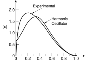
Figure 5: Calculation of the parton distribution from a hadronic wave function in the static quark model. The covariant harmonic oscillator formalism produces the quark-model wave function for hadrons at rest. The same formalism produces the parton distribution function in the infinite-momentum frame. The valence parton distribution calculated in this way is compared with the distribution observed in high-energy laboratories. This graph shows a good agreement between the oscillator-based theory and the observed experimental data.

In order to maintain the Lorentz-invariance of the uncertainty product, we have to work with a conjugate pair of variables whose product does not depend on the velocity parameter. Let us go back to Eq.(13) and Eq.(14). It is quite clear that the light-cone variable $u$ and $v$ are conjugate to $q_{u}$ and $q_{v}$ respectively. It is also clear that the distribution along the $q_{u}$ axis shrinks as the $u$-axis distribution expands. The exact calculation leads to

$$<u^{2}><q_{u}^{2}>=1/4,\qquad<v^{2}><q_{v}^{2}>=1/4.$$ (18)

Planck’s constant is indeed Lorentz-invariant.

Let us next resolve the puzzle of why the number of partons appears to be infinite while there are only a finite number of quarks inside the hadron. As the hadronic speed approaches the speed of light, both the $x$ and $q$ distributions become concentrated along the positive light-cone axis. This means that the quarks also move with velocity very close to that of light. Quarks in this case behave like massless particles.

We then know from statistical mechanics that the number of massless particles is not a conserved quantity. For instance, in black-body radiation, free light-like particles have a widespread momentum distribution. However, this does not contradict the known principles of quantum mechanics, because the massless photons can be divided into infinitely many massless particles with a continuous momentum distribution.

Likewise, in the parton picture, massless free quarks have a wide-spread momentum distribution. They can appear as a distribution of an infinite number of free particles. These free massless particles are the partons. It is possible to measure this distribution in high-energy laboratories, and it is also possible to calculate it using the covariant harmonic oscillator formalism. We are thus forced to compare these two results [7]. Figure 5 shows the result.

Concluding Remarks

In this report, we introduced first the covariant harmonic oscillator formalism which is consistent with all physical laws of quantum mechanics and special relativity. We then used this this formalism to show that the quark model and the parton model are two limiting case of one covariant picture of quantum bound states.

References

- [1] R. P. Feynman, M. Kislinger, and F. Ravndal, Phys. Rev. D 3, 2706 (1971).
- [2] Y. S. Kim and M. E. Noz, Theory and Applications of the Poincaré Group (Reidel, Dordrecht, 1986).
- [3] E. P. Wigner, Ann. Math. 40, 149 (1939).
- [4] P. A. M. Dirac, Proc. Roy. Soc. (London) A114, 243 and 710 (1927).
- [5] Y. S. Kim and M. E. Noz, Phase Space Picture of Quantum Mechanics (World Scientific, 1991).
- [6] R. P. Feynman, in High Energy Collisions, Proceedings of the Third International Conference, Stony Brook, New York, C. N. Yang et al., eds. (Gordon and Breach, New York, 1969).
- [7] P. E. Hussar, Phys. Rev. D 23, 2781 (1981).