A precise analytical description of the Earth matter effect on oscillations of low energy neutrinos

Abstract

We present a formalism for the matter effects in the Earth on low energy neutrino fluxes which is both accurate and has all advantages of a full analytic treatment. The oscillation probabilities are calculated up to second order term in $\epsilon(x)\equiv 2V(x)E/\Delta m^{2}$ where $V(x)$ is the neutrino potential at position $x$. We show the absence of large undamped phases which makes the expansion in $\epsilon$ well behaved. An improved expansion is presented in terms of the variation of $V(x)$ around a suitable mean value which allows to treat energies up to those relevant for Supernova neutrinos. We discuss also the case of three-neutrino mixing.

I Introduction

The propagation of low energy neutrinos in the Earth w ; MS86 ; DN is an important aspect of physics of solar w - sk-dn and Supernova (SN) neutrinos DS - DKRT . It will be useful in determining the oscillation parameters, and, in future, to search for effects of 1-3 mixing ohl and for a ’tomography’ of the Earth (see, e.g. IS ; LOTW ). It might even be possible to look for small structures of the density profile IS .

In the existing calculations of Earth matter effects (see, e.g.  w - IS ) the density profile is often approximated by one, two or several layers (mainly mantle and core) with constant densities or a direct numerical integration of the evolution equation is performed. However, the emergence of the large mixing MSW solution to the solar neutrino problem opens a more efficient approach to the oscillation effects in the Earth. Indeed, for the LMA parameters, the oscillations of the solar and (lower energy) supernova neutrinos inside the Earth occur in a ’weak’ regime, where the matter potential $V$ is much smaller than the ’kinetic energy’ of the neutrino system, i.e.

$$V(x)\ll\frac{\Delta m^{2}}{2E}.$$ (1)

Here $V(x)\equiv\sqrt{2}G_{F}N_{e}(x)$, $G_{F}$ is the Fermi constant, $N_{e}(x)$ is the number density of the electrons, $\Delta m^{2}\equiv m^{2}_{2}-m^{2}_{1}$ is the mass squared difference, and $E$ is the neutrino energy.

In this case one can introduce a small parameter

$$\epsilon(x) \equiv {2EV(x)\over\Delta m^{2}}$$

$$= 0.02\cdot\left[{E\over 10\,{\rm MeV}}\right]\cdot\left[{N_{e}(x)\over N_{A}}\right]\cdot\left[{7.7\cdot 10^{-5}\,{\rm eV}^{2}\over\Delta m^{2}}\right],$$

where $N_{A}$ is the Avogadro number, and consider an expansion of the oscillation probabilities in $\epsilon(x)$.

In ref. Ioannisian:2004jk , the $\epsilon$ perturbation theory was formulated in the basis of neutrino mass states $\nu_{mass}\equiv(\nu_{1},\nu_{2})^{T}$. The oscillation probabilities and the regeneration factor were calculated to first order in $\epsilon$. The expressions obtained are valid for arbitrary density profiles with sufficiently low density (1). They simplify the numerical calculations substantially and allow to understand in details all features of the oscillation effects. The method reproduced immediately the analytic result obtained in HLS for an approximate but realistic density profile. Similar integral expression for the regeneration factor has been discussed in Akhmedov:2004rq .

Since $\epsilon(x)$ increases with energy, the lowest approximation in $\epsilon(x)$ may not be enough for larger energies. For instance, if $E\simeq 50$ MeV (possible for SN neutrinos), we find $\epsilon(x)\simeq 0.6$ at the center of the Earth.

The purpose of this paper is to improve on this method and obtain accurate formulas which are valid for higher energies. In section 2 the oscillation probabilities are calculated in second order in $\epsilon(x)$ and the convergence of the $\epsilon$ expansion is commented on. In section 3 we suggest an improved perturbation theory which allows one to extend the expansion to higher energies. The generalization to three neutrinos is given in section 4 and a brief conclusion in section 5.

II Second order corrections to the oscillation probabilities

In this and the following section we consider the mixing of two (active) neutrinos $\nu_{f}=U(\theta)\nu_{mass}$, where $\nu_{f}\equiv(\nu_{e},\nu_{a})^{T}$ and $\nu_{mass}\equiv(\nu_{1},\nu_{2})^{T}$ are the flavor and mass states, respectively and $\nu_{a}$ is a linear combination of $\nu_{\mu}$ and $\nu_{\tau}$. $U(\theta)$ and $\theta$ are the mixing matrix and mixing angle in vacuum. We define the matrix $U(\alpha)$ as

$$U(\alpha)\equiv\left(\begin{tabular}[]{rr}$\cos\alpha$&$\sin\alpha$\\ $-\sin\alpha$&$\cos\alpha$\end{tabular}\right).$$ (3)

In  Ioannisian:2004jk the following expression for the $S$-matrix in the mass eigenstates basis was derived :

$$S = \left(\!\begin{tabular}[]{cc}1&0\\ 0&$e^{\!\!\!-i\phi^{m}_{x_{0}\to x_{f}}}$\end{tabular}\!\!\!\!\right)+$$ (19)

$$-i\int_{x_{0}}^{x_{f}}dx\left(\!\begin{tabular}[]{cc}1&0\\ 0&$e^{\!\!\!-i\phi^{m}_{x\to x_{f}}}$\end{tabular}\!\!\!\!\right)\Upsilon(x)\left(\!\begin{tabular}[]{cc}1&0\\ 0&$e^{\!\!\!-i\phi^{m}_{x_{0}\to x}}$\end{tabular}\!\!\!\!\right)-$$

$$-\!\int_{x_{0}}^{x_{f}}\!\!\!\!\!dx\int_{x_{0}}^{x}\!\!\!\!\!dy\left(\!\begin{tabular}[]{cc}1&0\\ 0&$e^{\!\!\!-i\phi^{m}_{x\to x_{f}}}$\end{tabular}\!\!\!\!\right)\Upsilon(x)\left(\!\begin{tabular}[]{cc}1&0\\ 0&$e^{\!\!\!-i\phi^{m}_{y\to x}}$\end{tabular}\!\!\!\!\right)\Upsilon(y)\left(\!\begin{tabular}[]{cc}1&0\\ 0&$e^{\!\!\!-i\phi^{m}_{x_{0}\to y}}$\end{tabular}\!\!\!\!\right)$$

$$+\cdots,$$

where

$$\phi^{m}_{x_{1}\to x_{2}}\equiv\int_{x_{1}}^{x_{2}}dx\Delta^{m}(x)$$ (20)

is the adiabatic phase difference acquired by the neutrino eigenstates in matter on their trajectory between two points $x_{1}$ and $x_{2}$. $\Delta^{m}(x)$ is defined as

$$\Delta^{m}(x)\equiv{\Delta m^{2}\over 2E}\sqrt{1-2\epsilon(x)\cos 2\theta+\epsilon(x)^{2}}\ ;$$ (21)

in vacuum we obviously have

$$\Delta^{m}\rightarrow\Delta\equiv{\Delta m^{2}\over 2E}.$$ (22)

The $S$-matrix in (19) is written as a perturbative expansion in $\Upsilon(x)$ where

$$\Upsilon(x)={\sin 2\theta\over 2}~{}V(x)\left(\begin{tabular}[]{cc}0&1\\ 1&0\end{tabular}\right)+{1\over 2}\Delta^{m}(x)\sin^{2}\theta^{\prime}\left(\begin{tabular}[]{cc}1&0\\ 0&-1\end{tabular}\right).$$ (23)

$\theta^{\prime}$ is the mixing angle of the mass eigenstates in matter,

$$\sin 2\theta^{\prime}\!={\epsilon\ \sin 2\theta\over\sqrt{(\cos 2\theta-\epsilon)^{2}\!\!+\!\sin^{2}2\theta}}=\epsilon\sin 2\theta^{m},$$ (24)

and $\theta^{m}=\theta+\theta^{\prime}$ is the corresponding mixing angle of the flavor states.

The $S$-matrix in eq.(19) refers to a straight path through the earth from the entry point $x_{0}$ to an exit point $x_{f}$ and the coordinate $x$ is measured along the path. For notational convenience, we do not put labels $x_{0},x_{f}$, etc. on $S$.

Using eq. (23), we obtain the $S$ matrix in terms of the potential $V$:

$$S\!\!\! = \!\!\left(\!\begin{tabular}[]{cc}1&0\\ 0&$e^{\!\!\!-i\phi^{m}_{x_{0}\to x_{f}}}$\end{tabular}\!\!\!\!\right)-i{\sin 2\theta\over 2}\!\!\int_{x_{0}}^{x_{f}}\!\!\!\!\!\!\!dxV(x)\!\!\left(\!\!\begin{tabular}[]{cc} 0& $e^{\!\!\!-i\phi^{m}_{x_{0}\to x}}$\\ $e^{\!\!\!-i\phi^{m}_{x\to x_{f}}}$& 0\end{tabular}\!\!\!\!\right)$$ (35)

$$-i{\sin^{2}2\theta\over 4\Delta}\left(\!\begin{tabular}[]{cc}$1$&$0$\\ $0$&$-e^{\!\!\!-i\phi^{m}_{x_{0}\to x_{f}}}$\end{tabular}\!\!\!\!\right)\!\!\int_{x_{0}}^{x_{f}}\!\!\!\!\!\!\!dx\cdot V(x)^{2}$$

$$-{\sin^{2}2\theta\over 4}\int_{x_{0}}^{x_{f}}\!\!\!\!\!\!\!dx\int_{x_{0}}^{x}\!\!\!\!\!dy\ V(x)V(y)\left(\!\begin{tabular}[]{lc}$e^{\!\!\!-i\phi^{m}_{y\to x}}$&$0$\\ $0$&$e^{\!\!\!-i\phi^{m}_{x_{0}\to x_{f}}\!\!\!+i\phi^{m}_{y\to x}}$\end{tabular}\!\!\!\!\right).$$

The two last terms (proportional to $\epsilon^{2}$) come from the first order in $\Upsilon$ (term proportional to $\sin^{2}\theta^{\prime}$ in Eq. (23)) and the second order in $\Upsilon$ (see Eq. (19)) correspondingly.

Using the evolution matrix in the mass state basis (35), we can calculate the amplitudes and probabilities of various transitions. The evolution matrix from the mass states to the flavor states relevant for the solar and SN neutrinos equals $US$, where $U$ is the vacuum mixing matrix (3). Consequently, the amplitude of the mass-to-flavor transition, is given by

$$A_{\nu_{i}\to\nu_{\alpha}}=U_{\alpha j}(\theta)S_{ji}.$$ (36)

The probability of the $\nu_{2}\to\nu_{e}$ transition, $P_{\nu_{2}\to\nu_{e}}=|A_{\nu_{2}\to\nu_{e}}|^{2}=|U_{ej}(\theta)S_{j2}|^{2}$ is then found to be

$$P_{\nu_{2}\to\nu_{e}} = \ \sin^{2}\theta+{1\over 2}\sin^{2}2\theta\int_{x_{0}}^{x_{f}}\!\!\!\!\!dx\,V(x)\sin\phi^{m}_{x\to x_{f}}$$ (37)

$$+{1\over 4}\,\sin^{2}2\theta\,\cos 2\theta\int_{x_{0}}^{x_{f}}\!\!\!\!\!dx\int_{x_{0}}^{x_{f}}\!\!\!\!\!dyV(x)\,V(y)\,\cos\phi^{m}_{y\to x},$$

where the last term is the $\epsilon^{2}$ correction. The integrations over $x$ and $y$ can be disentangled. Indeed, writing $\phi^{m}_{y\to x}=\phi^{m}_{y\to z}+\phi^{m}_{z\to x}$, where $z$ is an arbitrary point of the trajectory, we find

$$\int_{x_{0}}^{x_{f}}\!\!\!\!\!dx\int_{x_{0}}^{x_{f}}\!\!\!\!\!dyV(x)\,V(y)\,\cos\phi^{m}_{y\to x}=$$ (38)

$$\left[\int_{x_{0}}^{x_{f}}\!\!\!\!\!dx\,V(x)\cos\phi^{m}_{z\to x}\right]^{2}+\left[\int_{x_{0}}^{x_{f}}\!\!\!\!\!dx\,V(x)\sin\phi^{m}_{z\to x}\right]^{2}.$$

This shows that the second order correction is positive for all $V$ which do not vanish.

Furthermore, for a symmetric density profile (with respect to the middle point of the trajectory) the second term in (38) vanishes. This can be seen immediately by choosing $z=\bar{x}\equiv(x_{f}+x_{0})/2$ in the center of the trajectory. So, finally we obtain for a symmetric profile

$$P_{\nu_{2}\to\nu_{e}} = \sin^{2}\theta$$ (39)

$$+ {1\over 2}\,\sin^{2}2\theta\,\int_{x_{0}}^{x_{f}}\!\!dx\,V(x)\,\sin\phi^{m}_{x\to x_{f}}$$

$$+ {1\over 4}\sin^{2}2\theta\,\cos 2\theta\left[\int_{x_{0}}^{x_{f}}\!\!\!\!\!dx\,V(x)\cos\phi^{m}_{\bar{x}\to x}\right]^{2}$$

or (using again the symmetry of $V$)

$$P_{\nu_{2}\to\nu_{e}} = \sin^{2}\theta$$ (40)

$$+ {1\over 2}\,\sin^{2}2\theta\,\sin\phi^{m}_{\bar{x}\to x_{f}}\int_{x_{0}}^{x_{f}}\!\!\!dx\,V(x)\,\cos\phi^{m}_{\bar{x}\to x}$$

$$+ {1\over 4}\sin^{2}2\theta\,\cos 2\theta\left[\int_{x_{0}}^{x_{f}}\!\!\!\!\!dx\,V(x)\cos\phi^{m}_{\bar{x}\to x}\right]^{2}.$$

The phase $\phi^{m}_{\bar{x}\to x_{f}}$ should be calculated according to (20).

The two last terms in (40) determine the regeneration parameter defined as $f_{reg}\equiv P_{\nu_{2}\to\nu_{e}}-\sin^{2}\theta$ (see, e.g., GCS ). The probability of the $\nu_{1}\to\nu_{e}$ oscillations can be obtained immediately from the unitarity condition $P_{\nu_{1}\to\nu_{e}}=1-P_{\nu_{2}\to\nu_{e}}$.

According to (40) the effective expansion parameter of the series is

$$I\equiv\int_{\bar{x}}^{x_{f}}\!\!\!dx\,V(x)\cos\phi^{m}_{\bar{x}\to x},$$ (41)

so that

$$P_{\!\nu_{2}\to\nu_{e}}\!\!\!=\sin^{2}\theta+\sin^{2}2\theta\left[\sin\phi^{m}_{\bar{x}\to x_{f}}I+\cos 2\theta I^{2}+...\right].$$ (42)

Notice that here the adiabatic phase should be calculated from the center of trajectory to a given point $x$, which corresponds to the explicit analytic expression obtained in Ref. HLS . According to (42) the first order correction is absent for trajectories with $\phi^{m}_{\bar{x}\to x_{f}}=\pi k$, ($k$ = integer) and the second order correction would be zero for maximal vacuum mixing.

Taking $\Delta_{m}\approx\Delta$ we obtain the useful bound

$$I\sim\frac{2E}{\Delta m^{2}}\int_{y(\bar{x})}^{y(x_{f})}\!\!\!\!dyV(y)\cos y\leq\frac{2EV_{max}}{\Delta m^{2}}=\epsilon_{max}.$$ (43)

$V_{max}$ is the maximum value of the potential on the trajectory and $y(x)=\frac{\Delta m^{2}}{2E}x$.

In eq.(35) we note the presence of a possibly large phase $\phi^{m}_{x_{0}\to x_{f}}$ and an undamped integral in the term $\sim V(x)^{2}$ (see 1-1 element of the matrix). It originates from $\epsilon^{2}$ term in $\Upsilon$. (The undamped terms are absent in the linear term in $\epsilon$ .) This could be a problem, because the potential (squared) is integrated over a large distance without an oscillatory damping, and this might give rise to a large second order term in the expansion. However by a simple partial integration of the last, $\sim V(x)V(y)$, term in (35) one can see that the undamped integral cancels. We have verified that this also happens in order $V^{3}$ for constant potentials. Therefore the $\epsilon$ expansion appears to be well behaved (see also [26]).

III Improved perturbation theory

As mentioned before, the accuracy of our expressions decreases for higher densities and energies. However, the expansion parameter can be reduced and therefore the expansion can be improved. This can be achieved by considering a perturbation around some average potential $V_{0}$ rather than around the vacuum value $V_{0}=0$ . In this case we expect the expansion parameter to be

$$\epsilon=\frac{2E\Delta V}{\Delta m^{2}}=\frac{2E(V-V_{0})}{\Delta m^{2}}.$$ (44)

The corresponding results can be immediately obtained from the original perturbation theory. Indeed, the transition to an average potential $V_{0}$ is equivalent to considering the problem in the basis $\nu^{0}_{m}=(\nu_{1}^{0},\nu_{2}^{0})$, where $\nu_{i}^{0}$ are the eigenstates of the Hamiltonian in matter with a constant potential $V_{0}$. These states are analogous to mass eigenstates in the $V_{0}=0$ theory. Therefore the $S$-matrix $S^{0}$ for $(\nu_{1}^{0},\nu_{2}^{0})$ follows from the $S$ matrix for mass eigenstates (35) by the substitution

$$V\rightarrow\Delta V\equiv V-V_{0},~{}~{}~{}\theta\rightarrow\theta_{0}^{m},$$ (45)

where $\theta_{0}^{m}$ is the flavor mixing angle in matter with the potential $V_{0}$:

$$\sin 2\theta^{m}_{0}={\sin 2\theta\over\sqrt{1-2\epsilon_{0}\cos 2\theta+\epsilon_{0}^{2}}}$$ (46)

and

$$\epsilon_{0}\equiv{2EV_{0}\over\Delta m^{2}}.$$ (47)

The adiabatic phase differences generated for the eigenstates traveling in matter with true $V$ are invariant under a shift of the average potential, so that the phases, $\phi^{m}_{x_{i}\to x_{j}}$ are unchanged. Therefore

$$S^{0}=S(\Delta V,\theta_{0}^{m}).$$ (48)

We introduce the mixing matrix

$$U_{0}^{\prime}\equiv U(\theta_{0}^{\prime})$$ (49)

which relates the eigenstates of neutrinos in the potential V₀ to the mass eigenstates in vacuum: $\nu_{mass}=U_{0}^{\prime}\nu_{m}^{0}$. The angle $\theta_{0}^{\prime}$ is given by

$$\sin 2\theta^{\prime}_{0}=\epsilon_{0}\sin 2\theta^{m}_{0}$$ (50)

and it is easy to check that $\theta=\theta^{m}_{0}-\theta^{\prime}_{0}$.

Now the amplitude of the mass-to-flavor transition, $\nu_{i}\to\nu_{\alpha}$, equals

$$A_{\nu_{i}\to\nu_{\alpha}}=U_{\alpha j}(\theta^{m}_{0})(S^{0})_{jk}U^{\dagger}_{ki}(\theta^{\prime}_{0}).$$ (51)

A straightforward calculation leads to the $\nu_{2}\to\nu_{e}$ oscillation probability $P_{\nu_{2}\to\nu_{e}}=|A_{\nu_{2}\to\nu_{e}}|^{2}$

$$P_{\nu_{2}\to\nu_{e}} = \sin^{2}\theta+\epsilon_{0}\,\sin^{2}2\theta^{m}_{0}\,\sin^{2}{\phi^{m}_{x_{0}\to x_{f}}\over 2}+{1\over 2}\,\sin^{2}2\theta^{m}_{0}\,\cos 2\theta^{\prime}_{0}\int_{x_{0}}^{x_{f}}\!\!\!dx\,\Delta V(x)\,\sin\phi^{m}_{x\to x_{f}}$$ (52)

$$+ {\epsilon_{0}\over 2}\,\sin^{2}2\theta^{m}_{0}\,\cos 2\theta^{m}_{0}\int_{x_{0}}^{x_{f}}\!\!\!dx\,\Delta V(x)\,\sin\phi^{m}_{x_{0}\to x}-{\epsilon_{0}\over 8}\sin^{4}2\theta^{m}_{0}\!\!\int_{x_{0}}^{x_{f}}\!\!\!\!\!dx\int_{x_{0}}^{x_{f}}\!\!\!\!\!dy\Delta V(x)\,\Delta V(y)\cos(\phi^{m}_{x_{0}\to x}\!\!\!-\!\phi^{m}_{y\to x_{f}})$$

$$+ {1\over 8}\,\sin^{2}2\theta^{m}_{0}(\cos 2\theta^{m}_{0}+\cos 2\theta^{\prime}_{0}-2\sin^{2}\theta-\epsilon_{0}\sin^{2}2\theta^{m}_{0})\int_{x_{0}}^{x_{f}}\!\!\!\!\!dx\int_{x_{0}}^{x_{f}}\!\!\!\!\!dy\Delta V(x)\,\Delta V(y)\cos\phi^{m}_{y\to x}\ .$$

We note that there are two first order (in $\Delta V$) terms, one containing $\phi^{m}_{x_{0}\to x}$, the other $\phi^{m}_{x\to x_{f}}$ in contrast to the original theory which contains the phase $\phi^{m}_{x\to x_{f}}$ only.

For $V_{0}=0$ eq. (52) coincides with the previous result (37).

For a symmetric density profile we obtain

$$P_{\nu_{2}\to\nu_{e}}\!\! = \!\!\sin^{2}\theta+\epsilon_{0}\,\sin^{2}2\theta^{m}_{0}\,\sin^{2}\phi^{m}_{\bar{x}\to x_{f}}+{1\over 2}\sin^{2}2\theta^{m}_{0}\,(\cos 2\theta^{\prime}_{0}+\epsilon_{0}\cos 2\theta^{m}_{0})\sin\phi^{m}_{\bar{x}\to x_{f}}\int_{x_{0}}^{x_{f}}\!\!\!dx\,\Delta V(x)\,\cos\phi^{m}_{\bar{x}\to x}+$$ (53)

$$+{1\over 8}\,\sin^{2}2\theta^{m}_{0}(\cos 2\theta^{m}_{0}+\cos 2\theta^{\prime}_{0}-2\sin^{2}\theta-2\epsilon_{0}\sin^{2}2\theta^{m}_{0})\left[\int_{x_{0}}^{x_{f}}\!\!\!\!\!dx\Delta V(x)\,\cos\phi^{m}_{\bar{x}\to x}\right]^{2}.$$

Thus the effective expansion parameter of the series in the improved perturbation theory is

$$\int_{\bar{x}}^{x_{f}}\!\!\!dx\,\Delta V(x)\,\cos\phi^{m}_{\bar{x}\to x}.$$ (54)

The choice of V₀ is arbitrary; the full expansion of the $S$ matrix does not depend on it. It just should be chosen in a clever way.

To illustrate the improvements, let us consider neutrinos with energy 50 MeV [100 MeV]. For such neutrinos $\epsilon$=0.2 [0.4] in the upper mantle and $\epsilon$=0.6 [1.2] in the core. Thus, the average is ${\epsilon_{0}}\simeq 0.4$ [0.8]. Without improvement, one expects the accuracy of the computation of $\epsilon^{3}\simeq 0.2$ [$O(1)$] in the core; with the improvement it is reduced to $(\epsilon-\epsilon_{0})^{3}\simeq 0.01$ [0.06]. The optimal $V_{0}$ can be chosen independently for each trajectory inside the Earth. For a mantle crossing trajectory, for instance, one would take the average value in the mantle.

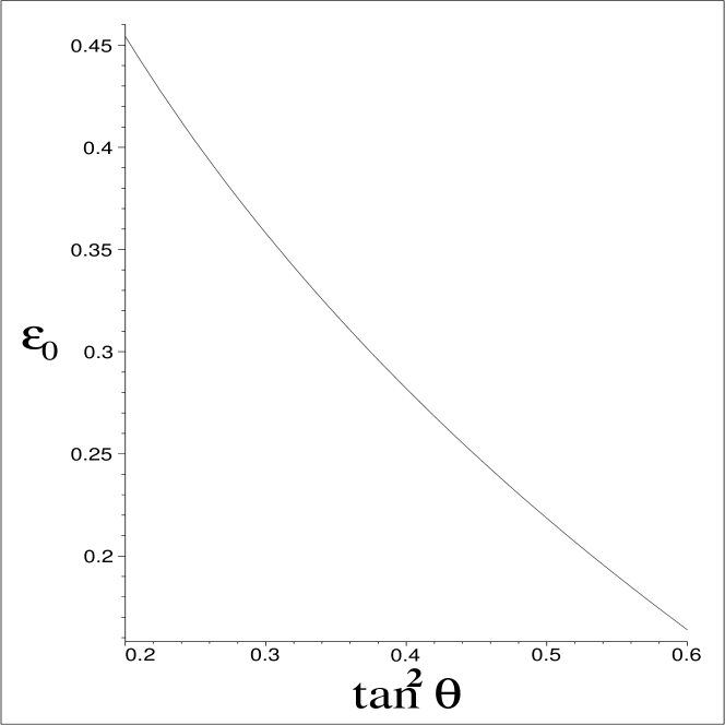
Figure 1: The dependence of $\epsilon_{0}=2EV_{0}/\Delta m^{2}$ on $\tan^{2}\theta$ obtained by setting the prefactor in eq. (55) equal to zero.

A ’good’ value of $\epsilon_{0}$ may come from the observation that the second order term in (53) is multiplied by the prefactor

$$(\cos 2\theta^{m}_{0}+\cos 2\theta^{\prime}_{0}-2\sin^{2}\theta-2\epsilon_{0}\sin^{2}2\theta^{m}_{0})\ .$$ (55)

Since $\epsilon_{0}$ is arbitrary, one may choose it such that this prefactor vanishes. In Fig.1 we show the $\tan^{2}\theta$ dependence of $\epsilon_{0}$ for which the prefactor vanishes.

In the limit $V\rightarrow 0$ the second, the third and the forth terms in (53) cancel each other ( up to $\epsilon_{0}^{3}$), and the probability reduces to $\sin^{2}\theta$.

IV Corrections due to three-neutrino mixing

In the standard parametrization the lepton mixing matrix is

$$U=O_{23}\,diag(1,1,e^{i\delta_{cp}})O_{13}\,diag(1,1,e^{-i\delta_{cp}})O_{12}=$$

$${\left(\!\!\!\!\begin{tabular}[]{ccc}$c_{13}c_{12}$&$c_{13}s_{23}$&$s_{13}e^{-i\delta_{cp}}$\\ $-s_{12}c_{23}-c_{12}s_{23}s_{13}e^{i\delta_{cp}}$&$c_{12}c_{23}-s_{12}s_{23}s_{13}e^{i\delta_{cp}}$&$c_{13}s_{23}$\\ $s_{12}s_{23}-c_{12}c_{23}s_{13}e^{i\delta_{cp}}$&$-c_{12}s_{23}-s_{12}c_{23}s_{13}e^{i\delta_{cp}}$&$c_{13}c_{23}$\end{tabular}\!\!\!\right)}$$ (59)

By a redefinition of the mixing matrix

$$U\to U\cdot diag(1,1,e^{i\delta_{cp}})$$ (60)

the Hamiltonian becomes real, i.e.

000000)​U0000fragmentsΔ𝑠000fragmentsΔ𝑎superscript𝑈†fragments 000000𝑈\displaystyle\left(\begin{tabular}[]{ccc}0&0&0\\ 0&$\Delta_{s}$&0\\ 0&0&$\Delta_{a}$\end{tabular}\right)+U^{\dagger}\left(\begin{tabular}[]{ccc}V&0&0\\ 0&0&0\\ 0&0&0\end{tabular}\right)U

$${\cal H} = \left(\begin{tabular}[]{ccc}0&0&0\\ 0&$\Delta_{s}$&0\\ 0&0&$\Delta_{a}$\end{tabular}\right)+U^{\dagger}\left(\begin{tabular}[]{ccc}V&0&0\\ 0&0&0\\ 0&0&0\end{tabular}\right)U$$ V00V00 (67)

$$= \left(\begin{tabular}[]{lll}$Vc^{2}_{13}c^{2}_{12}$&\ $Vc^{2}_{13}s_{12}c_{12}$&\ $Vc_{12}c_{13}s_{13}$\\ $Vc^{2}_{13}s_{12}c_{12}$&\ $\Delta_{s}+Vc^{2}_{13}s^{2}_{12}$&\ $Vs_{12}c_{13}s_{13}$\\ $Vc_{12}c_{13}s_{13}$&\ $Vs_{12}c_{13}s_{13}$&\ $\Delta_{a}+Vs^{2}_{13}$\end{tabular}\right),$$ (71)

where $\Delta_{s}\equiv\Delta m^{2}_{\odot}/2E$ and $\Delta_{a}\equiv\Delta m^{2}_{atm}/2E-\Delta_{s}$.

Thus we see that both the CP phase $\delta_{cp}$ and $\theta_{23}$ do not influence the propagation in matter (determined by the Hamiltonian). Also, since in (60) the first line does not contain $\delta_{cp}$ and $\theta_{23}$ these parameters disappear in the oscillations from $\nu_{e}$ to $\nu_{e}$, or from $\nu_{e}$ to mass eigenstates and vice versa. They manifest themselves only when one considers the flavor states $\nu_{\mu}$ or $\nu_{\tau}$.

These arguments are general and are valid in arbitrary matter density.

We now write the Hamiltonian in the form

$${\cal H}={\cal H}_{(3\nu)}^{0}+\Upsilon_{(3\nu)},$$ (72)

where

$${\cal H}_{(3\nu)}^{0}=\left(\begin{tabular}[]{ccc}0&0&0\\ 0&$\Delta_{s}^{m}$&0\\ 0&0&$\Delta_{a}^{m}$\end{tabular}\right)$$ (73)

and

$$\Upsilon_{(3\nu)}\!\!\! = \!\!{\cal H}\!-\!{\cal H}^{0}_{3\nu}\!+\!diag(0,\Delta_{s},\Delta_{a})-{V\!\!+\!\!\Delta_{s}\!\!+\!\!\Delta_{a}\!\!-\!\!\Delta_{s}^{m}\!\!\!\!-\!\!\Delta_{a}^{m}\over 3}I$$ (77)

$$=V\,c_{13}^{2}\left(\begin{tabular}[]{ccc}0&$\sin 2\theta_{12}/2$&$c_{12}s_{13}/c_{13}$\\ $\sin 2\theta_{12}/2$&0&$s_{12}s_{13}/c_{13}$\\ $c_{12}s_{13}/c_{13}$&$s_{12}s_{13}/c_{13}$&0\end{tabular}\right)\!+\!O(V^{2}).$$

$\Delta_{s}^{m}$ and $\Delta_{a}^{m}$ are the eigenvalues of the Hamiltonian in matter . In eq. (77) we have subtracted a term proportional to the unit matrix in order to make it traceless and thus convenient for a power expansion.

A straightforward calculation leads to the transition probabilities of the mass eigenstates to $\nu_{e}$:

$$P_{\nu_{1}\to\nu_{e}}\!\!\!\!\! = \!\!\!c_{13}^{2}c_{12}^{2}-{\sin^{2}2\theta_{12}\over 2}c_{13}^{4}\int_{x_{0}}^{x_{f}}\!\!\!\!\!dx\,V\sin\phi_{x\to x_{f}}$$ (78)

$$-2\,c_{12}^{2}c_{13}^{2}s_{13}^{2}\int_{x_{0}}^{x_{f}}\!\!\!\!\!dx\,V\sin\psi_{x\to x_{f}},$$

$$P_{\nu_{2}\to\nu_{e}}\!\!\!\!\! = \!\!\!c_{13}^{2}s_{12}^{2}+{\sin^{2}2\theta_{12}\over 2}c_{13}^{4}\int_{x_{0}}^{x_{f}}\!\!\!\!\!dx\,V\sin\phi_{x\to x_{f}}$$ (79)

$$-2\,s_{12}^{2}c_{13}^{2}s_{13}^{2}\int_{x_{0}}^{x_{f}}\!\!\!\!\!dx\,V\sin(\psi_{x\to x_{f}}\!\!\!-\!\phi_{x\to x_{f}}),$$

$$P_{\nu_{3}\to\nu_{e}}\!\!\!\!\! = \!\!\!s_{13}^{2}+2\,c_{12}^{2}c_{13}^{2}s_{13}^{2}\int_{x_{0}}^{x_{f}}\!\!\!\!\!dx\,V\sin\psi_{x\to x_{f}}$$ (80)

$$+2\,s_{12}^{2}c_{13}^{2}s_{13}^{2}\int_{x_{0}}^{x_{f}}\!\!\!\!\!dx\,V\sin(\psi_{x\to x_{f}}\!\!\!-\!\phi_{x\to x_{f}}),$$

where

$$\phi_{a\to b}=\int_{a}^{b}\Delta_{s}^{m}(x)\,dx\ ,~{}~{}~{}~{}~{}\psi_{a\to b}=\int_{a}^{b}\Delta_{a}^{m}(x)\,dx\ .$$ (81)

The function $\sin\psi_{x\to x_{f}}$ oscillates $\Delta_{a}^{m}/\Delta_{s}^{m}\simeq\Delta m^{2}_{atm}/\Delta m^{2}_{\odot}$ times faster than $\sin\phi_{x\to x_{f}}$. Thus, the corresponding integral is roughly $\Delta m^{2}_{atm}/\Delta m^{2}_{\odot}$ times smaller than the one which contains the phase $\phi$; furthermore, it has a prefactor $s_{13}^{2}$. Therefore we get to a good approximation

$$P_{\nu_{1}\to\nu_{e}}\!\!\!\!\! = \!\!\!c_{13}^{2}c_{12}^{2}-{\sin^{2}2\theta_{12}\over 2}c_{13}^{4}\int_{x_{0}}^{x_{f}}\!\!\!\!\!dx\,V\sin\phi_{x\to x_{f}},$$ (82)

$$P_{\nu_{2}\to\nu_{e}}\!\!\!\!\! = \!\!\!c_{13}^{2}s_{12}^{2}+{\sin^{2}2\theta_{12}\over 2}c_{13}^{4}\int_{x_{0}}^{x_{f}}\!\!\!\!\!dx\,V\sin\phi_{x\to x_{f}},$$ (83)

$$P_{\nu_{3}\to\nu_{e}}\!\!\!\!\! \simeq \!\!\!s_{13}^{2}.$$ (84)

These results may be also obtained from eq. (71) Akhmedov:2004rq (see ohl for some earlier discussion). If $\Delta_{a}\gg\Delta_{s}\gg V$ and $s_{13}\ll 1$, the third neutrino decouples and one arrives at the two neutrino propagation problem in matter with potential $V\to Vc_{13}^{2}$ and mixing angle $\theta_{12}$. Following the procedure of section II and using the full mixing matrix $U\,diag(1,1,e^{i\delta_{cp}})$ we easily recover eqs. (82) -(84).

V Conclusion

Motivated by the large mixing MSW solution to the solar neutrino we have developed a simple formulation of the earth matter effects on low energy neutrino beams. Following Ioannisian:2004jk , we derive an expansion for the neutrino transitions in terms of the parameter

$$\epsilon(x)\equiv{2EV(x)\over\Delta m^{2}}$$

to second order. By choosing a convenient constant average value for the neutrino potential as starting point, the precision can be substantially improved and it is possible to reach an accuracy of a few percents even for energies near $70-80$ MeV. The effective expansion parameter is a simple integral in eq. (41) (or eq. (54)) together with eq. (20)) which can be done numerically. The expansion allows for a convenient quantitative discussion of various physical effects such as the attenuation effect to the remote structures of the density profile or the effect of energy resolution of detectors. We also consider the case of three-neutrino mixing.

The work of A.N.I. was supported by the Swiss National Science Foundation (SNF). A.N.I. thanks the University of Zürich for hospitality.

References

• (1) L. Wolfenstein, Phys. Rev. D 17, 2369 (1978); L. Wolfenstein, in ”Neutrino-78”, Purdue Univ. C3, (1978).
• (2) S. P. Mikheyev and A. Yu. Smirnov, ’86 Massive Neutrinos in Astrophysics and in Particle Physics, proceedings of the Sixth Moriond Workshop, edited by O. Fackler and J. Tr$\hat{a}$n Thanh V$\hat{a}$n (Editions Frontières, Gif-sur-Yvette, 1986), p. 355.
• (3) J. Bouchez et. al., Z. Phys. C32, 499 (1986); M. Cribier et. al., Phys. Lett. B 182, 89 (1986); E. D. Carlson, Phys. Rev. D34, 1454 (1986).
• (4) A.J. Baltz and J. Weneser, Phys. Rev. D35, 528 (1987).
• (5) S. P. Mikheyev and A. Yu. Smirnov, Sov. Phys. Usp. 30 (1987) 759; L. Cherry and K. Lande, Phys. Rev D 36 3571 (1987); S. Hiroi, H. Sakuma, T. Yanagida, M. Yoshimura, Phys. Lett. B198 403, (1987) and Prog. Theor. Phys. 78 1428, (1987); A. Dar, A. Mann, Y. Melina and D. Zajfman, Phys. Rev D35, 3607 (1987); A. J. Baltz and J. Weneser, Phys. Rev. D37, 3364 (1988); M. Spiro and D. Vignaud, Phys. Lett. B 242 297 (1990).
• (6) J.N. Bahcall, P.I. Krastev, Phys. Rev. C56: 2839 (1997).
• (7) E. Lisi and D. Montanino, Phys. Rev. D56, 1792 (1997).
• (8) E.K. Akhmedov, Nucl. Phys. B538(1999)25.
• (9) M. Maris, S.T. Petcov, Phys. Lett. B457:319, (1999).
• (10) M. C. Gonzalez-Garcia, C. Pena-Garay, A. Yu. Smirnov, Phys. Rev. D63:113004, (2001).
• (11) G. L. Fogli, E. Lisi, A. Marrone, D. Montanino and A. Palazzo, Phys. Rev. D 66, 053010 (2002).
• (12) Lian-You Shan, Xin-Min Zhang, Phys. Rev. D65:113011, (2002).
• (13) M. B. Smy et al., Super-Kamiokande Collaboration, Phys. Rev. D69(2004) 011104.
• (14) M. Blennow, T. Ohlsson, H. Snellman Phys. Rev. D69:073006, (2004).
• (15) A. S. Dighe, A. Yu. Smirnov Phys. Rev. D62:033007, (2000).
• (16) C. Lunardini, A.Yu. Smirnov, Nucl. Phys. B616: 307,2001.
• (17) V. D. Barger, D. Marfatia, K. Whisnant, B.P. Wood, Phys. Rev. D64:073009, (2001).
• (18) K. Takahashi and K. Sato, Phys.Rev. D 66, 033006 (2002).
• (19) A. S. Dighe, M. T. Keil, G. G. Raffelt JCAP 0306:006, (2003).
• (20) A. N. Ioannisian, A. Yu. Smirnov, hep-ph/0201012.
• (21) M. Lindner, T. Ohlsson, R. Tomas, W. Winter, Astropart. Phys. 19 (2003) 755.
• (22) A.S. Dighe, M. Kachelriess, G.G. Raffelt, R. Tomas, JCAP 0401:004, (2004).
• (23) A. N. Ioannisian and A. Y. Smirnov, arXiv:hep-ph/0404060.
• (24) P.C. de Holanda, Wei Liao, A. Yu. Smirnov, hep-ph/0404042.
• (25) E. K. Akhmedov, M. A. Tortola and J. W. F. Valle, JHEP 0405, 057 (2004). In the original version of the paper (hep-ph/0404083 v.1) the ’wrong’ vacuum phase has been derived and the correct oscillation phase has been introduced on the “heuristic” ground. Its derivation is given in later journal version.