Abstract

We study the properties of light mesons in the scalar, pseudo-scalar, and vector channels within the light-front quantization, by using the (one flavor) Nambu–Jona-Lasinio model with vector interaction. After taking into account the effects of chiral symmetry breaking, we derive the bound-state equation in each channel in the large $N$ limit ($N$ is the number of colors), which means that we consider the lowest $q\bar{q}$ Fock state with the constituent quark and antiquark. By solving the bound-state equation, we simultaneously obtain a mass and a light-cone (LC) wavefunction of the meson. While we reproduce the previous results for the scalar and pseudo-scalar mesons, we find that, for a vector meson, the bound-state equations for the transverse and longitudinal polarizations look different from each other. However, eventually after imposing a cutoff which is invariant under the parity and boost transformations, one finds these two are identical, giving the same mass and the same (spin-independent) LC wavefunction. When the vector interaction becomes larger than a critical value, the vector state forms a bound state, whose mass decreases as the interaction becomes stronger. While the LC wavefunction of the pseudo-scalar meson is broadly distributed in longitudinal momentum ($x$) space, that of the vector meson is squeezed around $x=1/2$.

1 Introduction

Understanding the structure of light mesons at low energies is one of the most difficult problems in QCD, which requires nonperturbative studies about three entangled issues: chiral symmetry breaking, confinement of quarks and gluons, and relativistic bound-state physics. The light-front (LF) quantization is now widely accepted as the most transparent formalism for the third issue, the relativistic bound-state physics [1], and thus, if the other two are also accommodated by the LF formalism, then it can be a very powerful tool for the problem. This expectation has been shared by many people with continuous interests and efforts in the LF formalism. The present paper is one of such attempts towards establishing the methods for describing the chiral symmetry breaking on the LF.

The advantage of the LF formalism in treating the relativistic bound-state physics is closely related to the fact that the vacuum in this formalism is very simple, and is actually the Fock vacuum itself even for an interacting system. Roughly speaking, this property allows us to construct a Hamiltonian equation $H_{\rm LC}\left.\left|\alpha\right.\right\rangle=E\left.\left|\alpha\right.\right\rangle$ with only a few Fock states just like in the Tamm-Dancoff approximation. By solving this equation, one can simultaneously find the wavefunction of each Fock state and the eigen-value (mass) of the eigen state. This is certainly the unique merit of the LF formalism. On the other hand, the other two properties, chiral symmetry breaking and confinement, are usually believed to be related to the nontrivial vacuum structure. This does not mean that the LF quantization is not useful for the problem mentioned above, but rather means that one has to discover new ways of formulating the physics of confinement and chiral symmetry breaking within the context of the LF quantization. This motivated several efforts towards setting up the problems in QCD, and actually many new interesting ideas and techniques were generated in such activities (see for example, Ref. [2]). However, we have not reached at a satisfactory description for these problems.

Meanwhile, there has been considerable progress in describing the spontaneous symmetry breaking in scalar theories within the LF quantization [1]. It was recognized that the longitudinal zero mode of a scalar field plays a crucial rôle. The scalar zero mode is not a dynamical mode in the LF quantization, and subject to a non-linear constraint equation, called the zero-mode constraint. Spontaneous symmetry breaking can be achieved through the nonperturbative solution to the zero-mode constraint, which brings in a nonzero vacuum expectation value to the scalar field. Moreover, based on the analogies with such achievements, even the chiral symmetry breaking in simple fermionic models (without gauge fields) were described within the LF quantization [3, 4] (See Ref. [5] for a review about these approaches based on the canonical LF quantization. For an alternative treatment based on the path-integral approach, see Ref. [6]). Therefore, the region governed by the LF formalism is now slowly expanding, while the chiral symmetry breaking in real QCD is still not under control (see, however, Ref. [7]).

Indeed, within the Nambu–Jona-Lasinio (NJL) model, which is sometimes considered as an effective theory of QCD [8, 9], it has been found that, still with the trivial Fock vacuum, chiral symmetry breaking is described in such a way that one selects an appropriate Hamiltonian depending on the phases of the symmetry [4]. In the NJL model, different Hamiltonians are originated from different solutions to a constraint equation, which exists only in the LF formalism. The ”bad” component of the spinor is not a dynamical variable and is subject to a constraint equation like the zero mode in scalar theories. This ”fermionic constraint” is nonlinear in the NJL model and leads to the ”gap equation” for the chiral condensate. When the coupling constant is larger than the critical value, the gap equation has a non-zero solution even in the chiral limit. This means that the fermionic constraint allows for ”symmetric” and ”broken” solutions corresponding to those of the gap equation. If one selects the ”broken” solution, and substituting it to the canonical Hamiltonian, one obtains the ”broken” Hamiltonian. This governs the dynamics in the broken phase and is completely different from the Hamiltonian with the ”symmetric” solution. In Ref. [4], two of us solved the fermionic constraint by using the $1/N$ expansion, and obtained the Hamiltonians in both symmetric and broken phases. They also solved the bound-state equations for the scalar and pseudo-scalar mesons and obtained their light-cone (LC) wavefunctions and masses, as well as the PCAC and Gell-Mann, Oakes, Renner (GOR) relations.

The main objective of the present paper is to extend the analysis of Ref. [4] to the vector channel by using a similar model, and investigate the properties of a vector meson. A part of the results was already reported without detailed derivations [10]. Thus, in this paper, we will re-derive all the results in a self-contained way as much as possible. We will also present a slightly deeper understanding of the properties of scalar and pseudo-scalar mesons.

It will be helpful to briefly summarize the main results of the present paper. After lengthy calculations, we are able to derive $q\bar{q}$ bound-state equations in the pseudo-scalar ($\pi$), scalar ($\sigma$), and vector (V) channels. By solving these equations, we will eventually obtain the LC wavefunctions and masses of the mesons. Remarkably, it turns out that, due to the contact interaction of the NJL model, the spin-independent part of the LC wavefunction for each meson ($i=\pi,\,\sigma,\,$V) has a very simple form (see Eq. (5.1)):

$$\phi_{i}(x,k_{\perp})\propto\frac{1}{m_{i}^{2}-\frac{k_{\perp}^{2}+M^{2}}{x(1-x)}},$$

where $x$ is the fraction of longitudinal momentum carried by a quark, $k_{\perp}$ is the relative transverse momentum between the quark and the antiquark, $M$ is the constituent quark mass, and $m_{i}$ is the mass of the meson $i$. This result is common for all the mesons discussed in the paper. The difference among the LC wavefunctions is visible only through the value of the meson mass $m_{i}$. For example, in the chiral limit, we will find a relation $0=m_{\pi}<m_{\rm V}<m_{\sigma}=2M$. Namely, the LC wavefunction of the pseudo-scalar has a broad distribution in $x$ space, while that of the scalar meson is rather peaked around the mean value $x=1/2$, and the vector meson comes in between these two (see Fig. 3).

The paper is organized as follows. In the next section, we will define the NJL model with the vector interaction. The vector interaction is added to have a bound state in the vector channel. We also show the explicit form of the fermionic constraint of this model. In Sect. 3, we solve the fermionic constraint by using the $1/N$ expansion, and derive the LC Hamiltonian to the first nontrivial order. This allows us to derive the bound-state equations of light mesons, which is discussed in Sect. 4. To the leading nontrivial order of the $1/N$ expansion, mesons are described by a quark-antiquark state, and the bound-state equations can be restricted to the lowest $q\bar{q}$ Fock states. In Sect. 5, we solve the bound-state equations in scalar, pseudo-scalar, and vector channels, and obtain the masses of mesons and the LC wavefunctions as already discussed above. We will show that, when we treat the bound-state equations, we have to be extremely careful about the regularization scheme. Otherwise, the equations for transverse and longitudinal polarizations of the vector meson look differently. Summary and discussions are given in Sect. 6. Some detailed calculations, as well as the notation we use are presented in Appendix.

2 The model

In this section, we define the NJL model we use, and discuss its particular properties when it is quantized on the light front. We also clarify our strategy which we take in the present paper.

2.1 Nambu–Jona-Lasinio model with vector interaction

The simplest NJL model is given by

$${\cal L}_{\rm NJL} = \bar{\Psi}_{a}(i\partial\!\!\!/-m_{0})\Psi_{a}+{\cal L}_{\rm S}\,,$$

$${\cal L}_{\rm S} \equiv \frac{G_{\rm S}}{2}\left[(\bar{\Psi}_{a}\Psi_{a})^{2}+(\bar{\Psi}_{a}i\gamma_{5}\Psi_{a})^{2}\right]\,,$$ (2.1)

where $\Psi_{a}$ is a spinor in the fundamental representation of ”color” SU($N$) group ($a$ is a color index: $a=1,\cdots,N$). The scalar interaction ${\cal L}_{\rm S}$ is constructed as ”color” singlet. In what follows, we suppress the color index $a$ for notational simplicity, which however does not cause any confusion because, throughout the paper except this section, we always treat color singlet objects (i.e., bilocal operators to be defined below). We consider the case with one flavor for simplicity. Generalization to the case with multi flavors, which is necessary for phenomenological applications, is more complicated but is straightforward. Recently, this model was analyzed in the light-front quantization by two of the authors [4] (see also Ref. [3]) and they computed masses and light-cone wavefunctions of scalar and pseudo-scalar mesons to the first nontrivial order of the $1/N$ expansion. One can of course apply the same procedure for vector states, but we know that the simplest NJL model defined by ${\cal L}_{\rm NJL}$ does not allow for a bound state in the vector channel [8, 11]. Vector states start to bind if one adds the vector interaction so that the attractive force between a quark and an antiquark in the vector channel becomes stronger. Therefore, we include the vector interaction minimally by adding the following interaction:

$${\cal L}_{\rm V}=-\frac{G_{\rm V}}{2}\left[(:\bar{\Psi}\gamma_{\mu}\Psi:)^{2}+(:\bar{\Psi}\gamma_{\mu}\gamma_{5}\Psi:)^{2}\right].$$ (2.2)

Notice that this interaction does not change the nontrivial ”vacuum structure” (more precisely, the value of chiral condensate) which is caused by ${\cal L}_{\rm S}$. This is because we have taken the normal order in (2.2) which is defined with respect to the Fourier modes of the fermion field (see below for the details). On the other hand, the bound-state equations for scalar and pseudo-scalar mesons will be modified due to the vector interaction.

It would be very helpful to summarize here the issues to be discussed in the present paper and our strategy against them. There are mainly three issues: (i) chiral symmetry breaking, (ii) $q\bar{q}$ bound states in the scalar and pseudo-scalar channels, and (iii) $q\bar{q}$ bound states in the vector channel. Below we briefly explain the roles played by the interactions ${\cal L}_{\rm S}$ and ${\cal L}_{\rm V}$ for these problems. The precise meaning of all the procedures and approximations will be clarified in the forthcoming sections.

1. Chiral symmetry breaking is generated by the interaction ${\cal L}_{\rm S}$, and is not affected by the inclusion of the vector interaction ${\cal L}_{\rm V}$ (by construction) to the leading order of the $1/N$ expansion.

2. Bound states in the scalar and pseudo-scalar channels are possible in the presence of the scalar interaction ${\cal L}_{\rm S}$. Thus, in this paper, we will study them with the Lagrangian (2.1). Although the vector interaction ${\cal L}_{\rm V}$ will modify the scalar and pseudo-scalar bound states, we shall ignore the effects of ${\cal L}_{\rm V}$ expecting that the scalar interaction ${\cal L}_{\rm S}$ gives the dominant effect.

3. Bound states in the vector channel are not formed with ${\cal L}_{\rm S}$ alone, but can exist with the help of ${\cal L}_{\rm V}$. Thus, to study the bound-state physics in the vector channel, we need to include the effects of ${\cal L}_{\rm V}$. In the actual calculation, we will take the leading contribution of the eigen-value equation with respect to $G_{\rm V}$ which is enough to form a bound state.

Therefore, in the following analysis, inclusion of the vector interaction (2.2) is only relevant for the bound-state physics of the vector state.

2.2 A constraint equation for the bad spinor component

One of the main sources of complexities in the light-front quantization is the presence of constraint equations which appear only when we treat the light-cone variable $x^{+}$ as the evolution time. In a system involving a fermion field, one always has a constraint equation for the ”bad” component of the spinor $\psi_{-}$ (where $\psi_{\pm}\equiv\Lambda_{\pm}\Psi=\frac{1}{2}\gamma^{\mp}\gamma^{\pm}\Psi$ and $\psi_{+}$ is refereed to as ”good”, see Appendix A for our notations) because the kinetic term $i\bar{\Psi}\partial\!\!\!/\Psi$ is expressed as $i\psi_{+}^{\dagger}\partial_{+}\psi_{+}+i\psi_{-}^{\dagger}\partial_{-}\psi_{-}+\cdots$ and $\partial_{-}$ is now a spatial derivative $\partial_{-}=\partial/\partial x^{-}$. This constraint equation which we call the ”fermionic constraint”, is easily obtained if we multiply the Euler-Lagrange equation by the projector $\Lambda_{+}$ from the left ($\Lambda_{+}\gamma^{-}\partial_{-}\Psi=\gamma^{-}\Lambda_{-}\partial_{-}\Psi=\gamma^{-}\partial_{-}\psi_{-}$):

$$\Lambda_{+}\left[(i\partial\!\!\!/-m_{0})\Psi+\frac{\delta}{\delta\bar{\Psi}}~{}({\cal L}_{\rm S}+{\cal L}_{\rm V})\right]=0\,.$$

Without the vector interaction, the fermionic constraint takes a rather simple form:

$$i\partial_{-}\,\psi_{-}=\frac{1}{2}\,\left(i\gamma^{j}_{\perp}\partial_{\perp j}+m_{0}\right)\gamma^{+}\psi_{+}-\frac{G_{\rm S}}{2}\Big{[}\gamma^{+}\psi_{+}(\bar{\psi}_{+}\psi_{-}+\bar{\psi}_{-}\psi_{+})-i\gamma_{5}\gamma^{+}\psi_{+}(\bar{\psi}_{+}i\gamma_{5}\psi_{-}+\bar{\psi}_{-}i\gamma_{5}\psi_{+})\Big{]}.$$

(2.3)

While this is just a first order differential equation, the term coming from the interaction makes the analysis difficult. Still, in a classical level, this equation can be exactly solved [4], which helps to understand properties of the ”chiral transformation” on the light front that is different from the ordinary one because the chiral transformation is imposed only on the dynamical (”good”) component [5]. But, as was discussed in Ref. [4], in order to describe the symmetry breaking, we need to solve the fermionic constraint in a quantum level, which we will indeed do in the next section. It should be noticed that, in the quantum theory, the operator ordering must be specified, though it is a priori not known. Thus in Ref. [4], they defined the quantum theory by the above operator-ordering. Namely, $\psi_{+}$ comes to the left of color singlet operators such as $\bar{\psi}_{+}\psi_{-}$ or $\bar{\psi}_{+}i\gamma_{5}\psi_{-}$. Since this operator ordering correctly reproduces physics of the chiral symmetry breaking, we adopt the same operator ordering in the present paper.

With the vector interaction included, the corresponding fermionic constraint becomes terribly complicated, while its structure (as a differential equation) is the same as Eq. (2.3). We show its explicit form for later convenience:

$$i\partial_{-}\psi_{-}\!\! = \!\!\frac{1}{2}\left(i\gamma^{i}_{\perp}\partial_{\perp i}+m_{0}\right)\gamma^{+}\psi_{+}-\frac{G_{\rm S}}{2}\Big{[}\gamma^{+}\psi_{+}(\bar{\psi}_{+}\psi_{-}+\bar{\psi}_{-}\psi_{+})-i\gamma_{5}\gamma^{+}\psi_{+}(\bar{\psi}_{+}i\gamma_{5}\psi_{-}+\bar{\psi}_{-}i\gamma_{5}\psi_{+})\Big{]}$$ (2.4)

$$+\,G_{\rm V}\,\Big{[}\psi_{-}(:\bar{\psi}_{+}\gamma^{+}\psi_{+}:)+\gamma_{5}\psi_{-}(:\bar{\psi}_{+}\gamma^{+}\gamma_{5}\psi_{+}:)\Big{]}$$

$$+\,\frac{G_{\rm V}}{2}\left[\gamma^{i}_{\perp}\gamma^{+}\psi_{+}:\left\{\bar{\psi}_{+}\gamma^{i}_{\perp}\psi_{-}+\bar{\psi}_{-}\gamma^{i}_{\perp}\psi_{+}\right\}:-\gamma_{\perp}^{i}\gamma_{5}\gamma^{+}\psi_{+}:\left\{\bar{\psi}_{+}\gamma^{i}_{\perp}\gamma_{5}\psi_{-}+\bar{\psi}_{-}\gamma^{i}_{\perp}\gamma_{5}\psi_{+}\right\}:\right].\hskip 25.60747pt$$

Here we have followed the same operator ordering as in Eq. (2.3). This equation only makes sense in the quantum level because we have already taken the normal order.

2.3 Quantization

Since the bad component of the spinor is not an independent degree of freedom, the quantization condition is imposed only on the good component. From Dirac’s procedure, one finds the following anti-commuting relations:

$$\left\{\psi_{+\alpha}(\mbox{\boldmath{$x$}}),\,\psi_{+\beta}^{\dagger}(\mbox{\boldmath{$y$}})\right\}_{x^{+}=y^{+}}=\frac{1}{\sqrt{2}}(\Lambda_{+})_{\alpha\beta}\ \delta(\mbox{\boldmath{$x$}}-\mbox{\boldmath{$y$}})\,,$$ (2.5)

$$\Big{\{}\psi_{+\alpha}(\mbox{\boldmath{$x$}}),\,\psi_{+\beta}(\mbox{\boldmath{$y$}})\Big{\}}_{x^{+}=y^{+}}=\left\{\psi_{+\alpha}^{\dagger}(\mbox{\boldmath{$x$}}),\,\psi_{+\beta}^{\dagger}(\mbox{\boldmath{$y$}})\right\}_{x^{+}=y^{+}}=0\,,$$ (2.6)

where $\delta(\mbox{\boldmath{$x$}}-\mbox{\boldmath{$y$}})\equiv\delta(x^{-}-y^{-})\,\delta^{(2)}(x_{\perp}-y_{\perp}).$ The mode expansion of the field is given by

$$\psi_{+}(\mbox{\boldmath{$x$}})=\,\int\frac{[d\mbox{\boldmath{$p$}}]}{\left(2\pi\right)^{3/2}}\,\frac{1}{\sqrt{2p^{+}}}\sum_{s=\pm}\left[\,b(\mbox{\boldmath{$p$}},s)\,u_{+}(\mbox{\boldmath{$p$}},s)\,{\rm e}^{-ip\cdot x}\,+\,d^{\dagger}(\mbox{\boldmath{$p$}},s)\,v_{+}(\mbox{\boldmath{$p$}},s)\,{\rm e}^{ip\cdot x}\,\right],$$

where we have introduced notation for the integration

$$\int[d\mbox{\boldmath{$p$}}]\equiv\int_{0}^{\infty}dp^{+}\int_{-\infty}^{\infty}d^{2}p_{\perp}\,,$$

and $u_{+}(\mbox{\boldmath{$p$}},s)$ and $v_{+}(\mbox{\boldmath{$p$}},s)$ are the good components of the solutions (with spin $s$) to the free Dirac equation, i.e., $u_{+}\equiv\Lambda_{+}u$ and $v_{+}\equiv\Lambda_{+}v$ (for more details, see Appendix B). Notice that the longitudinal momentum $p^{+}$ takes only positive values because of the special property of the dispersion relation on the light front $p^{-}=(p_{\perp}^{2}+m^{2})/2p^{+}>0$. The operators $b(\mbox{\boldmath{$p$}},s)$ for quarks and $d(\mbox{\boldmath{$p$}},s)$ for anti-quarks satisfy the anti-commutation relations:

$$\left\{b(\mbox{\boldmath{$p$}},s),\,b^{\dagger}(\mbox{\boldmath{$p$}}^{\prime},s^{\prime})\right\}=\left\{d(\mbox{\boldmath{$p$}},s),\,d^{\dagger}(\mbox{\boldmath{$p$}}^{\prime},s^{\prime})\right\}=\delta_{ss^{\prime}}\,\delta(\mbox{\boldmath{$p$}}-\mbox{\boldmath{$p$}}^{\prime}),$$ (2.7)

and zeros for other combinations. The normal order in Eq. (2.4) is defined with respect to these operators.

3 Fermionic constraints and LC Hamiltonians

Here we solve the fermionic constraint in the quantum theory, and compute the LC Hamiltonian which is one of the necessary ingredients for deriving the bound-state equations. While the whole procedure, with the vector interaction included, is really tedious, it is straightforward and essentially the same as in the case without the vector interaction which was recently achieved in Ref. [4]. Thus, in this section, we first discuss the case without the vector interaction in order to demonstrate the methods we use. The presentation is basically along the previous analysis of Ref. [4], but we here adopt the spinor basis for the mode expansion (2.3) (cf. instead of a simple Fourier expansion, Eq. (3.2) in Ref. [4]) and do not use any specific representations of the $\gamma$ matrices, both of which are much more convenient for the extension to the case with vector interaction. In order to avoid too much technicalities, but still to keep the paper self-contained as much as possible, we put some of the details aside to Appendix D. The involved case with vector interaction follows after this, with emphasis only on the differences coming from the inclusion of the vector interactions. Notice also that the analysis without the vector interaction can be applied to the scalar and pseudo-scalar mesons since we simply ignore the effects of vector interaction in these channels.

3.1 The case without vector interaction as a warm-up

3.1.1 Solving the fermionic constraint in bilocal form

It was found in Ref. [4] that one can systematically solve the fermionic constraint by using the $1/N$ expansion after rewriting it with respect to color singlet bilocal operators. The $1/N$ expansion of the bilocal operator equations is made possible by use of the boson expansion method, which has been known as a standard technique in many body physics, but was only recently applied to the light-front field theories in Ref. [12]. The basic quantity is defined by a color singlet bilocal operator of the good component at different space points and at the same LC time:

$${\sf M}_{\alpha\beta}(\mbox{\boldmath{$x$}},\mbox{\boldmath{$y$}})\equiv\sqrt{2}\,\psi_{+\alpha}^{{\dagger}}(\mbox{\boldmath{$x$}})\,\psi_{+\beta}(\mbox{\boldmath{$y$}})\,,$$ (3.1)

where $\mbox{\boldmath{$x$}}=(x^{-},x_{\perp}^{i})$ and $\alpha,\,\beta$ are the Dirac indices, and the color indices are suppressed. We further introduce bilocal operators of scalar (${\sf S}$) and pseudo-scalar (${\sf P}$) as follows:

$${\sf S}_{\rm R}(\mbox{\boldmath{$x$}},\mbox{\boldmath{$y$}}) \equiv \bar{\Psi}(\mbox{\boldmath{$x$}})\Lambda_{-}\Psi(\mbox{\boldmath{$y$}})\,+\,{\rm h.c.},$$ (3.2)

$${\sf P}_{\rm R}(\mbox{\boldmath{$x$}},\mbox{\boldmath{$y$}}) \equiv \bar{\Psi}(\mbox{\boldmath{$x$}})\Lambda_{-}(i\gamma_{5})\Psi(\mbox{\boldmath{$y$}})\,+\,{\rm h.c.},$$ (3.3)

where h.c. is the hermitian conjugate and the subscript ”R” implies that it is the ”real” part (later we will define the ”imaginary” part when we discuss the case with vector interaction). Notice that these bilocal operators reduce to the scalar and pseudo-scalar operators at the same space-time point: ${\sf S}_{\rm R}(\mbox{\boldmath{$x$}},\mbox{\boldmath{$x$}})=\bar{\Psi}(\mbox{\boldmath{$x$}})\Psi(\mbox{\boldmath{$x$}})$ and ${\sf P}_{\rm R}(\mbox{\boldmath{$x$}},\mbox{\boldmath{$x$}})=\bar{\Psi}(\mbox{\boldmath{$x$}})i\gamma_{5}\Psi(\mbox{\boldmath{$x$}})$. Notice also that these quantities depend upon the bad component of the spinor $\psi_{-}$ and thus are not known until we solve the fermionic constraint. In other words, once we rewrite the fermionic constraint (2.3) with respect to the bilocal operators, they can be interpreted as the constraint equations for these unknown bilocal operators. In particular, the equations for ${\sf S}_{\rm R}$ and ${\sf P}_{\rm R}$ form a closed set of equations. Indeed, one obtains in momentum space

$$q^{+}{\sf S}_{\rm R}(\mbox{\boldmath{$p$}},\mbox{\boldmath{$q$}}) = \frac{1}{2}\left(\gamma^{i}q_{\perp}^{i}+m_{0}\right)_{\alpha\beta}\Big{(}{\sf M}_{\alpha\beta}(\mbox{\boldmath{$p$}},\mbox{\boldmath{$q$}})-{\sf M}_{\alpha\beta}(\mbox{\boldmath{$q$}},\mbox{\boldmath{$p$}})\Big{)}$$ (3.4)

$$-\,\frac{G_{\rm S}}{2}\int\frac{d^{3}\mbox{\boldmath{$k$}}\,d^{3}\mbox{\boldmath{$\l$}}}{(2\pi)^{3}}\left\{{\sf M}_{\alpha\beta}(\mbox{\boldmath{$p$}},\mbox{\boldmath{$q$}}-\mbox{\boldmath{$k$}}-\mbox{\boldmath{$\l$}})\Big{(}{\sf S}_{\rm R}+i\gamma_{5}\,{\sf P}_{\rm R}\Big{)}_{\alpha\beta}(\mbox{\boldmath{$k$}},\mbox{\boldmath{$\l$}})\right.$$

$$\hskip 71.13188pt\left.-\,\Big{(}{\sf S}_{\rm R}-i\gamma_{5}\,{\sf P}_{\rm R}\Big{)}_{\alpha\beta}(\mbox{\boldmath{$k$}},\mbox{\boldmath{$\l$}})\,{\sf M}_{\alpha\beta}(\mbox{\boldmath{$q$}}-\mbox{\boldmath{$k$}}-\mbox{\boldmath{$\l$}},\mbox{\boldmath{$p$}})\right\}\,,$$

$$q^{+}{\sf P}_{\rm R}(\mbox{\boldmath{$p$}},\mbox{\boldmath{$q$}}) = -\,\frac{1}{2}\left\{(i\gamma_{5})(\gamma^{i}q_{\perp}^{i}+m_{0})\right\}_{\alpha\beta}{\sf M}_{\alpha\beta}(\mbox{\boldmath{$p$}},\mbox{\boldmath{$q$}})\,-\,\frac{1}{2}\left\{(\gamma^{i}q_{\perp}^{i}+m_{0})(i\gamma_{5})\right\}_{\alpha\beta}{\sf M}_{\alpha\beta}(\mbox{\boldmath{$q$}},\mbox{\boldmath{$p$}})$$ (3.5)

$$+\,\frac{G_{\rm S}}{2}\int\frac{d^{3}\mbox{\boldmath{$k$}}\,d^{3}\mbox{\boldmath{$\l$}}}{(2\pi)^{3}}\left\{{\sf M}_{\alpha\beta}(\mbox{\boldmath{$p$}},\mbox{\boldmath{$q$}}-\mbox{\boldmath{$k$}}-\mbox{\boldmath{$\l$}})\Big{(}i\gamma_{5}\,{\sf S}_{\rm R}-{\sf P}_{\rm R}\Big{)}_{\alpha\beta}(\mbox{\boldmath{$k$}},\mbox{\boldmath{$\l$}})\right.$$

$$\hskip 71.13188pt\left.+\,\Big{(}i\gamma_{5}\,{\sf S}_{\rm R}+{\sf P}_{\rm R}\Big{)}_{\alpha\beta}(\mbox{\boldmath{$k$}},\mbox{\boldmath{$\l$}})\,{\sf M}_{\alpha\beta}(\mbox{\boldmath{$q$}}-\mbox{\boldmath{$k$}}-\mbox{\boldmath{$\l$}},\mbox{\boldmath{$p$}})\right\}~{},$$

where we have used short-hand notations like $({\sf S}_{\rm R}(\mbox{\boldmath{$p$}},\mbox{\boldmath{$q$}}))_{\alpha\beta}\equiv\delta_{\alpha\beta}\,{\sf S}_{\rm R}(\mbox{\boldmath{$p$}},\mbox{\boldmath{$q$}})$, $({\sf S}_{\rm R}+i\gamma_{5}\,{\sf P}_{\rm R})_{\alpha\beta}(\mbox{\boldmath{$k$}},\mbox{\boldmath{$\l$}})\equiv({\sf S}_{\rm R}(\mbox{\boldmath{$k$}},\mbox{\boldmath{$\l$}})+i\gamma_{5}\,{\sf P}_{\rm R}(\mbox{\boldmath{$k$}},\mbox{\boldmath{$\l$}}))_{\alpha\beta},$ etc, and the momentum integration is from $-\infty$ to $\infty$ (even for longitudinal momenta), which follows from our definition of the Fourier transformation

$${\sf M}_{\alpha\beta}(\mbox{\boldmath{$p$}},\mbox{\boldmath{$q$}})\equiv\int_{-\infty}^{\infty}\frac{d^{3}\mbox{\boldmath{$x$}}}{(2\pi)^{3/2}}\int_{-\infty}^{\infty}\frac{d^{3}\mbox{\boldmath{$y$}}}{(2\pi)^{3/2}}\ {\sf M}_{\alpha\beta}(\mbox{\boldmath{$x$}},\mbox{\boldmath{$y$}})\ \,{\rm e}^{-i{\mbox{\boldmath{$p$}}\mbox{\boldmath{$x$}}}-i{\mbox{\boldmath{$q$}}\mbox{\boldmath{$y$}}}}~{}.$$

We have written equations only for ${\sf S}_{\rm R}$ and ${\sf P}_{\rm R}$ (instead of a generic matrix with spinor indices constructed by good and bad components like $\psi^{\dagger}_{+\alpha}\psi_{-\beta}$), but these two equations are enough for the purpose of computing the Hamiltonian (see below).

We will solve Eqs. (3.4) and (3.5) by using the $1/N$ expansion. We expand the bilocal operators as follows:

$${\sf M}_{\alpha\beta}(\mbox{\boldmath{$p$}},\mbox{\boldmath{$q$}})=N\sum_{n=0}^{\infty}\left(\frac{1}{\sqrt{N}}\right)^{n}{\sf m}_{\alpha\beta}^{(n)}(\mbox{\boldmath{$p$}},\mbox{\boldmath{$q$}})~{},$$ (3.6)

and similarly for ${\sf S}(\mbox{\boldmath{$p$}},\mbox{\boldmath{$q$}})$ and ${\sf P}(\mbox{\boldmath{$p$}},\mbox{\boldmath{$q$}})$, and the expansion coefficients of them are written as ${\sf s}^{(n)}(\mbox{\boldmath{$p$}},\mbox{\boldmath{$q$}})$ and ${\sf p}^{(n)}(\mbox{\boldmath{$p$}},\mbox{\boldmath{$q$}})$, respectively (for notational simplicity, we omit the subscript R in this subsection). Each contribution ${\sf m}^{(n)}(\mbox{\boldmath{$p$}},\mbox{\boldmath{$q$}})$ is given by the boson expansion method of the Holstein-Primakoff type [12, 4] as a function of a bilocal bosonic operator $B(\mbox{\boldmath{$p$}}_{1},s_{1}:\mbox{\boldmath{$p$}}_{2},s_{2})$ satisfying

$$\Big{[}B(\mbox{\boldmath{$p$}}_{1},s_{1}:\mbox{\boldmath{$p$}}_{2},s_{2}),\,B^{\dagger}(\mbox{\boldmath{$p$}}^{\prime}_{1},s^{\prime}_{1}:\mbox{\boldmath{$p$}}^{\prime}_{2},s^{\prime}_{2})\Big{]}=\delta_{s_{1}s^{\prime}_{1}}\,\delta(\mbox{\boldmath{$p$}}_{1}-\mbox{\boldmath{$p$}}^{\prime}_{1})\,\delta_{s_{2}s^{\prime}_{2}}\,\delta(\mbox{\boldmath{$p$}}_{2}-\mbox{\boldmath{$p$}}^{\prime}_{2})\,,$$ (3.7)

and so on. Note that there is no $N$-dependence in ${\sf m}^{(n)}(\mbox{\boldmath{$p$}},\mbox{\boldmath{$q$}})$ since $B(\mbox{\boldmath{$p$}}_{1},s_{1}:\mbox{\boldmath{$p$}}_{2},s_{2})$ is of ${\cal O}(N^{0})$. Note also that this bilocal operator is in the spinor basis (i.e., with quantum numbers (spin) $s_{1},s_{2}$), and is not the same as the one in the Dirac basis (i.e., with the Dirac indices like $\alpha,\beta$) introduced in Ref. [4]. The spinor basis is more convenient for treating the vector mesons than the Dirac basis. The boson expansion method is constructed in such a way that the commutator which is satisfied by the bilocal operator ${\sf M}_{\alpha\beta}(\mbox{\boldmath{$p$}},\mbox{\boldmath{$q$}})$ is correctly fulfilled by using the bosonic operator $B(\mbox{\boldmath{$p$}},s,\mbox{\boldmath{$p$}}^{\prime},s^{\prime})$. It is useful to recognize that the commutator between two $:\!{\sf M}\!:$’s becomes bosonic in the large $N$ limit. Thus, in this limit, the bosonic operator $B$ (or $B^{\dagger}$) becomes identical to the bilocal operator $:\!{\sf M}\!:$ (depending on the sign of the momenta) and thus can be understood as annihilation/creation operators of a quark-antiquark pair. The definition of this expansion and explicit form of the first few terms are given in Appendix C.

Substituting the lowest order expression (C.11) of the boson expansion, one can compactly rewrite the lowest order ${\cal O}(N)$ of the fermionic constraints (3.4) and (3.5) as

$$\pmatrix{{\sf s}^{(0)}(\mbox{\boldmath{$p$}},\mbox{\boldmath{$q$}})\cr{\sf p}^{(0)}(\mbox{\boldmath{$p$}},\mbox{\boldmath{$q$}})}=\pmatrix{m_{0}\frac{\epsilon(p^{+})}{q^{+}}\delta(\mbox{\boldmath{$p$}}+\mbox{\boldmath{$q$}})\cr 0}-g_{\rm S}\frac{\epsilon(p^{+})}{q^{+}}\int_{-\infty}^{\infty}\frac{d^{3}\mbox{\boldmath{$k$}}}{(2\pi)^{3}}\pmatrix{{\sf s}^{(0)}(\mbox{\boldmath{$k$}},\mbox{\boldmath{$p$}}+\mbox{\boldmath{$q$}}-\mbox{\boldmath{$k$}})\cr{\sf p}^{(0)}(\mbox{\boldmath{$k$}},\mbox{\boldmath{$p$}}+\mbox{\boldmath{$q$}}-\mbox{\boldmath{$k$}})\cr},$$ (3.8)

where we have rescaled the coupling constant $G_{\rm S}=g_{\rm S}/N$ (Recall that the large $N$ limit should be taken with $G_{\rm S}N$ being fixed). The solutions are easily obtained:

$${\sf s}^{(0)}(\mbox{\boldmath{$p$}},\mbox{\boldmath{$q$}}) = -M\frac{\epsilon(p^{+})}{p^{+}}\delta(\mbox{\boldmath{$p$}}+\mbox{\boldmath{$q$}})~{},$$ (3.9)

$${\sf p}^{(0)}(\mbox{\boldmath{$p$}},\mbox{\boldmath{$q$}}) = 0~{},$$ (3.10)

where $M$ is the dynamical mass of the fermion and is given self-consistently by

$$M \equiv m_{0}-G_{\rm S}\left\langle\left.0\right|\right.\bar{\Psi}\Psi\left.\left|0\right.\right\rangle$$ (3.11)

$$= m_{0}-g_{\rm S}\int\frac{d^{3}\mbox{\boldmath{$p$}}\,d^{3}\mbox{\boldmath{$q$}}}{(2\pi)^{3}}~{}{\sf s}^{(0)}(\mbox{\boldmath{$p$}},\mbox{\boldmath{$q$}})+{\cal O}({1}/{\sqrt{N}})\,.$$

As we will see below, this equation becomes the gap equation after we impose an appropriate cutoff. Substituting the solution (3.9) into the above definition of $M$, one encounters an integral which is divergent both in infra-red and ultra-violet regimes:

$$\frac{M-m_{0}}{M}=g_{\rm S}\int\frac{d^{3}\mbox{\boldmath{$p$}}}{(2\pi)^{3}}\frac{\epsilon(p^{+})}{p^{+}}\,.$$ (3.12)

We regularize this integral by introducing a cutoff $\Lambda$. We have to admit that even physical quantities may have explicit dependence upon the cutoff $\Lambda$ because the NJL model is not a renormalizable theory. Besides, it is important to know that the cutoff cannot be taken arbitrary. The key for finding an appropriate cutoff is to keep as many symmetries of the system as possible. It turned out [4] that the parity invariant cutoff $|p^{\pm}|<\Lambda$ yields a reasonable result (even in the chiral limit)

$$\frac{M-m_{0}}{M}=\frac{g_{\rm S}\Lambda^{2}}{4\pi^{2}}\left\{2-\frac{M^{2}}{\Lambda^{2}}\left(1+\ln\frac{2\Lambda^{2}}{M^{2}}\right)\right\}\,,$$ (3.13)

where we have used the dispersion relation of a free fermion with the dynamical mass $p^{2}=2p^{+}p^{-}-p_{\perp}^{2}=M^{2}$ to derive the lower limit of the $p^{+}$ integral. Imposing a cutoff on both the LC energy and the longitudinal momentum seems to violate the boost invariance of the system, but this is not the case because $p^{\mu}$ is an internal momentum to be integrated out. We will, however, have to be more careful when we apply the similar cutoff to the two body sector.

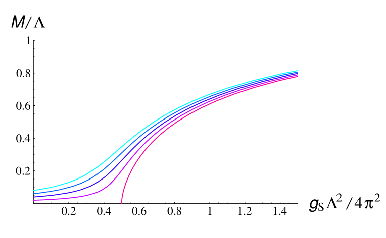
Figure 1: Dynamical quark mass $M/\Lambda$ as a function of the dimensionless coupling constant $g_{\rm S}\Lambda^{2}/4\pi^{2}$ for different current quark masses, $m_{0}/\Lambda=0.08,\,0.06,\,0.04,\,0.02,\,0$ (chiral limit), from top to bottom.

When the coupling constant $g_{\rm S}$ is larger than the critical value $g^{\rm(crit)}_{\rm S}=2\pi^{2}/\Lambda^{2}$, the gap equation (3.13) develops a nonzero solution even in the chiral limit. This is easily confirmed by the numerical solution to the gap equation, as is shown in Fig. 1. Therefore, if we take this nonzero solution and substitute it to the canonical Hamiltonian, we are able to describe the dynamics in the broken phase.

As we will discuss shortly, solving the bilocal fermionic constraints (3.4) and (3.5) up to the next-to-leading order is important for deriving the LC Hamiltonian to the first nontrivial order. In fact, one can even solve the constraints at arbitrarily high order, in the inductive way. Namely, if one knows the solutions up to the $n$-th order, then the $(n+1)$-th order solution is given by some known functions and the solutions whose orders are lower than $n+1$. All the details are discussed in Appendix D, together with the derivation of the LC Hamiltonian.

3.1.2 The LC Hamiltonian

Since the canonical LC Hamiltonian is bilinear with respect to the spinor (see Eq. (D.5)), one can rewrite it by the bilocal operators:

$$H\,=\,P^{-} = \frac{1}{2}\int d^{3}\mbox{\boldmath{$x$}}\int d^{3}\mbox{\boldmath{$y$}}\,\partial^{y}_{j}~{}{\sf V}^{j}_{\rm I}(\mbox{\boldmath{$x$}},\mbox{\boldmath{$y$}})\,\delta(\mbox{\boldmath{$x$}}-\mbox{\boldmath{$y$}})+\frac{m_{0}}{2}\int d^{3}\mbox{\boldmath{$x$}}~{}{\sf S}_{\rm R}(\mbox{\boldmath{$x$}},\mbox{\boldmath{$x$}})$$ (3.14)

$$= \frac{1}{2}\int d^{3}\mbox{\boldmath{$p$}}\int d^{3}\mbox{\boldmath{$q$}}~{}(iq_{\perp}^{j}){\sf V}^{j}_{\rm I}(\mbox{\boldmath{$p$}},\mbox{\boldmath{$q$}})\,\delta(\mbox{\boldmath{$p$}}+\mbox{\boldmath{$q$}})+\frac{m_{0}}{2}\int d^{3}\mbox{\boldmath{$p$}}~{}{\sf S}_{\rm R}(\mbox{\boldmath{$p$}},-\mbox{\boldmath{$p$}})\,,$$

where we have introduced a new bilocal operator,

$$i\,{\sf V}^{j}_{\rm I}(\mbox{\boldmath{$x$}},\mbox{\boldmath{$y$}}) \equiv \bar{\Psi}(\mbox{\boldmath{$x$}})~{}\Lambda_{-}\gamma^{j}_{\perp}\Psi(\mbox{\boldmath{$y$}})-{\rm h.c.}\ \,.$$ (3.15)

Note that this new bilocal operator can be related to the known operators, ${\sf M,\,S,\,P}$ (see Appendix D). Therefore, given the solutions ${\sf s}^{(n)}_{\rm R}$ and ${\sf p}^{(n)}_{\rm R}$, one can immediately obtain ${\sf v}_{\rm I}^{i\,(n)}$, the expansion coefficients of ${\sf V}_{\rm I}^{i}$. Hence, one can compute the LC Hamiltonian order by order

$$H = N\sum_{n=0}^{\infty}\left(\frac{1}{\sqrt{N}}\right)^{n}h^{(n)}_{\rm S}~{},$$ (3.16)

where the subscript S was put in order to remind that this is for the case with ${\cal L}_{\rm S}$ (2.1) (without the vector interaction). We substitute the ”broken” solutions of ${\sf s}^{(n)}_{\rm R}$ and ${\sf p}^{(n)}_{\rm R}$ to obtain the Hamiltonian which describes the broken phase of the chiral symmetry. It turns out that the lowest order $h^{(0)}_{\rm S}$ is divergent but is just a constant, and thus can be neglected for the present purpose. The next order ${\sf v}_{\rm I}^{i~{}(1)}(\mbox{\boldmath{$p$}},{-\mbox{\boldmath{$p$}}})$ and ${\sf s}^{(1)}_{\rm R}(\mbox{\boldmath{$p$}},{-\mbox{\boldmath{$p$}}})$ become strictly zero, and we have $h^{(1)}_{\rm S}=0$. Therefore, the first nontrivial contribution is given by the next-to-leading order $n=2$. After straightforward calculation, one arrives at the following expression (see Appendix D for the derivation):

$$h^{(2)}_{\rm S}\!\! = \!\!\int[d\mbox{\boldmath{$p$}}][d\mbox{\boldmath{$q$}}]~{}\left\{\frac{p_{\perp}^{2}+M^{2}}{2p^{+}}+\frac{q_{\perp}^{2}+M^{2}}{2q^{+}}\right\}\sum_{s_{1},s_{2}}B^{\dagger}(\mbox{\boldmath{$p$}},s_{1}:\mbox{\boldmath{$q$}},s_{2})B(\mbox{\boldmath{$p$}},s_{1}:\mbox{\boldmath{$q$}},s_{2})$$ (3.17)

$$\!\!-\,g_{\rm S}\kappa_{\rm S}\int\frac{[d\mbox{\boldmath{$p$}}][d\mbox{\boldmath{$q$}}][d\mbox{\boldmath{$k$}}][d\mbox{\boldmath{$\l$}}]}{(2\pi)^{3}}\,\frac{\delta(\mbox{\boldmath{$p$}}+\mbox{\boldmath{$q$}}-\mbox{\boldmath{$k$}}-\mbox{\boldmath{$\l$}})}{4\sqrt{p^{+}q^{+}k^{+}l^{+}}}\,\sum_{s_{1},s_{2}}\sum_{s^{\prime}_{1},s^{\prime}_{2}}B^{\dagger}(\mbox{\boldmath{$p$}},s_{1}:\mbox{\boldmath{$q$}},s_{2})B(\mbox{\boldmath{$k$}},s^{\prime}_{1}:\mbox{\boldmath{$\l$}},s^{\prime}_{2})$$

$$\!\!\times\biggl{[}\Big{\{}{\bar{u}}(\mbox{\boldmath{$p$}},s_{1})v(\mbox{\boldmath{$q$}},s_{2})\Big{\}}\,\Big{\{}{\bar{v}}(\mbox{\boldmath{$\l$}},s^{\prime}_{2})u(\mbox{\boldmath{$k$}},s^{\prime}_{1})\Big{\}}+\Big{\{}{\bar{u}}(\mbox{\boldmath{$p$}},s_{1})\,i\gamma_{5}\,v(\mbox{\boldmath{$q$}},s_{2})\Big{\}}\,\Big{\{}{\bar{v}}(\mbox{\boldmath{$\l$}},s^{\prime}_{2})\,i\gamma_{5}\,u(\mbox{\boldmath{$k$}},s^{\prime}_{1})\Big{\}}\biggr{]}\,,\ \ \ \ \ \$$

where we have introduced a constant

$$\kappa_{\rm S}\equiv\left\{1+g_{\rm S}\int\frac{d^{3}\mbox{\boldmath{$r$}}}{(2\pi)^{3}}\frac{\epsilon(r^{+})}{P^{+}-r^{+}}\right\}^{-1}.$$ (3.18)

As already mentioned, in the leading order of the $1/N$ expansion, the bosonic operator $B^{\dagger}(\mbox{\boldmath{$p$}},s_{1}:\mbox{\boldmath{$q$}},s_{2})$ can be interpreted as a creation operator of a quark-antiquark pair (the pair behaves like a boson). Since this Hamiltonian contains only terms of $B^{\dagger}B$ type, it describes the dynamics of the two body $q\bar{q}$ sector. Indeed, the first, diagonal, term corresponds to the free part for this quark-antiquark pair with constituent mass $M$, which is easily understood by the fact that $(p_{\perp}^{2}+M^{2})/2p^{+}+(q_{\perp}^{2}+M^{2})/2q^{+}$ corresponds to the sum of LC energies of a free quark and a free antiquark. The second term, which is proportional to the (scaled) coupling constant and thus clearly comes from the interaction, needs to be diagonalized. As we will see later, diagonalization leads to a bound-state equation for the quark and anti-quark pair.

It is of special importance to recognize that the divergent factor $\kappa_{\rm S}$ defined by Eq. (3.18) is independent of the external momentum $P^{+}$. This is formally seen by changing the variable in the longitudinal integration ($y=r^{+}/P^{+}$)

$$\int_{-\infty}^{\infty}dr^{+}\frac{\epsilon(r^{+})}{P^{+}-r^{+}}=\int_{-\infty}^{\infty}dy\,\frac{\epsilon(y)}{1-y}\,.$$

Of course we need to regularize this integral, but if we use a cutoff which does not depend on the external momentum $P^{+}$, then the result does not depend on $P^{+}$, either. This is true as far as we treat a boost invariant cutoff since the external momentum $P^{+}=p^{+}+q^{+}$ is eventually related to the total momentum of the two body $q\bar{q}$ state (see discussion in the next section).

3.2 The case with vector interaction

Inclusion of the vector interaction certainly complicates the fermionic constraint, but the structure of the constraint (as a differential equation) is the same and we can follow the same procedure as before. Thus, we do not repeat the whole procedure here, but rather present only the differences from the previous case. The main difference is that we have to treat another types of bilocal operators, which makes the number of equations double.

3.2.1 Definition of the bilocal fields

In the case without the vector interaction, the fermionic constraint (2.3) was transformed into two equations (3.4) and (3.5) which form a closed set for bilocal operators ${\sf S}_{\rm R}$ and ${\sf P}_{\rm R}$. On the other hand, when the vector interaction is turned on, the original fermionic constraint (2.4) cannot be expressed only with respect to ${\sf S}_{\rm R}$ and ${\sf P}_{\rm R}$, but we need to introduce another types of operators, the vector ${\sf V}^{\mu}$ and the axial vector ${\sf A}^{\mu}$. Specifically, we define the following bilocal operators:

$${\sf S}(\mbox{\boldmath{$x$}},\mbox{\boldmath{$y$}}) \equiv \bar{\Psi}(\mbox{\boldmath{$x$}})\Lambda_{-}\Psi(\mbox{\boldmath{$y$}})\,,\qquad\qquad{\sf P}(\mbox{\boldmath{$x$}},\mbox{\boldmath{$y$}})\equiv\bar{\Psi}(\mbox{\boldmath{$x$}})\Lambda_{-}(i\gamma_{5})\Psi(\mbox{\boldmath{$y$}}),$$ (3.19)

$${\sf V}^{i}(\mbox{\boldmath{$x$}},\mbox{\boldmath{$y$}}) \equiv \bar{\Psi}(\mbox{\boldmath{$x$}})\Lambda_{-}(\gamma_{\perp}^{i})\Psi(\mbox{\boldmath{$y$}})\,,\quad\quad{\sf V}^{\pm}(\mbox{\boldmath{$x$}},\mbox{\boldmath{$y$}})\equiv\frac{1}{2}\bar{\Psi}(\mbox{\boldmath{$x$}})\gamma^{\pm}\Psi(\mbox{\boldmath{$y$}}),$$ (3.20)

$${\sf A}^{i}(\mbox{\boldmath{$x$}},\mbox{\boldmath{$y$}}) \equiv \bar{\Psi}(\mbox{\boldmath{$x$}})\Lambda_{-}(\gamma_{\perp}^{i}\gamma_{5})\Psi(\mbox{\boldmath{$y$}})\,,\quad{\sf A}^{\pm}(\mbox{\boldmath{$x$}},\mbox{\boldmath{$y$}})\equiv\frac{1}{2}\bar{\Psi}(\mbox{\boldmath{$x$}})\gamma^{\pm}\gamma_{5}\,\Psi(\mbox{\boldmath{$y$}}).$$ (3.21)

For each operator ${\sf O=S,P,V^{\mu},A^{\mu}}$, we further define its ”real” and ”imaginary” parts as follows:

$${\sf O}(\mbox{\boldmath{$x$}},\mbox{\boldmath{$y$}}) = \frac{1}{2}\,\Big{\{}{\sf O}_{\rm R}(\mbox{\boldmath{$x$}},\mbox{\boldmath{$y$}})+i\,{\sf O}_{\rm I}(\mbox{\boldmath{$x$}},\mbox{\boldmath{$y$}})\Big{\}}\,,$$ (3.22)

where

$${\sf O}_{\rm R}(\mbox{\boldmath{$x$}},\mbox{\boldmath{$y$}}) = {\sf O}(\mbox{\boldmath{$x$}},\mbox{\boldmath{$y$}})+{\sf O}(\mbox{\boldmath{$x$}},\mbox{\boldmath{$y$}})^{\dagger},$$

$$i\,{\sf O}_{\rm I}(\mbox{\boldmath{$x$}},\mbox{\boldmath{$y$}}) = {\sf O}(\mbox{\boldmath{$x$}},\mbox{\boldmath{$y$}})-{\sf O}(\mbox{\boldmath{$x$}},\mbox{\boldmath{$y$}})^{\dagger},$$

so that they satisfy ${\sf O}_{\rm R,I}(\mbox{\boldmath{$x$}},\mbox{\boldmath{$y$}})^{\dagger}={\sf O}_{\rm R,I}(\mbox{\boldmath{$x$}},\mbox{\boldmath{$y$}})$. Of course these definitions are consistent with (3.2), (3.3) and (3.15), which were already introduced when we solved the fermionic constraint without vector interaction. Note that all the ”real” parts at the same space-time points (i.e., ${\sf O}_{\rm R}(\mbox{\boldmath{$x$}},\mbox{\boldmath{$x$}})$) reduce to the operators which have appropriate statistics. Namely,

$${\sf S}_{\rm R}(\mbox{\boldmath{$x$}},\mbox{\boldmath{$x$}})=\bar{\Psi}(\mbox{\boldmath{$x$}})\Psi(\mbox{\boldmath{$x$}}),\quad\,\quad\ {\sf P}_{\rm R}(\mbox{\boldmath{$x$}},\mbox{\boldmath{$x$}})=\bar{\Psi}(\mbox{\boldmath{$x$}})\,i\gamma_{5}\,\Psi(\mbox{\boldmath{$x$}}),$$ (3.23)

$${\sf V}_{\rm R}^{\mu}(\mbox{\boldmath{$x$}},\mbox{\boldmath{$x$}})=\bar{\Psi}(\mbox{\boldmath{$x$}})\,\gamma^{\mu}\,\Psi(\mbox{\boldmath{$x$}}),\quad{\sf A}_{\rm R}^{\mu}(\mbox{\boldmath{$x$}},\mbox{\boldmath{$x$}})=\bar{\Psi}(\mbox{\boldmath{$x$}})\,\gamma^{\mu}\gamma_{5}\,\Psi(\mbox{\boldmath{$x$}}).$$ (3.24)

Actually, the operator ${\sf O}(\mbox{\boldmath{$x$}},\mbox{\boldmath{$y$}})$ has been constructed so that ${\sf O}_{\rm R}(\mbox{\boldmath{$x$}},\mbox{\boldmath{$x$}})$ becomes the standard bilinear operator with appropriate statistics. These ”interpolating” operators become useful later when we determine the kinematical structure of the lowest Fock state of a meson.

3.2.2 The bilocal fermionic constraints

Having defined the necessary bilocal operators, we are able to write down a closed set of the bilocal fermionic constraints, which are obviously much involved than the previous case. A closed set is formed by ${\sf S,\,P}$ and the transverse components of vectors ${\sf V}^{i}$ and ${\sf A}^{i}$. Indeed, the explicit form of the bilocal fermionic constraints are given by

$$q^{+}\pmatrix{{\sf S}(\mbox{\boldmath{$p$}},\mbox{\boldmath{$q$}})\cr{\sf P}(\mbox{\boldmath{$p$}},\mbox{\boldmath{$q$}})} = \frac{1}{2}\left\{\pmatrix{1\cr-i\gamma_{5}}\left(\gamma^{j}q_{\perp}^{j}+m_{0}\right)\right\}_{\alpha\beta}{\sf M}_{\alpha\beta}(\mbox{\boldmath{$p$}},\mbox{\boldmath{$q$}})$$ (3.25)

$$-\,\frac{G_{\rm S}}{2}\int\frac{d^{3}\mbox{\boldmath{$k$}}d^{3}\mbox{\boldmath{$\l$}}}{(2\pi)^{3}}\,{\sf M}_{\alpha\beta}(\mbox{\boldmath{$p$}},\mbox{\boldmath{$q$}}-\mbox{\boldmath{$k$}}-\mbox{\boldmath{$\l$}})\,\biggl{\{}\pmatrix{1\cr-i\gamma_{5}}\Big{(}{\sf S}_{\rm R}+i\gamma_{5}~{}{\sf P}_{\rm R}\Big{)}\biggr{\}}_{\alpha\beta}(\mbox{\boldmath{$k$}},\mbox{\boldmath{$\l$}})$$

$$+\,\frac{G_{\rm V}}{2}\int\frac{d^{3}\mbox{\boldmath{$k$}}d^{3}\mbox{\boldmath{$\l$}}}{(2\pi)^{3}}\biggl{[}2\biggl{\{}\Big{(}{\sf S}-i\gamma_{5}\,{\sf P}\Big{)}\pmatrix{1\cr i\gamma_{5}}\biggr{\}}_{\alpha\beta}(\mbox{\boldmath{$p$}},\mbox{\boldmath{$q$}}-\mbox{\boldmath{$k$}}-\mbox{\boldmath{$\l$}}):{\sf M}_{\alpha\beta}(\mbox{\boldmath{$k$}},\mbox{\boldmath{$\l$}}):\biggr{.}$$

$$\hskip 11.38092pt\biggl{.}-\,{\sf M}_{\alpha\beta}(\mbox{\boldmath{$p$}},\mbox{\boldmath{$q$}}-\mbox{\boldmath{$k$}}-\mbox{\boldmath{$\l$}})\,\biggl{\{}\pmatrix{1\cr-i\gamma_{5}}\Big{(}\gamma^{j}:{\sf V}^{j}_{\rm R}:+\gamma^{j}\gamma_{5}\,:{\sf A}^{j}_{\rm R}:\Big{)}\biggr{\}}_{\alpha\beta}(\mbox{\boldmath{$k$}},\mbox{\boldmath{$\l$}})\biggr{]},$$

$$q^{+}\pmatrix{{\sf V}^{i}(\mbox{\boldmath{$p$}},\mbox{\boldmath{$q$}})\cr{\sf A}^{i}(\mbox{\boldmath{$p$}},\mbox{\boldmath{$q$}})} = -\frac{1}{2}\left\{\pmatrix{\gamma^{i}\cr-\gamma^{i}\gamma_{5}}\left(\gamma^{j}q_{\perp}^{j}+m_{0}\right)\right\}_{\alpha\beta}{\sf M}_{\alpha\beta}(\mbox{\boldmath{$p$}},\mbox{\boldmath{$q$}})$$ (3.26)

$$+\,\frac{G_{\rm S}}{2}\int\frac{d^{3}\mbox{\boldmath{$k$}}d^{3}\mbox{\boldmath{$\l$}}}{(2\pi)^{3}}\,{\sf M}_{\alpha\beta}(\mbox{\boldmath{$p$}},\mbox{\boldmath{$q$}}-\mbox{\boldmath{$k$}}-\mbox{\boldmath{$\l$}})\biggl{\{}\pmatrix{\gamma^{i}\cr-\gamma^{i}\gamma_{5}}\Big{(}{\sf S}_{\rm R}+i\gamma_{5}~{}{\sf P}_{\rm R}\Big{)}\biggr{\}}_{\alpha\beta}(\mbox{\boldmath{$k$}},\mbox{\boldmath{$\l$}})$$

$$+\,\frac{G_{\rm V}}{2}\int\frac{d^{3}\mbox{\boldmath{$k$}}d^{3}\mbox{\boldmath{$\l$}}}{(2\pi)^{3}}\biggl{[}2\left\{\left({\sf V}^{i}+\gamma_{5}\,{\sf A}^{i}\right)\pmatrix{1\cr\gamma_{5}}\right\}_{\alpha\beta}(\mbox{\boldmath{$p$}},\mbox{\boldmath{$q$}}-\mbox{\boldmath{$k$}}-\mbox{\boldmath{$\l$}}):{\sf M}_{\alpha\beta}(\mbox{\boldmath{$k$}},\mbox{\boldmath{$\l$}}):\biggr{.}$$

$$\hskip 11.38092pt\biggl{.}+\,{\sf M}_{\alpha\beta}(\mbox{\boldmath{$p$}},\mbox{\boldmath{$q$}}-\mbox{\boldmath{$k$}}-\mbox{\boldmath{$\l$}})\biggl{\{}\pmatrix{\gamma^{i}\cr-\gamma^{i}\gamma_{5}}\left(\gamma^{j}:{\sf V}^{j}_{\rm R}:+\gamma^{j}\gamma_{5}\,:{\sf A}^{j}_{\rm R}:\right)\biggr{\}}_{\alpha\beta}(\mbox{\boldmath{$k$}},\mbox{\boldmath{$\l$}})\biggr{]}\,.\$$

The plus components of the vectors ${\sf V}^{+},\ {\sf A}^{+}$ do not contain the bad spinor and are expressed by ${\sf M}_{\alpha\beta}$, while the minus components ${\sf V}^{-},\ {\sf A}^{-}$ are expressed in terms of ${\sf S,\,P}$, ${\sf V}^{i}$ and ${\sf A}^{i}$. We can solve the above equations following the same procedure as before, though all the calculations are tremendously cumbersome. It should be noticed that the leading order constraint for ${\sf S}$ again leads to the gap equation for the dynamical quark mass $M$, which is equivalent to Eq. (3.13) because we took the normal order in the definition of the vector interaction (2.2).

3.2.3 The LC Hamiltonian

Substituting the solutions of the bilocal fermionic constraints into the canonical LC Hamiltonian, one finds again that the first nontrivial Hamiltonian starts from $n=2$ in the $1/N$ expansion (see, Eq. (3.16)). As a result, the Hamiltonian gets extra terms due to the vector interaction in addition to $h^{(2)}_{\rm S}$ given by (3.17). After a lengthy calculation, one finally obtains (unimportant c-number is ignored)

$$h^{(2)}\!\! = \!\!h^{(2)}_{\rm S}\,+\,\int\frac{[d\mbox{\boldmath{$p$}}][d\mbox{\boldmath{$q$}}][d\mbox{\boldmath{$k$}}][d\mbox{\boldmath{$\l$}}]}{(2\pi)^{3}}\,\,\frac{\delta(\mbox{\boldmath{$p$}}+\mbox{\boldmath{$q$}}-\mbox{\boldmath{$k$}}-\mbox{\boldmath{$\l$}})}{4\sqrt{p^{+}q^{+}k^{+}l^{+}}}$$ (3.27)

$$\hskip 28.45274pt\times\sum_{s_{1},s_{2}}\sum_{s^{\prime}_{1},s^{\prime}_{2}}\Big{(}\omega_{\rm V}+\omega_{\rm SV}+\omega_{\rm V^{2}}+\omega_{\rm SV^{2}}\Big{)}B^{\dagger}(\mbox{\boldmath{$p$}},s_{1}:\mbox{\boldmath{$q$}},s_{2})B(\mbox{\boldmath{$k$}},s^{\prime}_{1}:\mbox{\boldmath{$\l$}},s^{\prime}_{2})\,.$$

The ”kernel” $\omega$’s in the interaction terms are functions of momenta $\mbox{\boldmath{$p$}},\mbox{\boldmath{$q$}},\mbox{\boldmath{$k$}},\mbox{\boldmath{$\l$}}$ and spins $s_{1},s_{2},s_{1}^{\prime},s_{2}^{\prime}$ and given by

$$\omega_{\rm V}\equiv g_{\rm V}\biggl{\{}\kappa_{\rm V}\sum_{\mu=1,2}+\sum_{\mu=+,-}\biggr{\}}\left[\Big{\{}{\bar{u}}(\mbox{\boldmath{$p$}},s_{1})\gamma^{\mu}v(\mbox{\boldmath{$q$}},s_{2})\Big{\}}\Big{\{}{\bar{v}}(\mbox{\boldmath{$\l$}},s^{\prime}_{2})\gamma_{\mu}u(\mbox{\boldmath{$k$}},s^{\prime}_{1})\Big{\}}\right.$$

$$\hskip 170.71652pt\left.+\,\Big{\{}{\bar{u}}(\mbox{\boldmath{$p$}},s_{1})\gamma^{\mu}\gamma_{5}v(\mbox{\boldmath{$q$}},s_{2})\Big{\}}\Big{\{}{\bar{v}}(\mbox{\boldmath{$\l$}},s^{\prime}_{2})\gamma_{\mu}\gamma_{5}u(\mbox{\boldmath{$k$}},s^{\prime}_{1})\Big{\}}\right]\,,$$ (3.28)

$$\omega_{\rm SV}\equiv ig_{\rm S}g_{\rm V}\kappa_{\rm S}\int\frac{d\mbox{\boldmath{$b$}}d\mbox{\boldmath{$c$}}}{(2\pi)^{3}}\,\frac{\epsilon(b^{+})M}{b^{+}c^{+}}\,$$

$$\quad\times\left[\delta(\mbox{\boldmath{$p$}}+\mbox{\boldmath{$q$}}+\mbox{\boldmath{$b$}}+\mbox{\boldmath{$c$}})\,\Big{\{}{\bar{u}}(\mbox{\boldmath{$p$}},s_{1})\gamma^{+}\gamma_{5}v(\mbox{\boldmath{$q$}},s_{2})\Big{\}}\Big{\{}{\bar{v}}(\mbox{\boldmath{$\l$}},s^{\prime}_{2})i\gamma_{5}u(\mbox{\boldmath{$k$}},s^{\prime}_{1})\Big{\}}\right.$$

$$\hskip 96.73918pt\left.+\delta(\mbox{\boldmath{$k$}}+\mbox{\boldmath{$\l$}}-\mbox{\boldmath{$b$}}-\mbox{\boldmath{$c$}})\,\Big{\{}{\bar{u}}(\mbox{\boldmath{$p$}},s_{1})i\gamma_{5}v(\mbox{\boldmath{$q$}},s_{2})\Big{\}}\Big{\{}{\bar{v}}(\mbox{\boldmath{$\l$}},s^{\prime}_{2})\gamma^{+}\gamma_{5}u(\mbox{\boldmath{$k$}},s^{\prime}_{1})\Big{\}}\right]\,,$$ (3.29)

$$\omega_{\rm V^{2}}\equiv g_{\rm V}^{2}\int\frac{d\mbox{\boldmath{$b$}}d\mbox{\boldmath{$c$}}}{(2\pi)^{3}}\,\frac{\epsilon(b^{+})(b^{2}_{\perp}+M^{2})}{b^{+}b^{+}c^{+}}\,\delta(\mbox{\boldmath{$p$}}+\mbox{\boldmath{$q$}}-\mbox{\boldmath{$b$}}-\mbox{\boldmath{$c$}})$$ (3.30)

$$\quad\times\left[\Big{\{}{\bar{u}}(\mbox{\boldmath{$p$}},s_{1})\gamma^{+}v(\mbox{\boldmath{$q$}},s_{2})\Big{\}}\Big{\{}{\bar{v}}(\mbox{\boldmath{$\l$}},s^{\prime}_{2})\gamma^{+}u(\mbox{\boldmath{$k$}},s^{\prime}_{1})\Big{\}}+\Big{\{}{\bar{u}}(\mbox{\boldmath{$p$}},s_{1})\gamma^{+}\gamma_{5}v(\mbox{\boldmath{$q$}},s_{2})\Big{\}}\Big{\{}{\bar{v}}(\mbox{\boldmath{$\l$}},s^{\prime}_{2})\gamma^{+}\gamma_{5}u(\mbox{\boldmath{$k$}},s^{\prime}_{1})\Big{\}}\right]\,,$$

$$\omega_{\rm SV^{2}}\equiv g_{\rm S}g_{\rm V}^{2}\kappa_{\rm S}\int\frac{d\mbox{\boldmath{$b$}}d\mbox{\boldmath{$c$}}d\mbox{\boldmath{$b$}}^{\prime}d\mbox{\boldmath{$c$}}^{\prime}}{(2\pi)^{3}}\,\frac{\epsilon(b^{+})M}{b^{+}c^{+}}\frac{\epsilon(b^{\prime+})M}{b^{\prime+}c^{\prime+}}\,$$ (3.31)

$$\hskip 56.9055pt\times\delta(\mbox{\boldmath{$p$}}+\mbox{\boldmath{$q$}}+\mbox{\boldmath{$b$}}+\mbox{\boldmath{$c$}})\,\delta(\mbox{\boldmath{$k$}}+\mbox{\boldmath{$\l$}}-\mbox{\boldmath{$b$}}^{\prime}-\mbox{\boldmath{$c$}}^{\prime})\Big{\{}{\bar{u}}(\mbox{\boldmath{$p$}},s_{1})\gamma^{+}\gamma_{5}v(\mbox{\boldmath{$q$}},s_{2})\Big{\}}\Big{\{}{\bar{v}}(\mbox{\boldmath{$\l$}},s^{\prime}_{2})\gamma^{+}\gamma_{5}u(\mbox{\boldmath{$k$}},s^{\prime}_{1})\Big{\}}\,,$$

where we have introduced another type of divergent constant

$$\kappa_{\rm V}=\left\{1+g_{\rm V}\int\frac{d^{3}\mbox{\boldmath{$r$}}}{(2\pi)^{3}}\frac{\epsilon(r^{+})}{P^{+}-r^{+}}\right\}^{-1}\,.$$ (3.32)

Notice that $\kappa_{\rm V}$ is independent of the external momentum $P^{+}$ due to exactly the same reason as for $\kappa_{\rm S}$ given by Eq. (3.18).

A few comments are in order about this LC Hamiltonian. First of all, we have introduced the rescaled vector coupling constant $g_{\rm V}=G_{\rm V}N$ which naturally yields the $1/N$ expansion of the LC Hamiltonian. Otherwise all the interaction terms become larger than $h_{\rm S}^{(2)}$ in the $1/N$ counting, which is not interesting. Next, it is clear that all the interaction terms are of the $B^{\dagger}B$ type. This means that the Hamiltonian does not mix the Fock components with different number of particles. Namely, we can solve the Hamiltonian within a small Fock space with one boson (or, equivalently, a $q\bar{q}$ pair).

Lastly, it would be necessary to explain why we obtained terms like $\omega_{\rm SV}$ and $\omega_{\rm SV^{2}}$ which are of the higher order with respect to $G_{\rm S}$ and $G_{\rm V}$, which seems less trivial compared to the case without the vector interaction. The mathematical reasons are the following: First, the bilocal fermionic constraints (3.25) and (3.26) have contributions proportional to $G_{\rm S}$ or $G_{\rm V}$. Thus, it is natural that the solutions to the fermionic constraints, in each order of the $1/N$ expansion, can depend upon $G_{\rm S}$ or $G_{\rm V}$. On the other hand, the LC Hamiltonian contains ${\sf V}^{i}_{\rm I}$, and this vector is again represented by other bilocal operators. Therefore, if we substitute the solutions (which depends on $G_{\rm S}$ and $G_{\rm V}$) to ${\sf V}^{i}_{\rm I}$ in the LC Hamiltonian, there appear higher-order terms with respect to $G_{\rm S}$ or $G_{\rm V}$.

4 Bound-state equations of light mesons

4.1 Interpolating fields and the lowest Fock state representation of mesons

In the leading order of the $1/N$ expansion, mesonic states are expressed as ”constituent” states with a dynamical quark-antiquark pair, as was discussed in Ref. [4]. For the purpose of constructing a meson with appropriate statistics, the first thing to do is to determine its kinematical structure. This can be done in such a way that the mesonic state has the same structure as that of its interpolating field. Namely, a part of the LC wavefunction which rather trivially depends on the statistics can be determined even without solving the dynamical bound-state equation. Then, after extracting this known part, we can define the spin-independent part of the LC wavefunctions.

As we already discussed, the interpolating fields are given by the ”real” parts of the bilocal operators at the same space-time points (see Eqs. (3.23), (3.24)). We can find their explicit forms in terms of spinors and the bilocal boson operators, by using the solutions to the bilocal fermionic constraints. Since (in this subsection) we are interested in the kinematical structures which is independent of the dynamics, we are allowed to use the solutions to the fermionic constraint without the vector interaction. To the leading order, one finds for the scalar and pseudo-scalar fields

$$\pmatrix{\bar{\Psi}(\mbox{\boldmath{$x$}})\Psi(\mbox{\boldmath{$x$}})\cr\bar{\Psi}(\mbox{\boldmath{$x$}})i\gamma_{5}\Psi(\mbox{\boldmath{$x$}})} = \pmatrix{{\sf S}_{\rm R}(\mbox{\boldmath{$x$}},\mbox{\boldmath{$x$}})\cr{\sf P}_{\rm R}(\mbox{\boldmath{$x$}},\mbox{\boldmath{$x$}})}$$

$$= ~{}\sqrt{N}\int\frac{[d\mbox{\boldmath{$P$}}]}{(2\pi)^{3}}\left[\ {\rm e}^{-i\mbox{\boldmath{$P$}}\mbox{\boldmath{$x$}}}~{}\int_{0}^{P^{+}}dk^{+}\int d^{2}k_{\perp}\frac{\kappa_{\rm S}}{2\sqrt{k^{+}(P-k)^{+}}}\right.$$

$$\left.\times\sum_{s_{1},s_{2}}\Big{\{}{\bar{u}}(\mbox{\boldmath{$k$}},s_{1})\pmatrix{1\cr i\gamma_{5}}v(\mbox{\boldmath{$P$}}-\mbox{\boldmath{$k$}},s_{2})\Big{\}}B^{{\dagger}}(\mbox{\boldmath{$k$}},s_{1}:\mbox{\boldmath{$P$}}-\mbox{\boldmath{$k$}},s_{2})\ +{\rm h.c.}\ \right]+{\cal O}(N^{0})\,,$$

and for the vector

$$\bar{\Psi}(\mbox{\boldmath{$x$}})\gamma^{\mu}\Psi(\mbox{\boldmath{$x$}}) = {\sf V}^{\mu}_{\rm R}(\mbox{\boldmath{$x$}},\mbox{\boldmath{$x$}})$$

$$= ~{}\sqrt{N}\int\frac{[d\mbox{\boldmath{$P$}}]}{(2\pi)^{3}}\left[\,{\rm e}^{-i\mbox{\boldmath{$P$}}\mbox{\boldmath{$x$}}}~{}\int_{0}^{P^{+}}dk^{+}\int d^{2}k_{\perp}\frac{1}{2\sqrt{k^{+}(P-k)^{+}}}\right.$$

$$\left.\times\sum_{s_{1},s_{2}}\Big{\{}{\bar{u}}(\mbox{\boldmath{$k$}},s_{1})\gamma^{\mu}v(\mbox{\boldmath{$P$}}-\mbox{\boldmath{$k$}},s_{2})\Big{\}}B^{{\dagger}}(\mbox{\boldmath{$k$}},s_{1}:\mbox{\boldmath{$P$}}-\mbox{\boldmath{$k$}},s_{2})+{\rm h.c.}\right]+{\cal O}(N^{0})\,.$$

The four interpolating fields of the vector are obtained separately for the LC components $\mu=\pm$ and the transverse components $\mu=1,2$, but it turns out that they can be combined to give the reasonable representation as above. The mismatch in the expressions above between $({\sf S,P})$ and ${\sf V}$ (namely, a factor $\kappa_{\rm S}$ in Eq. (4.1)) is due to our use of the solutions with ${\cal L}_{\rm S}\neq 0$ and ${\cal L}_{\rm V}=0$, and would be absent if one used the free field solutions. Needless to say, this difference is irrelevant for the present purpose of determining the kinematical structure.

Since the interpolating fields are all defined at a single spatial point, they can be interpreted as a kind of point-like states without spatial structure. However, what we are interested in is the spatial structure of mesons, and it is indeed the (spin-independent part of the) LC wavefunction which is responsible for this spatial structure. (In other words, for the interpolating fields without spatial structure, the LC wavefunctions are simply constant in momentum space.) First of all, the mesonic states having total momentum $P$ can be represented as follows ($x=k^{+}/P^{+}$):

$$\left.\left|\,{\rm meson}\,;\mbox{\boldmath{$P$}}\,\right.\right\rangle=P^{+}\int_{0}^{1}{dx}\int d^{2}k_{\perp}~{}\sum_{s_{1},s_{2}}\Phi_{\rm meson}(x,k_{\perp},s_{1},s_{2})B^{\dagger}(\mbox{\boldmath{$k$}},s_{1}:\mbox{\boldmath{$P$}}-\mbox{\boldmath{$k$}},s_{2})\left.\left|0\right.\right\rangle\,,$$ (4.3)

where $\Phi_{\rm meson}(x,\mbox{\boldmath{$k$}}_{\perp},s_{1},s_{2})$ is the LC wavefunction of the $q\bar{q}$ Fock state, and the vacuum is defined by the bilocal boson operator

$$B(\mbox{\boldmath{$p$}},s_{1}:\mbox{\boldmath{$q$}},s_{2})\left.\left|0\right.\right\rangle=0\,.$$ (4.4)

Notice that this vacuum is equivalent to the one defined by the quark antiquark operators to the leading order of the $1/N$ expansion. From the interpolating fields shown above, we can determine the kinematical structure (or, spin-dependent parts) of the LC wavefunctions:

$$\Phi_{\pi}(x,k_{\perp},s_{1},s_{2}) \equiv \frac{1}{2\sqrt{x(1-x)}}\,\phi_{\pi}(x,k_{\perp})\,\Big{\{}{\bar{u}}(\mbox{\boldmath{$k$}},s_{1})\,i\gamma_{5}\,v({\mbox{\boldmath{$P$}}}-\mbox{\boldmath{$k$}},s_{2})\Big{\}},$$ (4.5)

$$\Phi_{\sigma}(x,k_{\perp},s_{1},s_{2}) \equiv \frac{1}{2\sqrt{x(1-x)}}\,\phi_{\sigma}(x,k_{\perp})\,\Big{\{}{\bar{u}}(\mbox{\boldmath{$k$}},s_{1})\,v({\mbox{\boldmath{$P$}}}-\mbox{\boldmath{$k$}},s_{2})\Big{\}},$$ (4.6)

$$\Phi_{\rho}^{\lambda}(x,k_{\perp},s_{1},s_{2}) \equiv \frac{1}{2\sqrt{x(1-x)}}\,\phi_{\rho}(x,k_{\perp})\,\epsilon_{\mu}(\lambda,P)\Big{\{}{\bar{u}}(\mbox{\boldmath{$k$}},s_{1})\,\gamma^{\mu}\,v({\mbox{\boldmath{$P$}}}-\mbox{\boldmath{$k$}},s_{2})\Big{\}}\,,$$ (4.7)

where we have introduced the spin-independent LC wavefunction $\phi(x,k_{\perp})$ for each meson. These expressions are valid when $P_{\perp}=0$ . The corresponding formulae for $P_{\perp}\neq 0$ are shown in Appendix E. For the vector meson, we have already introduced 3 physical states $\left.\left|\rho,\lambda\right.\right\rangle$ with helicity $\lambda=\pm 1,0$ (see Eq. (4.7)) which should be distinguished from 4 states $\left.\left|\rho^{\mu}\right.\right\rangle$ naively constructed from the interpolating field without the polarization vector $\epsilon_{\mu}(\lambda,P)$. Below, we will explain the necessity of using $\left.\left|\rho,\lambda\right.\right\rangle$ instead of $\left.\left|\rho^{\mu}\right.\right\rangle$.

One can directly verify the orthogonality among these mesonic states. For example, let us check the orthogonality between the scalar $\left.\left|\sigma\right.\right\rangle$ and the vector $\left.\left|\rho^{\mu}\right.\right\rangle$ when the transverse momentum of the meson $P_{\perp}$ is zero:

$$\left\langle\left.\,\sigma;P^{+},P_{\perp}=0\,\right|\right.\,\rho^{\mu};P^{\prime+},P^{\prime}_{\perp}=0\,\rangle$$ (4.8)

$$= \delta(\mbox{\boldmath{$P$}}-\mbox{\boldmath{$P$}}^{\prime})|_{P_{\perp}=0}\,P^{+}\int_{0}^{1}\frac{dx}{4x(1-x)}\int_{-\infty}^{\infty}d^{2}k_{\perp}{\phi}^{*}_{\sigma}(x,k_{\perp}){\phi}_{\rho}(x,k_{\perp})$$

$$\hskip 28.45274pt\times\sum_{s_{1},s_{2}}~{}\Big{\{}{\bar{u}}(\mbox{\boldmath{$k$}},s_{1})\,\gamma^{\mu}\,v(\mbox{\boldmath{$P$}}-\mbox{\boldmath{$k$}},s_{2})\Big{\}}\Big{\{}{\bar{v}}(\mbox{\boldmath{$P$}}-\mbox{\boldmath{$k$}},s_{2})\,u(\mbox{\boldmath{$k$}},s_{1})\Big{\}}\Big{|}_{P_{\perp}=0}\,,$$

where the quantity on the last line can be evaluated as

$$\sum_{s_{1},s_{2}}~{}\Big{\{}{\bar{u}}(\mbox{\boldmath{$k$}},s_{1})\,\gamma^{\mu}\,v(\mbox{\boldmath{$P$}}-\mbox{\boldmath{$k$}},s_{2})\Big{\}}\Big{\{}{\bar{v}}(\mbox{\boldmath{$P$}}-\mbox{\boldmath{$k$}},s_{2})\,u(\mbox{\boldmath{$k$}},s_{1})\Big{\}}\Big{|}_{P_{\perp}=0}$$ (4.12)

$$= \left\{\begin{array}[]{ll}-8Mk^{i}_{\perp}\,,&\;\mbox{ $\mu=i=1,2$ }\\ 4MP^{+}(1-2x)\,,&\;\mbox{ $\mu=+$ }\\ -\frac{4M}{2P^{+}}\frac{(1-2x)}{x(1-x)}\,(k^{2}_{\perp}+M^{2})\,,&\;\mbox{ $\mu=-$ }.\end{array}\right.$$

Assuming that the spin-independent wavefunctions are functions of $x(1-x)$ and $k_{\perp}^{2}$ (which can be checked a posteriori, but is natural due to the charge symmetry), one concludes that the bracket $\left\langle\left.\sigma\right|\right.\rho^{\mu}\rangle$ above is zero for all $\mu$. The orthogonality for other combinations of the states are verified too in a similar way.

It should be noticed that the four vector states $\left.\left|\rho^{\mu}\right.\right\rangle$ are not independent of each other (thus not necessarily orthogonal to each other), since a real massive vector meson should have only three physical modes, i.e., two transverse and one longitudinal modes. This can be seen by the fact that the spinor part of the state (4.7) satisfies the following identity:

$$(E_{k}+E_{(P-k)})\left[{\bar{u}}(\mbox{\boldmath{$k$}},s_{1})\gamma^{+}\,v(\mbox{\boldmath{$P$}}-\mbox{\boldmath{$k$}},s_{2})\right]+P^{+}\left[{\bar{u}}(\mbox{\boldmath{$k$}},s_{1})\gamma^{-}\,v(\mbox{\boldmath{$P$}}-\mbox{\boldmath{$k$}},s_{2})\right]$$

$$-P_{\perp}^{i}\left[{\bar{u}}(\mbox{\boldmath{$k$}},s_{1})\gamma^{i}\,v(\mbox{\boldmath{$P$}}-\mbox{\boldmath{$k$}},s_{2})\right]=0$$

where $E_{k}$ and $E_{P-k}$ are the LC energies of the quark and the antiquark

$$E_{k}\equiv\frac{k_{\perp}^{2}+M^{2}}{2k^{+}},\qquad E_{(P-k)}\equiv\frac{(P-k)_{\perp}^{2}+M^{2}}{2(P-k)^{+}}\,.$$ (4.13)

The projection onto three physical modes can be easily done by the circular polarization vector $\epsilon^{\mu}(\lambda,P)$. As we already introduced in Eq. (4.7), three independent states with helicity $\lambda=\pm 1,0$ are given by

$$\left.\left|\,\rho,\lambda\,;\mbox{\boldmath{$P$}}\,\right.\right\rangle\equiv\epsilon_{\mu}(\lambda,P)\left.\left|\,\rho^{\mu}\,;\mbox{\boldmath{$P$}}\,\right.\right\rangle.$$ (4.14)

These three states are orthogonal: $\left\langle\left.\,\rho,\lambda\,\right|\right.\,\rho,\lambda^{\prime}\,\rangle=0$ for $\lambda\neq\lambda^{\prime}$. In the frame where the transverse momentum of the vector meson is zero, $\mbox{\boldmath{$P$}}=(P^{+},P_{\perp})=(P^{+},0_{\perp})$, the polarization vectors are given by ($\epsilon^{\mu}=(\epsilon^{+},\epsilon^{-},\epsilon^{1},\epsilon^{2})$ ) [13]

$$\epsilon^{\mu}(\lambda=\pm 1,P) = (0,0,\mp\frac{1}{\sqrt{2}},-\frac{i}{\sqrt{2}})\,,$$ (4.15)

$$\epsilon^{\mu}(\lambda=0,P) = (\frac{P^{+}}{m_{\rm V}},-\frac{m_{\rm V}}{2P^{+}},0,0)\,,$$ (4.16)

satisfying $\epsilon_{\mu}(\lambda,P)\epsilon^{\mu}(\lambda^{\prime},P)^{*}=-\delta_{\lambda\lambda^{\prime}},~{}P_{\mu}\epsilon^{\mu}(\lambda,P)=0$. Therefore, the explicit relations between $\left.\left|\rho^{\mu}\right.\right\rangle$ and the physical states $\left.\left|\rho,\lambda\right.\right\rangle$ are

$$\left.\left|\,\rho,\lambda=\pm 1\,\right.\right\rangle=\pm\frac{1}{\sqrt{2}}\,|\,\rho^{1}\,\rangle+\frac{i}{\sqrt{2}}\,|\,\rho^{2}\,\rangle\,,$$ (4.17)

$$\left.\left|\,\rho,\lambda=0\,\right.\right\rangle=\frac{-m_{\rm V}}{2P^{+}}\,|\,\rho^{+}\,\rangle+\frac{P^{+}}{m_{\rm V}}\,|\,\rho^{-}\,\rangle\,.$$ (4.18)

Notice that these relations are valid only in the frame $\mbox{\boldmath{$P$}}=(P^{+},0_{\perp})$, and does not hold any longer if one moves to other reference frame.

In summary, the orthogonality holds among the five mesonic states: $\left.\left|\sigma\right.\right\rangle,\,\left.\left|\pi\right.\right\rangle$ and $\left.\left|\rho,\lambda\right.\right\rangle$ with $\lambda=\pm 1,0$. Therefore, together with the normalization of each state, we obtain

$$\langle\alpha,\mbox{\boldmath{$P$}}\left.\left|\alpha^{\prime},\mbox{\boldmath{$P$}}^{\prime}\right.\right\rangle=16\pi^{3}P^{+}\,\delta_{\alpha,\alpha^{\prime}}\,\delta({\mbox{\boldmath{$P$}}}-{\mbox{\boldmath{$P$}}^{\prime}}),$$ (4.19)

where $\alpha$ ($\alpha^{\prime}$) distinguishes the species of meson $\alpha=\sigma,\pi,\,(\rho,\lambda)$. This also leads to the normalization condition for the LC wavefunctions:

$$\frac{1}{16\pi^{3}}\int_{0}^{1}dx\,\int_{-\infty}^{\infty}d^{2}k_{\perp}~{}\sum_{s_{1},s_{2}}|\Phi_{\alpha}(x,k_{\perp},s_{1},s_{2})|^{2}=1.$$ (4.20)

4.2 Bound-state equations

Before going into details, let us briefly discuss a generic $q\bar{q}$ state in order to clarify the procedure we perform. In general, the LF energy of the two body state may be schematically written as

$$P^{-}_{q\bar{q}}=\frac{k_{\perp}^{2}+M^{2}}{2k^{+}}+\frac{(P_{\perp}-k_{\perp})^{2}+M^{2}}{2(P^{+}-k^{+})}+V(k,P),$$ (4.21)

where the first two terms are the ”kinetic” energies of the quark and the antiquark, and $V$ is the potential which allows for a bound state. This form of the energy leads to the following bound-state equation:

$$\left\{m_{\rm meson}^{2}-\frac{k_{\perp}^{2}+M^{2}}{x(1-x)}\right\}\phi(x,k_{\perp})=\int_{0}^{1}dy\int d^{2}p_{\perp}\,V(x,k_{\perp};y,p_{\perp})\,\phi(y,p_{\perp})\,,$$ (4.22)

where we have chosen $\mbox{\boldmath{$P$}}=(P^{+},P_{\perp}^{i})=(P^{+},\,0_{\perp})$ for simplicity, and redefined $V$ with some factors included.

For the scalar and pseudo-scalar mesons, the potential $V$ has a simple structure, and we can evaluate it without any further approximation. On the other hand, for the vector mesons, $V$ has nontrivial dependencies upon $g_{\rm V}$. For the present purpose of seeing the leading effects of the vector interaction (2.2) on the vector channel, it is actually enough to derive the potential $V$ up to the leading order of the vector interaction $g_{\rm V}$. We will see that in this leading order the potential term $V(x,k_{\perp};y,p_{\perp})$ is separable with respect to the internal $(y,p_{\perp})$ and external $(x,k_{\perp})$ variables, and actually depends only on $y$ and $p_{\perp}$.

In the following, we are going to derive a bound-state equation for each meson in the frame $\mbox{\boldmath{$P$}}=(P^{+},\,0_{\perp})$, which is simply deduced from the light-front eigen-value equation:

$$P^{-}\left.\left|\,{\rm meson}\,;P^{+},P_{\perp}=0\right.\right\rangle~{}=\frac{m_{\rm meson}^{2}}{2P^{+}}\left.\left|\,{\rm meson}\,;P^{+},P_{\perp}=0\right.\right\rangle\,.$$ (4.23)

To the first non-trivial order in the $1/N$ expansion, this equation can be restricted to the $q\bar{q}$ subspace of the Fock space, leading to the bound-state equation for mesons.

4.2.1 Scalar and pseudo-scalar mesons

It is straightforward to derive the bound-state equations for scalar and pseudo-scalar mesons. In Eq. (4.23), we use the LC Hamiltonian $P^{-}=h^{(2)}_{\rm S}$ defined in Eq. (3.17) (recall our strategy for scalar and pseudo-scalar mesons, see Sect. 2.1) and the scalar and pseudo-scalar states given by Eqs. (4.6), (4.5). Then, one obtains

$$\left\{m_{\sigma}^{2}-\frac{k_{\perp}^{2}+M^{2}}{x(1-x)}\right\}\phi_{\sigma}(x,k_{\perp})=-\frac{g_{\rm S}\kappa_{\rm S}}{(2\pi)^{3}}\int_{0}^{1}dy\int d^{2}p_{\perp}\frac{p_{\perp}^{2}+(1-2y)^{2}M^{2}}{y^{2}(1-y)^{2}}\phi_{\sigma}(y,p_{\perp})\,,$$ (4.24)

$$\left\{m_{\pi}^{2}-\frac{k_{\perp}^{2}+M^{2}}{x(1-x)}\right\}\phi_{\pi}(x,k_{\perp})=-\frac{g_{\rm S}\kappa_{\rm S}}{(2\pi)^{3}}\int_{0}^{1}dy\int d^{2}p_{\perp}\frac{p_{\perp}^{2}+M^{2}}{y^{2}(1-y)^{2}}\phi_{\pi}(y,p_{\perp})\,.$$ (4.25)

An important property to be noticed is the fact that, in both cases, the potential terms (the right-hand sides) are independent of the external variables $x,\ k_{\perp}$. This property is due to the simple structure of the contact interaction ${\cal L}_{\rm S}$. The same thing will be seen in the case of the vector meson. These results are equivalent to the previous ones obtained in Ref. [4]. Formal solutions to these equations are easily obtained (due to the simple structure of the potential terms), but we postpone to discuss them until the next section, where we present the LC wavefunctions and masses of the mesons after careful evaluation of divergences.

4.2.2 Vector mesons

For a vector meson, the first nontrivial contribution (in the $1/N$ expansion) of the LC Hamiltonian is given by $P^{-}=h^{(2)}$ in Eq. (3.27), and the transverse and longitudinal states are given by Eqs. (4.17) and (4.18), respectively. Although the mass and the spin-independent LC wavefunction must be, by definition, the same for both the transverse and longitudinal polarizations, we distinguish the bound-state equations for these two modes since they appear differently until we perform careful regularization of the divergences. Therefore, in the following, we use notations like $V_{\rm T/L},\ \phi_{\rm T/L}(x,k_{\perp}),$ and $m_{\rm T/L}$ for corresponding transverse and longitudinal quantities (though eventually they are proven to be equivalent to each other).

For a transversely polarized vector meson, a lengthy calculation yields the following potential $V_{\rm T}$ (in the sense of Eq. (4.22))

$$V_{\rm T}=-\,\,\frac{g_{\rm V}}{(2\pi)^{3}}\left[1+\frac{g_{\rm V}}{(2\pi)^{3}}\int_{-\infty}^{\infty}dq^{+}\int d^{2}q_{\perp}\frac{\epsilon(q^{+})}{P^{+}-q^{+}}\right]^{-1}\frac{p_{\perp}^{2}+M^{2}-2y(1-y)p_{\perp}^{2}}{y^{2}(1-y)^{2}}\,.$$ (4.26)

This potential comes from $\omega_{\rm V}$ in the LC Hamiltonian (3.27). The other terms do not contribute to the bound-state equation because of the orthogonality among the bispinors. Notice that the potential is already independent of the external variables $x,k_{\perp}$. Taking the leading contribution of $g_{\rm V}$, one arrives at an equation for the LC wavefunction $\phi_{\rm T}(x,k_{\perp})=\phi_{\lambda=\pm 1}(x,k_{\perp})$:

$$\left\{m_{\rm T}^{2}-\frac{k_{\perp}^{2}+M^{2}}{x(1-x)}\right\}\phi_{\rm T}(x,k_{\perp})=-\,\frac{g_{\rm V}}{(2\pi)^{3}}\int_{0}^{1}dy\int d^{2}p_{\perp}\frac{p_{\perp}^{2}+M^{2}-2y(1-y)p_{\perp}^{2}}{y^{2}(1-y)^{2}}\,\phi_{\rm T}(y,p_{\perp}).$$ (4.27)

Since we pick up the leading contribution in Eq. (4.26), the divergent factor in the square bracket is now replaced by 1. This factor is the explicit expression of $\kappa_{\rm V}$ which appeared in the Hamiltonian (cf: see Eq. (3.32)), and if we keep this factor, the structure of the bound-state equation looks similar to those of the scalar and pseudo-scalar mesons (their potential terms are proportional to $g_{\rm S}\kappa_{\rm S}$). However, as we will see below, the corresponding equation for the longitudinal mode does not have the same simple structure, and we keep the leading order effect (namely, $\kappa_{\rm V}=1$) for simplicity.

The longitudinally polarized state is much more involved. One of the main complexity comes from the fact that ${\sf V}^{+}$ and ${\sf V}^{-}$ are treated (and in fact do behave) differently in the light-front quantization, while the physical longitudinal mode is a linear combination between these two. This situation requires a longer and attentive, but still straightforward, calculation which eventually leads to the following potential $V_{\rm L}$ (for the details of the derivation, see Appendix F):

$$V_{\rm L} \!\!= \!\!-\frac{g_{\rm V}}{(2\pi)^{3}}\left\{1-2\frac{g_{\rm V}}{(2\pi)^{3}}\int_{0}^{1}dz\int d^{2}q_{\perp}\right\}^{-1}\left\{m_{\rm L}^{2}-\frac{k_{\perp}^{2}+M^{2}}{x(1-x)}\right\}\left\{m_{\rm L}^{2}+\frac{k_{\perp}^{2}+M^{2}}{x(1-x)}\right\}^{-1}$$ (4.28)

$$\times \left[\,2\,+\,\frac{4\,(k_{\perp}^{2}+M^{2})}{m_{\rm L}^{2}\,x(1-x)-(k_{\perp}^{2}+M^{2})}\left\{1-\frac{g_{\rm V}}{(2\pi)^{3}}\int_{0}^{1}\!dz\!\int\!d^{2}q_{\perp}\right\}\right]\left\{m_{\rm L}^{2}\,+\frac{p_{\perp}^{2}+M^{2}}{y(1-y)}\,\right\}.$$

It should be noticed that the interaction term $\omega_{\rm V^{2}}$ in the LC Hamiltonian (3.27) as well as $\omega_{\rm V}$ contributes to the longitudinal potential while it does not contribute to the transverse potential. As we mentioned above, the $g_{\rm V}$ dependence is not the same as the transverse case, and is much more non-trivial. However, we obtain a simpler result by taking the ”leading term” with respect to $g_{\rm V}$ in this potential (more precisely, in the eigen-value equation). Here we give a quick, but less systematic, derivation of the final result. (A more detailed derivation is explained in Appendix F.) This can be done as follows: First of all, we ignore the $g_{\rm V}$ dependent term in the second line of Eq. (4.28) that gives the higher order in $g_{\rm V}$ and thus can be ignored anyway. We immediately find

$$\left\{m_{\rm L}^{2}-\frac{k_{\perp}^{2}+M^{2}}{x(1-x)}\right\}\left\{m_{\rm L}^{2}+\frac{k_{\perp}^{2}+M^{2}}{x(1-x)}\right\}^{-1}\left[\,2\,+\,\frac{4\,(k_{\perp}^{2}+M^{2})}{m_{\rm L}^{2}\,x(1-x)-(k_{\perp}^{2}+M^{2})}\right]=2\,.$$

Then we integrate the resulting bound-state equation over $x$ and $k_{\perp}$, obtaining the following:

$$\int dx\,d^{2}k_{\perp}\left\{m_{\rm L}^{2}-\frac{k_{\perp}^{2}+M^{2}}{x(1-x)}\right\}\phi_{\rm L}(x,k_{\perp})=-4\frac{g_{\rm V}}{(2\pi)^{3}}\left(\int dx\,d^{2}k_{\perp}\right)\int dy\,d^{2}p_{\perp}\frac{p_{\perp}^{2}+M^{2}}{y(1-y)}\,\phi_{\rm L}(y,p_{\perp}).$$

Here we have kept the $g_{\rm V}$ dependent term in the curly bracket in the first line of Eq. (4.28). We can modify the bound-state equation by using this relation in the right-hand side of it. Taking the leading term with respect to $g_{\rm V}$, we finally obtain the following simpler equation for the longitudinal mode $\phi_{\rm L}(x,k_{\perp})=\phi_{\lambda=0}(x,k_{\perp})$:

$$\left\{m_{\rm L}^{2}-\frac{k_{\perp}^{2}+M^{2}}{x(1-x)}\right\}\phi_{\rm L}(x,k_{\perp})=-\,\frac{g_{\rm V}}{(2\pi)^{3}}\int_{0}^{1}dy\int d^{2}p_{\perp}\frac{4(p_{\perp}^{2}+M^{2})}{y(1-y)}\,\phi_{\rm L}(y,p_{\perp})\,.$$ (4.29)

It is evident that the right-hand side is again independent of the variables $x,k_{\perp}$. The derivation of Eq. (4.29) looks tricky, but we can obtain the same result by carefully taking the leading order effect with respect to $g_{\rm V}$ in the eigen-value equation (see Appendix F).

Now we obtained the bound-state equations for the transverse and longitudinal modes (i.e., Eqs. (4.27) and (4.29) ). However, at first glance, these two look different from each other and thus seem to give different masses for the transverse and longitudinal vector mesons. This is of course physically unacceptable, and as we will verify soon, these equations are in fact identical and give the same mass $m_{\rm T}=m_{\rm L}$. This equivalence will be achieved after one specifies cutoff scheme. It is not hard to identify the origin of this (fake) discrepancy with the lack of Lorentz covariance in the light-front formalism. Namely, the main source is the fact that the LC components ${\sf V}^{\pm}$ and the transverse components ${\sf V}^{i}$ seem to behave differently in the light-front quantization.

5 LC wavefunctions and masses of light mesons

5.1 General arguments: Eigenvalue equation and the cutoff scheme

In the previous section, we have found that all the bound-state equations have the potential terms which do not depend upon the external variables $x,k_{\perp}$. This property leads to a significant consequence that the spin-independent LC wavefunction $\phi(x,k_{\perp})$ should have the same form as a function of $x,k_{\perp}$. Let us see this in general arguments. Consider Eq. (4.22) with such a ”separable” potential (the subscript $i$ stands for $\sigma,\pi,$ T, L):

$$\left\{m_{i}^{2}-\frac{k_{\perp}^{2}+M^{2}}{x(1-x)}\right\}\phi_{i}(x,k_{\perp})=\int_{0}^{1}dy\int d^{2}p_{\perp}\,V_{i}(y,p_{\perp})\,\phi_{i}(y,p_{\perp})\,.$$

Since the right-hand side is just a constant, one immediately finds that the spin-independent LC wavefunctions should have the common functional dependence upon $x$ and $k_{\perp}$ as we announced in the introduction:

$$\phi_{i}(x,k_{\perp})=\frac{C_{i}}{m_{i}^{2}-\frac{k_{\perp}^{2}+M^{2}}{x(1-x)}}\,.$$ (5.1)

The constant factor $C_{i}$ simply represents the right-hand side of the bound-state equation,

$$C_{i}=\int_{0}^{1}dy\int d^{2}p_{\perp}\,V_{i}(y,p_{\perp})\,\phi_{i}(y,p_{\perp})\,,$$ (5.2)

and is determined from the normalization condition of the wavefunction (4.20). Note that our LC wavefunction (5.1) is the simplest wavefunction from the general consideration of the relativistic bound-state equation [14, 15]; All the LC wavefunctions must have the similar denominator as in Eq. (5.1), while the numerator could be a function of $x$ or $k_{\perp}$ in general. The spin-independent LC wavefunction always has a peak at $x=1/2$, but its shape (width of the peak) will change depending on the value of mass $m_{i}$. Namely, the peak becomes sharp as $m_{i}$ becomes large.

Substituting Eq. (5.1) into the above definition of $C_{i}$, one obtains an equation for $m_{i}$ (the eigen-value equation):

$$1=\int_{0}^{1}dy\int d^{2}p_{\perp}\,\frac{V_{i}(y,p_{\perp})}{m_{i}^{2}-\frac{p_{\perp}^{2}+M^{2}}{y(1-y)}}\,\,.$$ (5.3)

Though all the potential terms $V_{i}$ ($i=\sigma,\,\pi,$ T, L) are always negative, this equation makes sense because the denominator can be either positive or negative.

Since the integral (5.3) is divergent in general, we need to regularize it. We evaluate the integral by introducing the ”extended parity invariant cutoff” [4, 10] which is actually equivalent to the Lepage-Brodsky cutoff [16]:

$$\frac{p_{\perp}^{2}+M^{2}}{y(1-y)}<2\,\Lambda^{2}\,.$$ (5.4)

Indeed, this is a natural extension of the parity invariant cutoff in the two body sector, $K^{+}K^{-}<\Lambda^{2}$ where $K^{+}$ and $K^{-}$ are the sum of (on-shell) quark and antiquark longitudinal momenta and energies [$K^{+}=p^{+}+(P^{+}-p^{+})=P^{+},\ K^{-}=(p_{\perp}^{2}+M^{2})/2p^{+}+(p_{\perp}^{2}+M^{2})/2(P^{+}-p^{+})$ ]. This cutoff obviously preserves transverse rotation and parity symmetry separately, but in fact it does work better. First, it also respects the usual three dimensional space rotation [17]. Thus one can relate the above cutoff $\Lambda$ to the 3-momentum cutoff $\sum_{i=1,2,3}(p^{i})^{2}<\Lambda^{2}_{\rm 3M}$ through $2(\Lambda^{2}_{\rm 3M}+M^{2})=\Lambda^{2}$. Next, the cutoff $K^{+}K^{-}<\Lambda^{2}$ is invariant under the boost transformation $K^{\pm}\to\,{\rm e}^{\pm\beta}K^{\pm}$, which is necessary for the relativistic formulation . Therefore, we are going to evaluate the following regularized eigenvalue equation:

$$1=\int_{y_{-}}^{y_{+}}dy\int_{0}^{2\Lambda^{2}y(1-y)-M^{2}}\pi\,d(p_{\perp}^{2})\,\frac{V_{i}(y,p_{\perp})}{m_{i}^{2}-\frac{p_{\perp}^{2}+M^{2}}{y(1-y)}}\,\,.$$ (5.5)

where

$$y_{\pm}=\frac{1\pm\beta}{2},\hskip 28.45274pt\beta\equiv\sqrt{1-\frac{2M^{2}}{\Lambda^{2}}}.$$ (5.6)

Below, we will see that this cutoff derives reasonable results for the masses of mesons.

5.2 Scalar and pseudo-scalar mesons

We evaluate the eigenvalue equation (5.5) for the scalar and pseudo-scalar potentials:

$$V_{\sigma}=-\frac{g_{\rm S}\kappa_{\rm S}}{(2\pi)^{3}}\frac{p_{\perp}^{2}+(1-2y)^{2}M^{2}}{y^{2}(1-y)^{2}}\,,\qquad V_{\pi}=-\frac{g_{\rm S}\kappa_{\rm S}}{(2\pi)^{3}}\frac{p_{\perp}^{2}+M^{2}}{y^{2}(1-y)^{2}}\,.$$

When we treat Eq. (5.5), we encounter two types of divergence in the longitudinal integrals. One is of the type $\int_{0}^{1}dy/y$ which appears as the overall $y$ integral in Eq. (5.5), and the other is $\int_{0}^{\infty}dy/y$ from the factor $\kappa_{\rm S}$ in the potentials. The first type of the divergence is regulated by using the extended parity invariant cutoff as indicated in Eq. (5.5). On the other hand, we already know how to regulate the second type of the divergence, since it appeared in the gap equation (3.12). However, in fact, we do not have to know the explicit expression of the regulated integral (regulated by the parity invariant cutoff) for the present purpose. We rather utilize the gap equation (3.12) to replace the divergent integral by a finite quantity. Indeed, the divergent factor $\kappa_{\rm S}$ is modified so that it contains only the first type of the divergence:

$$\kappa^{-1}_{\rm S} = 1+\frac{g_{\rm S}}{(2\pi)^{3}}\int{d^{2}q_{\perp}}\left[\int_{0}^{\infty}\frac{dz}{1-z}-\int_{-\infty}^{0}\frac{dz}{1-z}\right]$$ (5.7)

$$= 1+\frac{g_{\rm S}}{(2\pi)^{3}}\int d^{2}q_{\perp}\left[\left(\int_{0}^{1}\frac{dz}{z}-\int_{0}^{\infty}\frac{dz}{z}\right)-\left(-\int_{0}^{1}\frac{dz}{z}+\int_{0}^{\infty}\frac{dz}{z}\right)\right]$$

$$= \frac{m_{0}}{M}+\frac{2g_{\rm S}}{(2\pi)^{3}}\int_{0}^{1}\frac{dz}{z}\int d^{2}q_{\perp},$$

where we have used the gap equation (3.12) in the last line. For the remaining longitudinal integral, we can use the same cutoff as indicated in Eq. (5.5). For example, the equation for the pion is evaluated as follows:

$$0 = \kappa^{-1}_{\rm S}-\frac{g_{\rm S}}{(2\pi)^{3}}\int_{0}^{1}dy\int d^{2}p_{\perp}\frac{1}{y(1-y)}\left[1-\frac{m_{\pi}^{2}y(1-y)}{m_{\pi}^{2}y(1-y)-(p_{\perp}^{2}+M^{2})}\right]$$ (5.8)

$$= \left\{\frac{m_{0}}{M}+\frac{2g_{\rm S}}{(2\pi)^{3}}\int_{0}^{1}\frac{dx}{x}\int d^{2}q_{\perp}\right\}$$

$$\ -\left[\frac{g_{\rm S}}{(2\pi)^{3}}\int_{0}^{1}\frac{dy}{y(1-y)}\int d^{2}p_{\perp}-\frac{g_{\rm S}}{(2\pi)^{3}}\int_{0}^{1}dy\int d^{2}p_{\perp}\frac{m_{\pi}^{2}}{m_{\pi}^{2}y(1-y)-(p_{\perp}^{2}+M^{2})}\right]$$

$$= \frac{m_{0}}{M}+\frac{g_{\rm S}}{(2\pi)^{3}}\int_{0}^{1}dy\int d^{2}p_{\perp}\frac{m_{\pi}^{2}}{m_{\pi}^{2}y(1-y)-(p_{\perp}^{2}+M^{2})}\,.$$

In a similar way, the equation for $m_{\sigma}$ is simplified to

$$0=\frac{m_{0}}{M}+\frac{g_{\rm S}}{(2\pi)^{3}}\int_{0}^{1}dy\int d^{2}p_{\perp}\frac{m_{\sigma}^{2}-4M^{2}}{m_{\sigma}^{2}y(1-y)-(p_{\perp}^{2}+M^{2})}\,.$$ (5.9)

These integral equations (5.8) and (5.9) coincide with the results obtained in the previous paper (cf: Eqs. (4.23) and (4.24) in Ref. [4]). The integral is analytically doable with the cutoff indicated in Eq. (5.5). Hence, we arrive at the following non-linear equations for the masses of scalar and pseudo-scalar mesons:

$$\frac{m_{0}}{M}=\frac{g_{\rm S}\Lambda^{2}}{4\pi^{2}}\frac{4M^{2}}{\Lambda^{2}}r_{\pi}\left\{\frac{1}{2}\ln\frac{1+\beta}{1-\beta}-\sqrt{\frac{1-r_{\pi}}{r_{\pi}}}\arctan\frac{\beta}{\sqrt{\frac{1-r_{\pi}}{r_{\pi}}}}\right\}\,,$$ (5.10)

$$\frac{m_{0}}{M}=\frac{g_{\rm S}\Lambda^{2}}{4\pi^{2}}\frac{4M^{2}}{\Lambda^{2}}(r_{\sigma}-1)\left\{\frac{1}{2}\ln\frac{1+\beta}{1-\beta}-\sqrt{\frac{1-r_{\sigma}}{r_{\sigma}}}\arctan\frac{\beta}{\sqrt{\frac{1-r_{\sigma}}{r_{\sigma}}}}\right\},$$ (5.11)

where we have introduced (square of) the ratios of the meson mass to the threshold mass $2M$:

$$r_{\pi}=\left(\frac{m_{\pi}}{2M}\right)^{2},\qquad r_{\sigma}=\left(\frac{m_{\sigma}}{2M}\right)^{2}.$$ (5.12)

Let us first look at the chiral limit $m_{0}=0$. Then, one finds trivial solutions $r_{\pi}=0$, $r_{\sigma}=1$. Namely, the pseudo-scalar meson becomes massless (the Nambu-Goldstone boson), while the scalar meson appears as a loosely bound state $m_{\sigma}=2M$.

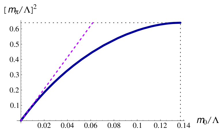
Figure 2: Pseudo-scalar meson mass squared $(m_{\pi}/\Lambda)^{2}$ as a function of $m_{0}/\Lambda$. The solid line is the numerical solution to Eq. (5.10) for $M/\Lambda=0.4$, and the dashed line is its approximate solution, Eq. (5.13). Two dotted lines are the threshold line $(2M/\Lambda)^{2}=0.64$ (horizontal) and the upper limit of the bound state $(m_{0}/\Lambda)_{\rm upper}=0.137\cdots$ (vertical) as given in Eq. (5.14).

When $m_{0}\neq 0$, the equation for the scalar meson does not have a (real) solution for $r_{\sigma}<1$ because the quantity in the curly brackets cannot be negative for $r_{\sigma}<1$. Therefore, the scalar meson does not appear as a bound state. This observation is consistent with the literature [18, 9]. On the other hand, the pseudo-scalar meson is still a bound state for small nonzero $m_{0}$ and its mass is estimated as

$$m_{\pi}^{2}=\frac{N}{g_{\rm S}}Z_{\pi}\frac{m_{0}}{M}+{\cal O}(m_{0}^{2}),\quad Z_{\pi}=\frac{1}{N}\left[\frac{1}{8\pi^{2}}\ln\frac{1+\beta}{1-\beta}-\frac{\beta}{4\pi^{2}}\right]^{-1}.$$ (5.13)

In order to compute the decay constant $f_{\pi}$, one has to determine the overall factor $C_{\pi}$ of the LC wavefunction (5.1) from Eq. (4.20). Then, one finds $f_{\pi}=2MZ_{\pi}^{-1/2}$, which, combined with Eq. (5.13), implies the Gell-Mann, Oakes, Renner relation $m_{\pi}^{2}f_{\pi}^{2}=-4m_{0}\langle\bar{\Psi}\Psi\rangle$, as was discussed in Ref. [4]. In Fig. 2, we show the numerical solution to the eigenvalue equation (5.10), together with the approximate solution (5.13). Shown is the square of the mass, and thus the linear dependence upon $m_{0}$ is clear for small $m_{0}$. As $m_{0}$ is increased, the pseudo-scalar meson’s mass increases, and reaches at the threshold $m_{\pi}=2M$. The value of bare mass $m_{0}$ which gives the threshold mass is easily calculated from Eq. (5.10) where we use $r_{\pi}=1$ and delete $g_{\rm S}$ dependence by using the gap equation. Explicitly, the result is

$$\left(\frac{m_{0}}{\Lambda}\right)_{\rm upper}={\frac{M}{\Lambda}}\left\{1+\frac{2-(M/\Lambda)^{2}(1+\ln\frac{2\Lambda^{2}}{M^{2}})}{2(M/\Lambda)^{2}\ln\frac{1+\beta}{1-\beta}}\right\}^{-1}.$$ (5.14)

For $M/\Lambda=0.4$, this upper bound of the bare mass becomes $(m_{0}/\Lambda)_{\rm upper}=0.137\cdots$, which is in agreement with the numerical result. Therefore, the bound state in the pseudo-scalar channel exists even for nonzero bare mass $m_{0}$ if it is smaller than $(m_{0}/\Lambda)_{\rm upper}$ given by Eq. (5.14).

Once we obtain the mass of mesons, we can discuss the shape of the spin-independent LC wavefunctions. It is the meson’s mass that controls the shape of wavefunction. Consider the chiral limit, only when the scalar meson appears as a bound state. Then, the difference of the mass between $m_{\pi}=0$, and $m_{\sigma}=2M$ greatly affects the shape. Both have peaks at $x=1/2$, but widths are significantly different. The wavefunction of the scalar meson has a very sharp peak at $x=1/2$ (and even divergent for $k_{\perp}=0$), which clearly shows the constituent picture. In Fig. 3, we plot $\phi(x,k_{\perp}^{2}=0.05M^{2})$’s of scalar and pseudo-scalar mesons in the chiral limit, which are compared with that of the vector meson to be derived soon. Transverse momentum has been taken nonzero in order to avoid the singular behavior at $k_{\perp}=0$. The wavefunctions are rescaled at $x=1/2$ just for comparison.

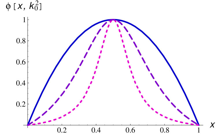
Figure 3: The spin-independent LC wavefunctions $\phi(x,k_{\perp}^{2}=0.05M^{2})$ of pseudo-scalar (solid), scalar (short-dashed) and vector (long-dashed) mesons in the chiral limit $m_{0}=0$. Mass of the vector meson is taken to be a typical value $m_{\rm V}/2M=0.9$ (see Fig. 4). Rescaled at $x=1/2$ just for comparison.

5.3 Vector mesons

We have been concerned if the bound-state equations for the transverse and longitudinal modes (Eqs. (4.27) and (4.29)) are equivalent to each other. This can be explicitly shown as follows. First of all, we can verify that both the equations (4.27) and (4.29) derive the same equation for a vector meson mass $m_{\rm V}$ with the extended parity invariant cutoff (5.4). Namely, Eq. (5.5) for the transverse and longitudinal potentials

$$V_{\rm T}=-\frac{g_{\rm V}}{(2\pi)^{3}}\frac{p_{\perp}^{2}+M^{2}-2y(1-y)p_{\perp}^{2}}{y^{2}(1-y)^{2}}\,,\qquad V_{\rm L}=-\frac{g_{\rm V}}{(2\pi)^{3}}\frac{4(p_{\perp}^{2}+M^{2})}{y(1-y)}\,,$$

leads to the same equation. This, together with the fact that the spin-independent LC wavefunctions for transverse and longitudinal modes have the same functional form (5.1), ensures the equivalence of the two bound-state equations. If the masses of transverse and longitudinal vector mesons coincide with each other, then so do the spin-independent LC wavefunctions, as well as the bound-state equations. Indeed, after some calculation, one can see that Eq. (5.5) with $i=$ T and $i=$ L reduces to the same equation for the vector meson mass $m_{\rm V}$:

$$\frac{1}{\widetilde{g}_{\rm V}}=\frac{2}{3}\left[\,\beta+(1-\beta^{2})\left\{r_{\rm V}\ln\left(\frac{1+\beta}{1-\beta}\right)-\left(2r_{\rm V}+1\right)\sqrt{\frac{1-r_{\rm V}}{r_{\rm V}}}\arctan\frac{\beta}{\sqrt{\frac{1-r_{\rm V}}{r_{\rm V}}}}\right\}\right],$$ (5.15)

where we have defined a dimensionless coupling constant $\widetilde{g}_{\rm V}=({\Lambda^{2}}/{4\pi^{2}})\,g_{\rm V}$ and $r_{\rm V}$ similarly as for the scalar and pseudo-scalar cases:

$$r_{\rm V}\equiv\left(\frac{m_{\rm V}}{2M}\right)^{2}.$$ (5.16)

This completes the proof of the equivalence between the transverse and longitudinal equations.

Let us consider the physics consequences of the eigenvalue equation (5.15). A physical bound-state should appear only when the ratio $r_{\rm V}$ is in the range $0<r_{\rm V}<1$. Equation (5.15) has a solution in this region when the strength of the coupling constant $\widetilde{g}_{\rm V}$ is in the range $\widetilde{g}_{\rm V}^{\rm{(min)}}<\widetilde{g}_{\rm V}<\widetilde{g}_{\rm V}^{\rm{(max)}}$ defined by

$$\widetilde{g}_{\rm V}^{\rm{(min)}}\equiv\frac{3}{2}\left\{\beta+(1-\beta^{2})\ln\left(\frac{1+\beta}{1-\beta}\right)\right\}^{-1},\quad\widetilde{g}_{\rm V}^{\rm{(max)}}\equiv\frac{3}{2}\cdot\frac{1}{\beta^{3}}\,.$$ (5.17)

Two limiting cases $\widetilde{g}_{\rm V}=\widetilde{g}_{\rm V}^{\rm{(min)}}$ and $\widetilde{g}_{\rm V}=\widetilde{g}_{\rm V}^{\rm{(max)}}$ correspond to $r_{\rm V}=1$ (loose binding limit), and $r_{\rm V}=0$ (tight binding limit), respectively. When $M/\Lambda\rightarrow 0\ (\beta\to 1)$, the physical bound-state region shrinks $\widetilde{g}_{\rm V}^{\rm{(min)}}\rightarrow\widetilde{g}_{\rm V}^{\rm{(max)}}$, while it becomes wider as $M/\Lambda$ grows large. The existence of $\widetilde{g}_{\rm V}^{\rm(min)}$ is consistent with the observation that there is no bound state in the NJL model without the vector interaction. Similar behaviors have been found in Ref. [19].

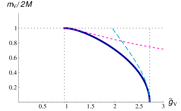
Figure 4: Vector meson’s mass $m_{\rm V}/2M$ as a function of $\widetilde{g}_{\rm V}$. The numerical solution to Eq. (5.15) (solid line) is compared with its approximate solutions Eq. (5.18) (short-dashed) and Eq. (5.19) (long-dashed). Constituent quark mass is taken to be $M/\Lambda=0.4$ (see Fig. 1). A bound state appears only in the regime $\widetilde{g}_{\rm V}^{\rm{(min)}}=0.95\ <\widetilde{g}_{\rm V}<\widetilde{g}_{\rm V}^{\rm{(max)}}=2.72$, which are indicated by two vertical dotted lines. The horizontal dotted line corresponds to the threshold.

One can find approximate solutions to Eq. (5.15) when the vector coupling $\widetilde{g}_{\rm V}$ is close to either its minimum $\widetilde{g}_{\rm V}^{\rm{(min)}}$ or maximum $\widetilde{g}_{\rm V}^{\rm{(max)}}$. Namely,

$$r_{\rm V} \simeq 1-\left\{\frac{({\widetilde{g}^{\rm(min)}_{\rm V}})^{-1}-({\widetilde{g}_{\rm V}})^{-1}}{\pi(1-\beta^{2})}\right\}^{2}\qquad\ {\rm for}\qquad\widetilde{g}_{\rm V}\mathrel{\hbox to0.0pt{\raise 2.20013pt\hbox{$>$}\hss}{\lower 2.20013pt\hbox{$\sim$}}}\widetilde{g}^{\rm(min)}_{\rm V}\,,$$ (5.18)

$$r_{\rm V} \simeq \frac{({\widetilde{g}_{\rm V}})^{-1}-({\widetilde{g}^{\rm(max)}_{\rm V}})^{-1}}{\frac{2}{3}(1-\beta^{2})\left(\ln\frac{1+\beta}{1-\beta}-2\beta\right)}\qquad\qquad{\rm for}\qquad\widetilde{g}_{\rm V}\mathrel{\hbox to0.0pt{\raise 2.20013pt\hbox{$<$}\hss}{\lower 2.20013pt\hbox{$\sim$}}}\widetilde{g}^{\rm(max)}_{\rm V}\,.$$ (5.19)

When we derived the bound-state equations (4.27) and (4.29), we picked up the leading contribution in the (integral form of the) eigen-value equation for $m_{\rm V}$ (see Appendix F). However, the solution to the resulting eigen-value equation (5.15) has highly nontrivial dependence upon $\widetilde{g}_{\rm V}$. This is evident in the above approximate solutions to the equation.

In Fig. 4, a numerical solution to Eq. (5.15) is shown as a function of $\widetilde{g}_{\rm V}$, where the constituent quark mass is taken to be $M/\Lambda=0.4\ (\beta=0.82)$ as an example. As we expect, a bound state appears for $\widetilde{g}_{\rm V}$ larger than the critical value $\widetilde{g}^{\rm(min)}_{\rm V}$, and as one increases $\widetilde{g}_{\rm V}$, the mass starts to decrease from the threshold value $2M$. The value of critical coupling constants are exactly the same as the values predicted by the analytic calculation. When $\beta=0.82$, they are $\widetilde{g}_{\rm V}^{\rm{(min)}}=0.95$ and $\widetilde{g}_{\rm V}^{\rm{(max)}}=2.72$, which are indicated as two vertical dotted lines in the figure. Besides, we have plotted the approximate solutions Eqs. (5.18) and (5.19) in the same figure, and they are in good agreement in the regimes where each approximation is valid.

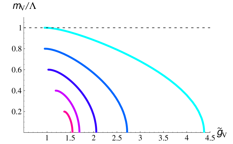
Figure 5: Vector meson’s mass $m_{\rm V}/\Lambda$ as a function of $\widetilde{g}_{\rm V}$ for different values of constituent mass $M/\Lambda$. From bottom to top, $M/\Lambda=0.1,\,0.2,\,0.3,\,0.4,\,0.5.$ The line for $M/\Lambda=0.4$ is the same result as shown in Fig. 4. Below the dashed line is the physical region. These results can be re-interpreted as either $m_{0}$ or $\widetilde{g}_{\rm S}$ dependences from Fig. 1, since the $m_{0}$ and $\widetilde{g}_{\rm S}$ dependences enter the vector meson’s mass only through the constituent mass $M$.

It is also interesting to see $m_{\rm V}$ as a function of $\widetilde{g}_{\rm V}$ for different values of the constituent mass. This is shown in Fig. 5. Unlike in Fig. 4, the vertical axis is $m_{\rm V}/\Lambda$ instead of $m_{\rm V}/2M$ since we change the value of constituent mass $M/\Lambda=0.1\sim 0.5$. Though the eigenvalue equation (5.15) does not explicitly depend upon $\widetilde{g}_{\rm S}$ and $m_{0}$, they indirectly affect the vector meson’s mass through the constituent mass $M$ (cf. Fig. 1). Thus, to study the $M$ dependence of $m_{\rm V}$ also implies to study the $\widetilde{g}_{\rm S}$ or $m_{0}$ dependence. The result in Fig. 5 is consistent with the 3 dimensional plot of $m_{\rm V}/\Lambda$ as a function of $\widetilde{g}_{\rm V}$ and $\widetilde{g}_{\rm S}$ in the chiral limit, which was presented in the letter [10]. As $M/\Lambda$ is increased (i.e., going to larger $\widetilde{g}_{\rm S}$), the bound-state region becomes larger as was discussed around Eq. (5.17).

Lastly, we compare the spin-independent LC wavefunction of the vector meson with those of the scalar and pseudo-scalar mesons. This is shown in Fig. 3 as already mentioned. We plot three wavefunctions for nonzero transverse momentum $k_{\perp}^{2}=0.05M^{2}$ in the chiral limit $m_{0}=0$. Mass of the vector meson is taken to be a typical value $m_{\rm V}/2M=0.9$ (see Fig. 4). All the wavefunctions are normalized at $x=1/2$ for comparison. As we discussed before, the difference of shape is due to different values of the mass. In the chiral limit, we have a relation $0=m_{\pi}\leq m_{\rm V}\leq m_{\sigma}=2M$. Thus it is reasonable that the wavefunction of the vector meson lies in between those of the scalar and pseudo-scalar mesons. The constituent picture works better for a vector meson than for a pseudo-scalar meson.

6 Summary and discussions

We have presented a detailed analysis of the application of light-front quantization to light mesons. Our framework is one of the most straightforward approaches towards relativistic bound-state systems, and indeed allows us to obtain the light-cone wavefunction and mass of the meson simultaneously by solving the Hamiltonian eigenvalue equation. One of the subtleties in treating light mesons in the light-front formalism is the chiral symmetry breaking. However, we know how to describe it at least in the Nambu-Jona-Lasinio model as discussed in the present paper. All the calculation was done within the NJL model with the vector interaction and in the large $N$ limit, where a meson is described as a composite state of a quark and an antiquark. We mainly focused on the problems of describing vector mesons and understanding their properties, though we also reproduced the previous results for the scalar and pseudo-scalar mesons in Ref. [4]. The vector mesons can be formed in the NJL model if one adds the vector interaction which strengthens the attractive force between the quark and the antiquark. For the light mesons, the effect of chiral symmetry breaking is of special importance. We followed the same procedures as in Ref. [4] to incorporate this effect. We are able to obtain the LC Hamiltonian in the broken phase, which then can be used in deriving the bound-state equations. In the NJL model, we have to be careful about the regularization scheme, but once it is properly done, we can obtain reasonable results about the LC wavefunctions and masses of light mesons. Mass of the vector meson decreases as one increases the strength of the vector interaction. This behavior is consistent with Refs.[19, 20] which also treated the vector meson within the NJL model with the vector interaction.

We utilized several approximations in deriving the bound-state equations. For the vector meson, we estimated only the leading effect with respect to the vector coupling. In fact, this was enough to form a bound state in the vector channel, but somewhat unexpected behavior of the mass that it vanishes at some critical vector coupling $\widetilde{g}^{\rm(max)}_{\rm V}$, is probably due to this approximation. For the scalar and pseudo-scalar mesons, we ignored the effects of vector interaction, because bound states are possible even with the scalar interaction. We know that the vector interaction can modify the structure of pseudo-scalar mesons, and it would be important to study this effect.

The methods we developed in the present paper seems specific to the NJL model. This is not true. Actually, the applicability of the formalism is not limited to the NJL model, but is much wider. For example, the same formalism can be applied to any fermionic models without gauge fields, which include models with nonlocal current-current interaction generated by either one gluon exchange or instantons.

There remain several interesting topics to be considered in the future. First, now that we obtain the LC wavefunctions of light mesons, we can use them to compute the physical observables such as the distribution amplitudes. Of special importance is the physical form factors. Such analysis was indeed done for a pseudo-scalar meson [15], but a similar analysis is possible for the vector meson [21]. Next, our framework can in principle treat the axial vector state in a similar way, and it would be interesting to investigate its bound-state structure.

Appendix A Notations

Our notation is the following: The light-cone coordinates are $x^{\pm}=(x^{0}\pm x^{3})/\sqrt{2},$ and $x_{\perp}^{i}=(x^{1},x^{2})=\vec{x}_{\perp}$, which are written together as $x^{\mu}=(x^{+},x^{-},x_{\perp}^{i})$. The derivatives are $\partial_{\pm}=\partial/\partial x^{\pm}$ and $\partial_{\perp}=\partial/\partial x_{\perp}$. We define the spatial vector $x$ for coordinates by $\mbox{\boldmath{$x$}}=(x^{-},x_{\perp}^{i})$. On the other hand, for momenta, we define $\mbox{\boldmath{$p$}}=(p^{+},p^{1}_{\perp},p^{2}_{\perp})$ (notice that $p^{+}=p_{-}$ is conjugate to $x^{-}$) and $\mbox{\boldmath{$p$}}\mbox{\boldmath{$x$}}=-p^{+}x^{-}+p_{\perp}^{i}x_{\perp}^{i}$ so that $px=p^{-}x^{+}+p^{+}x^{-}-p_{\perp}^{i}x_{\perp}^{i}=p^{-}x^{+}-\mbox{\boldmath{$p$}}\mbox{\boldmath{$x$}}$. We use $\mu,\nu$ for Lorentz indices of four vectors, $i,j$ for transverse coordinates $1,2,$ and $\alpha,\beta$ for spinor indices.

The projection operator $\Lambda_{\pm}$ is defined by

$$\Lambda_{\pm}\equiv\frac{1}{2}(1\pm\gamma^{0}\gamma^{3})$$ (A.1)

and satisfies $(\Lambda_{\pm})^{2}=\Lambda_{\pm}$, and $\Lambda_{+}+\Lambda_{-}=1$. Some useful formulas are $\Lambda_{-}\gamma^{+}=\gamma^{+}\Lambda_{+}$, $\Lambda_{+}\gamma^{-}=\gamma^{-}\Lambda_{-}$.

Appendix B LF Quantization of a free fermion: spinor basis

Here we summarize the LF quantization of a free fermion based on the plane wave solutions to the Dirac equation. This gives our ”spinor basis” which is useful when we treat the case with vector interaction.

Consider a classical plane wave solution $\psi(x)=u(p)\,{\rm e}^{-ipx}$ to the free Dirac equation:

$$(\gamma^{\mu}p_{\mu}-M)u(p)=0\,,\hskip 56.9055pt(\mu=+,-,1,2)$$ (B.1)

where the four momentum $p^{\mu}$ must satisfy the dispersion relation

$$p^{-}=\frac{{p}_{\perp}^{2}+M^{2}}{2p^{+}}.$$ (B.2)

So far, the LC energy $p^{-}$ can take either positive or negative value, but, we redefine the negative energy solution $u(-p^{-},-p^{+},-p_{\perp})$ ($p^{-}>0,\ p^{+}>0$) by $v(p^{-},p^{+},p_{\perp})$, and we always treat $p^{-}$ to be positive. We call $u(\mbox{\boldmath{$p$}})$ and $v(\mbox{\boldmath{$p$}})$ the positive and negative energy solutions, respectively. It should be noticed that the longitudinal momentum $p^{+}$ is also positive, because the sign of the LC energy and that of the longitudinal momentum is correlated as is shown in Eq. (B.2). The ”positive energy solution” $u(p^{+},{p}_{\perp},s)$ satisfies $0=(\gamma^{\mu}p_{\mu}-M)\,u(p^{+},{p}_{\perp},s)$ and ${\bar{u}(p^{+},{p}_{\perp},s)}\,(\gamma^{\mu}p_{\mu}-M)=0,$ where $s$ is an index to distinguish two different solutions. Similarly, the ”negative energy solution” $v(p^{+},{p}_{\perp},s)$ satisfies $0=(-\gamma^{\mu}p_{\mu}-M)\ v(p^{+},{p}_{\perp},s)$ and ${\bar{v}(p^{+},{p}_{\perp},s)}\,(-\gamma^{\mu}p_{\mu}-M)=0.$ Normalization of the solutions are given by

$${\bar{u}}(\mbox{\boldmath{$p$}},s)\,u(\mbox{\boldmath{$p$}},s^{\prime})=-{\bar{v}}(\mbox{\boldmath{$p$}},s)\,v(\mbox{\boldmath{$p$}},s^{\prime})=2\,M\,\delta_{ss^{\prime}}\,,$$

and the followings are useful:

$${\bar{u}}(\mbox{\boldmath{$p$}},s)\gamma^{\mu}\,u(\mbox{\boldmath{$p$}},s^{\prime}) = {\bar{v}}(\mbox{\boldmath{$p$}},s)\gamma^{\mu}\,v(\mbox{\boldmath{$p$}},s^{\prime})=2\,p^{\mu}\,\delta_{ss^{\prime}},$$

$$\sum_{s}u(\mbox{\boldmath{$p$}},s)\,{\bar{u}}(\mbox{\boldmath{$p$}},s) = p_{\mu}\gamma^{\mu}+M,$$

$$\sum_{s}v(\mbox{\boldmath{$p$}},s)\,{\bar{v}}(\mbox{\boldmath{$p$}},s) = p_{\mu}\gamma^{\mu}-M.$$

The fermion field can be expanded by use of these complete solutions,

$$\psi(x) = \frac{1}{\left(2\pi\right)^{3/2}}\int_{0}^{\infty}dp^{+}\int_{-\infty}^{\infty}d^{2}{p}_{\perp}\frac{1}{\sqrt{2p^{+}}}$$ (B.3)

$$\times\sum_{s=\pm}\left[b(p^{+},{p}_{\perp},s)\ u(p^{+},{p}_{\perp},s)\,{\rm e}^{-ip\cdot x}+d^{\dagger}(p^{+},{p}_{\perp},s)\ v(p^{+},{p}_{\perp},s)\,{\rm e}^{ip\cdot x}\right],$$

where $b(p^{+},{p}_{\perp},s)$ and $d^{\dagger}(p^{+},{p}_{\perp},s)$ are c-number coefficients. Defining $\psi=\Lambda_{+}\psi+\Lambda_{-}\psi\equiv\psi_{+}+\psi_{-},$ the good component $\psi_{+}$ is expanded as

$$\psi_{+}(x) = \frac{1}{\left(2\pi\right)^{3/2}}\int_{0}^{\infty}dp^{+}\int_{-\infty}^{\infty}d^{2}{p}_{\perp}\frac{1}{\sqrt{2p^{+}}}$$ (B.4)

$$\times\sum_{s=\pm}\left[b(p^{+},{p}_{\perp},s)\ u_{+}(p^{+},{p}_{\perp},s)\,{\rm e}^{-ip\cdot x}+d^{\dagger}(p^{+},{p}_{\perp},s)\ v_{+}(p^{+},{p}_{\perp},s)\,{\rm e}^{ip\cdot x}\right],$$

where $u_{+}=\Lambda_{+}u$ and $v_{+}=\Lambda_{+}v$. These projected spinors satisfy the following relations:

$$u_{+}^{\dagger}(\mbox{\boldmath{$p$}},s^{\prime})u_{+}(\mbox{\boldmath{$p$}},s) = v_{+}^{\dagger}(\mbox{\boldmath{$p$}},s^{\prime})v_{+}(\mbox{\boldmath{$p$}},s)=\sqrt{2}p^{+}\,\delta_{ss^{\prime}}$$

$$\sum_{s}u_{+}(\mbox{\boldmath{$p$}},s)u_{+}^{\dagger}(\mbox{\boldmath{$p$}},s) = \sum_{s}v_{+}(\mbox{\boldmath{$p$}},s)v_{+}^{\dagger}(\mbox{\boldmath{$p$}},s)=\sqrt{2}\Lambda_{+}p^{+}\,\,.$$

Since $\psi_{-}$ is a dependent variable, we impose the quantization condition only on the good component $\psi_{+}$ (see Eqs. (2.5), (2.6)). The mode expansion for $\psi_{+}$ is given in the same form as Eq. (B.4), but now $b(p^{+},{p}_{\perp},s)$ and $d^{\dagger}(p^{+},{p}_{\perp},s)$ are operators.

The mode expansion of the bad component $\psi_{-}$ should be given through the constraint equation $\psi_{-}(x)=\frac{1}{2i\partial_{-}}(i\gamma_{\perp}^{i}\partial_{i}+M)\gamma^{+}\psi_{+}$ by using Eq. (B.4). One can explicitly show that $\psi=\psi_{+}+\psi_{-}$ reproduces the mode expansion Eq. (B.3).

Appendix C Boson expansion method as the $1/N$ expansion of ${\sf M}(\mbox{\boldmath{$p$}},\mbox{\boldmath{$q$}})$

In the boson expansion method, we rewrite the bilocal operators ${\sf M}(\mbox{\boldmath{$p$}},\mbox{\boldmath{$q$}})$ defined by Eq. (3.1) with respect to bosonic operators so that the commutation relation between ${\sf M}(\mbox{\boldmath{$p$}},\mbox{\boldmath{$q$}})$’s is correctly reproduced. Physically this corresponds to capturing a composite state made of a fermion and an antifermion, as a bosonic state with additional ”structure” due to statistics. Especially, when $N$ is large, the composite state behaves as a boson, and thus large $N$ expansion of the bilocal operator is naturally realized by the boson expansion method (of the Holstein-Primakoff type).

The bilocal operator ${\sf M}(\mbox{\boldmath{$p$}},\mbox{\boldmath{$q$}})$ satisfies the following commutator:

$$\Big{[}:{\sf M}_{\alpha_{1}\alpha_{2}}(\mbox{\boldmath{$p$}}_{1},\mbox{\boldmath{$p$}}_{2}):\,,\ \ :{\sf M}_{\beta_{1}\beta_{2}}(\mbox{\boldmath{$q$}}_{1},\mbox{\boldmath{$q$}}_{2}):\Big{]}$$ (C.1)

$$=\,:{\sf M}_{\alpha_{1}\beta_{2}}(\mbox{\boldmath{$p$}}_{1},\mbox{\boldmath{$q$}}_{2}):(\Lambda_{+})_{\alpha_{2}\beta_{1}}\delta(\mbox{\boldmath{$p$}}_{2}+\mbox{\boldmath{$q$}}_{1})\,-\,:{\sf M}_{\beta_{1}\alpha_{2}}(\mbox{\boldmath{$q$}}_{1},\mbox{\boldmath{$p$}}_{2}):(\Lambda_{+})_{\beta_{2}\alpha_{1}}\delta(\mbox{\boldmath{$q$}}_{2}+\mbox{\boldmath{$p$}}_{1})$$

$$\quad+\,N(\Lambda_{+})_{\beta_{2}\alpha_{1}}\delta(\mbox{\boldmath{$q$}}_{2}+\mbox{\boldmath{$p$}}_{1})(\Lambda_{+})_{\alpha_{2}\beta_{1}}\delta(\mbox{\boldmath{$p$}}_{2}+\mbox{\boldmath{$q$}}_{1})$$

$$\times\Big{(}\theta(p_{1}^{+})\theta(p_{2}^{+})\theta(-q_{1}^{+})\theta(-q_{2}^{+})-\theta(-p_{1}^{+})\theta(-p_{2}^{+})\theta(q_{1}^{+})\theta(q_{2}^{+})\Big{)},$$

and its vacuum expectation value is

$$\langle 0|{\sf M}_{\alpha\beta}(\mbox{\boldmath{$p$}},\mbox{\boldmath{$q$}})|0\rangle=N\theta(p^{+})\delta(\mbox{\boldmath{$p$}}+\mbox{\boldmath{$q$}})(\Lambda_{+})_{\beta\alpha}.$$ (C.2)

This complicated commutator can be reproduced by replacing ${\sf M}(\mbox{\boldmath{$p$}},\mbox{\boldmath{$q$}})$ by some simple functions of a (bilocal) bosonic operator.

Let us first introduce bilocal bosonic operators $B_{\alpha\beta}(\mbox{\boldmath{$p$}},\mbox{\boldmath{$q$}})$ which have Dirac indices. We impose they satisfy the following commutation relations:

$$[B_{\alpha_{1}\alpha_{2}}(\mbox{\boldmath{$p$}}_{1},\mbox{\boldmath{$p$}}_{2}),\,B_{\beta_{1}\beta_{2}}^{\dagger}(\mbox{\boldmath{$q$}}_{1},\mbox{\boldmath{$q$}}_{2})]=(\Lambda_{+})_{\alpha_{1}\beta_{1}}\delta(\mbox{\boldmath{$p$}}_{1}-\mbox{\boldmath{$q$}}_{1})(\Lambda_{+})_{\beta_{2}\alpha_{2}}\delta(\mbox{\boldmath{$q$}}_{2}-\mbox{\boldmath{$p$}}_{2}),$$ (C.3)

$$[{B}_{\alpha_{1}\alpha_{2}}(\mbox{\boldmath{$p$}}_{1},\mbox{\boldmath{$p$}}_{2}),{B}_{\beta_{1}\beta_{2}}(\mbox{\boldmath{$q$}}_{1},\mbox{\boldmath{$q$}}_{2})]=0\qquad(p_{i}^{+},q_{i}^{+}>0),$$ (C.4)

and the following properties

$$(\Lambda_{+})_{\alpha_{1}\gamma_{1}}B_{\gamma_{1}\gamma_{2}}(\mbox{\boldmath{$p$}}_{1},\mbox{\boldmath{$p$}}_{2})=B_{\alpha_{1}\gamma_{2}}(\mbox{\boldmath{$p$}}_{1},\mbox{\boldmath{$p$}}_{2}),\hskip 14.22636ptB_{\gamma_{1}\gamma_{2}}(\mbox{\boldmath{$p$}}_{1},\mbox{\boldmath{$p$}}_{2})(\Lambda_{+})_{\gamma_{2}\alpha_{2}}=B_{\gamma_{1}\alpha_{2}}(\mbox{\boldmath{$p$}}_{1},\mbox{\boldmath{$p$}}_{2})\,,$$ (C.5)

$$(\Lambda_{+})_{\gamma_{1}\alpha_{1}}B^{\dagger}_{\gamma_{1}\gamma_{2}}(\mbox{\boldmath{$p$}}_{1},\mbox{\boldmath{$p$}}_{2})=B^{\dagger}_{\alpha_{1}\gamma_{2}}(\mbox{\boldmath{$p$}}_{1},\mbox{\boldmath{$p$}}_{2}),\hskip 14.22636ptB^{\dagger}_{\gamma_{1}\gamma_{2}}(\mbox{\boldmath{$p$}}_{1},\mbox{\boldmath{$p$}}_{2})(\Lambda_{+})_{\alpha_{2}\gamma_{2}}=B^{\dagger}_{\gamma_{1}\alpha_{2}}(\mbox{\boldmath{$p$}}_{1},\mbox{\boldmath{$p$}}_{2})\,,$$ (C.6)

and so on. Then the operators $:{\sf M}:$ can be represented as

$$:{\sf M}^{-+}_{\alpha_{1}\alpha_{2}}(\mbox{\boldmath{$p$}}_{1},\mbox{\boldmath{$p$}}_{2}): = \int_{0}^{\infty}dq^{+}\int_{-\infty}^{\infty}d^{2}q_{\perp}B^{\dagger}_{\alpha_{1}\gamma}(-\mbox{\boldmath{$p$}}_{1},\mbox{\boldmath{$q$}})B_{\alpha_{2}\gamma}(\mbox{\boldmath{$p$}}_{2},\mbox{\boldmath{$q$}})$$ (C.7)

$$\equiv {\cal A}_{\alpha_{2}\alpha_{1}}(\mbox{\boldmath{$p$}}_{2},-\mbox{\boldmath{$p$}}_{1}),$$

$$:{\sf M}^{+-}_{\alpha_{1}\alpha_{2}}(\mbox{\boldmath{$p$}}_{1},\mbox{\boldmath{$p$}}_{2}): = -\int_{0}^{\infty}dq^{+}\int_{-\infty}^{\infty}d^{2}q_{\perp}B^{\dagger}_{\gamma\alpha_{2}}(\mbox{\boldmath{$q$}},-\mbox{\boldmath{$p$}}_{2})B_{\gamma\alpha_{1}}(\mbox{\boldmath{$q$}},\mbox{\boldmath{$p$}}_{1}),$$ (C.8)

$$:{\sf M}^{++}_{\alpha_{1}\alpha_{2}}(\mbox{\boldmath{$p$}}_{1},\mbox{\boldmath{$p$}}_{2}): = \int_{0}^{\infty}dq^{+}\int_{-\infty}^{\infty}d^{2}q_{\perp}(\sqrt{N-{\cal A}})_{\alpha_{2}\gamma}(\mbox{\boldmath{$p$}}_{2},\mbox{\boldmath{$q$}})B_{\gamma\alpha_{1}}(\mbox{\boldmath{$q$}},\mbox{\boldmath{$p$}}_{1}),$$ (C.9)

$$:{\sf M}^{--}_{\alpha_{1}\alpha_{2}}(\mbox{\boldmath{$p$}}_{1},\mbox{\boldmath{$p$}}_{2}): = \int_{0}^{\infty}dq^{+}\int_{-\infty}^{\infty}d^{2}q_{\perp}B^{\dagger}_{\gamma\alpha_{2}}(\mbox{\boldmath{$q$}},-\mbox{\boldmath{$p$}}_{2})(\sqrt{N-{\cal A}})_{\gamma\alpha_{1}}(\mbox{\boldmath{$q$}},-\mbox{\boldmath{$p$}}_{1}),$$ (C.10)

where the upper indices stand for the signs of the longitudinal momenta. This is the boson expansion method of the Holstein-Primakoff type, represented in the ”Dirac basis” (namely, the bosonic operators explicitly have the Dirac indices). This is essentially the same as the one used in Ref. [4]. Note that the bosonic operator is of ${\cal O}(N^{0})$, and there is explicit dependence on $N$ on the right-hand sides. Thus, one can expand the right-hand sides with respect to $1/\sqrt{N}$, yielding Eq. (3.6) in the text. It should be noticed that the natural expansion parameter is $1/\sqrt{N}$ instead of $1/N$ because we have expanded $\sqrt{1-{\cal A}/N}$. The first few terms are given as follows:

$${\sf m}_{\alpha\beta}^{(0)}(\mbox{\boldmath{$p$}},{\mbox{\boldmath{$q$}}}) = (\Lambda_{+})_{\beta\alpha}\delta(\mbox{\boldmath{$p$}}+{\mbox{\boldmath{$q$}}})\theta(p^{+})\theta(-q^{+})~{},$$ (C.11)

$${\sf m}_{\alpha\beta}^{(1)}(\mbox{\boldmath{$p$}},{\mbox{\boldmath{$q$}}}) = B_{\beta\alpha}({\mbox{\boldmath{$q$}}},\mbox{\boldmath{$p$}})\theta(p^{+})\theta(q^{+})+B_{\alpha\beta}^{\dagger}(-\mbox{\boldmath{$p$}},-\mbox{\boldmath{$q$}})\theta(-p^{+})\theta(-q^{+})~{},$$ (C.12)

$${\sf m}_{\alpha\beta}^{(2)}(\mbox{\boldmath{$p$}},\mbox{\boldmath{$q$}}) = \int[d\mbox{\boldmath{$k$}}]\,B^{\dagger}_{\alpha\gamma}(-\mbox{\boldmath{$p$}},\mbox{\boldmath{$k$}})B_{\beta\gamma}(\mbox{\boldmath{$q$}},\mbox{\boldmath{$k$}})\theta(-p^{+})\theta(q^{+})$$ (C.13)

$$- \int[d\mbox{\boldmath{$k$}}]\,B^{\dagger}_{\gamma\beta}(\mbox{\boldmath{$k$}},-\mbox{\boldmath{$q$}})B_{\gamma\alpha}(\mbox{\boldmath{$k$}},\mbox{\boldmath{$p$}})\theta(p^{+})\theta(-q^{+})~{}.$$

The leading term ${\sf m}_{\alpha\beta}^{(0)}(\mbox{\boldmath{$p$}},\mbox{\boldmath{$q$}})$ comes from the vacuum expectation value of ${\sf M}(\mbox{\boldmath{$p$}},\mbox{\boldmath{$q$}})$. The result ${\sf m}_{\alpha\beta}^{(1)}(\mbox{\boldmath{$p$}},{\mbox{\boldmath{$q$}}})$ means that the bilocal operator ${\sf M}(\mbox{\boldmath{$p$}},\mbox{\boldmath{$q$}})$ can be treated as a bosonic operator in the first nontrivial leading order.

One can further introduce bilocal bosonic operators $B(\mbox{\boldmath{$p$}}_{1},s_{1}:\mbox{\boldmath{$p$}}_{2},s_{2})$ in the ”spinor basis”, namely, with spins instead of simple Dirac indices. The relation between operators in the ”Dirac basis” and in the ”spinor basis” is given by

$$B_{\alpha_{1}\alpha_{2}}(\mbox{\boldmath{$p$}}_{1},\mbox{\boldmath{$p$}}_{2})=\frac{1}{\sqrt{2p_{1}^{+}p_{2}^{+}}}\sum_{s_{1}=\pm}\sum_{s_{2}=\pm}u_{+\alpha_{1}}(\mbox{\boldmath{$p$}}_{1},s_{1})v^{\dagger}_{+\alpha_{2}}(\mbox{\boldmath{$p$}}_{2},s_{2})B(\mbox{\boldmath{$p$}}_{1},s_{1}:\mbox{\boldmath{$p$}}_{2},s_{2})\,,$$ (C.14)

where the good components of the spinor $u_{+}=\Lambda_{+}u$ and $v_{+}=\Lambda_{+}v$ are introduced in Appendix B. The operator $B(\mbox{\boldmath{$p$}}_{1},s_{1}:\mbox{\boldmath{$p$}}_{2},s_{2})$ satisfies a very simple commutator (as shown in the text):

$$[B(\mbox{\boldmath{$p$}}_{1},s_{1}:\mbox{\boldmath{$p$}}_{2},s_{2}),B^{\dagger}(\mbox{\boldmath{$p$}}^{\prime}_{1},s_{1}^{{}^{\prime}}:\mbox{\boldmath{$p$}}^{\prime}_{2},s_{2}^{{}^{\prime}})]=\delta_{s_{1}s_{1}^{{}^{\prime}}}\delta(\mbox{\boldmath{$p$}}_{1}-\mbox{\boldmath{$p$}}^{\prime}_{1})\delta_{s_{2}s_{2}^{{}^{\prime}}}\delta(\mbox{\boldmath{$p$}}_{2}-\mbox{\boldmath{$p$}}^{\prime}_{2})\,.$$

Appendix D Higher order solutions to the fermionic constraint and the LC Hamiltonian in the case without vector interaction

D.1 Higher order solutions

The bilocal fermionic constraints (3.4) and (3.5) for the higher orders can be cast into a compact form similar to that of the lowest order:

$$\pmatrix{{\sf s}^{(n)}(\mbox{\boldmath{$p$}},\mbox{\boldmath{$q$}})\cr{\sf p}^{(n)}(\mbox{\boldmath{$p$}},\mbox{\boldmath{$q$}})}=\pmatrix{F^{(n)}(\mbox{\boldmath{$p$}},\mbox{\boldmath{$q$}})\cr G^{(n)}(\mbox{\boldmath{$p$}},\mbox{\boldmath{$q$}})}-g_{\rm S}\frac{\epsilon(p^{+})}{q^{+}}\int_{-\infty}^{\infty}\frac{d^{3}\mbox{\boldmath{$k$}}}{(2\pi)^{3}}\pmatrix{{\sf s}^{(n)}(\mbox{\boldmath{$k$}},\mbox{\boldmath{$p$}}+\mbox{\boldmath{$q$}}-\mbox{\boldmath{$k$}})\cr{\sf p}^{(n)}(\mbox{\boldmath{$k$}},\mbox{\boldmath{$p$}}+\mbox{\boldmath{$q$}}-\mbox{\boldmath{$k$}})}\,,$$ (D.1)

where $F^{(n)}$ and $G^{(n)}$ are known functions expressed by ${\sf m}^{(n)}$ and lower order quantities ${\sf s}^{(m)}$, ${\sf p}^{(m)}$ and ${\sf m}^{(m)}$ with $m<n$. For example, in the next leading order ${\cal O}(\sqrt{N})$ with $n=1$:

$$\pmatrix{F^{(1)}(\mbox{\boldmath{$p$}},\mbox{\boldmath{$q$}})\cr G^{(1)}(\mbox{\boldmath{$p$}},\mbox{\boldmath{$q$}})}=\left(\pmatrix{1\cr-i\gamma_{5}}\frac{(\gamma^{i}q_{\perp}^{i}+M)}{2q^{+}}\right)_{\alpha\beta}{\sf m}^{(1)}_{\alpha\beta}(\mbox{\boldmath{$p$}},\mbox{\boldmath{$q$}})-\left(\frac{(\gamma^{i}q_{\perp}^{i}+M)}{2q^{+}}\pmatrix{1\cr i\gamma_{5}}\right)_{\alpha\beta}{\sf m}^{(1)}_{\alpha\beta}(\mbox{\boldmath{$q$}},\mbox{\boldmath{$p$}}),$$ (D.2)

and in the next-to-next leading order ${\cal O}(N^{0})$ with $n=2$, one finds

$$F^{(2)}(\mbox{\boldmath{$p$}},\mbox{\boldmath{$q$}}) = \frac{(\gamma^{i}q_{\perp}^{i}+M)_{\alpha\beta}}{2q^{+}}\left\{{\sf m}^{(2)}_{\alpha\beta}(\mbox{\boldmath{$p$}},\mbox{\boldmath{$q$}})-{\sf m}^{(2)}_{\alpha\beta}(\mbox{\boldmath{$q$}},\mbox{\boldmath{$p$}})\right\}$$ (D.3)

$$\hskip 14.22636pt-\frac{g_{\rm S}}{2q^{+}}\int\frac{d^{3}\mbox{\boldmath{$k$}}d^{3}{\mbox{\boldmath{$\l$}}}}{(2\pi)^{3}}\left\{{\sf m}^{(1)}_{\alpha\beta}(\mbox{\boldmath{$p$}},\mbox{\boldmath{$q$}}-\mbox{\boldmath{$k$}}-\mbox{\boldmath{$\l$}})\,\left[{\sf s}^{(1)}+i\gamma_{5}~{}{\sf p}^{(1)}\right]_{\alpha\beta}(\mbox{\boldmath{$k$}},\mbox{\boldmath{$\l$}})\right.$$

$$\hskip 56.9055pt\left.-\left[{\sf s}^{(1)}-i\gamma_{5}~{}{\sf p}^{(1)}\right]_{\alpha\beta}(\mbox{\boldmath{$k$}},\mbox{\boldmath{$\l$}})\,{\sf m}^{(1)}_{\alpha\beta}(\mbox{\boldmath{$q$}}-\mbox{\boldmath{$k$}}-\mbox{\boldmath{$\l$}},\mbox{\boldmath{$p$}})\right\}~{},$$

and similarly for $G^{(2)}$.

The integral equation (D.1) has a very simple structure. One can solve it by integrating the equation so that the integral on the left-hand side becomes the same as the second term in (D.1). Namely, the solution is

$$\pmatrix{{\sf s}^{(n)}(\mbox{\boldmath{$p$}},\mbox{\boldmath{$q$}})\cr{\sf p}^{(n)}(\mbox{\boldmath{$p$}},\mbox{\boldmath{$q$}})}=\pmatrix{F^{(n)}(\mbox{\boldmath{$p$}},\mbox{\boldmath{$q$}})\cr G^{(n)}(\mbox{\boldmath{$p$}},\mbox{\boldmath{$q$}})}-g_{\rm S}\kappa_{\rm S}\frac{\epsilon(p^{+})}{q^{+}}\int_{-\infty}^{\infty}\frac{d^{3}\mbox{\boldmath{$k$}}}{(2\pi)^{3}}\pmatrix{F^{(n)}(\mbox{\boldmath{$k$}},\mbox{\boldmath{$p$}}+\mbox{\boldmath{$q$}}-\mbox{\boldmath{$k$}})\cr G^{(n)}(\mbox{\boldmath{$k$}},\mbox{\boldmath{$p$}}+\mbox{\boldmath{$q$}}-\mbox{\boldmath{$k$}})}\ ,$$ (D.4)

where $\kappa_{\rm S}$ is a constant defined in Eq. (3.18). Since $F^{(n)}$ and $G^{(n)}$ are expressed by ${\sf m}^{(n)}$ and lower order quantities, we can in principle write down the solutions for any $n$, order by order.

D.2 Deriving the LC Hamiltonian

The LC Hamiltonian is the evolution operator in the LC time ($x^{+}$) direction. In deriving the LC Hamiltonian, we need to follow Dirac’s procedure for constrained systems regarding $x^{+}$ as time, since, as we already saw, we have the fermionic constraints on the light front.

Then, one finds the following $hermitian$ Hamiltonian:

$$P^{-} = -\frac{1}{2}\int d^{3}\mbox{\boldmath{$x$}}\left[\bar{\Psi}i\gamma^{i}\partial_{i}~{}\Lambda_{-}\Psi-(\partial_{i}\bar{\Psi})i\gamma^{i}~{}\Lambda_{+}\Psi-m_{0}\bar{\Psi}\Psi\right]\,,$$ (D.5)

where $i=1,2$ and we have used the fermionic constraint (2.3) since the model is of the second class (in Dirac’s terminology). If one takes its face value, this Hamiltonian, being independent of the coupling constant $G_{\rm S}$, looks equivalent to the free Hamiltonian. However, if one rewrites it with respect to the physical degree of freedom, – namely the good component of the spinor –, then one obtains a non-trivial Hamiltonian that depends explicitly on the coupling constant. This is of course because the bad component $\psi_{-}$ is subject to the fermionic constraint (2.3) which carries the information of interaction.

Since the Hamiltonian (D.5) is bilinear with respect to the spinor, one should be able to rewrite it by the bilocal operators. This is indeed the case if one introduces a new bilocal operator ${\sf V}^{i}_{\rm I}$ (see Eqs. (3.14) and (3.15)). As mentioned in the text, the bilocal operator ${\sf V}^{i}_{\rm I}$ can be related to the known ones, ${\sf M,\,S,\,P}$, through an equation which is easily derived from the fermionic constraint. In momentum space, it is given by

$$iq^{+}{\sf V}^{i}_{\rm I}(\mbox{\boldmath{$p$}},\mbox{\boldmath{$q$}}) = -\,\frac{1}{2}\left\{\gamma^{i}_{\perp}(\gamma^{j}_{\perp}q_{\perp}^{j}+m_{0})\right\}_{\alpha\beta}{\sf M}_{\alpha\beta}(\mbox{\boldmath{$p$}},\mbox{\boldmath{$q$}})+\,\frac{1}{2}\left\{(\gamma^{j}_{\perp}q_{\perp}^{j}+m_{0})\gamma^{i}_{\perp}\right\}_{\alpha\beta}{\sf M}_{\alpha\beta}(\mbox{\boldmath{$q$}},\mbox{\boldmath{$p$}})$$ (D.6)

$$+\,\frac{G_{\rm S}}{2}\int\frac{d^{3}\mbox{\boldmath{$k$}}\,d^{3}\mbox{\boldmath{$\l$}}}{(2\pi)^{3}}\left[{\sf M}_{\alpha\beta}(\mbox{\boldmath{$p$}},\mbox{\boldmath{$q$}}-\mbox{\boldmath{$k$}}-\mbox{\boldmath{$\l$}})\,\left\{\gamma^{i}_{\perp}\Big{(}{\sf S}_{\rm R}+i\gamma_{5}\,{\sf P}_{\rm R}\Big{)}\right\}_{\alpha\beta}(\mbox{\boldmath{$k$}},\mbox{\boldmath{$\l$}})\right.$$

$$\hskip 28.45274pt\left.-\left\{\Big{(}{\sf S}_{\rm R}-i\gamma_{5}\,{\sf P}_{\rm R}\Big{)}\gamma^{i}_{\perp}\right\}_{\alpha\beta}(\mbox{\boldmath{$k$}},\mbox{\boldmath{$\l$}})\,{\sf M}_{\alpha\beta}(\mbox{\boldmath{$q$}}-\mbox{\boldmath{$k$}}-\mbox{\boldmath{$\l$}},\mbox{\boldmath{$p$}})\right]\,.$$

Therefore, given the solutions ${\sf s}^{(n)}_{\rm R}$ and ${\sf p}^{(n)}_{\rm R}$, one can immediately obtain ${\sf v}_{\rm I}^{i\,(n)}$, the expansion coefficients of ${\sf V}_{\rm I}^{i}$. Hence, one can compute the LC Hamiltonian order by order.

$$H = N\sum_{n=0}^{\infty}\left(\frac{1}{\sqrt{N}}\right)^{n}h^{(n)}_{\rm S}~{},$$

$$h^{(n)}_{\rm S} = \frac{1}{2}\int d^{3}\mbox{\boldmath{$p$}}\,(-ip^{i}_{\perp})~{}{\sf v}^{i~{}(n)}_{\rm I}(\mbox{\boldmath{$p$}},-\mbox{\boldmath{$p$}})+\frac{m_{0}}{2}\int d^{3}\mbox{\boldmath{$p$}}~{}{\sf s}^{(n)}_{\rm R}(\mbox{\boldmath{$p$}},-\mbox{\boldmath{$p$}})\,.$$

We substitute the ”broken” solutions of ${\sf s}^{(n)}_{\rm R}$ and ${\sf p}^{(n)}_{\rm R}$ to obtain the Hamiltonian which describes the broken phase of the chiral symmetry. It turns out that the lowest order $h^{(0)}_{\rm S}$ is divergent but is just a constant, and thus can be neglected for the present purpose. The next order ${\sf v}_{\rm I}^{i~{}(1)}(\mbox{\boldmath{$p$}},{-\mbox{\boldmath{$p$}}})$ and ${\sf s}^{(1)}_{\rm R}(\mbox{\boldmath{$p$}},{-\mbox{\boldmath{$p$}}})$ become strictly zero, and we have $h^{(1)}_{\rm S}=0$. Therefore, the first nontrivial contribution is given by the next-to-leading order $n=2$. After straightforward calculation, one arrives at the following expression:

$$h^{(2)}_{\rm S} = -\int d^{3}\mbox{\boldmath{$p$}}~{}\frac{p_{\perp}^{2}+M^{2}}{2p^{+}}~{}{\sf m}^{(2)}_{\alpha\alpha}(\mbox{\boldmath{$p$}},-\mbox{\boldmath{$p$}})$$

$$\hskip 5.69046pt-\frac{g_{\rm S}\kappa_{\rm S}}{2}\int_{-\infty}^{\infty}\frac{d^{3}\mbox{\boldmath{$p$}}\,d^{3}\mbox{\boldmath{$q$}}\,d^{3}\mbox{\boldmath{$k$}}\,d^{3}\mbox{\boldmath{$\l$}}}{(2\pi)^{3}}\delta(\mbox{\boldmath{$k$}}+\mbox{\boldmath{$\l$}}+\mbox{\boldmath{$p$}}+\mbox{\boldmath{$q$}})$$

$$\hskip 56.9055pt\times\left\{F^{(1)}(\mbox{\boldmath{$p$}},\mbox{\boldmath{$q$}})F^{(1)}(\mbox{\boldmath{$k$}},\mbox{\boldmath{$\l$}})+G^{(1)}(\mbox{\boldmath{$p$}},\mbox{\boldmath{$q$}})G^{(1)}(\mbox{\boldmath{$k$}},\mbox{\boldmath{$\l$}})\right\}\,,$$

where we have again ignored a c-number contribution, which is unimportant for our present purpose. It is convenient to express the functions $F^{(1)}$ and $G^{(1)}$ given in Eq. (D.2) by using the spinors (below, $p^{+}>0,\ q^{+}>0$):

$$F^{(1)}(-\mbox{\boldmath{$p$}},-\mbox{\boldmath{$q$}})+F^{(1)}(-\mbox{\boldmath{$q$}},-\mbox{\boldmath{$p$}})=\frac{1}{\sqrt{2p^{+}q^{+}}}\sum_{s_{1},s_{2}}\frac{1}{\sqrt{2}}~{}\{{\bar{u}}(\mbox{\boldmath{$p$}},s_{1})v(\mbox{\boldmath{$q$}},s_{2})\}B^{{\dagger}}(\mbox{\boldmath{$p$}},s_{1}:\mbox{\boldmath{$q$}},s_{2})+(\mbox{\boldmath{$p$}}\leftrightarrow\mbox{\boldmath{$q$}}),$$

$$G^{(1)}(-\mbox{\boldmath{$p$}},-\mbox{\boldmath{$q$}})+G^{(1)}(-\mbox{\boldmath{$q$}},-\mbox{\boldmath{$p$}})=\frac{1}{\sqrt{2p^{+}q^{+}}}\sum_{s_{1},s_{2}}\frac{1}{\sqrt{2}}~{}\{{\bar{u}}(\mbox{\boldmath{$p$}},s_{1})(i\gamma_{5})v(\mbox{\boldmath{$q$}},s_{2})\}B^{{\dagger}}(\mbox{\boldmath{$p$}},s_{1}:\mbox{\boldmath{$q$}},s_{2})+(\mbox{\boldmath{$p$}}\leftrightarrow\mbox{\boldmath{$q$}})\,.$$

Using these expression, together with the explicit representation for ${\sf m}^{(1,2)}(\mbox{\boldmath{$p$}},\mbox{\boldmath{$q$}})$ (cf. Eqs. (C.12), (C.13)), one can rewrite $h^{(2)}_{\rm S}$ with respect to the bilocal boson operators to obtain the final expression (3.17).

Appendix E Meson states with nonzero transverse momentum $P_{\perp}\neq 0$

Here we present the case with nonzero transverse momentum $P_{\perp}\neq 0$ which requires only a small generalization of the case with $P_{\perp}=0$. In fact, this is almost trivial from the viewpoint of the light-front formalism and even not necessary for the present purpose of this paper. However, it is useful to have a formalism with nonzero transverse momentum when we will compute the form factors of mesons [21].

A generic meson state with nonzero transverse momentum $P_{\perp}\neq 0$ is given by

$$|~{}{\rm meson}~{};{\mbox{\boldmath{$P$}}}\,\rangle = P^{+}\int_{0}^{1}dx_{1}dx_{2}\,\delta\,(1-\sum_{i=1}^{2}x_{i}\,)\int_{-\infty}^{\infty}d^{2}k_{1\perp}~{}d^{2}k_{2\perp}\,\delta\,(\,\sum_{i=1}^{2}k_{i\perp}\,)$$ (E.1)

$$\hskip 14.22636pt\times\sum_{s_{1},s_{2}}\Phi(x_{i},k_{i\perp},s_{1},s_{2})B^{\dagger}(\mbox{\boldmath{$p$}}_{1},s_{1}:\mbox{\boldmath{$p$}}_{2},s_{2})~{}|0\rangle\,,$$

where $\mbox{\boldmath{$p$}}_{1}$ and $\mbox{\boldmath{$p$}}_{2}$ are the momenta of a quark and an antiquark $\mbox{\boldmath{$P$}}=\mbox{\boldmath{$p$}}_{1}+\mbox{\boldmath{$p$}}_{2}$, and the relations to the ”relative” momentum coordinates $x_{i}$ and $k_{i\perp}$ are given by $\mbox{\boldmath{$p$}}_{i}=(x_{i}P^{+},x_{i}P_{\perp}+k_{i\perp})$. These variables $x_{i}$ and $k_{i\perp}$ are invariant under any boost transformations. If one performs $x_{2}$ and $k_{2\perp}$ integrations, one obtains

$$|~{}{\rm meson}~{};{\mbox{\boldmath{$P$}}}\,\rangle=P^{+}\int_{0}^{1}dx_{1}\int_{-\infty}^{\infty}d^{2}k_{1\perp}\sum_{s_{1},s_{2}}\Phi(x_{1},k_{1\perp},s_{1},s_{2})B^{\dagger}(\mbox{\boldmath{$p$}}_{1},s_{1}:\mbox{\boldmath{$P$}}-\mbox{\boldmath{$p$}}_{1},s_{2})~{}|0\rangle\,,$$ (E.2)

As was done in the case with $P_{\perp}=0$, the kinematical structure of the LC wavefunction $\Phi(x_{1},k_{1\perp},s_{i})$ is determined through the interpolating field of each meson. For example, the LC wavefunctions of the scalar and pseudo-scalar mesons are written as follows:

$$\Phi_{\pi}(x_{1},\mbox{\boldmath{$k$}}_{1\perp},s_{i}) \equiv \phi_{\pi}(x_{1},\mbox{\boldmath{$k$}}_{1\perp})\,\frac{1}{2\sqrt{x_{1}(1-x_{1})}}\,\Big{\{}{\bar{u}}(\mbox{\boldmath{$p$}}_{1},s_{1})\,i\gamma_{5}\,v(\mbox{\boldmath{$P$}}-\mbox{\boldmath{$p$}}_{1},s_{2})\Big{\}}\,,$$

$$\Phi_{\sigma}(x_{1},\mbox{\boldmath{$k$}}_{1\perp},s_{i}) \equiv \phi_{\sigma}(x_{1},\mbox{\boldmath{$k$}}_{1\perp})\,\frac{1}{2\sqrt{x_{1}(1-x_{1})}}\,\Big{\{}{\bar{u}}(\mbox{\boldmath{$p$}}_{1},s_{1})v(\mbox{\boldmath{$P$}}-\mbox{\boldmath{$p$}}_{1},s_{2})\Big{\}}\,.$$

In fact, one can explicitly show that the right-hand sides are independent of the total momentum $P$. Therefore, the resulting bound-state equations for the spin-independent part of the LC wavefunctions are exactly the same as those derived in the frame with $P_{\perp}=0$.

What is less trivial is the case of the vector meson due to the projection onto the three physical modes. From the interpolating field, one obtains the expected result:

$$\Phi_{\rho}^{\lambda}(x_{1},\mbox{\boldmath{$k$}}_{1\perp},s_{i}) \equiv \phi_{\rho}(x_{1},\mbox{\boldmath{$k$}}_{1\perp})\,\frac{1}{2\sqrt{x_{1}(1-x_{1})}}\,\epsilon_{\mu}(\lambda,P)\Big{\{}{\bar{u}}(\mbox{\boldmath{$p$}}_{1},s_{1})\,\gamma^{\mu}\,v(\mbox{\boldmath{$P$}}-\mbox{\boldmath{$p$}}_{1},s_{2})\Big{\}}\,,$$ (E.3)

but the polarization vector in a generic frame becomes more complicated [13]

$$\epsilon^{\mu}(\lambda=\pm 1,P) = (\,0,\frac{\mp P_{x}-iP_{y}}{\sqrt{2}P^{+}},\frac{\mp 1}{\sqrt{2}},\frac{-i}{\sqrt{2}}\,)\,,$$

$$\epsilon^{\mu}(\lambda=0,P) = (\frac{P^{+}}{m_{\rm V}},\frac{P_{\perp}^{2}-m^{2}_{\rm V}}{2\,m_{\rm V}\,P^{+}},\frac{P_{x}}{m_{\rm V}},\frac{P_{y}}{m_{\rm V}})\,,$$

satisfying $\epsilon_{\mu}(\lambda,P)\epsilon^{\mu}(\lambda^{\prime},P)^{*}=-\delta_{\lambda\lambda^{\prime}},~{}P_{\mu}\epsilon^{\mu}(\lambda,P)=0$. Of course this vector reproduces Eq. (4.16) when $P_{x}=P_{y}=0$. It is very important to recognize that the spin-dependent part of the LC wavefunction, $\epsilon_{\mu}(\lambda,P)~{}{\bar{u}}(\mbox{\boldmath{$p$}}_{1},s_{1})\,\gamma^{\mu}\,v(\mbox{\boldmath{$p$}}_{2},s_{2})$ with $\mbox{\boldmath{$p$}}_{1}=(x_{1}P^{+},x_{1}{P}_{\perp}+k_{1\perp})$ and $\mbox{\boldmath{$p$}}_{2}=(x_{2}P^{+},x_{2}{P}_{\perp}+k_{2\perp})$, does not depend on the total momentum $P$. This can be explicitly verified as follows. Using the Kogut-Super convention, one finds for $\lambda=+1$

$$\hskip-28.45274pt\epsilon_{\mu}(+1,P)~{}{\bar{u}}((x_{1}P^{+},x_{1}{P}_{\perp}+k_{1\perp}),s_{1})\,\gamma^{\mu}\,v((x_{2}P^{+},x_{2}{P}_{\perp}+k_{2\perp}),s_{2})$$ (E.6)

$$= \frac{\sqrt{2}}{\sqrt{x_{1}x_{2}}}\left(\begin{array}[]{cc}-M&x_{1}(k_{2\perp}^{x}+ik_{2\perp}^{y})\\ x_{2}(k_{1\perp}^{x}+ik_{1\perp}^{y})&0\end{array}\right)_{s_{1}s_{2}}\ ,$$

and similarly for other polarizations. Therefore, from these explicit calculations, one concludes that the bound-state equations (for the relative motion of a quark and an antiquark) in the frame with nonzero transverse momentum are the same as those with $P_{\perp}=0$.

Appendix F Bound-state equation of longitudinally polarized vector meson

In this Appendix, we first derive the potential (4.28) for the longitudinally polarized vector meson and then the bound-state equation (4.29) after taking the leading contribution with respect to the coupling constant $g_{\rm V}$.

The bound-state equation for the longitudinal vector meson is derived from Eq. (4.23) where the Hamiltonian and the state are given by Eq. (3.27) and Eqs. (4.3), (4.7), (4.18), respectively. Explicitly, for the longitudinal mode (we use $m_{\rm L}$ for the vector meson’s mass),

$$\frac{m_{\rm L}^{2}}{2P^{+}}\,\left\{\frac{-m_{\rm L}}{2P^{+}}\,|\,\rho^{+}\,\rangle+\frac{P^{+}}{m_{\rm L}}\,|\,\rho^{-}\,\rangle\right\}=h^{(2)}\left\{\frac{-m_{\rm L}}{2P^{+}}\,|\,\rho^{+}\,\rangle+\frac{P^{+}}{m_{\rm L}}\,|\,\rho^{-}\,\rangle\right\}\,,$$

where we have chosen the frame $\mbox{\boldmath{$P$}}=(P^{+},P_{\perp})=(P^{+},0_{\perp})$. The following relation is useful when we evaluate this equation:

$${\bar{u}}(\mbox{\boldmath{$k$}},s_{1})\gamma^{-}v(\mbox{\boldmath{$P$}}-\mbox{\boldmath{$k$}},s_{2})=-\frac{1}{(P^{+})^{2}}\frac{k_{\perp}^{2}+M^{2}}{2x(1-x)}\,{\bar{u}}(\mbox{\boldmath{$k$}},s_{1})\gamma^{+}v(\mbox{\boldmath{$P$}}-\mbox{\boldmath{$k$}},s_{2}).$$

Then, a straightforward calculation yields the following bound-state equation:

$$m_{\rm L}^{2}\,\left\{1+\frac{1}{m_{\rm L}^{2}}\,\frac{k_{\perp}^{2}+M^{2}}{x(1-x)}\right\}\phi_{\rm L}(x,k_{\perp})$$

$$= \left\{1+\frac{1}{m_{\rm L}^{2}}\,\frac{k_{\perp}^{2}+M^{2}}{x(1-x)}\right\}\frac{k_{\perp}^{2}+M^{2}}{x(1-x)}\phi_{\rm L}(x,k_{\perp})$$

$$-\frac{2g_{\rm V}}{(2\pi)^{3}}\frac{k_{\perp}^{2}+M^{2}}{x(1-x)}\int_{0}^{1}dy\int d^{2}\l_{\perp}\,\left\{y(1-y)+\frac{\l_{\perp}^{2}+M^{2}}{m_{\rm L}^{2}}\,\right\}\frac{\phi_{\rm L}(y,\l_{\perp})}{y(1-y)}$$

$$-\frac{2g_{\rm V}}{(2\pi)^{3}}\int_{0}^{1}dy\int d^{2}\l_{\perp}\,\left\{(\l_{\perp}^{2}+M^{2})+m_{\rm L}^{2}y(1-y)\right\}\cdot\frac{\l_{\perp}^{2}+M^{2}}{m_{\rm L}^{2}y(1-y)}\cdot\frac{\phi_{\rm L}(y,\l_{\perp})}{y(1-y)}$$

$$+4\,\frac{2g_{\rm V}^{2}}{(2\pi)^{3}}\left(\int_{0}^{1}dx^{\prime}\int d^{2}{b}_{\perp}\,\frac{b_{\perp}^{2}+M^{2}}{x^{\prime}}\right)\frac{1}{(2\pi)^{3}}\int_{0}^{1}dy\int d^{2}\l_{\perp}\,\left\{y(1-y)+\frac{\l_{\perp}^{2}+M^{2}}{m_{\rm L}^{2}}\,\right\}\frac{\phi_{\rm L}(y,\l_{\perp}\,)}{y(1-y)}\,.$$

Note that this result is independent of the total longitudinal momentum $P^{+}$. It is not difficult to identify the origin of each term. On the right-hand side, the first term comes from the kinetic term of the Hamiltonian, the second and third terms are from $\omega_{\rm V}$, and the last term is from $\omega_{\rm V^{2}}$.

Remarkably, this complicated expression can be greatly simplified if one recognizes that the equation is made of three different types of integral. These constants are defined by the following:

$$\xi \equiv \int_{0}^{1}dy\int d^{2}\l_{\perp}\,\left\{m_{\rm L}^{2}\,y(1-y)+(\l_{\perp}^{2}+M^{2})\,\right\}\frac{\phi_{\rm L}(y,\l_{\perp})}{y(1-y)}\,,$$

$$\eta \equiv \int_{0}^{1}dy\int d^{2}b_{\perp}\,\frac{b_{\perp}^{2}+M^{2}}{m_{\rm L}^{2}\,y(1-y)}\,,$$

$$\nu \equiv \int_{0}^{1}dy\int d^{2}\l_{\perp}\,\left\{(\l_{\perp}^{2}+M^{2})+m_{\rm L}^{2}\,y(1-y)\,\right\}\left\{\frac{\l_{\perp}^{2}+M^{2}}{m_{\rm L}^{2}\,y(1-y)}\right\}\frac{\phi_{\rm L}(y,\l_{\perp})}{y(1-y)}\,.$$

In fact, these three constants are not independent of each other. One can verify this by first multiplying Eq. (F) by $x(1-x)$ and then integrating it over $x$ and $k_{\perp}$:

$$\nu=\frac{\xi}{1-2\frac{g_{\rm V}}{(2\pi)^{3}}\int_{0}^{1}dx\int d^{2}k_{\perp}}+2\frac{g_{\rm V}}{(2\pi)^{3}}\,\xi\,\eta\,.$$ (F.2)

This relation helps to simplify the third term on the right-hand side of Eq. (F). Indeed, substituting this into the third term, one gets

$$\left\{m_{\rm L}^{2}+\frac{k_{\perp}^{2}+M^{2}}{x(1-x)}\right\}\,\phi_{\rm L}(x,k_{\perp})$$

$$= \left\{1-2\frac{g_{\rm V}}{(2\pi)^{3}}\int_{0}^{1}dz\int d^{2}q_{\perp}\right\}^{-1}$$

$$\hskip 8.5359pt\times\left[-2\,\frac{g_{\rm V}}{(2\pi)^{3}}\xi-\frac{g_{\rm V}}{(2\pi)^{3}}\,\xi\,\frac{4\,(k_{\perp}^{2}+M^{2})}{m_{\rm L}^{2}\,x(1-x)-(k_{\perp}^{2}+M^{2})}\left\{1-\frac{g_{\rm V}}{(2\pi)^{3}}\int_{0}^{1}dx\int d^{2}k_{\perp}\right\}\right].$$

Plugging the definition of $\xi$ back to this equation, one finally obtains

$$\left\{m_{\rm L}^{2}+\frac{k_{\perp}^{2}+M^{2}}{x(1-x)}\right\}\phi_{\rm L}(x,k_{\perp})$$ (F.3)

$$= -\frac{g_{\rm V}}{(2\pi)^{3}}\,\left[\,2+\frac{4\,(k_{\perp}^{2}+M^{2})}{m_{\rm L}^{2}\,x(1-x)-(k_{\perp}^{2}+M^{2})}\left\{1-\frac{g_{\rm V}}{(2\pi)^{3}}\int_{0}^{1}dx\int d^{2}k_{\perp}\right\}\right]$$

$$\times\left\{1-2\frac{g_{\rm V}}{(2\pi)^{3}}\int_{0}^{1}dz\int d^{2}q_{\perp}\right\}^{-1}\int_{0}^{1}dy\int d^{2}\l_{\perp}\,\left\{m_{\rm L}^{2}\,y(1-y)+(\l_{\perp}^{2}+M^{2})\,\right\}\frac{\phi_{\rm L}(y,\l_{\perp})}{y(1-y)}\,.\ \$$

This gives the potential (4.28) (notice the plus sign of the second term on the left-hand side while the potential is defined with minus sign, see (4.22)). This is still complicated and we will approximate this equation by carefully taking the leading contribution with respect to $g_{\rm V}$.

Let us integrate the above equation over the external variables $x,\,k_{\perp}$. Then, we obtain a simple integral equation:

$$1=-\frac{g_{\rm V}}{(2\pi)^{3}}\int_{0}^{1}dx\int d^{2}k_{\perp}\,\frac{4\,(k_{\perp}^{2}+M^{2})}{m_{\rm L}^{2}\,x(1-x)-(k_{\perp}^{2}+M^{2})}\left\{1-\frac{g_{\rm V}}{(2\pi)^{3}}\int_{0}^{1}dz\int d^{2}q_{\perp}\right\}\,.$$

This is actually an eigenvalue equation for $m_{\rm L}$, and we shall treat this equation by taking the lowest order contribution with respect to $g_{\rm V}$. Namely, we treat

$$1=-\frac{g_{\rm V}}{(2\pi)^{3}}\int_{0}^{1}dx\int d^{2}k_{\perp}\,\frac{4\,(k_{\perp}^{2}+M^{2})}{m_{\rm L}^{2}\,x(1-x)-(k_{\perp}^{2}+M^{2})}.$$

In the bound-state equation (F.3), this approximation corresponds to ignoring only the $g_{\rm V}$ dependent term in the square brackets. Then, one obtains

$$\left\{m_{\rm L}^{2}-\frac{k_{\perp}^{2}+M^{2}}{x(1-x)}\right\}\phi_{\rm L}(x,k_{\perp})$$ (F.4)

$$= \left\{1-2\frac{g_{\rm V}}{(2\pi)^{3}}\int_{0}^{1}dz\int d^{2}q_{\perp}\right\}^{-1}(-2)\,\frac{g_{\rm V}}{(2\pi)^{3}}\,\int_{0}^{1}dy\int d^{2}\l_{\perp}\,\left\{m_{\rm L}^{2}+\frac{\l_{\perp}^{2}+M^{2}}{y(1-y)}\,\right\}\phi_{\rm L}(y,\l_{\perp}).\ \$$

Integrating this equation again over $x,\ k_{\perp}$, one finds

$$\int dx\,d^{2}k_{\perp}\left\{m_{\rm L}^{2}-\frac{k_{\perp}^{2}+M^{2}}{x(1-x)}\right\}\phi_{\rm L}(x,k_{\perp})=-4\frac{g_{\rm V}}{(2\pi)^{3}}\left(\int dx\,d^{2}k_{\perp}\right)\int dy\,d^{2}\l_{\perp}\frac{\l_{\perp}^{2}+M^{2}}{y(1-y)}\,\phi_{\rm L}(y,\l_{\perp}).$$

Using this relation on the right-hand side of Eq. (F.4) finally yields the bound-state equation (4.29).

$$\left\{m_{\rm L}^{2}-\frac{k_{\perp}^{2}+M^{2}}{x(1-x)}\right\}\phi_{\rm L}(x,k_{\perp})=-\,\frac{g_{\rm V}}{(2\pi)^{3}}\,\int_{0}^{1}dy\int d^{2}\l_{\perp}\,\left\{\frac{4(\l_{\perp}^{2}+M^{2})}{y(1-y)}\,\right\}\phi_{\rm L}(y,\l_{\perp}).$$

References

- [1] S.J. Brodsky, H.C. Pauli, and S.S. Pinsky, Phys. Rept. 301 (1998) 299.
- [2] K. G. Wilson, T. S. Walhout, A. Harindranath, W. M. Zhang, R. J. Perry and S. D. Glazek, Phys. Rev. D 49, 6720 (1994) [arXiv:hep-th/9401153].
- [3] K. Itakura and S. Maedan, Phys. Rev. D61 (2000) 045009 [arXive:hep-th/9907071].
- [4] K. Itakura and S. Maedan, Phys. Rev. D62 (2000) 105016 [arXive:hep-ph/0004081].
- [5] K. Itakura and S. Maedan, Prog. Theor. Phys. 105 (2001) 537 [arXive: hep-ph/0102330].
- [6] F. Lenz, et al. Phys. Rev. D70 (2004) 025015 [arXive: hep-ph/0403186].
- [7] M. H. Wu and W. M. Zhang, JHEP 04 (2004) 045 [arXiv:hep-ph/0310095].
- [8] U. Vogl and W. Weise, Prog. Part. Nucl. Phys. 27 (1991) 195, S.P. Klevansky, Rev. Mod. Phys. 64 (1992) 649.
- [9] T. Hatsuda, and T. Kunihiro, Phys. Rept. 247 (1994) 221.
- [10] K. Naito, S. Maedan, and K. Itakura, Phys. Lett. B583 (2004) 87 [arXive:hep-ph/0308096].
- [11] S. Klimt, M. Lutz, U. Vogl and W. Weise, Nucl. Phys. A516 (1990) 429.
- [12] K. Itakura, Phys. Rev. D54 (1996) 2853.
- [13] C.R. Ji, P.L. Chung, and S.R. Cotanch, Phys. Rev. D45 (1992) 4214, B.L.G. Bakker, H.-M. Choi, and C.-R. Ji, Phys. Rev. D65 (2002) 116001.
- [14] S.J. Brodsky and G.P. Lepage, in ”Perturbative Quantum Chromodynamics”, edited by A.H. Mueller (World Scientific, 1989).
- [15] T. Heinzl, ”Light-Cone Dynamics of Particles and Fields”, hep-th/9812190; Lecture Notes in Physics, 572 (2001) 55, hep-th/0008096.
- [16] G.P. Lepage, and S.J. Brodsky, Phys. Rev. D22 (1980) 2157.
- [17] W. Bentz, T. Hama, T. Matsuki and K. Yazaki, Nucl. Phys. A651 (1999) 143.
- [18] M. Takizawa, K. Tsushima, Y. Kohyama and K. Kubodera, Nucl. Phys. A507 (1990) 611.
- [19] V. Dmitrašinović, Phys. Lett. B451 (1999) 170.
- [20] T. Kugo, Prog. Theor. Phys. 55 (1976) 2032.
- [21] K. Naito, S. Maedan, and K. Itakura, in preparation.