Extensive Rényi Statistics from Non-Extensive Entropy

Abstract

We show that starting with either the non-extensive Tsallis entropy in Wang’s formalism or the extensive Rényi entropy, it is possible to construct the equilibrium statistical mechanics with non-Gibbs canonical distribution functions. The statistical mechanics with Tsallis entropy does not satisfy the zeroth law of thermodynamics at dynamical and statistical independence request, whereas the extensive Rényi statistics fulfills all requirements of equilibrium thermodynamics. The transformation formulas between Tsallis statistics in Wang representation and Rényi statistics are presented. The one-particle distribution function in Rényi statistics for classical ideal gas and finite particle number has a power-law tail for large momenta.

I Introduction

The Gibbs distribution function has several successful applications in various domains of physics. It is a consequence of statistical mechanics which satisfies all postulates of equilibrium thermodynamics Gibbs ; Balescu . Recently, however, a number of experimental data have appeared, where the asymptotic distribution differs from the Gibbs distribution Tsallis1 . These deviations point out that either the equilibrium assumption fails for high energies or there is a need to construct the equilibrium statistical mechanics with non-Gibbs distribution function. The Tsallis statistics explores this second alternative on the base of a non-extensive entropy Tsal98 . There has been an increasing interest in studying the non-extensive Tsallis statistics. Unfortunately, the generalized Tsallis statistical mechanics have problems with the zeroth law of thermodynamics. Several authors Abe0 ; Wang1 have attempted to get around this difficulty, but remain unpersuasive. Further attempts to solve this problem were undertaken by introducing an extensive representation for the non-extensive Tsallis entropy Abe1 ; Wang2 . As it will be shown in this work, this idea leads to a transformation of Tsallis statistics into the Rényi statistics, but does not solve the problem of second law of thermodynamics for Tsallis statistics: the conventional correspondence between temperature and heat is less obvious. In this paper we point out that the statistical mechanics with extensive Rényi entropy fulfill all requirements of an equilibrium thermodynamics and still have its canonical distribution function in a form with power-law asymptotics. It might be, on the other hand, less preferable regarding the stability property (H theorem based on a generalized entropy) Abe2004 .

This paper is organized as follows. In sections II and III we discuss the microcanonical and canonical ensembles in the incomplete non-extensive statistics and in the Rényi statistics. The transformation rules from Wang formalism to Rényi statistics are derived in section IV. In section V the properties of thermodynamical averages and the zeroth law of thermodynamics are discussed. Finally, in section VI we apply these results for the classical ideal gas of massive particles.

II Incomplete non-extensive statistics

The Wang’s formalism of generalized statistical mechanics uses Tsallis’ alternative definition for the equilibrium entropy Tsal98

$$S=-k\sum\limits_{i}\frac{p_{i}-p_{i}^{q}}{1-q},$$ (1)

and utilizes a new norm equation Wang00 ; Wang1

$$\sum\limits_{i}p_{i}^{q}=1.$$ (2)

Here $p_{i}^{q}$ is a probability of $i$th microscopic state of a system and $q\in{\cal R}$ (entropic index) defines a particular statistics. In the limit $q\to 1$ eq. (1) approaches the Gibbs entropy, $S_{1}=-k\sum\limits_{i}p_{i}\ln p_{i}$. The $q$ - expectation value of an observable $O$ in this framework is defined as follows

$${\cal O}=\sum\limits_{i}p_{i}^{q}\ O_{i}.$$ (3)

From the beginning the useful function

$$\eta\equiv\sum\limits_{i}p_{i}=1-(1-q)\frac{S}{k}$$ (4)

should be introduced so that

$$S=k\ \frac{1-\eta}{1-q}.$$ (5)

For the derivation of the distribution functions in microcanonical and canonical ensembles we will use Jaynes’ principle J63 .

II.1 Microcanonical ensemble $(E,V,N)$

In order to find the distribution function $f=p_{i}^{q}$, one maximizes the Lagrange function

$$\Phi=\frac{S}{k}-\alpha\left(\sum\limits_{i}p_{i}^{q}-1\right).$$ (6)

For the probability $p_{i}^{q}$ we obtain the following expression

$$p_{i}^{q}=\left[1-(1-q)\frac{S}{k}\right]^{\frac{q}{1-q}}.$$ (7)

The parameter $\alpha$ has been eliminated using equation (1) and (2). In the limit $q\to 1$ the distribution function (7) has the well known form $p_{i}=e^{-S_{1}/k}$. Substituting eq. (7) into (2) and taking into account the conservation rules for microcanonical ensemble results in the equality

$$\left[1-(1-q)\frac{S}{k}\right]^{-\frac{q}{1-q}}=\sum\limits_{i}\delta_{V_{i},V}\delta_{N_{i},N}\delta_{E_{i},E}\equiv W.$$ (8)

Based on this we get the equipartition probability from eq. (7) as a function of the thermodynamical ensemble variables, the energy $E$, the volume $V$ and the particle number $N$:

$$p_{i}^{q}=\frac{1}{W}$$ (9)

The entropy is given from (7) and (9) by

$$S=k\frac{(W^{1/q})^{q-1}-1}{q-1}.$$ (10)

Note that this entropy (10) does not satisfy the famous Boltzmann principle Gross1 .

Differentiating eq. (2) and using eqs. (9) and (10) we obtain an expression for the heat, comprising the microcanonical limit of the second law of thermodynamics

$$\delta Q=TdS=0,$$ (11)

where $d$ is the differential operator of three independent variables $(E,V,N)$ and $T$ is the temperature of the system. The first law of thermodynamics is satisfied since the heat transfer in microcanonical ensemble is equal to zero

$$\delta Q=dE+pdV-\mu dN=0,$$ (12)

where $p$ and $\mu$ are the pressure and chemical potential of the system consequently. Comparing (11) and (12) we obtain the fundamental equation (first law) of thermodynamics

$$TdS=dE+pdV-\mu dN.$$ (13)

This equation is especially useful since the independent variables are also the environmental variables.

II.2 Canonical ensemble $(T,V,N)$

The Lagrange function for the canonical ensemble is given by

$$\Phi=\frac{S}{k}-\alpha\left(\sum\limits_{i}p_{i}^{q}-1\right)-\beta\left(\sum\limits_{i}p_{i}^{q}E_{i}-E\right).$$ (14)

After maximizing the function (14) and using eq. (1) to eliminate the parameter $\alpha$ we arrive at the following expression for the distribution function

$$p_{i}^{q}=[1+(1-q)q\beta(\Lambda-E_{i})]^{\frac{q}{1-q}},$$ (15)

with $\Lambda\equiv E-S/qk\beta$. Let us now fix the parameter $\beta$. Differentiating the function $\Lambda$ and eq. (1) with respect to $\beta$, and using the distribution function (15) we obtain

$$\frac{\partial S}{\partial\beta}=k\beta\frac{\partial E}{\partial\beta}.$$ (16)

So the parameter $\beta$ can be related to the temperature

$$\frac{1}{T}\equiv\frac{\partial S}{\partial E}=\frac{\partial S/\partial\beta}{\partial E/\partial\beta}=k\beta,\;\;\;\;\;\;\;\;\;\;\beta=\frac{1}{kT}.$$ (17)

Thus expressing $\beta$ with the physical temperature $T$ the distribution function (15) takes the form

$$p_{i}^{q}=\left[1+(1-q)\frac{\Lambda-E_{i}}{kTq^{-1}}\right]^{\frac{q}{1-q}},$$ (18)

where $\Lambda$ is determined from the normalization condition eq. (2)

$$\sum\limits_{i}\delta_{V_{i},V}\delta_{N_{i},N}\ \left[1+(1-q)\frac{\Lambda-E_{i}}{kTq^{-1}}\right]^{\frac{q}{1-q}}=1.$$ (19)

Thus it is a function of the canonical thermodynamical variables, $\Lambda=\Lambda(T,V,N)$. Then canonical averages are calculated according to eq. (3) in the following manner

$${\cal O}=\sum\limits_{i}\delta_{V_{i},V}\delta_{N_{i},N}\ O_{i}\left[1+(1-q)\frac{\Lambda-E_{i}}{kTq^{-1}}\right]^{\frac{q}{1-q}}.$$ (20)

(For another derivation of the distribution function (18) see the Appendix A.)

We would like to verify now the distribution function (18) from the point of view of equilibrium thermodynamics. Applying the differential operator of ensemble variables $(T,V,N)$ on the eqs. (1), (2) and on the energy $E$ from eq. (3) with eigenvalues $E_{i}$, and using the distribution function (18) and eqs. (2), (3), we obtain again the fundamental equation of thermodynamics,

$$TdS=dE+pdV-\mu dN,$$ (21)

where $(\partial E_{i}/\partial T)_{V,N}=0$ and the pressure and chemical potential take the form

$$-p = \sum\limits_{i}p_{i}^{q}\left(\frac{\partial E_{i}}{\partial V}\right)_{T,N},$$ (22)

$$\mu = \sum\limits_{i}p_{i}^{q}\left(\frac{\partial E_{i}}{\partial N}\right)_{T,V}.$$ (23)

The free energy of the system is defined as

$$F\equiv E-TS=\Lambda+kTq^{-1}(1-\eta),$$ (24)

where $\eta$ (cf. eq.4) is a function of the canonical variables $(T,V,N)$:

$$\eta=\sum\limits_{i}\delta_{V_{i},V}\delta_{N_{i},N}\ \left[1+(1-q)\frac{\Lambda-E_{i}}{kTq^{-1}}\right]^{\frac{1}{1-q}}.$$ (25)

The entropy is calculated from eq. (6). Using the definition (24), from eq. (21) we get

$$dF=-SdT-pdV+\mu dN,$$ (26)

and some further useful relations for the entropy, pressure and chemical potential if the free energy (24) is known

$$\left(\frac{\partial F}{\partial T}\right)_{V,N}=-S,\;\;\;\;\;\left(\frac{\partial F}{\partial V}\right)_{T,N}=-p,\;\;\;\;\;\left(\frac{\partial F}{\partial N}\right)_{T,V}=\mu.$$ (27)

The energy can be calculated from the formula $E=-T^{2}(\partial/\partial T)(F/T)_{V,N}$.

Note that by introducing the new function $\Psi=\Psi(\Lambda)$ so that

$$F\equiv-kT\frac{\Psi^{q-1}-1}{q-1},$$ (28)

the Legendre transformation rule between entropy and free energy applies:

$$\frac{S}{k}=\left(\frac{\Psi^{q-1}-1}{q-1}\right)+T\frac{\partial}{\partial T}\left(\frac{\Psi^{q-1}-1}{q-1}\right).$$ (29)

Substituting the function $\Lambda=E-q^{-1}TS$ into eq. (18) we obtain the canonical distribution function in a representation similar to a recent formalism by Tsallis Tsal98

$$p_{i}^{q}=\eta^{\frac{q}{1-q}}\left[1+(1-q)\frac{E-E_{i}}{kTq^{-1}\eta}\right]^{\frac{q}{1-q}}.$$ (30)

In this case the probability (30) depends on two unknown variables $E$ and $\eta$. Thus, in order to normalize the distribution function, one has to solve two equations. For instance the norm equation (2), $\sum_{i}p_{i}^{q}=1$,

$$\eta^{-\frac{q}{1-q}}=\sum\limits_{i}\delta_{V_{i},V}\delta_{N_{i},N}\left[1+(1-q)\frac{E-E_{i}}{kTq^{-1}\eta}\right]^{\frac{q}{1-q}}$$ (31)

and the definition of the function $\eta=\sum_{i}p_{i}$

$$\eta^{-\frac{q}{1-q}}=\sum\limits_{i}\delta_{V_{i},V}\delta_{N_{i},N}\left[1+(1-q)\frac{E-E_{i}}{kTq^{-1}\eta}\right]^{\frac{1}{1-q}}.$$ (32)

Thus $E$ and $\eta$ are functions of the canonical thermodynamical variables, $E=E(T,V,N)$ and $\eta=\eta(T,V,N)$. Then the entropy is calculated from formula (6), the free energy $F$ from eq. (24). General canonical averages (3) take the form

$${\cal O}=\eta^{\frac{q}{1-q}}\sum\limits_{i}\delta_{V_{i},V}\delta_{N_{i},N}\ O_{i}\left[1+(1-q)\frac{E-E_{i}}{kTq^{-1}\eta}\right]^{\frac{q}{1-q}}$$ (33)

or can be calculated from eqs. (27) by differentiating the free energy $F(T,V,N)$.

III Rényi statistics

The Rényi statistics can be derived from the Rényi-entropy Renyi1

$$S=k\frac{\ln(\sum_{i}p_{i}^{q})}{1-q},$$ (34)

where $p_{i}$ is the probability to find the system in $i$th microstate. The normalization is achieved by

$$\sum\limits_{i}p_{i}=1$$ (35)

and the averages are taken as follows

$$\mathcal{O}=\sum\limits_{i}p_{i}\mathcal{O}_{i}.$$ (36)

Here $\mathcal{O}_{i}$ is an eigenvalue of the operator belonging to the observable $\mathcal{O}$. The function

$$\eta\equiv\sum\limits_{i}p_{i}^{q}=e^{(1-q)S/k},$$ (37)

and the entropy (34) are simply related:

$$S=k\frac{\ln\eta}{1-q}.$$ (38)

III.1 Microcanonical ensemble $(E,V,N)$

In order to find the microcanonical distribution function one maximizes the entropy (34) with an additional norm condition. The Lagrange function becomes

$$\Phi=\frac{S}{k}-\alpha\left(\sum\limits_{i}p_{i}-1\right).$$ (39)

As a results, after using eq. (37) to eliminate the parameter $\alpha$, the microcanonical distribution function $p_{i}$ takes the simple Gibbs form

$$p_{i}=e^{-\frac{S}{k}}$$ (40)

Then from the norm equation (35) we obtain

$$e^{\frac{S}{k}}=\sum\limits_{i}\delta_{V_{i},V}\delta_{N_{i},N}\delta_{E_{i},E}\equiv W.$$ (41)

The distribution function (40) and the entropy are given by the familiar expressions

$$p_{i}=\frac{1}{W}$$ (42)

and

$$S=k\ln W.$$ (43)

The Rényi statistics in the microcanonical ensemble resembles the Boltzmann-Gibbs statistics.

III.2 Canonical ensemble $(T,V,N)$

The functional to be maximized in the canonical ensemble is given by

$$\Phi=\frac{S}{k}-\alpha\left(\sum\limits_{i}p_{i}-1\right)-\beta\left(\sum\limits_{i}p_{i}E_{i}-E\right).$$ (44)

After the usual procedure the canonical distribution function takes the power-law form

$$p_{i}=\eta^{\frac{1}{q-1}}\left[1+(q-1)\frac{E-E_{i}}{kTq}\right]^{\frac{1}{q-1}}.$$ (45)

In this case the probability (45) depends on two unknown variables $E$ and $\eta$, and, in order to normalize the distribution function, we solve two equations. For instance the normalization condition (35), $\sum_{i}p_{i}=1$,

$$\eta^{-\frac{1}{q-1}}=\sum\limits_{i}\delta_{V_{i},V}\delta_{N_{i},N}\left[1+(q-1)\frac{E-E_{i}}{kTq}\right]^{\frac{1}{q-1}}$$ (46)

and the definition of the function $\eta=\sum_{i}p_{i}^{q}$,

$$\eta^{-\frac{1}{q-1}}=\sum\limits_{i}\delta_{V_{i},V}\delta_{N_{i},N}\left[1+(q-1)\frac{E-E_{i}}{kTq}\right]^{\frac{q}{q-1}}.$$ (47)

Thus $E$ and $\eta$ are functions of the canonical thermodynamical variables, $E=E(T,V,N)$ and $\eta=\eta(T,V,N)$. Canonical averages (36) take the form

$${\cal O}=\eta^{\frac{1}{q-1}}\sum\limits_{i}\delta_{V_{i},V}\delta_{N_{i},N}\ O_{i}\left[1+(q-1)\frac{E-E_{i}}{kTq}\right]^{\frac{1}{q-1}}.$$ (48)

Eventually the entropy is calculated from the formula (38).

Applying the differential operator with respect to the ensemble variables $(T,V,N)$ on eq. (34) and using the distribution function (45), and eqs. (35)–(37), we get the fundamental equation of thermodynamics (21), $TdS=dE+pdV-\mu dN$, and the condition that $(\partial E_{i}/\partial T)_{V,N}=0$. The pressure and chemical potential are

$$-p = \sum\limits_{i}p_{i}\left(\frac{\partial E_{i}}{\partial V}\right)_{T,N},$$ (49)

$$\mu = \sum\limits_{i}p_{i}\left(\frac{\partial E_{i}}{\partial N}\right)_{T,V}.$$ (50)

The free energy is given by

$$F\equiv E-TS=E-kT\frac{\ln\eta}{1-q}$$ (51)

and $dF=-SdT-pdV+\mu dN$. Averages can be calculated from eqs. (27) and the energy from the relation $E=-T^{2}(\partial/\partial T)(F/T)_{V,N}$. Note that the Legendre transformations (29) are valid for Rényi statistics with any function $\Psi=\Psi(E,\eta)$ defined by formula (28).

IV Transformation rules

It is useful to express the demands of equivalence in the microcanonical and canonical ensembles for the distribution functions of Wang eqs. (9), (30) and Rényi eqs. (42), (45) and for the averages eq. (3), (36)

$$(p_{i}^{(W)})^{q^{(W)}} = p_{i}^{(R)},$$ (52)

$$\mathcal{O}^{(W)} = \mathcal{O}^{(R)},$$ (53)

by using the equations for the Tsallis index $q$ and temperature $T$

$$q^{(R)} = \frac{1}{q^{(W)}},$$ (54)

$$T^{(R)} = (q^{(W)})^{-1}T^{(W)}\eta^{(W)}.$$ (55)

Here the indices $W$ and $R$ refer consequently to Wang and Rényi statistics. Note that in the microcanonical ensemble $(E,V,N)$ we obtain the following relations

$$T^{(R)} = (q^{(W)})^{-1}T^{(W)}W^{\frac{q^{(W)}-1}{q^{(W)}}},$$ (56)

$$p^{(R)} = p^{(W)},$$ (57)

$$\mu^{(R)} = \mu^{(W)}$$ (58)

On account of eqs. (52), (54) the relation between Tsallis (eq. 1) and Rényi (eq. 34) entropies becomes

$$S^{(R)}=\frac{kq^{(W)}}{q^{(W)}-1}\ \ln\left[1+(q^{(W)}-1)\frac{S^{(W)}}{k}\right].$$ (59)

Some authors Abe1 ; Wang2 ; Vives1 interpret this equation as the extensive representation of Tsallis entropy, but eqs. (55) and (59) are transformation formulas from the Wang formalism of Tsallis statistics to Rényi statistics. Substituting eqs. (55) and (59) into (11) results in an invariance of the second law of thermodynamics during this transformation

$$T^{(W)}dS^{(W)}=T^{(R)}dS^{(R)}.$$ (60)

The fundamental equation (first law) of thermodynamics eq. (13) is invariant, too.

V Properties of thermodynamical averages

In this section we investigate the additivity of thermodynamical averages in microcanonical and canonical ensembles. For this reason we divide a system $C=A+B$ to two subsystems $A$ and $B$ and make demands of dynamical and statistical independence, i.e. we require that the energy of microstates are additive,

$$E_{ij}(C)=E_{i}(A)+E_{j}(B)$$ (61)

and the probability factories

$$p_{ij}(C)=p_{i}(A)p_{j}(B).$$ (62)

Then the Tsallis entropy (1) is a non-extensive variable, following rules of pseudo-additivity Abe0 ; Wang00

$$S(C)=S(A)+S(B)-(1-q)\frac{S(A)S(B)}{k},$$ (63)

but the Rényi entropy (34) is an extensive variable

$$S(C)=S(A)+S(B).$$ (64)

The average values of energy, particle number and volume (cf.  3,  36) are extensive variables

$$E(C) = E(A)+E(B),$$ (65)

$$V(C) = V(A)+V(B),$$ (66)

$$N(C) = N(A)+N(B),$$ (67)

under the conditions (61)–(62), if they follow restrictions on the number of particles and on the volume in the $ij$th microstate of the system $C$: $N_{ij}(C)=N_{i}(A)+N_{j}(C)$ and $V_{ij}(C)=V_{i}(A)+V_{j}(C)$, respectively. Substituting now eqs. (63), (65)–(67) into the thermodynamical relations following from eq. (13) in case of the microcanonical ensemble $(E,V,N)$ and into the thermodynamical relations following from eq. (21) for the canonical ensemble $(T,V,N)$, as well as using the function $\eta$ defined in (4), we arrive at the following relations between temperatures in the Wang statistics:

$$T_{C}\eta_{C}=T_{A}\eta_{A}=T_{B}\eta_{B}$$ (68)

while the pressure and the chemical potential are equal in equilibrium:

$$p_{C} = p_{A}=p_{B},$$ (69)

$$\mu_{C} = \mu_{A}=\mu_{B}.$$ (70)

Here $\eta_{C}=\eta_{A}\eta_{B}$ due to statistical independence (62). The relation between temperatures in the Rényi statistics due to the extensive property of the entropy (64) is the conventional one:

$$T_{C}=T_{A}=T_{B}.$$ (71)

The pressure and the chemical potential satisfy eq. (69) and eq. (70), they are intensive variables.

Thus it is proved that the non-extensive entropy of the system destroys the intensive property of the physical temperature $T$, conjugate to $S$. Other variables, like pressure $p$ and chemical potential $\mu$, conjugate to $N$ and $V$, remain intensive. The zeroth law of thermodynamics is violated this way (see eq. (68)) therefore the statistical mechanics with non-extensive entropy (1) does not satisfy all principles of equilibrium thermodynamics with the probability $p_{i}^{q}$ being the equilibrium distribution function. However, Rényi statistics completely satisfies all these principles.

VI Thermodynamics of the classical ideal gas

Finally we would like to provide an example for the comparison of the two approaches we have discussed so far. Let us consider a classical non-relativistic ideal gas of $N$ identical particles in the canonical ensemble of Rényi’s and Wang’s incomplete statistics respectively. For exact evaluation of various $q$-expectation values the integral representation of the Euler’s Gamma function will be applied, following Ref. Prato .

VI.1 Wang’s incomplete statistics

The functions $E$ and $\eta$ are obtained by solving eqs. (31), (32) for $N$ independent particles. We get

$$E=\frac{3}{2}NkTq^{-1}\eta=\frac{3}{2}NkT_{{\rm eff}}$$ (72)

and

$$\eta=A^{-1}(CZ_{1}(T))^{\frac{1}{1-\frac{A}{1-q}}},$$ (73)

where $A=1+(1-q)\frac{3}{2}N$, $Z_{1}$ is the partition function of the ideal Boltzmann gas in the canonical ensemble Huang ; Parvan , $Z_{1}=(1/N!)(gV/\lambda_{T}^{3})^{N}$, and $\lambda_{T}=(2\pi\hbar^{2}/mkT)^{1/2}$ is the thermal wave length for a particle Huang . For the variable $A$ we have the condition $A>0$. The variable $C$ in the case $q>1$ becomes

$$C=\frac{\Gamma(\frac{q}{q-1}-\frac{3}{2}N)}{(q(q-1))^{\frac{3}{2}N}\Gamma(\frac{q}{q-1})},\;\;\;\;\;\;\;q>1,$$ (74)

which is valid under the condition $-3N/2+q/(q-1)>0$. In the case $q<1$ we have

$$C=\frac{\Gamma(\frac{1}{1-q})}{(q(1-q))^{\frac{3}{2}N}\Gamma(\frac{1}{1-q}+\frac{3}{2}N)},\;\;\;\;\;\;\;q<1,$$ (75)

where $\Gamma(z)$ is Euler’s Gamma function. Then the entropy is calculated from eq. (5). The free energy (24) takes the form

$$F=-kT\ \frac{1-\eta}{1-q}+\frac{3}{2}NkTq^{-1}\ \eta,$$ (76)

and the pressure is obtained from eq. (23):

$$p=\frac{N}{V}kTq^{-1}\eta=\frac{2}{3}\frac{E}{V}.$$ (77)

The $N$-particle distribution function of the classical ideal gas in the canonical ensemble takes the following form

$$f(\vec{p}_{1},\ldots,\vec{p}_{N})=\frac{1}{N!}\frac{(gV)^{N}}{(2\pi\hbar)^{3N}}\eta^{\frac{q}{1-q}}\left[1+(1-q)\frac{1}{kTq^{-1}\eta}(E-\sum\limits_{i=1}^{N}\frac{\vec{p}_{i}^{2}}{2m})\right]^{\frac{q}{1-q}},$$ (78)

which is normalized to unity

$$\int d^{3}p_{1}\ldots d^{3}p_{N}\ f(\vec{p}_{1},\ldots,\vec{p}_{N})=1.$$ (79)

The one-particle distribution function is defined as an integral over the momenta of all other particles:

$$f(\vec{p}_{1})=\int d^{3}p_{2}\ldots d^{3}p_{N}\ f(\vec{p}_{1},\ldots,\vec{p}_{N}).$$ (80)

Integrating formula (78) in Wang’s incomplete statistics we obtain

$$f(\vec{p})=D\ \left(\frac{1}{2\pi mkTq^{-1}\eta A}\right)^{3/2}\left[1-(1-q)\frac{\vec{p}^{2}}{2mkTq^{-1}\eta A}\right]^{\frac{A}{1-q}-\frac{5}{2}},$$ (81)

where the coefficient $D$ for $q>1$ is equal to

$$D=\frac{(q-1)^{\frac{3}{2}}\Gamma(\frac{q}{q-1}-\frac{3}{2}(N-1))}{\Gamma(\frac{q}{q-1}-\frac{3}{2}N)},\;\;\;\;\;\;q>1.$$ (82)

We have the restriction that $-3N/2+q/(q-1)>0$. In the opposite case, for $q<1$, we have

$$D=\frac{(1-q)^{\frac{3}{2}}\Gamma(\frac{1}{1-q}+\frac{3}{2}N)}{\Gamma(\frac{1}{1-q}+\frac{3}{2}(N-1))},\;\;\;\;\;\;q<1.$$ (83)

The distribution (81) in the $N\rightarrow\infty$ limit gives back the classical formula with an effective temperature, $T_{{\rm eff}}=T\eta/q$ even at finite $q-1$:

$$f(\vec{p})=\ \left(\frac{1}{2\pi mkT_{{\rm eff}}}\right)^{3/2}e^{-\frac{\vec{p}^{2}}{2mkT_{{\rm eff}}}}.$$ (84)

VI.2 Rényi statistics

The functions $E$ and $\eta$ are found solving eqs. (46), (47):

$$E=\frac{3}{2}NkT$$ (85)

and

$$\eta=\left(A^{-(1+\frac{qA}{1-q})}CZ_{1}(T)\right)^{1-q},$$ (86)

where $A=1+(q-1)q^{-1}\frac{3}{2}N$ and it should be $A>0$. For the variable $C$ in the case $q>1$ we have

$$C=\frac{\Gamma(\frac{q}{q-1})}{(\frac{q-1}{q})^{\frac{3}{2}N}\Gamma(\frac{q}{q-1}+\frac{3}{2}N)},\;\;\;\;\;\;\;q>1,$$ (87)

and for one in the case $q<1$ we have

$$C=\frac{\Gamma(\frac{1}{1-q}-\frac{3}{2}N)}{(\frac{1-q}{q})^{\frac{3}{2}N}\Gamma(\frac{1}{1-q})},\;\;\;\;\;\;\;q<1.$$ (88)

eq. (88) is valid if $-3N/2+1/(1-q)>0$. Then the entropy is calculated from eq. (38)

$$S/k=\ln Z_{1}+\ln C-(1+\frac{qA}{1-q})\ln A.$$ (89)

The free energy (51) takes the form

$$F=-kT\ln Z_{1}+\frac{3}{2}NkT-kT\ln C+(1+\frac{qA}{1-q})kT\ln A.$$ (90)

and then the pressure is calculated from the second equation of (23)

$$p=\frac{N}{V}kT=\frac{2}{3}\frac{E}{V}.$$ (91)

The $N$-particle distribution function of classical ideal gas takes the form

$$f(\vec{p}_{1},\ldots,\vec{p}_{N})=\frac{1}{N!}\frac{(gV)^{N}}{(2\pi\hbar)^{3N}}\eta^{\frac{1}{q-1}}\left[1+(q-1)\frac{1}{kTq}(E-\sum\limits_{i=1}^{N}\frac{\vec{p}_{i}^{2}}{2m})\right]^{\frac{1}{q-1}}.$$ (92)

Integrating formula (80) using eq. (92) for one-particle distribution function in Rényi statistics we obtain

$$f(\vec{p})=D\ \left(\frac{1}{2\pi mkTqA}\right)^{3/2}\left[1-(q-1)\frac{\vec{p}^{2}}{2mkTqA}\right]^{\frac{qA}{q-1}-\frac{5}{2}},$$ (93)

where the coefficient $D$ for $q>1$ is equal

$$D=\frac{(q-1)^{\frac{3}{2}}\Gamma(\frac{q}{q-1}+\frac{3}{2}N)}{\Gamma(\frac{q}{q-1}+\frac{3}{2}(N-1))},\;\;\;\;\;\;q>1$$ (94)

and in opposite case for $q<1$ is

$$D=\frac{(1-q)^{\frac{3}{2}}\Gamma(\frac{1}{1-q}-\frac{3}{2}(N-1))}{\Gamma(\frac{1}{1-q}-\frac{3}{2}N)},\;\;\;\;\;\;q<1,$$ (95)

which is valid in the limit $-3N/2+q/(1-q)>0$.

In this respect it should be noted that in the paper of A. Lavango Lavango the one-particle distribution function does not correspond to the $N$-particle distribution function of non-extensive thermostatistics.

All averages of Rényi statistics, eqs. (85)–(95), can be obtained from the averages eqs. (72)–(83) by using the transformation formulas of section IV.

The one-particle distributions for Wang and Rényi statistics both approach the Gibbs distribution in the $N\rightarrow\infty$ limit even for $q\neq 1$. This means that non-interacting or short-range interacting systems, like the ideal gas, can show non-Gibbs statistics only with finite particle number. This complies with the general physics experience.

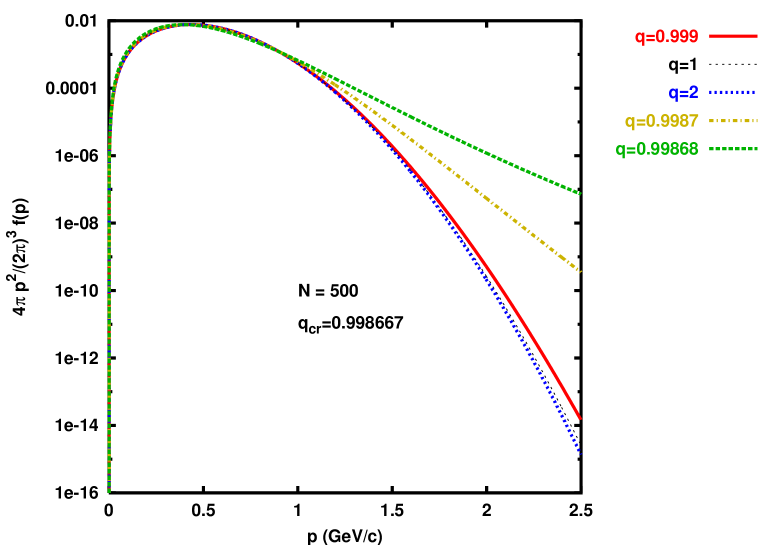
Figure 1: The one-particle distribution function for classical ideal gas of $N=500$ identical nucleons in extensive Rényi statistics at the temperature $T=100$ MeV for different values of $q$: $q=1$ (the second line from below) correspond to the Maxwell’s distribution function, other lines to the Rényi distribution function.

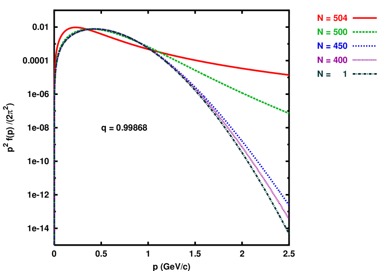
Figure 2: The one-particle distribution functions for classical ideal gas of $N=504,500,450,400$ and $1$ nucleons from the top down in extensive Rényi statistics at the temperature $T=100$ MeV and $q=0.99868$. The value of $N$ is restricted to $N<\frac{2}{3}\frac{q}{1-q\approx 504.38}$ at this choice of the Tsallis index.

Fig.1 shows the one-particle distribution function for different values of the entropic index $q$ in the above described classical ideal gas of Rényi statistics. The changes in behavior of the one-particle distribution function as the number of particles grow can be seen in Fig.2.

VII Conclusions

In conclusion we summarize the main idea of this paper. Two power-law tailed representations for non-Gibbs canonical distribution functions $p_{i}=p(E_{i})$ were obtained, the Wang and Rényi statistics. The equilibrium distribution function $p_{i}$ both for Wang and Rényi statistics satisfies the fundamental equation of thermodynamics. The transformation between them preserves the first and second laws of thermodynamics. The same is true for the Legendre transformation structure and for the thermodynamical relations for intensive quantities, like pressure and chemical potential in the microcanonical and in the canonical ensemble.

As a general rule the averages associated with Rényi statistics coincide with those for Wang statistics, but with a renormalized temperature and entropy. This makes the physical interpretation of these quantities more uncertain than it was in the Gibbs case. The physical temperature in Wang statistics reflects the transformation formula between Wang and Rényi statistics. The non-extensive entropy of Wang formalism changes, however, an important property of temperature, the satisfaction of the zeroth law of thermodynamics at dynamical and statistical independence request. The extensive Rényi statistics, on the contrary, passes even this test fulfilling all the requirements of equilibrium thermodynamics. The canonical distribution function also in this case is power-law tailed.

We have studied the Rényi statistics for classical ideal gas of massive nucleons with a finite number of particles. The equation of state (EOS) satisfies the ideal gas law ($pV=NkT$) familiar from Gibbs statistics in this case, but the distribution function differs from the Maxwell-Boltzmann one: it has a power-law tail. This difference may be seen experimentally only at large momenta in the tails of distributions, unless the Tsallis index is very near to the lower limit of $q_{cr}=1-2/(3N)$ for a classical ideal gas system consisting of $N$ particles.

Acknowledgments: This work has been supported by the Hungarian National Research Fund OTKA (T034269) and by the Hungarian-Russian Inter-Academy Collaboration, as well as partially supported by the Moldavian-U.S. Bilateral Grants Program, CRDF Projects MP2-3025 and MP2-3045. We acknowledge valuable remarks and fruitful discussions with V.D. Toneev and P. Lévai. One of authors, A.S.P, is grateful to the Department of Theoretical Physics of KFKI for the warm hospitality during his stay.

Appendix A Distribution function of canonical ensemble in incomplete statistics

Other definition for Lagrange function of canonical ensemble is

$$\Phi=\frac{S}{k}-\beta\left(\sum\limits_{i}p_{i}^{q}E_{i}-E\right).$$ (96)

After maximization of (96) we have

$$p_{i}^{q}=[q(1-(1-q)\beta E_{i})]^{\frac{q}{1-q}},$$ (97)

To normalize this distribution function it is necessary to introduce two new parameters instead of $\beta$

$$p_{i}^{q}=\frac{1}{Z}[1-(1-q)\beta^{\prime}E_{i}]^{\frac{q}{1-q}},$$ (98)

where the parameter $\beta^{\prime}\neq\beta$. Then the parameter $Z$ is founded from the norm eq. (2)

$$Z=\sum\limits_{i}\ [1-(1-q)\beta^{\prime}E_{i}]^{\frac{q}{1-q}}.$$ (99)

Let us to find the parameter $\beta^{\prime}$. Substituting (98) into eq. (1) we have

$$S=-k\ \frac{Z^{\frac{q-1}{q}}-1}{1-q}+k\beta^{\prime}Z^{\frac{q-1}{q}}\ E.$$ (100)

Differentiating eq. (100) on parameter $\beta^{\prime}$ and using eqs. (2), (3) we have

$$\frac{\partial S}{\partial\beta^{\prime}}=kZ^{\frac{q-1}{q}}\left[\frac{\partial\ln Z^{1/q}}{\partial\beta^{\prime}}(1-(1-q)\beta^{\prime}E)+\frac{\partial}{\partial\beta^{\prime}}(\beta^{\prime}E)\right].$$ (101)

On the other hand differentiating eq. (1) on $\beta^{\prime}$ and using distribution function (98) and eqs. (2), (3) we have

$$\frac{\partial S}{\partial\beta^{\prime}}=\frac{kZ^{\frac{q-1}{q}}}{1-q}\left[\frac{\partial\ln Z^{1/q}}{\partial\beta^{\prime}}(1-(1-q)\beta^{\prime}E)+E\right],$$ (102)

where was used $\partial E_{i}/\partial\beta^{\prime}=0$. Comparing eqs. (101) and (102) the following equality is valid

$$\frac{\partial S}{\partial\beta^{\prime}}=k\beta^{\prime}q^{-1}Z^{\frac{q-1}{q}}\ \frac{\partial E}{\partial\beta^{\prime}}.$$ (103)

Then the parameter $\beta^{\prime}$ is expressed from the temperature

$$\frac{1}{T}\equiv\frac{\partial S}{\partial E}=\frac{\partial S/\partial\beta^{\prime}}{\partial E/\partial\beta^{\prime}}=k\beta^{\prime}q^{-1}Z^{\frac{q-1}{q}}$$ (104)

and

$$\beta^{\prime}=\frac{qZ^{\frac{1-q}{q}}}{kT}.$$ (105)

In this respect it should be noted that in the paper of Q.A. Wang Wang00 multiplier $q$ from eq. (105) was lost as the entropy (100) was directly differentiated from $E$ without taking into account that the energy $E$ is not an independent variable of canonical ensemble $(T,V,N)$.

Substituting eq. (105) into eq. (100) and introducing the function $\Lambda$ in the following form (see Section II)

$$\Lambda\equiv kTq^{-1}\frac{Z^{\frac{q-1}{q}}-1}{1-q}=E-q^{-1}TS$$ (106)

for distribution function (98) and norm equation (99) we have

$$p_{i}^{q}=\left[1+(1-q)\frac{\Lambda-E_{i}}{kTq^{-1}}\right]^{\frac{q}{1-q}}$$ (107)

and

$$\sum\limits_{i}\left[1+(1-q)\frac{\Lambda-E_{i}}{kTq^{-1}}\right]^{\frac{q}{1-q}}=1.$$ (108)

Thus the minimization procedure of two different functionals (14) and (96) results in equivalency of distribution functions (18) and (107).

Appendix B The classical ideal gas in Wang’s representation

B.1 Case $q>1$

In the case $q>1$ it is convenient to use the following integral representation of the Euler’s Gamma function Prato ,

$$x^{-y} = \frac{1}{\Gamma(y)}\int\limits_{0}^{\infty}t^{y-1}e^{-tx}dt,\;\;\;\;\;\;\;\;\;Rex>0,Rey>0.$$ (109)

To solve eqs. (31), (32) one should substitute the values of $x=1+(1-q)q\beta\eta^{-1}(E-E_{i})$ and $y=q/(q-1)$ in the case of eq. (31) and the values of $x$ from the above and $y=1/(q-1)$ in the case of eq. (32) into formula (109). We get

$$\eta^{\frac{q}{1-q}}=\frac{1}{\Gamma(y)}\int\limits_{0}^{\infty}t^{y-1}\ e^{-t[1+(1-q)q\beta\eta^{-1}E]}\ Z_{1,N}(t(q-1)q\beta\eta^{-1})dt,$$ (110)

where $\beta=1/kT$ and $Z_{1,N}$ is the canonical partition function of the ideal Boltzmann gas of $N$ identical particles with the argument $\beta\rightarrow t(q-1)q\beta\eta^{-1}$

$$Z_{1,N}(t(q-1)q\beta\eta^{-1})=(t(q-1)q\eta^{-1})^{-\frac{3}{2}N}Z_{1,N}(\beta).$$ (111)

Taking into account (109) and (111), one can carry out the integration of integrand (110) with two values of $y$ from the eqs. (31), (32):

$$\eta^{-\frac{q}{1-q}-\frac{3}{2}N} = Z_{1,N}(\beta)\ \frac{\Gamma(\frac{q}{q-1}-\frac{3}{2}N)}{(q(q-1))^{\frac{3}{2}N}\Gamma(\frac{q}{q-1})}\ [1+(1-q)q\beta\eta^{-1}E]^{\frac{q}{1-q}+\frac{3}{2}N}$$ (112)

$$\eta^{-\frac{q}{1-q}-\frac{3}{2}N} = Z_{1,N}(\beta)\ \frac{\Gamma(\frac{1}{q-1}-\frac{3}{2}N)}{(q(q-1))^{\frac{3}{2}N}\Gamma(\frac{1}{q-1})}\ [1+(1-q)q\beta\eta^{-1}E]^{\frac{1}{1-q}+\frac{3}{2}N},$$ (113)

Solving the eqs. (112), (113) relative to the unknown variables $E$ and $\eta$, we have the following expressions

$$E = \frac{3}{2}N(q\beta)^{-1}\eta,$$ (114)

$$\eta = \left[1+(1-q)\frac{3}{2}N\right]^{-1}\ \left(Z_{1,N}(\beta)\frac{\Gamma(\frac{q}{q-1}-\frac{3}{2}N)}{(q(q-1))^{\frac{3}{2}N}\Gamma(\frac{q}{q-1})}\right)^{-\frac{1}{\frac{q}{1-q}+\frac{3}{2}N}},$$ (115)

which are valid under the conditions $-3N/2+q/(q-1)>0$ and $-3N/2+1/(q-1)>0$.

The one-particle distribution function are calculated from the eqs. (78), (80) by substituting the values of $x=1+(1-q)q\beta\eta^{-1}(E-\sum_{i=1}^{N}\vec{p}_{i}^{2}/2m)$ and $y=q/(q-1)$ into eq. (109)

$$f(\vec{p})=\frac{gV}{N(2\pi\hbar)^{3}}\frac{\eta^{\frac{q}{1-q}}}{\Gamma(\frac{q}{q-1})}\int\limits_{0}^{\infty}t^{\frac{q}{q-1}-1}\ e^{-t[1+(1-q)q\beta\eta^{-1}(E-\frac{\vec{p}^{2}}{2m})]}\ Z_{1,N-1}(t(q-1)q\beta\eta^{-1})dt.$$ (116)

Taking into account eqs. (109) and (111), we get for the integrant (116)

$$f(\vec{p}) = \left(\frac{\beta}{2\pi m}\right)^{3/2}\eta^{\frac{q}{1-q}+\frac{3}{2}(N-1)}Z_{1,N}(\beta)\ \frac{\Gamma(\frac{q}{q-1}-\frac{3}{2}(N-1))}{(q(q-1))^{\frac{3}{2}(N-1)}\Gamma(\frac{q}{q-1})}\times$$ (117)

$$\times\left[1+(1-q)q\beta\eta^{-1}(E-\frac{\vec{p}^{2}}{2m})\right]^{\frac{q}{1-q}+\frac{3}{2}(N-1)}.$$

Substituting the eqs. (114) and (115) into expression (117) we obtain the one-particle distribution function (81) with the coefficient (82) under restrictions described in the main text.

B.2 Case $q<1$

In the case $q<1$ should be used the Hankel’s contour integral in the complex plane Abram making the transformation $t\rightarrow tx$ with $x$ real and positive Prato ,

$$x^{y-1} = \Gamma(y)\frac{\imath}{2\pi}\oint\limits_{C}(-t)^{-y}e^{-tx}dt,\;\;\;\;\;\;\;\;\;Rex>0,|y|<\infty.$$ (118)

To solve eqs. (31), (32) one should substitute the values of $x=1+(1-q)q\beta\eta^{-1}(E-E_{i})$ and $y=1/(1-q)$ in the case of eq. (31) and the values of $x$ from the above and $y=(2-q)/(1-q)$ in the case of eq. (32) into formula (118). We get

$$\eta^{-\frac{q}{1-q}}=\Gamma(y)\frac{\imath}{2\pi}\oint\limits_{C}(-t)^{-y}e^{-t[1+(1-q)q\beta\eta^{-1}E]}\ Z_{1,N}(t(q-1)q\beta\eta^{-1})dt,$$ (119)

After calculations similar to eqs. (110)–(115) for the energy $E$ and the function $\eta$, we have

$$E = \frac{3}{2}N(q\beta)^{-1}\eta,$$ (120)

$$\eta = \left[1+(1-q)\frac{3}{2}N\right]^{-1}\ \left(Z_{1,N}(\beta)\frac{(q(1-q))^{-\frac{3}{2}N}\Gamma(\frac{1}{1-q})}{\Gamma(\frac{1}{1-q}+\frac{3}{2}N)}\right)^{-\frac{1}{\frac{q}{1-q}+\frac{3}{2}N}}.$$ (121)

The one-particle distribution function are calculated from the eqs. (78), (80) by substituting the values of $x=1+(1-q)q\beta\eta^{-1}(E-\sum_{i=1}^{N}\vec{p}_{i}^{2}/2m)$ and $y=1/(1-q)$ into eq. (118)

$$f(\vec{p})=\frac{gV}{N(2\pi\hbar)^{3}}\eta^{\frac{q}{1-q}}\Gamma(\frac{1}{1-q})\frac{\imath}{2\pi}\oint\limits_{C}(-t)^{-\frac{1}{1-q}}\ e^{-t[1+(1-q)q\beta\eta^{-1}(E-\frac{\vec{p}^{2}}{2m})]}\ Z_{1,N-1}(t(q-1)q\beta\eta^{-1})dt.$$ (122)

Taking into account eqs. (118) and (111), we get for the integrant (122)

$$f(\vec{p}) = \left(\frac{\beta}{2\pi m}\right)^{3/2}\eta^{\frac{q}{1-q}+\frac{3}{2}(N-1)}Z_{1,N}(\beta)\ \frac{(q(1-q))^{-\frac{3}{2}(N-1)}\Gamma(\frac{1}{1-q})}{\Gamma(\frac{1}{1-q}+\frac{3}{2}(N-1))}\times$$ (123)

$$\times\left[1+(1-q)q\beta\eta^{-1}(E-\frac{\vec{p}^{2}}{2m})\right]^{\frac{q}{1-q}+\frac{3}{2}(N-1)}.$$

Substituting the eqs. (120) and (121) into expression (123) we obtain the one-particle distribution function (81) with the coefficient (83).

References

• (1) J.W. Gibbs, Elementary principles in statistical mechanics, developed with especial reference to the rational foundation of thermodynamics, Yale Univ. Press, 1902.
• (2) R. Balescu, Equilibrium and nonequilibrium statistical mechanics, Wiley, New York, 1975.
• (3) C. Tsallis, Braz. J. Phys. 29 (1999) 1; cond-mat/9903356.
• (4) C. Tsallis, J. Stat. Phys. 52 (1988) 479; C. Tsallis, R.S. Mendes, A.R. Plastino, Physica A261 (1998) 534.
• (5) S. Abe, S. Martínez, F. Pennini, A. Plastino, Phys. Lett. A 281 (2001) 126.
• (6) Q.A. Wang, Euro. Phys. J. B 26 (2002) 357.
• (7) S. Abe, Phys. Rev. E 63 (2001) 061105.
• (8) Q.A. Wang and A. Le Méhauté, J. Math. Phys. 43 (2002) 5079.
• (9) S. Abe, Physica D 193 (2004) 218.
• (10) Q.A. Wang, Chaos, Solitons & Fractals, 12 (2001) 1431.
• (11) T. Jaynes in Statistical Physics ed. by W.K. Ford (Benjamin, NY, 1963).
• (12) D.H.E. Gross, Physica A 305 (2002) 99.
• (13) A. Rényi, Calcul de probabilité, Paris, Dunod, 1966; A. Wehrl, Rev. Mod. Phys. 50 (1978) 221.
• (14) E. Vives and A. Planes, Phys. Rev. Lett. 88 (2002) 020601.
• (15) D. Prato, Phys. Lett. A 203 (1995) 165.
• (16) K. Huang, Statistical Mechanics, Wiley, New York, 1963.
• (17) A.S. Parvan, V.D. Toneev and M. Płoszajczak, Nucl. Phys. A 676 (2000) 409.
• (18) A. Lavagno, Phys. Lett. A 301 (2002) 13.
• (19) M. Abramowitz, I.Stegun, Handbook of Mathematics Functions, Nat. Bur. Stand. Appl. Math. Ser., Vol.55, US GPO, Washington, DC, 1965.
Refer to caption