On the Efficiency of Topological Defect Formation
in the Systems of Various Size and (Quasi-) Dimensionality

Abstract

The experiments on verification of the Kibble–Zurek mechanism showed that topological defects are formed most efficiently in the systems of small size or low (quasi-)dimensionality, whereas in the macroscopic two- and three-dimensional samples a concentration of the defects, as a rule, is strongly suppressed. A reason for universality of such behavior can be revealed by considering a strongly-nonequilibrium symmetry-breaking phase transition in the simplest ${\varphi}^{4}$ field model. It is shown that the resulting distribution of the defects (domain walls) is formally reduced to the well-known Ising model, whose behavior changes dramatically in passing from a finite to infinite size of the system and from the low (D=1) to higher (D$\geq$2) dimensionality.

I Introduction

I.1 The concept of topological defects

Formation of topological defects by the strongly-nonequilibrium symmetry-breaking phase transitions is the subject of interest both in condensed matter and field theory. This is because of a close similarity between the Lagrangian of Landau–Ginzburg theory, widely used to describe phase transitions in the condensed-matter systems, and the Lagrangians of the modern elementary-particle theories (such as the standard electroweak model or various kinds of the Grand Unification Theories), which are substantially based on the concept of spontaneous symmetry breaking.

After the phase transitions in all the above-mentioned cases, the stable topological defects of the order parameter can arise, such as the monopoles, strings (vortices), and domain walls, depending on the symmetry group involved.

The most efficient mechanism of the defect formation is the so-called Kibble–Zurek scenario,Kibble (1976); Zurek (1985) which is based on the simple causality arguments. Namely, if during the phase transition the information about the order parameter can spread over the distance ${\xi}_{\text{eff}}$, then the phases of the order parameter should be established independently in the regions of characteristic size ${\xi}_{\text{eff}}$. As a result, after some relaxation following the phase transition, the stable defects of the order parameter should be formed at the typical separation ${\xi}_{\text{eff}}$ from each other. So, their concentration in a 3-dimensional system can be roughly estimated as

$$n\approx 1/\,{\xi}_{\text{eff}}^{\,d},$$ (1)

where $d=$ 3, 2, and 1 for the monopoles, strings (vortices), and domain walls, respectively; while the effective correlation length ${\xi}_{\text{eff}}$ depends on the particular system under consideration.

For example, in the symmetry breaking of Higgs fields by the cosmological phase transitions (i.e. a generation of mass of the elementary particles) ${\xi}_{\text{eff}}$ is commonly taken to beKlapdor-Kleingrothaus and Zuber (1997)

$${\xi}_{\text{eff}}\,\lesssim\,c\,/H_{\text{pt}}\,,$$ (2)

where $c$ is the speed of light, and $H_{\text{pt}}$ is Hubble constant at the instant of phase transition.

In the consideration of vortex generation by a superfluid phase transition in helium, the corresponding quantity is

$${\xi}_{\text{eff}}\,\approx\,c_{2}\,{\tau}_{\scriptscriptstyle Q}\,,$$ (3)

where $c_{2}$ is the speed of the second sound (i.e. a characteristic speed of propagation of information about the phase of the order parameter), and ${\tau}_{\scriptscriptstyle Q}$ is the so-called quench time (i.e. a characteristic time of the phase transition), defined as

$${\tau}_{\scriptscriptstyle Q}^{-1}=\,\left.\left(\frac{1}{T}\frac{dT}{dt}\right)\right|_{T=T_{c}}.$$ (4)

The similar definitions of ${\xi}_{\text{eff}}$ are used also for other systems (superconductors, liquid crystals, etc.).

I.2 Review of experimental data

Although Kibble–Zurek scenario was proposed initially in the context of cosmological phase transitions in the field theories admitting the symmetry breaking (in fact, the first idea of such kind was put forward by BogoliubovBogoliubov (1966) almost 40 years ago), much efforts have been undertaken in the last decade to verify this phenomenon by the laboratory experiments. These works were originated by Chuang, et al.Chuang et al. (1991) in 1991, and about a dozen of such experiments were performed by now in various superfluid and superconducting systems. They are summarized in Table 1. (This table does not show a number of experiments with liquid crystals, aimed at the detailed study of inner structure of the defects without measuring the rates of their formation.)

Table 1: Summary of experiments on the defect formation by strongly-nonequilibrium symmetry-breaking phase transitions. A positive result ($+$) implies an agreement with the Kibble–Zurek estimate within a factor about unity; and the negative result ($-$), a disagreement by a few times to a few orders of magnitude.

			Initiation	Method	(Quasi-)	Size	Result
Experimental object			of phase	of	dimen-	of	of expe-	Refs.
			transition	detection	sionality	sample	riment
Superfluids		4He	Expansion	Second sound	3	macro	–	Hendry et al., 1994; Dodd et al., 1998
			of sample	absorption
		3He	Neutron	Calorimetry	3	micro	+	Bäuerle et al.,1996
			irradiation
				Nuclear magne-	3	micro	+	Ruutu et al.,1996
				tic resonance
Super-	Thin films		Heating–	SQUID	2	macro	–	Carmi and Polturak,1999; Maniv et al.,2003
conduc-			cooling
tors			cycles	SQUID micro-	2	macro	–	Kirtley et al.,2003
				scope
	Multi-Josephson-			SQUID	1	macro	+	Carmi et al.,2000
	junction loop
	Annular Josephson			Voltage mea-	1	macro	+	Monaco et al.,2002
	tunnel junctions			surement

Analysis of the table reveals a quite interesting tendency: the topological defects are formed most efficiently in the systems of small size or low (quasi-) dimensionality, for example, the one-dimensional multi-Josephson-junction loops (MJJL) Carmi et al. (2000) and annular Josephson tunnel junctions Monaco et al. (2002) as well as in microscopic hot bubbles of ³He produced by neutron irradiation. Bäuerle et al. (1996); Ruutu et al. (1996) On the other hand, the concentration of the defects in macroscopic systems of higher dimensionality, e.g. the two-dimensional superconductor films Carmi and Polturak (1999); Maniv et al. (2003); Kirtley et al. (2003) and three-dimensional volume samples of ⁴He (Refs. Hendry et al., 1994; Dodd et al., 1998), was found to be considerably less than the theoretical predictions.

In principle, there may be various explanations of the above fact (for example, different material parameters of the substances listed in Table 1). The aim of the present work is to propose another explanation, which is based on the universal geometric properties of the systems under consideration, namely, their size and dimensionality (or quasi-dimensionality).

II The model of defect formation

II.1 Initial assumptions and equations

To carry out all calculations in analytic form, let us consider the simplest ${\varphi}^{4}$-model of real scalar field (the order parameter), whose Lagrangian

$${\cal L}\,({\bf r},t)\,=\,\frac{1}{2}\,\big{[}{\left({\partial}_{t}\varphi\right)}^{2}\!-\,{\left(\nabla\varphi\right)}^{2}\big{]}\,-\>\frac{\lambda}{4}\,{\big{[}\,{\varphi}^{2}\!-\left({\mu}^{2}/\lambda\right)\big{]}}^{2}$$ (5)

admits the discrete ($\mathbb{Z}_{2}$) symmetry breaking.

Two stable vacuum states of this field (which, for the sake of convenience, will be marked by the oppositely directed arrows) are

$${\varphi}_{\uparrow\downarrow}=\pm\,{\varphi}_{0}=\,\pm\,\mu\,/\sqrt{\lambda}\;;$$ (6)

the structure of a domain wall between them, located at $x=x_{0}$, is described as

$$\varphi\,(x)=\,\pm\,{\varphi}_{0}\tanh\big{[}\frac{\mu}{\sqrt{2}}\,(x-x_{0})\big{]}\,;$$ (7)

and the specific energy concentrated in this wall equals

$$E=\,\frac{2\,\sqrt{2}}{3}\,\frac{{\mu}^{3}}{\lambda}\;.$$ (8)

Let a domain structure formed after a strongly-nonequilibrium phase transition in this model be approximated by a regular rectangular grid with a cell size about the effective correlation length ${\xi}_{\text{eff}}$, whose definition in the Kibble–Zurek scenario was already discussed above in Sec. I.1. The particular value of ${\xi}_{\text{eff}}$ is not of importance here, but we shall assume that it is sufficiently large in comparison with a characteristic thickness of the domain wall $\sim\!1/\mu$. As a result, the final pattern of vacuum states (6) after the phase transition will look like a distribution of spins on the rectangular grid.

The key assumption of the Kibble–Zurek mechanism is that the final symmetry-broken states of the field $\varphi$ in two neighboring cells are completely independent of each other. Then, the probability of formation of a domain wall between them is given evidently by the ratio of the number of statistical configurations involving the domain wall to the total number of configurations:

$$P_{\rm\scriptscriptstyle KZ}=2/4=1/2\;;$$ (9)

and the resulting concentration of the defects (domain walls) will be

$$n_{\rm\scriptscriptstyle KZ}=\frac{1}{2}\>\frac{\text{D}}{{\xi}_{\text{eff}}^{\text{D}}}\;,$$ (10)

where D is the effective dimensionality of the system.

In fact, such approach is not sufficiently accurate, because a nonzero value of the order parameter formed after the phase transition represents a coherent state of Bose condensate, in which the specific quantum correlations may occur even at the distances exceeding the effective correlation length ${\xi}_{\text{eff}}$ derived from the “classical” arguments. This kind of correlations was clearly demonstrated by the MJJL experiment Carmi et al. (2000).

II.2 Overview of MJJL experiment

For the sake of completeness, let us briefly remind the basic idea and result of the multi-Josephson-junction loop experiment by Carmi, et al., Carmi et al. (2000) whose sketch is presented in Fig. 1.

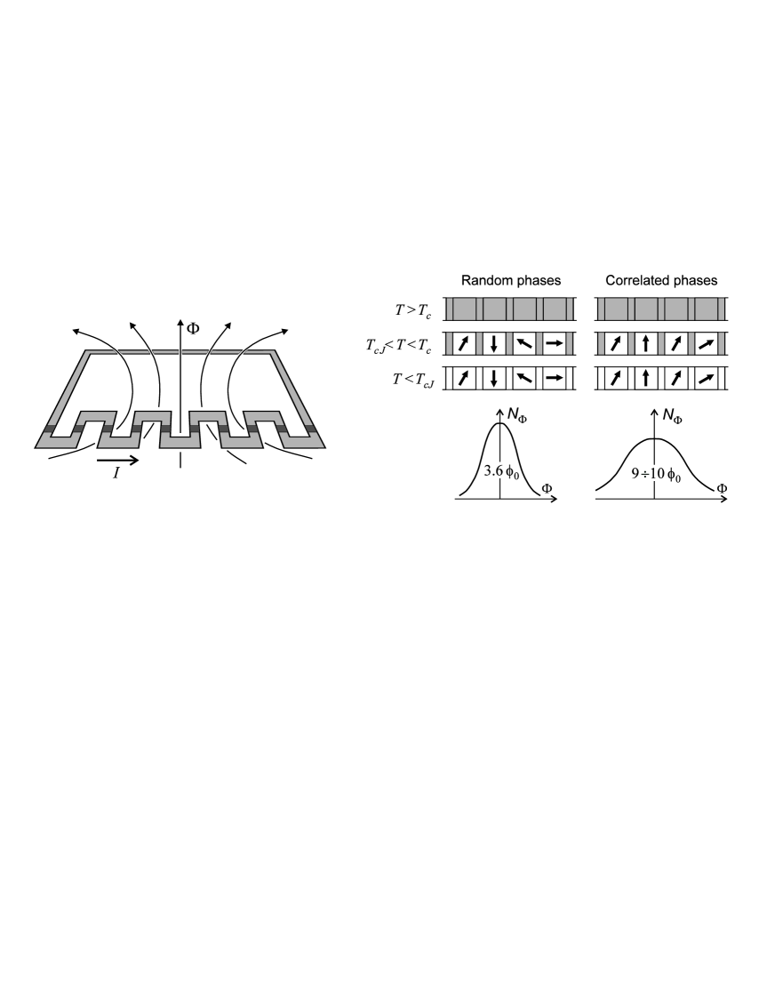
Figure 1: Sketch of the experimental setup (left) and basic results (right) of MJJL experiment.

A thin quasi-one-dimensional winding strip was engraved at the boundary between two crystalline grains of YBa₂Cu₃O${}_{7\mbox{-}\delta}$ high-temperature superconductor film, thereby forming a loop of 214 superconductor segments separated by the grain-boundary Josephson junctions. This system experienced multiple heating–cooling cycles in the temperature range 77 K to $\sim$100 K, which covers both the critical temperature of superconducting phase transition in the segments of the loop ($T_{c}=90$ K) and in the junctions between them ($T_{cJ}=83\div 85$ K).

There is evidently no order parameter in the entire loop as long as $T>T_{c}$. Next, when the temperature drops below $T_{c}$ but remains above $T_{cJ}$ (i.e. $T_{cJ}<T<T_{c}$), some value of the order parameter should be established in each segment, as is schematically shown by arrows in the right-hand part of Fig. 1. Since these segments are separated by nonconducting Josephson junctions, it seems to be reasonable to assume that the phase jumps between them are random (i.e. uncorrelated to each other). Finally, when the temperature drops below $T_{cJ}$, the entire loop becomes superconducting and, due to the above-mentioned jumps, a phase integral along the loop, in general, should be nonzero. As a result, the electric current $I$, circulating along the loop, and the corresponding magnetic flux $\Phi$, penetrating the loop, will be spontaneously generated.

So, if the phase jumps in the intermediate state $T_{cJ}<T<T_{c}$ were absolutely uncorrelated, then distribution of the spontaneously-trapped magnetic flux in the particular experimental setup Carmi et al. (2000) would be given by the normal (Gaussian) law with a characteristic width $3.6\,{\phi}_{0}$ (where ${\phi}_{0}$ is the magnetic-flux quantum). On the other hand, the actual experimental distribution was found to be over two times wider; and this anomaly was satisfactorily interpreted by the authors of the experiment assuming that the phase jumps in the intermediate state were not random but correlated to each other so that the probability $P({\delta}_{i})$ of the phase difference ${\delta}_{i}$ in the $i$’th junction was

$$P({\delta}_{i})\sim\exp[-{E_{J}}({\delta}_{i})\,/\,T_{c}]\>,$$ (11)

where $E_{J}$ is the energy concentrated in the Josephson junction, and $T_{c}$ is the phase transition temperature, measured in energy units.

The nature of the above-mentioned correlations between the phases of order parameter in the spatially-separated regions is not sufficiently understood yet. They may be one of manifestations of the specific quantum “entanglement”, revealed by now in various quantum systems. We are not going to discuss here this problem in more detail but assume that the correlations like (11) are typical for all Bose condensates formed by the symmetry-breaking phase transitions. As will be seen from the subsequent analysis, such an assumption will enable us to interpret satisfactorily a wide range of experimental data on the efficiency of formation of topological defects. Just this fact can be considered as indirect confirmation of universality of (11).

II.3 Improvement of the standard estimates

As follows from the above discussion, the probabilities of various field configurations after a symmetry-breaking phase transition should be calculated taking into account the energy concentrated in the defects. As a result, a pattern of the domains formed by the strongly-nonequilibrium phase transition in the ${\varphi}^{4}$ lattice model will look like a distribution of spins in Ising model at the temperature $T$ which is formally equivalent to the critical temperature $T_{c}$ of the initial ${\varphi}^{4}$-model. All aspects of this formal correspondence are summarized in Table 2.

Table 2: Formal correspondence between the phase transitions in ${\varphi}^{4}$ and Ising models.

	$\bm{{\varphi}^{4}}$-model	Ising model
1.	State formed after a	Thermodynamically-
	strongly-nonequilibrium	equilibrium state.
	phase transition.
2.	Elementary domains of	Spins.
	the symmetry-broken state.
3.	Statistical sum $Z$ for	Thermodynamical statistical
	distribution of the domains	sum $Z$ for spin distribution.
	with various vacuum states.
4.	Critical temperatures $T_{c}$	Temperature $T$ varying in
	for various systems.	the course of the phase
		transition.
5.	Suppression of the domain	Phase transition in the spin
	wall formation.	system.

Then, the probability of formation of a domain wall should be calculated as

$$P=\frac{\hphantom{1}T_{c}^{2}}{E\,\text{D}N^{\text{D}}}\;\frac{\partial}{\partial T_{c}}\ln Z^{(\text{D})}\>,$$ (12)

where $E$ is the energy of the elementary domain wall (i.e. at one boundary between two neighboring cells), $N$ is the number of cells along each side of the lattice, and

$$Z^{(\text{D})}=\sum_{i}\exp(-{\varepsilon}_{i}\,/\,T_{c})$$ (13)

is the usual statistical sum over all possible spin configurations of the Ising model, where ${\varepsilon}_{i}$ is the total energy of $i$’th configuration.

Particularly, for 1-dimensional system with periodic boundary conditions,

$$Z^{(1)}\,=\,\sum_{i=1}^{\scriptstyle N}\sum_{s_{i}=\pm 1}\exp\left\{\vphantom{\frac{A}{A}}\right.\!-\frac{E}{T_{c}}\,\sum_{k=1}^{\scriptstyle N}\,\frac{1}{2}\,(1-s_{k}s_{k+1})\left.\vphantom{\frac{A}{A}}\right\};$$ (14)

for 2-dimensional system,

$$Z^{(2)}\,=\,\sum_{i=1}^{\scriptstyle N}\sum_{j=1}^{\scriptstyle N}\sum_{s_{ij}=\pm 1}\exp\left\{\vphantom{\frac{A}{A}}\right.\!-\frac{E}{T_{c}}\,\sum_{k=1}^{\scriptstyle N}\,\sum_{l=1}^{\scriptstyle N}\,\frac{1}{2}\,(\,2-$$

$$s_{kl}s_{k+1,l}\,-\,s_{kl}s_{k,l+1})\left.\vphantom{\frac{A}{A}}\right\};$$ (15)

and so on. Here, $s_{k}$ and $s_{kl}$ are the spin-like variables describing the broken-symmetry states in the $k$’th and $(kl)$’th cell, respectively.

As is known (e.g. Ref. Rumer and Ryvkin, 1980), the Ising model for one-dimensional as well as the finite-size higher-dimensional systems does not experience a phase transition to the ordered state at any value of the ratio $E/T$. From the viewpoint of the domain wall formation by the strongly-nonequilibrium phase transition in ${\varphi}^{4}$-model (Table 2), this means that concentration of the defects will not differ considerably from the standard Kibble–Zurek estimate, because the probability of defect formation $P$ at the scale of the effective correlation length ${\xi}_{\text{eff}}$ will not deviate substantially from $P_{\rm\scriptscriptstyle KZ}=1/2\sim 1$.

On the other hand, the Ising model for the sufficiently large (infinite-size) two- and three-dimensional systems does experience a phase transition to the ordered state at some value of $E/T\!\sim\!1$. As a result, the concentration of domain walls in the corresponding ${\varphi}^{4}$-model at large ratios $E/T_{c}$ should be suppressed dramatically, due to formation of macroscopic regions with the same value of the order parameter, covering a great number of cells of the effective correlation length ${\xi}_{\text{eff}}$. (To avoid misunderstanding, let us emphasize once again that the different values of $T_{c}$ should be understood here as the critical temperatures for various physical systems described by the ${\varphi}^{4}$-model, and they formally correspond to the variable temperature $T$ of a fixed Ising system.)

II.4 Particular example

The general conclusions formulated above can be illustrated by the particular example in Fig. 2, which represents the concentration of domain walls $n$ normalized to the standard Kibble–Zurek value $n_{\rm\scriptscriptstyle KZ}$ as function of $E/T_{c}$ for the following three systems:
(1) one-dimensional Ising model, which admits the exact solution (see, for example, Ref. Isihara, 1971 for more details);
(2) two-dimensional $6{\times}6$-cell Ising model with periodic boundary conditions, which simulates quite well the system of infinite size; and
(3) two-dimensional $6{\times}6$-cell Ising model with free boundaries (where no energy is concentrated), which is an example of a microscopic system.
(The particular size of 6 cells along each side of the lattice was taken quite arbitrarily, just as the value at which a numerical computation of the statistical sum (15) is not too cumbersome; details of the calculations can be found in Appendix.)

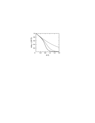
Figure 2: Concentration of the defects $n$ normalized to the standard Kibble–Zurek value $n_{\rm\scriptscriptstyle KZ}$ as function of the ratio of the domain wall energy $E$ to the phase transition temperature $T_{c}$ for the infinite-size 1D Ising model (dashed curve), $6{\times}6$-cell 2D Ising model with periodic boundary conditions (solid curve), and the same model with free boundaries (dotted curve).

As is seen in Fig. 2, at $E/T_{c}\approx 1$ the concentration of defects in one-dimensional system (dashed curve) differs from the standard Kibble–Zurek value by less than two times; in microscopic two-dimensional system (dotted curve), by three times; while in the macroscopic two-dimensional system (solid curve) it is suppressed by an order of magnitude. Such suppression becomes much stronger when the ratio $E/T_{c}$ increases: for example, at $E/T_{c}\approx 2$ the difference between each of the curves is over an order of magnitude.

III Discussion

As follows from the above consideration, the specific thermal correlations between the phases of Bose condensates in separated spatial regions, revealed for the first time in MJJL experiment, can show us a general way for explanation of the entire diversity of experimental data on the topological defect formation. Unfortunately, the results of our simplified model cannot be confronted quantitatively with the ones cited in Table 1, because the superfluids and superconductors possess more complex order parameters and Lagrangians than (5). So, more elaborate calculations are required.

Next, it is important to emphasize that the refined concentration of defects

$$n=f(E/T_{c})\>n_{\rm\scriptscriptstyle KZ}({\xi}_{\text{eff}}({\tau}_{\scriptscriptstyle Q}))$$ (16)

possesses exactly the same dependence on the quench rate ${\tau}_{\scriptscriptstyle Q}$ as in the classical Kibble–Zurek scenario. So, this dependence, often measured in the experiments, in general, cannot serve for discrimination between the models; the absolute values of the defect concentration are always necessary.

Finally, let us mention that the ideas described in the present work can be applied also to solving the problem of excessive concentration of topological defects predicted after the cosmological phase transitions of Higgs fields.Dumin (2003)

*

Appendix A Computation of the statistical sums

For the sake of completeness, let us present the formulas used for drawing the curves in Fig. 2.

Table 3: Nonzero statistical weight factors for $6{\times}6$-cell Ising model with periodic boundary conditions.

$k$	$C^{\text{per}}_{k}$ and $C^{\text{per}}_{72-k}$	$k$	$C^{\text{per}}_{k}$ and $C^{\text{per}}_{72-k}$
0	2	20	17 569 080
4	72	22	71 789 328
6	144	24	260 434 986
8	1 620	26	808 871 328
10	6 048	28	2 122 173 684
12	35 148	30	4 616 013 408
14	159 840	32	8 196 905 106
16	804 078	34	11 674 988 208
18	3 846 576	36	13 172 279 424

Table 4: Nonzero statistical weight factors for $6{\times}6$-cell Ising model with free boundaries.

$k$	$C^{\text{free}}_{k}$ and $C^{\text{free}}_{60-k}$	$k$	$C^{\text{free}}_{k}$ and $C^{\text{free}}_{60-k}$
0	2	16	15 444 302
2	8	17	33 435 520
3	48	18	69 487 240
4	100	19	138 380 976
5	288	20	263 185 168
6	1 132	21	476 852 512
7	3 168	22	821 190 292
8	8 824	23	1 340 056 928
9	25 744	24	2 065 952 532
10	71 064	25	3 000 507 536
11	186 624	26	4 093 604 824
12	484 210	27	5 230 849 920
13	1 214 336	28	6 244 335 166
14	2 931 560	29	6 951 501 824
15	6 853 760	30	7 206 345 520

As is known, all characteristics of the one-dimensional Ising model can be calculated analytically (for a detailed description of the method see, for example, Ref. Isihara, 1971). The resulting formula for a defect concentration in a chain of length $N$ with periodic boundary conditions is

$$n/n_{\rm\scriptscriptstyle KZ}=\>2\,\exp(-E/T_{c})\times\vphantom{\frac{X}{X}}$$ (17)

$$\frac{(1+\exp(-E/T_{c}))^{N-1}-(1-\exp(-E/T_{c}))^{N-1}}{(1+\exp(-E/T_{c}))^{N}+(1-\exp(-E/T_{c}))^{N}}\;,$$

which in the case of infinite chain is reduced to

$$n/n_{\rm\scriptscriptstyle KZ}=\frac{2\,\exp(-E/T_{c})}{1+\exp(-E/T_{c})}\;.$$ (18)

For the two-dimensional infinite lattice, statistical sum (13) can be reduced by the well-known technique to some integral over two variables, and the asymptotics of this integral can be obtained analytically just in the point of the phase transition of Ising model (for more details see, for example, Ref. Landau and Lifshitz, 1969). Unfortunately, these results are of little value for our work, since we need to know the statistical sum in a wide range of temperature. Besides, this method cannot be applied to the finite-size lattices, which are also of considerable interest for us.

So, we used a more straightforward approach. In general, the statistical sum (13) can be rewritten as

$$Z^{(\text{D})}=\sum_{k}C_{k}\exp(-kE/\,T_{c})\;,$$ (19)

where $C_{k}$ is the statistical weight of configurations involving $k$ elementary domain walls with energy $E$ each. In the particular case of two-dimensional $6{\times}6$-cell Ising model, the coefficients $C_{k}$ were calculated by the methods of computer algebra both for the lattice with periodic boundary conditions (in which every domain wall carries the energy $E$) and with the free boundaries (where only the inner domain walls contribute to the total energy of the configuration). The corresponding coefficients $C^{\text{per}}_{k}$ and $C^{\text{free}}_{k}$ are listed in Tables 3 and 4.

Next, the concentration of domain walls is obtained by substituting (19) into (12); and the final result takes the form

$$n/n_{\rm\scriptscriptstyle KZ}=\>\frac{2\;\displaystyle{\sum}_{k}k\,C_{k}\exp(-kE/T_{c})}{\displaystyle\text{D}N^{\text{D}}\>{\sum}_{k}C_{k}\exp(-kE/T_{c})}\;,$$ (20)

where in the case under consideration $\text{D}\!=2$ and $N\!=6$.

References

- Kibble (1976) T. Kibble, J. Phys. A 9, 1387 (1976).
- Zurek (1985) W. Zurek, Nature (London) 317, 505 (1985).
- Klapdor-Kleingrothaus and Zuber (1997) H. Klapdor-Kleingrothaus and K. Zuber, Particle Astrophysics (Inst. Phys. Publ., Bristol, 1997).
- Bogoliubov (1966) N. Bogoliubov, Suppl. Nuovo Cimento (Ser. prima) 4, 346 (1966).
- Chuang et al. (1991) I. Chuang, R. Durrer, N. Turok, and B. Yurke, Science 251, 1336 (1991).
- Hendry et al. (1994) P. Hendry, N. Lawson, R. Lee, P. McClintock, and C. Williams, Nature (London) 368, 315 (1994).
- Dodd et al. (1998) M. Dodd, P. Hendry, N. Lawson, P. McClintock, and C. Williams, Phys. Rev. Lett. 81, 3703 (1998).
- Bäuerle et al. (1996) C. Bäuerle, Y. Bunkov, S. Fisher, H. Godfrin, and G. Pickett, Nature (London) 382, 332 (1996).
- Ruutu et al. (1996) V. Ruutu, V. Eltsov, A. Gill, T. Kibble, M. Krusius, Y. Makhlin, B. Plaçais, G. Volovik, and Wen Xu, Nature (London) 382, 334 (1996).
- Carmi and Polturak (1999) R. Carmi and E. Polturak, Phys. Rev. B 60, 7595 (1999).
- Maniv et al. (2003) A. Maniv, E. Polturak, and G. Koren, Phys. Rev. Lett. 91, 197001 (2003).
- Kirtley et al. (2003) J. Kirtley, C. Tsuei, and F. Tafuri, Phys. Rev. Lett. 90, 257001 (2003).
- Carmi et al. (2000) R. Carmi, E. Polturak, and G. Koren, Phys. Rev. Lett. 84, 4966 (2000).
- Monaco et al. (2002) R. Monaco, J. Mygind, and R. Rivers, Phys. Rev. Lett. 89, 080603 (2002).
- Rumer and Ryvkin (1980) Y. Rumer and M. Ryvkin, Thermodynamics, Statistical Physics, and Kinetics (Mir, Moscow, 1980).
- Isihara (1971) A. Isihara, Statistical Physics (Academic Press, NY, 1971).
- Dumin (2003) Y. Dumin, in Frontiers of Particle Physics (World Scientific Co, Singapore, 2003), p. 289, eprint hep-ph/0204154.
- Landau and Lifshitz (1969) L. Landau and E. Lifshitz, Statistical Physics (Pergamon Press, Oxford, 1969).