Effective Lagrangian approach to Higgs-mediated FCNC top quark decays

Abstract

The flavor changing neutral current (FCNC) transitions $t\to q^{\prime}H$ and $t\to q^{\prime}V_{i}$ $(V_{i}=\gamma,g,Z)$ are studied in the context of the effective Lagrangian approach. We focus on the scenario in which these decays are predominantly induced by new physics effects arising from the Yukawa sector extended with dimension-six $SU_{L}(2)\times U_{Y}(1)$-invariant operators, which generate the most general CP-even and CP-odd $tq^{\prime}H$ vertex at the tree level. For the unknown coefficients, we assume a slightly modified version of the Cheng-Sher ansatz. We found that the branching ratio for the Higgs-mediated FCNC $t\to q^{\prime}V_{i}$ decays are enhanced by two or three orders of magnitude with respect to the results expected in models with extended Higgs sectors, such as the general two-Higgs doublet model. We discuss the possibilities of detecting this class of decays at the LHC.

I Introduction

The fact that the top quark is the only known fermion whose mass is comparable to the electroweak symmetry breaking scale suggests that it may be more sensitive to new physics effects than the remaining known fermions. Furthermore, the new dynamic effects are likely to be more evident in those top quark processes that are forbidden or strongly suppressed in the standard model (SM). Therefore, the study of the flavor changing neutral current (FCNC) transitions of the top quark could be the clue to detect new physics effects Review . In the SM, the $t\to c\gamma$, $t\to cZ$, and $t\to cH$ decays have branching ratios of the order of $10^{-13}$ Perez ; MP , which are too small to be detected at collider experiments. Any signal of such transitions will thus represent a neat evidence of new physics. So far, most studies on FCNC top quark transitions have focused on the $t\to cV_{i}$ decays, with $V_{i}=\gamma,Z,g$. However, since the Higgs boson $H$ may be as heavy as the top quark, the electroweak symmetry would also be maximally broken by this particle, thereby opening the possibility that some Higgs-mediated FCNC effects could be observed in future experiments. The study of this scenario is encouraged by the possibility of a common source responsible for both symmetry breaking and flavor changing effects, along with the experimental prospects: a copious production of top quark events is expected at the CERN large hadron collider (LHC).

Although scalar-mediated FCNC effects are strongly suppressed in the SM, they may be more significant in some of its extensions. For instance, the general two-Higgs doublet model (THDM-III) has the simplest extended Higgs sector that naturally introduces scalar-mediated FCNC effects at the tree level ORIGINAL ; SAVAGE . As a result, in that model the scalar-mediated top quark transitions may have branching ratios several orders of magnitude larger that those predicted by the SM REINA1 ; REINA2 ; THDMH ; DPTT . A similar conclusion was reached in the case of Higgs-mediated lepton-flavor violating processes THDML ; DT . Large Higgs-mediated FCNC effects can also be naturally induced in other SM extensions, such as the minimal supersymmetric standard model SUSYH .

As already mentioned, FCNC effects can be induced in theories with an extended scalar sector or a larger gauge group ORIGINAL ; THDMH ; THDML . In the present work we are interested in those new physics effects that induce FCNC top quark transitions predominantly mediated by the SM Higgs boson. We will take a similar approach to that used in Ref. DT to study Higgs boson-mediated lepton flavor violating effects. We found it convenient to perform a model independent study by means of the effective Lagrangian approach (ELA), which is appropriate to investigate new physics effects in processes that are forbidden or strongly suppressed in the SM Buchmuller ; EW . In this scheme no new degrees of freedom are introduced but the SM ones. We will assume an effective Lagrangian composed of only one Higgs doublet, which will be taken as the one responsible for FCNCs, which in turn may arise from virtual effects of heavy particles lying beyond the Fermi scale. Moreover, motivated by the role played by the Yukawa sector in flavor physics, we will assume that the main source of Higgs-mediated FCNC top quark transitions is the Yukawa sector extended with dimension-six operators. We would like to emphasize that the scenario that we are interested in is different to that arising in models with extended scalar sectors SAVAGE ; REINA2 , in which the scalar FCNCs are induced at the tree level by the presence of additional Higgs multiplets rather than by virtual heavy particles.

In the scenario already described, the $tq^{\prime}V_{i}$ vertices ($q^{\prime}=u,c$) would be necessarily induced at the one-loop level via the anomalous $tq^{\prime}H$ coupling. In fact, all of the $tq^{\prime}V_{i}$ couplings but the $tq^{\prime}Z$ one can only arise at the one-loop level in any renormalizable theory. They can be conveniently parametrized through the following effective Lagrangian HanVertices

$$\mathcal{L} = \bar{t}\Bigg{\{}\frac{ie}{2m_{t}}\,(\kappa_{tq^{\prime}\gamma}+i\widetilde{\kappa}_{tq^{\prime}\gamma}\gamma_{5})\sigma_{\mu\nu}\,F^{\mu\nu}+\frac{ig_{s}}{2m_{t}}\,(\kappa_{tq^{\prime}g}+i\widetilde{\kappa}_{tq^{\prime}g})\sigma_{\mu\nu}\frac{\lambda^{a}}{2}\,G^{\mu\nu}_{a}+$$ (1)

$$\frac{g}{2c_{W}}\Big{[}\gamma_{\mu}(v_{tq^{\prime}Z}+a_{tq^{\prime}Z}\gamma_{5})Z^{\mu}+\frac{i}{2m_{t}}(\kappa_{tq^{\prime}Z}+i\widetilde{\kappa}_{tq^{\prime}Z}\gamma_{5})\sigma_{\mu\nu}Z^{\mu\nu}\Big{]}\Bigg{\}}q^{\prime}+{\rm H.c.}$$

The main goal of this work is to assess the impact of the $tq^{\prime}H$ vertex on the $tq^{\prime}V_{i}$ vertices and thus on the rare $t\to q^{\prime}V_{i}$ decays. Since the effective Yukawa sector can generate the most general $tq^{\prime}H$ coupling, it would induce both the CP-even and CP-odd $tq^{\prime}V_{i}$ couplings at the one-loop level. We believe that this is an interesting scenario as it is expected that the Higgs-top dynamics is sensitive to new physics effects. In particular, FCNC effects would be favored by the involved mass scales: we will show below that even though the $t\to q^{\prime}V_{i}$ decays are induced at the one-loop level by the $tq^{\prime}H$ vertex, the corresponding amplitudes are unsuppressed because both the external and the internal scales, $m_{t}$ and $m_{H}$, are expected to be of the same order of magnitude. The most general $tq^{\prime}H$ vertex involves two unknown parameters: a CP-even one, $\epsilon_{tq^{\prime}H}$, and a CP-odd one, $\widetilde{\epsilon}_{tqH}$, whose order of magnitude can be constrained from low-energy data. Since the bounds on these parameters turn out to be somewhat loose, we will adopt a slightly modified version of the Cheng-Sher ansatz to estimate them and predict the rates of the FCNC top quark decays.

The rest of this paper has been organized as follows. In Sec. II we will derive the $tq^{\prime}H$ vertex from the most general effective Yukawa-type operators of dimension six, which simultaneously incorporate both FCNC and CP-violating effects. Section III is devoted to the calculation of the $tq^{\prime}H$ contribution to the $tq^{\prime}V_{i}$ couplings. In Sec. IV, we evaluate the rates of the FCNC top quark decays and discuss the results. Particular attention will be paid to emphasize the differences between the scenario discussed in this work and some specific models. Finally, the conclusions are presented in Sec. V.

II Effective Yukawa sector and Higg-mediated FCNC effects

It is well-known that the SM Yukawa sector is both flavor- and CP-conserving. FCNC effects can arise at tree level in any renormalizable Yukawa sector if more scalar fields are incorporated. However, it is not necessary to introduce new degrees of freedom to generate both FCNC and CP-violating effects if Dyson power counting criterion of renormalizability is not granted as a fundamental principle when constructing the Lagrangian. Indeed, it is only necessary to extend the Yukawa sector with dimension-six operators to induce the most general couplings of the Higgs boson to the quarks. A Yukawa sector with those features, which respects the $SU_{L}(2)\times U_{Y}(1)$ symmetry, has the following structure Shalom

$$\mathcal{L}^{Y}_{eff}=-Y^{d}_{ij}(\bar{Q}_{i}\Phi d_{j})-Y^{u}_{ij}(\bar{Q}_{i}\widetilde{\Phi}u_{j})-\frac{\alpha^{d}_{ij}}{\Lambda^{2}}(\Phi^{\dagger}\Phi)(\bar{Q}_{i}\Phi d_{j})-\frac{\alpha^{u}_{ij}}{\Lambda^{2}}(\Phi^{\dagger}\Phi)(\bar{Q}_{i}\widetilde{\Phi}u_{j})+{\rm H.c.},$$ (2)

where $Y_{ij}$, $Q_{i}$, $\Phi$, $d_{i}$, and $u_{i}$ stand for the usual Yukawa constants, the left-handed quark doublet, the Higgs doublet, and the right-handed quark singlets of down and up type, respectively. The $\alpha_{ij}$ constants, which parametrize the details of the underlying physics, could be determined once the fundamental theory is known. Since the dimension-six operators can be generated at the tree level in the fundamental theory EW , they would not be suppressed by the loop factors as it occurs with those operators that generate the gluon- and photon-mediated FCNC top quark transitions at the tree level HanVertices ; FHTT .

After spontaneous symmetry breaking, $\mathcal{L}^{Y}_{eff}$ can be diagonalized as usual via the unitary matrices $V^{u,d}_{L}$ and $V^{u,d}_{R}$, which relate gauge states to mass eigenstates. The diagonalized Lagrangian can be written in the unitary gauge as follows:

$$\mathcal{L}^{Y}_{eff} = -\left(1+\frac{gH}{2m_{W}}\right)\left(\bar{D}M^{d}D+\bar{U}M^{u}U\right)-H\left[1+\frac{gH}{4m_{W}}\left(3+\frac{gH}{2m_{W}}\right)\right]$$ (3)

$$\times\Big{[}\bar{D}(\Omega^{d}P_{R}+\Omega^{d{\dagger}}P_{L})D+\bar{U}(\Omega^{u}P_{R}+\Omega^{u{\dagger}}P_{L})U\Big{]},$$

where $M^{d,u}$ are diagonal mass matrices, whereas $U^{T}=(u,c,t)$ and $D^{T}=(d,s,b)$ are vectors in flavor space. The first term in this expression corresponds to the usual Yukawa sector of the SM. The $\Omega^{u,d}$ matrices, which represent the new physics effects, are given by

$$\Omega^{u,d}=V^{u,d}_{L}\frac{1}{\sqrt{2}}\left(\frac{v}{\Lambda}\right)^{2}\alpha^{u,d}V^{{\dagger}u,d}_{R}.$$ (4)

To generate scalar-mediated FCNC effects at the tree level it is assumed that neither $Y^{u,d}$ nor $\alpha^{u,d}$ are diagonalized by the $V^{u,d}_{L}$ and $V^{u,d}_{R}$ matrices, which should only diagonalize the sum $Y^{u,d}+\alpha^{u,d}$. Under this assumption, mass and interaction terms would not be simultaneously diagonalized as it occurs in the renormalizable sector. In addition, if ${\Omega^{u,d}}^{\dagger}\neq\Omega^{u,d}$ the Lagrangian (3) would induce both the CP-even and CP-odd couplings of the Higgs boson to quark pairs. The corresponding Lagrangian for the up sector can be written as

$$\mathcal{L}_{U_{i}U_{j}H}=-H\bar{U_{i}}(\epsilon_{U_{i}U_{j}H}+i\widetilde{\epsilon}_{U_{i}U_{j}H}\gamma_{5})U_{j}+{\rm H.c.},$$ (5)

where $\epsilon_{U_{i}U_{j}H}=Re(\Omega^{u}_{ij})$ and $\widetilde{\epsilon}_{U_{i}U_{j}H}=Im(\Omega^{u}_{ij})$. In the following, only the first order terms in $\epsilon_{U_{i}U_{j}H}$ and $\widetilde{\epsilon}_{U_{i}U_{j}H}$ will be retained in the transition amplitudes.

To estimate the FCNC top quark decays we need to assume some values for $\epsilon_{tq^{\prime}H}$ and $\widetilde{\epsilon}_{tq^{\prime}H}$. It turns out that the bounds that can be obtained from experimental data are somewhat loose. For instance, the $\epsilon_{tq^{\prime}H}$ parameter can be bounded using the experimental data on the $\kappa_{tq^{\prime}\gamma}$ and $v_{tq^{\prime}Z}$ parameters Abe . The explicit calculation leads to the bound $|\epsilon_{tq^{\prime}H}|<O(10)$, which would yield overestimated predictions for the rates of the FCNC top quark decays. We will adopt instead the Cheng-Sher ansatz, which will be slightly modified by introducing the new physics scale $\Lambda$ instead of the Fermi one $v$. We will assume that

$$\epsilon_{tq^{\prime}H}=\lambda_{tq^{\prime}}\frac{\sqrt{m_{t}m_{q^{\prime}}}}{\Lambda},$$ (6)

$$\widetilde{\epsilon}_{tq^{\prime}H}=\widetilde{\lambda}_{tq^{\prime}}\frac{\sqrt{m_{t}m_{q^{\prime}}}}{\Lambda}.$$ (7)

In this way, a hierarchy given by the relevant scales is automatically introduced, which incorporates the two quark masses and the new physics scale. As usual, we will take $\lambda_{tq^{\prime}}\sim\widetilde{\lambda}_{tq^{\prime}}\sim 1$. We find it natural to introduce the new physics scale $\Lambda$ in order to consider the most general scenario, including those cases that could arise beyond renormalizable theories. After using this ansatz for $\epsilon_{tq^{\prime}H}$ and $\widetilde{\epsilon}_{tq^{\prime}H}$, the only free parameters are the SM Higgs boson mass and the $\Lambda$ scale. Although effective field theories require $\Lambda$ to be larger than $v$, it needs not to be much larger. This means that the inclusion of higher dimension operators is necessary if a high precision is to be achieved. The scenario in which $\Lambda$ is close to $v$ is interesting and will be explored when analyzing the FCNC top quark transitions.

III $tq^{\prime}H$ contribution to the $tq^{\prime}V_{i}$ couplings

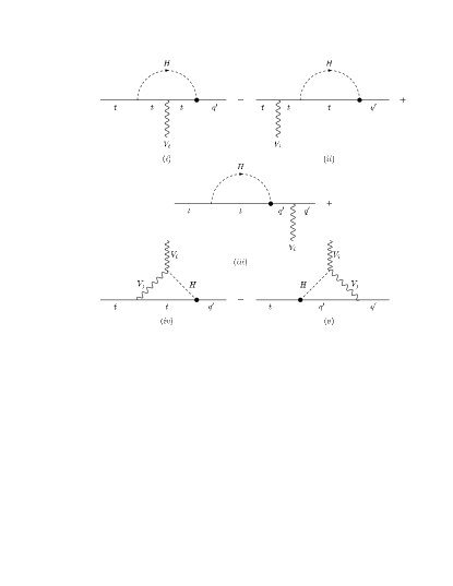
Figure 1: Feynman diagrams contributing to the on-shell $tq^{\prime}V_{i}$ $(V_{i}=\gamma,g,Z$ and $q^{\prime}=u,c)$ vertices in the $m_{q^{\prime}}=0$ approximation. The diagrams (iv) and (v), which only contribute to the $tq^{\prime}Z$ vertex, were evaluated using the unitary gauge.

In the $m_{q^{\prime}}=0$ approximation, which will be used whenever possible, the $tq^{\prime}V$ vertex arises from the Feynman diagrams shown in Fig. 1. The $tq^{\prime}\gamma$ and $tq^{\prime}g$ couplings are induced by the (i)-(iii) diagrams, whereas the $tq^{\prime}Z$ vertex receives additional contributions from the (iv) and (v) graphs. The contributions to the $\kappa_{tq^{\prime}\gamma}$ and $\widetilde{\kappa}_{tq^{\prime}\gamma}$ coefficients can be written as follows:

$$\kappa_{tq^{\prime}\gamma}=-\frac{2Q_{t}\sqrt{\alpha}}{(4\pi)^{3/2}s_{2W}x}\,\epsilon_{tq^{\prime}H}\,A(y)$$ (8)

$$\widetilde{\kappa}_{tq^{\prime}\gamma}=-\frac{2iQ_{t}\sqrt{\alpha}}{(4\pi)^{3/2}s_{2W}x}\,\widetilde{\epsilon}_{tq^{\prime}H}\,A(y),$$ (9)

with $Q_{t}=2/3$, $x=m_{Z}/m_{t}$, $y=m_{H}/m_{t}$, and $A(y)$ the loop function given by

$$A(y)=\frac{1}{2}+2m^{2}_{t}C_{0}+(2-y^{2})\left(B_{0}(2)-B_{0}(1)\right).$$ (10)

where $C_{0}=C_{0}(m^{2}_{t},0,0,m^{2}_{t}y^{2},m^{2}_{t},m^{2}_{t})$, $B_{0}(1)=B_{0}(0,m^{2}_{t},m^{2}_{t}y^{2})$, and $B_{0}(2)=B_{0}(m^{2}_{t},m^{2}_{t},m^{2}_{t}y^{2})$ are Passarino-Veltman scalar functions written in the usual notation.

The contributions to $\kappa_{tq^{\prime}g}$ and $\widetilde{\kappa}_{tq^{\prime}g}$, follow easily after the $g_{s}\lambda^{\alpha}/2$ factor is included into the $\kappa_{tq^{\prime}\gamma}$ and $\widetilde{\kappa}_{tq^{\prime}\gamma}$ coefficients. As for the coefficients associated with the $tq^{\prime}Z$ vertex, they are

$$v_{tq^{\prime}Z}=-\frac{\sqrt{\alpha}}{(4\pi)^{3/2}xs_{2W}}\left[g^{q^{\prime}}_{V}\epsilon_{tq^{\prime}H}A_{1}(x,y)-ig^{q^{\prime}}_{A}\widetilde{\epsilon}_{tq^{\prime}H}A_{2}(x,y)\right],$$ (11)

$$a_{tq^{\prime}Z}=-\frac{\sqrt{\alpha}}{(4\pi)^{3/2}xs_{2W}}\left[g^{q^{\prime}}_{A}\epsilon_{tq^{\prime}H}A_{2}(x,y)-ig^{q^{\prime}}_{V}\widetilde{\epsilon}_{tq^{\prime}H}A_{1}(x,y)\right]$$ (12)

$$\kappa_{tq^{\prime}Z}=\frac{\sqrt{\alpha}}{(4\pi)^{3/2}xs_{2W}}\left[g^{q^{\prime}}_{V}\epsilon_{tq^{\prime}H}A_{3}(x,y)+ig^{q^{\prime}}_{A}\widetilde{\epsilon}_{tq^{\prime}H}A_{4}(x,y)\right],$$ (13)

$$\widetilde{\kappa}_{tq^{\prime}Z}=\frac{i\sqrt{\alpha}}{(4\pi)^{3/2}xs_{2W}}\Big{[}g^{q^{\prime}}_{A}\epsilon_{tq^{\prime}H}A_{4}(x,y)+ig^{q^{\prime}}_{V}\widetilde{\epsilon}_{tq^{\prime}H}A_{3}(x,y)\Big{]},$$ (14)

where $g^{q^{\prime}}_{V}=1/2-(4/3)s^{2}_{W}$ and $g^{q^{\prime}}_{A}=1/2$. The $A_{i}$ functions are given by

$$A_{1}(x,y)=\frac{x^{2}}{\chi^{3}}\left[f^{1}_{0}+\sum^{8}_{i=1,i\neq 3,6}f^{1}_{i}B_{0}(i)+m^{2}_{t}\sum^{3}_{i=1}g^{1}_{i}C_{0}(i)\right],$$ (15)

$$A_{2}(x,y)=\frac{1}{\chi^{3}}\left[f^{2}_{0}+\sum^{8}_{i=1}f^{2}_{i}B_{0}(i)+m^{2}_{t}\sum^{3}_{i=1}g^{2}_{i}C_{0}(i)\right],$$ (16)

$$A_{3}(x,y)=\frac{1}{\chi^{3}}\left[f^{3}_{0}+\sum^{8}_{i=1,i\neq 3}f^{3}_{i}B_{0}(i)+m^{2}_{t}\sum^{3}_{i=1}g^{3}_{i}C_{0}(i)\right],$$ (17)

$$A_{4}(x,y)=\frac{1}{\chi^{3}}\left[f^{4}_{0}+\sum^{8}_{i=1}f^{4}_{i}B_{0}(i)+m^{2}_{t}\sum^{3}_{i=1}g^{4}_{i}C_{0}(i)\right],$$ (18)

with $\chi=1-x$. The $B_{0}(i)$ and $C_{0}(i)$ scalar functions together with the $f^{a}_{i}$ and $g^{a}_{i}$ coefficients are presented in an Appendix. As a crosscheck, we have verified that the amplitude for the $t\to q^{\prime}Z$ decay reproduces that associated with $t\to q^{\prime}\gamma$ when $g^{q^{\prime}}_{V}=1$, $g^{q^{\prime}}_{A}=0$, and $x=0$.

It is straightforward to show that $\sum^{8}_{i=1}f^{j}_{i}=0$ for $j=1\ldots 4$, which means that all of the amplitudes are free of ultraviolet divergences. Thus, after introducing the Yukawa-like operators it is not necessary to use a renormalization scheme. This is due to the fact that the $tq^{\prime}H$ vertex has a renormalizable structure.

It is interesting to analyze the dependence of the loop amplitudes on the Higgs boson mass $m_{H}$. They are shown in Fig. 2 for very large $m_{H}$ and in Fig. 3 in the intermediate $m_{H}$ regime. The decoupling nature of the loop amplitudes is evident in Fig. 2. Also, since these amplitudes vary smoothly with increasing $m_{H}$, as observed in Fig. 3, the corresponding decay widths will show the same behavior. We can also infer the sensitivity of the $tq^{\prime}V_{i}$ vertices to the $tq^{\prime}H$ coupling. From Fig. 3 we can observe that $|A_{1}|\sim 4|A|$, $|A_{2}|\sim 6|A|$, $|A_{3}|\sim|A|$, and $|A_{4}|\sim|A|/2$, with $|A|$ ranging from 0.5 to 0.42. This means that the coefficients $a_{tq^{\prime}Z}$ and $v_{tq^{\prime}Z}$ associated with the $tq^{\prime}Z$ vertex are the most sensitive to the $tq^{\prime}H$ vertex.

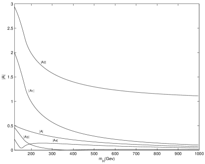
Figure 2: The behavior of the $t\to cV_{i}$ loop amplitudes for a very heavy Higgs boson.

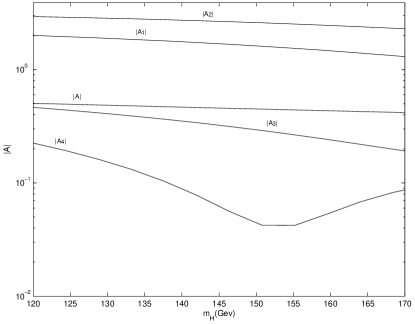
Figure 3: The same as in Fig. 2, but for 120 GeV $\leq m_{H}\leq$170 GeV.

IV Numerical results and discussion

We turn to the numerical results for the $t\to q^{\prime}V_{i}$ and $t\to q^{\prime}H$ branching ratios. In terms of the coefficients of the effective Lagrangian (1), the branching ratios can be written as

$$Br(t\to q^{\prime}\gamma)=\frac{\alpha}{2}\left(\frac{m_{t}}{\Gamma_{t}}\right)\left(|\kappa_{tq^{\prime}\gamma}|^{2}+|\widetilde{\kappa}_{tq^{\prime}\gamma}|^{2}\right),$$ (19)

$$Br(t\to q^{\prime}g)=\frac{2\alpha_{s}}{3}\left(\frac{m_{t}}{\Gamma_{t}}\right)\left(|\kappa_{tq^{\prime}g}|^{2}+|\widetilde{\kappa}_{tq^{\prime}g}|^{2}\right),$$ (20)

where $\Gamma_{t}$ is the total top quark width.

As for the $t\to q^{\prime}Z$ decay, its branching ratio can be written as

$$Br(t\to q^{\prime}Z) = \frac{\alpha}{4s^{2}_{2W}}\left(\frac{m_{t}}{\Gamma_{t}}\right)(1-x^{2})^{2}\Bigg{\{}\frac{1+2x^{2}}{x^{2}}\left(|v_{tq^{\prime}Z}|^{2}+|a_{tq^{\prime}Z}|^{2}\right)$$ (21)

$$-6Re(v_{tq^{\prime}Z}\kappa^{*}_{tq^{\prime}Z}+a_{tq^{\prime}Z}\widetilde{\kappa}^{*}_{tq^{\prime}Z})+(2+x^{2})\left(|\kappa_{tq^{\prime}Z}|^{2}+|\widetilde{\kappa}_{tq^{\prime}Z}|^{2}\right)\Bigg{\}}.$$

whereas for the $t\to q^{\prime}H$ decay we have

$$Br(t\to q^{\prime}H)=\frac{1}{16\pi}\left(\frac{m_{t}}{\Gamma_{t}}\right)\left(1-y^{2}\right)^{2}\left(|\epsilon_{tq^{\prime}H}|^{2}+|\widetilde{\epsilon}_{tq^{\prime}H}|^{2}\right),$$ (22)

which is a tree level prediction in the effective theory.

The $t\to cV_{i}$ and $t\to cH$ branching ratios depend on $m_{H}$ and $\Lambda$, for which we will consider the ranges $120$ GeV $\leq m_{H}\leq 170$ GeV and 400 GeV $\leq\Lambda\leq 1000$ GeV. In Fig. 4, we show the $t\to cV_{i}$ and $t\to cH$ branching ratios versus the Higgs boson mass in the scenario in which $\Lambda=400$ GeV. Since they are proportional to $1/\Lambda^{2}$, the results for other values of $\Lambda$ can be easily obtained from this figure. We can see that all these branching ratios, but $Br(t\to cH)$, vary smoothly in the range considered for the Higgs boson mass. The most pronounced variation of this channel is due to phase space. We can also observe that the branching ratios for the $t\to cg$, $t\to c\gamma$, $t\to cZ$, and $t\to cH$ channels can reach the maximal values $3.4\times 10^{-6}$, $1.7\times 10^{-7}$, $2.4\times 10^{-5}$, and $2\times 10^{-3}$, respectively. Finally, Figs. 5 and 6 show these branching ratios as functions of $\Lambda$ for $m_{H}=120$ GeV and $m_{H}=170$ GeV.

Figure 4: $t\to cV_{i}$ and $t\to cH$ branching ratios as functions of $m_{H}$ for $\Lambda=400$ GeV.

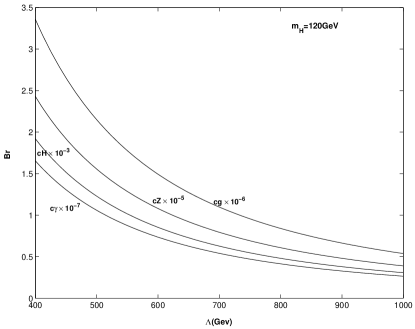
Figure 5: $t\to cV_{i}$ and $t\to cH$ branching ratios as functions of $\Lambda$ for $m_{H}=120$ GeV.

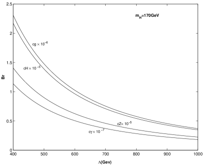
Figure 6: The same as in Fig. 5 but for $m_{H}=170$ GeV.

It is worth comparing our results with those obtained in some specific models. Although in the SM the FCNC top quark decays are strongly suppressed, they may be considerably enhanced in some of its extensions TOPP . For instance, in the THDM-III the $t\to cV_{i}$ and $t\to cH$ (with $H$ a SM-like Higgs boson) decays can have large branching ratios REINA2 ; THDMH , which are several orders of magnitude above the SM ones. SUSY models with universal soft breaking predict branching ratios which are of the same order of magnitude than the SM ones, but this situation is improved when the universality is relaxed by allowing a large flavor mixing between the second and third families, in which case branching ratios as large as $Br(t\to cg)\sim 10^{-6}$, $Br(t\to c\gamma)\sim 10^{-8}$, and $Br(t\to cZ)\sim 10^{-8}$ can be reached MSSM , which however are still too small to be detected. On the contrary, SUSY models with broken $R$-parity may yield enhanced FCNC top quark decays SUSYV ; SUSYH . This has been summarized in Table 1, where we show our predictions for the FCNC top quark decays along with those obtained in some specific models. Compared with the THDM-III predictions, the ELA prediction for the $t\to cg$ branching ratio is almost two orders of magnitude lower, whereas $Br(t\to c\gamma)$ is of the same order, and $Br(t\to cZ)$ is larger by more than one order of magnitude. In contrast, the ELA prediction for $Br(t\to cH)$ is three orders of magnitude larger than in the THDM-III. As far as SUSY models with broken $R$-parity are concerned, their predictions for the $t\to cV_{i}$ decays are all higher than the ELA results, but the respective prediction for the $Br(t\to cH)$ is below.

Table 1: Branching ratios for the $t\to cH$ and $t\to cV_{i}$ decays in the SM and some of its extensions. The effective Lagrangian predictions are displayed in the last two columns for $\Lambda=400$ and $1000$ GeV. The values shown in each column correspond to $m_{H}=120$ GeV and $m_{H}=170$ GeV, respectively.

Decay	SM	THDM-III	SUSY	ELA ($\Lambda=400$)	ELA ($\Lambda=1000$)
$t\to cg$	$5\cdot 10^{-11}$	$10^{-4}-10^{-8}$	$\sim 10^{-3}$	$3.4\times 10^{-6}-2.3\times 10^{-6}$	$5.4\times 10^{-7}-3.7\times 10^{-7}$
$t\to c\gamma$	$5\times 10^{-13}$	$10^{-7}-10^{-12}$	$\sim 10^{-5}$	$1.7\times 10^{-7}-1.1\times 10^{-7}$	$2.6\times 10^{-8}-1.8\times 10^{-8}$
$t\to cZ$	$\sim 10^{-13}$	$10^{-6}-10^{-8}$	$\sim 10^{-4}$	$2.4\times 10^{-5}-1.4\times 10^{-5}$	$3.9\times 10^{-6}-2.3\times 10^{-6}$
$t\to cH$	$10^{-14}-10^{-13}$	$\sim 10^{-6}$	$\sim 10^{-4}$	$2\times 10^{-3}-2.2\times 10^{-5}$	$3.1\times 10^{-4}-3.5\times 10^{-6}$

It is important to comment on the main differences between the scenario arising in those models with an extended scalar sector and that scenario considered so far, in which Higgs-mediated FCNCs arise from virtual effects of heavy particles. As already mentioned, the most popular example of those models with extended scalar sectors is the THDM considered in Ref. REINA1 . In that model, dubbed THDM-III, it is assumed that the SM-like Higgs boson couples diagonally to the fermions at the tree level, so the $t\to cH$ decay proceeds at the one-loop level due to the exchange of virtual $h$, $A$ and $H^{\pm}$ Higgs bosons, which in turn do have nondiagonal couplings to the fermions. As a consequence, the respective branching ratio for the $t\to cH$ decay is lower than in the scenario considered in this work. Although in the THDM-III the $t\to ch$ and $t\to cA$ decays can arise at tree-level and may have large branching ratios, it is possible that the $h$ and $A$ Higgs bosons were so heavy that these decays would not be kinematically allowed. As for the $t\to cV_{i}$ decays, they are induced by loops carrying the $h$ and $A$ Higgs bosons. The Feynman diagrams are similar to those shown in Fig. 1, although there is no contribution from the (iv) and (v) diagrams, which are not induced in the model considered in Ref. REINA1 because the neutral Higgs bosons responsible for FCNC effects do not couple to the $Z$ boson at tree level as they do not receive a VEV.

We now would like to discuss on the possible detection of the FCNC top quark decays at the LHC, which will operate as a top quark factory, with a production of about $10^{8}$ $t\bar{t}$ events per year. The dominant mechanism for top quark pair production is through $q\bar{q}$ or $gg$ annihilation, whereas single top quark events can be produced through electroweak processes such as $Wg$ fusion or the production of a virtual $W$ boson decaying into $t\bar{b}$. In this case, the cross section is about $1/3$ that of $t\bar{t}$ production. Although the observability of a particular channel decay depends on several factors, in a purely statistical basis those channels with branching ratios larger than about $10^{-6}-10^{-7}$ do have the chance of being detected. However, background problems and systematics may reduce this value by several orders of magnitude depending on the particular signature. For instance, the $t\to cg$ mode would require a large branching ratio in order to be detected as it is swamped by hadronic backgrounds. As far as the $t\to c\gamma$, $t\to cZ$, and $t\to cH$ decays are concerned, they could be detected even with relatively small branching ratios because they would be produced in a cleaner environment. The LHC will have a sensitivity of about $2\times 10^{-4}$ and $3.4\times 10^{-5}$ to the $t\to cZ$ and $t\to c\gamma$ decays, respectively TOPP , whereas the sensitivity to $t\to cH$ can be up to $6.5\times 10^{-5}$ AS . From the results presented in Fig. 4 and Table 1 we can conclude that the $t\to c\gamma$ and $t\to cZ$ decays would hardly be detected at the LHC. A similar situation is expected for the $t\to cg$ mode due to background problems, but the $t\to cH$ decay seems to be more promising. As far as the FCNC top transitions involving the $u$ quark are concerned, they are suppressed by a factor of $m_{u}/m_{c}$ and are far from the reach of the LHC.

Finally, we consider that our estimation for the strength of the $tq^{\prime}H$ vertex, in which the $\Lambda$ scale was introduced instead of the Fermi one, is realistic since it describes more appropriately any possible scenario arising from the underlying physics responsible for FCNC effects. We believe that this is an interesting situation as a deep link between flavor physics and symmetry breaking is possible, thereby favoring this type of processes.

V Conclusions

The copious production of top quark events expected at the LHC, together with the possibility of detecting the Higgs boson at this collider, constitute an incentive for studying Higgs-mediated FCNC top transitions. Due to the large mass of the top quark and the Higgs boson, the top-Higgs dynamics is expected to provide a unique scenario to probe the physics beyond the electroweak scale. This possibility has been explored in a model-independent manner using the effective Lagrangian technique. Under the assumption that FCNC top transitions are predominantly induced by the Higgs boson, the most general Yukawa sector extended with dimension-six operators, which generates the most general CP-even and CP-odd $tq^{\prime}H$ vertex, was studied. We adopted a slightly modified version of the Cheng-Sher ansatz to estimate the size of the $tq^{\prime}H$ vertex. This ansatz comprises three scales: $m_{q^{\prime}}$, $m_{t}$, and the new physics scale $\Lambda$. The most promising results are obtained when $\Lambda$ is close to the Fermi scale. The main differences with the scenario arising in models with extended scalar sectors were emphasized. One of the most remarkably features of the scenario considered in this work is the fact that the $t\to q^{\prime}H$ decay (with $H$ the SM Higgs boson) arises at the tree level. It turns out that the top quark decay widths depend only on the Higgs boson mass and the new physics scale, and for intermediate values of $\Lambda$ they do not change appreciably when $m_{H}$ ranges from 120 GeV to 170 GeV. In such a scenario, the $t\to cg$, $t\to c\gamma$, and $t\to cZ$ decays have branching ratios several orders of magnitude larger than the ones predicted by the SM, but not large enough to be detected at the LHC. As far as the $t\to cH$ decay is concerned, its branching ratio may be up to $10^{-3}$, which is at the reach of the LHC. This result is three orders of magnitude larger than the THDM-III prediction and one order larger than in SUSY models with broken $R$-parity. As for the decays with the $c$ quark replaced by the $u$ one, the respective branching ratios are smaller by a factor of $m_{u}/m_{c}$, and thus they would be out of the LHC reach.

Appendix A $tq^{\prime}Z$ loop amplitudes

The scalar functions and the coefficients $f^{a}_{i}$ and $g^{a}_{i}$ appearing in the $tq^{\prime}Z$ loop amplitudes are

$$B_{0}(1) = B_{0}(0,0,m^{2}_{t}x^{2}),$$

$$B_{0}(2) = B_{0}(m^{2}_{t},0,m^{2}_{t}y^{2}),$$

$$B_{0}(3) = B_{0}(0,m^{2}_{t},m^{2}_{t}x^{2}),$$

$$B_{0}(4) = B_{0}(0,m^{2}_{t}y^{2},m^{2}_{t}),$$

$$B_{0}(5) = B_{0}(m^{2}_{t}x^{2},m^{2}_{t},m^{2}_{t}),$$

$$B_{0}(6) = B_{0}(m^{2}_{t},m^{2}_{t},m^{2}_{t}x^{2}),$$

$$B_{0}(7) = B_{0}(m^{2}_{t}x^{2},m^{2}_{t}y^{2},m^{2}_{t}x^{2}),$$

$$B_{0}(8) = B_{0}(m^{2}_{t},m^{2}_{t}y^{2},m^{2}_{t}),$$ (23)

$$C_{0}(1) = C_{0}(m^{2}_{t},0,m^{2}_{t}x^{2},m^{2}_{t},m^{2}_{t}y^{2},m^{2}_{t}),$$

$$C_{0}(2) = C_{0}(m^{2}_{t},0,m^{2}_{t}x^{2},m^{2}_{t}x^{2},m^{2}_{t},m^{2}_{t}y^{2}),$$

$$C_{0}(3) = C_{0}(m^{2}_{t},0,m^{2}_{t}x^{2},m^{2}_{t}y^{2},0,m^{2}_{t}x^{2}),$$ (24)

$$f^{1}_{0} = \frac{1}{2}\chi^{2},$$

$$f^{1}_{1} = 2\chi^{2},$$

$$f^{1}_{2} = 2(1-x^{4}),$$

$$f^{1}_{7} = -4x^{2}\chi,$$

$$f^{1}_{4} = \frac{1}{2}\chi\left[x^{2}(y^{2}-3)-2(2y^{2}-3)\right],$$

$$f^{1}_{5} = -\frac{1}{2}\left[x^{4}-(2y^{2}+5)x^{2}-2(2y^{2}-5)\right],$$

$$f^{1}_{8} = -\frac{1}{2}\left[x^{4}(y^{2}-4)+x^{2}(14-3y^{2})+8(y^{2}-2)\right],$$ (25)

$$g^{1}_{1} = 2x^{4}+x^{2}(y^{4}+2y^{2}-7)+2(y^{2}-2)^{2},$$

$$g^{1}_{2} = 2\chi^{3},$$

$$g^{1}_{3} = 2x\chi\left(x^{4}+\chi y^{2}+\right),$$ (26)

$$f^{2}_{0} = \frac{3}{2}x^{2}\chi^{2},$$

$$f^{2}_{1} = -2x^{2}\chi^{2},$$

$$f^{2}_{2} = -2x^{2}(x^{4}-1),$$

$$f^{2}_{3} = \chi^{3},$$

$$f^{2}_{4} = -\frac{1}{2}\chi\left[-x^{4}(y^{2}-3)+2x^{2}(y^{2}-4)+2(y^{2}+1)\right],$$

$$f^{2}_{5} = -\frac{1}{2}x^{2}(x^{2}+2)(x^{2}-2y^{2}+1),$$

$$f^{2}_{6} = -3x^{4}+x^{2}(4y^{2}-3)+2y^{2},$$

$$f^{2}_{7} = 4x^{6}-x^{4}(y^{2}-2)-5x^{2}y^{2},$$

$$f^{2}_{8} = \frac{1}{2}\left[x^{6}(y^{2}-4)+x^{4}(14-3y^{2})-2x^{2}(y^{2}+4)-2(y^{2}-2)\right],$$ (27)

$$g^{2}_{1} = -2x^{6}+x^{4}(y^{4}-2y^{2}+7)+2x^{2}(y^{4}-2y^{2}-2)+2,$$

$$g^{2}_{2} = 2\left[-x^{8}+x^{6}(y^{2}+3)-4x^{4}y^{2}+x^{2}(2y^{4}-3y^{2}+1)+y^{4}\right],$$

$$g^{2}_{3} = -2x^{2}\chi(x^{4}+x^{2}y^{2}-y^{2}+1),$$ (28)

$$f^{3}_{0} = \frac{1}{2}\chi^{2},$$

$$f^{3}_{1} = 2x^{2}\chi^{2},$$

$$f^{3}_{2} = 4x^{2}\chi,$$

$$f^{3}_{6} = 2x^{2}\chi^{2},$$

$$f^{3}_{4} = -\frac{1}{2}\chi\left[x^{2}(y^{2}+1)+2(y^{2}-2)\right],$$

$$f^{3}_{5} = \frac{1}{2}x^{2}(5x^{2}+6y^{2}-11),$$

$$f^{3}_{7} = -4x^{4}\chi,$$

$$f^{3}_{8} = \frac{1}{2}\left[x^{4}(y^{2}-4)+x^{2}(6-5y^{2})-2(y^{2}-2)\right],$$ (29)

$$g^{3}_{1} = 2x^{4}(2y^{2}-1)+x^{2}(3y^{4}-10y^{2}+3)+2,$$

$$g^{3}_{2} = 2x^{2}(y^{2}-1)\chi^{2},$$

$$g^{3}_{3} = 2x^{2}\chi\left[x^{2}(y^{2}+1)-y^{2}+1\right],$$ (30)

$$f^{4}_{0} = -\frac{3}{2}\chi^{2},$$

$$f^{4}_{1} = 2x^{2}\chi^{2},$$

$$f^{4}_{2} = 4x^{2}\chi,$$

$$f^{4}_{3} = -\chi^{3},$$

$$f^{4}_{4} = \frac{1}{2}\chi\left[x^{2}(y^{2}+1)-2(2y^{2}-1)\right],$$

$$f^{4}_{5} = -\frac{1}{2}\left[x^{4}+x^{2}(6y^{2}-11)+4\right],$$

$$f^{4}_{6} = -x^{6}+3x^{4}-2x^{2}(y^{2}-2)-4y^{2},$$

$$f^{4}_{7} = -8x^{4}+x^{2}(5y^{2}+2)+y^{2},$$

$$f^{4}_{8} = -\frac{1}{2}\left[x^{4}(y^{2}-4)-x^{2}(5y^{2}-14)-2(y^{2}+2)\right],$$ (31)

$$g^{4}_{1} = -(y^{2}-1)\left[2x^{4}+x^{2}(3y^{2}-7)+2\right],$$

$$g^{4}_{2} = -2\left[(y^{2}-1)x^{6}-2(y^{2}-2)x^{4}+y^{2}(y^{2}-5)x^{2}+2y^{4}\right],$$

$$g^{4}_{3} = 2x^{2}\chi\left[x^{2}(y^{2}+1)-y^{2}+1\right].$$ (32)