Hard exclusive processes and higher-order QCD corrections

Abstract

The short review of the higher order corrections to the hard exclusive processes is given. Different approaches are discussed and the importance of higher-order calculations is stressed.

1 Introduction

Quantum Chromodynamics (QCD) offers the description of hadrons in terms of quarks and gluons. There are two basic ingredients of that picture: bound state dynamics of hadrons and fundamental interactions of quarks and gluons. While the former is still rather elusive to existing theoretical tools, the latter is rather well understood. The description of the hadronic processes at large momentum transfer is realized by making use of the factorization of high and low energy (short and long distance) dynamics. The existence of asymptotic freedom makes then the high energy part tractable to the perturbative calculation, i.e., the perturbative QCD (PQCD).

Exclusive processes are defined as the scattering reactions in which the kinematics of all initial and final state particles are specified, like, for example, the processes defining the hadron form factors ($\gamma^{*}\gamma^{(*)}\to\pi$, $\gamma^{*}\pi\to\pi$, $\gamma^{*}\to\pi\pi$, $ep\rightarrow ep$, $\cdots$ ), the two-photon annihilation processes ($\gamma\gamma\to\pi\pi$, $\gamma\gamma\rightarrow\overline{p}p$, $\cdots$ ), the hadron scatterings ($\pi p\rightarrow\pi p$, $pp\rightarrow pp$, $\cdots$ ), the decays of heavy hadrons ( $J/\psi\rightarrow\pi\pi\pi$, $B\to\pi\pi$, $\cdots$ ) etc. The hard exclusive reactions, i.e., the exclusive reactions at large momentum transfer (or wide-angle), can be described by the so-called hard-scattering picture HSP ; LepageB80 . The basis of this picture is the factorization of short and long distance dynamics, i.e, the factorization of the hard-scattering amplitude into the elementary hard-scattering amplitude and hadron distribution amplitudes one for each hadron involved in the process. Usually the following standard approximations are made. Hadron is replaced by the valent Fock state, collinear approximation, in which hadron constituents are constrained to be collinear, is adopted, and the masses are neglected. For example, in the case of the pion this leads to replacing the pion by $\left|\pi\right>\rightarrow\left|q\overline{q}\right>$ (correct flavour structure has to be taken into account), adopting $p_{q}=x\>{p}$, $p_{\overline{q}}=(1-x)p$, where $p$, $p_{q}$ and $p_{\overline{q}}$ are pion, quark and antiquark momenta, respectively, while $0<x<1$ is the longitudinal momentum fraction, and taking $m_{q}=m_{\overline{q}}=0\>,m_{\pi}=0$.

Generally, the hard-scattering amplitude is then represented by the following convolution formula:

$${\cal M}(Q^{2})=\int_{0}^{1}[dx]\quad{T_{H}}(x_{j},\,{Q^{2}},\,\mu_{F}^{2})\quad{\prod_{{h}_{i}}}\,\Phi_{{h}_{i}}(x_{j},\,\mu_{F}^{2})\,,$$ (1)

$$[dx]=\prod_{j=1}^{{n}_{h_{i}}}dx_{j}\,\delta(1-\sum_{k=1}^{{n}_{h_{i}}}x_{k})\,,$$

where $T_{H}$ is the process-dependent elementary hard-scattering amplitude, $\Phi_{{h}_{i}}$ is the process-independent distribution amplitude (DA) of the hadron ${h}_{i}$, $Q^{2}$ denotes the large momentum transfer while $\mu_{F}^{2}$ is the factorization scale at which the separation between short and long distance dynamics takes place.

Within this framework leading-order (LO) predictions have been obtained for many exclusive processes. It is well known, however, that, unlike in QED, the LO predictions in PQCD do not have much predictive power, and that higher-order corrections are essential for many reasons. In general, they have a stabilizing effect reducing the dependence of the predictions on the schemes and scales. Therefore, to achieve a complete confrontation between theoretical predictions and experimental data, it is very important to know the size of radiative corrections to the LO predictions.

The list of exclusive processes at large momentum transfer analyzed at next-to-leading order (NLO) is very short and includes only three processes: the meson electromagnetic form factor FieldGOC81 ; DittesR81 ; Sarmadi82 ; KhalmuradovR85 ; KadantsevaMR86 ; BraatenT87 ; MNP99 , the meson transition form factor AguilaC81 ; Braaten83 ; KadantsevaMR86 ; KrollP02 , and the process $\gamma\gamma\rightarrow M\overline{M}$ ($M=\pi$, $K$) Nizic87 .

We note here that the meson transition form factor belongs to the same class of processes as the deeply virtual Compton scattering (DVCS) MullerRGDH94 ($\gamma^{*}p\rightarrow\gamma^{*}p$), which recently has been extensively studied in the context of general parton distributions (GPDs) DVCS . Regarding the elementary hard-scattering amplitude, these two processes, or correspondingly subprocesses $\gamma^{*}\gamma^{*}\rightarrow(q\bar{q})$ and $\gamma^{*}q\rightarrow\gamma^{*}q$, differ only in kinematic region and are related by crossing. Still, the NLO correction to DVCS has been calculated independently MankiewiczPSVW98 ; JiO98 ; BelitskyM98 . Analogous connection exists between the pion electromagnetic form factor and the deeply virtual electroproduction of mesons (DVEM) DVEM ($\gamma^{*}p\rightarrow Mp$, the momentum transfer $t$ between the initial and the final proton is negligible, while the virtuality of the photon is large). In the context of subprocesses, there is a connection between $\gamma^{*}(q\bar{q})\rightarrow(q\bar{q})$ and $\gamma^{*}q\rightarrow(q\bar{q})q$. In BelitskyM01 the use has been made of the NLO results for the pion electromagnetic form factor to obtain the NLO prediction for the specific case of DVEM (electroproduction of the pseudoscalar flavour non-singlet mesons). In this work we mostly discuss the meson form factor calculations.

At the next-to-next-to-leading order (NNLO) only the $\beta_{0}$-proportional terms for the deeply virtual Compton scattering and pion transition form factor have been explicitly calculated BelitskySch98 ; MNP01 . The use of conformal constraints made it possible to circumvent the explicit calculation and to obtain the full NNLO results for the pion transition form factor MelicMP02 .

Finally, let us note that apart from the deeply virtual region, also the wide angle region has been investigated in the literature in the context of the Compton scattering (WACS), as well as, electroproduction of mesons (WAEM) HuangK00 . The NLO corrections were calculated only for the WACS HuangKM01 ; HuangM03 .

In this paper the introduction to hard-scattering picture for exclusive processes is given in Sec. 2. The characteristic properties of the PQCD predictions regarding the importance of higher-order corrections and the renormalization scale ambiguities are explained in Sec. 3. Section 4 is devoted to the short review of exclusive processes calculated to the next-to-leading order (NLO) in the strong coupling constant $\alpha_{S}$: meson electromagnetic form factor ($\gamma^{*}M\rightarrow M$), photon-to-meson transition form factor ($\gamma^{*}\gamma^{(*)}\rightarrow M$), meson pair production: $\gamma\gamma\rightarrow M\bar{M}$. In Sec. 5 the next-to-next-to-leading order (NNLO) prediction for the photon-to-pion transition form factor obtained using conformal symmetry constraints is explained. Finally, in Sec. 6 the summary and conclusions are given.

2 Introduction to the hard-scattering picture

Let us explain the basic ingredients of the standard hard-scattering picture by taking as an example the simplest exclusive quantity, i.e., the photon-to-pion transition form factor $F_{\pi\gamma^{(*)}}$ appearing in the amplitude of the process ${\gamma^{*}}(q_{1},\mu){\gamma^{(*)}}(q_{2},\nu)\rightarrow\pi(p)$. At least one photon virtuality has to be large and we take here the simple case : $-q_{1}^{2}=Q^{2}\gg$ and $q_{2}^{2}=0$. The full amplitude is of the form

$$\Gamma^{\mu}=i\,e^{2}\;F_{\pi\gamma}(Q^{2})\;\varepsilon^{\mu\nu\alpha\beta}\;q_{1\alpha}q_{2\beta}\;\epsilon_{\nu}(q_{2})\,,$$ (2)

and the transition form factor can be represented by a convolution

$$F_{\pi\gamma}(Q^{2})=T_{H}(x,Q^{2},\mu_{F}^{2})\,\otimes\,\Phi(x,\mu_{F}^{2})\,.$$ (3)

Here $A(x)\otimes B(x)\equiv\int_{0}^{1}dxA(x)B(x)$ and $\mu_{F}^{2}$ is a factorization scale.

The elementary hard-scattering amplitude $T_{H}$ obtained from $\gamma^{*}\,\gamma\rightarrow q\overline{q}$ is calculated using the PQCD. By definition, $T_{H}$ is free of collinear singularities and has a well–defined expansion in $\alpha_{S}(\mu_{R}^{2})$, with $\mu_{R}^{2}$ being the renormalization (or coupling constant) scale of the hard-scattering amplitude. Thus, one can write

$$T_{H}(x,Q^{2}) = T_{H}^{(0)}(x,Q^{2})+\frac{\alpha_{S}(\mu_{R}^{2})}{4\pi}T_{H}^{(1)}(x,Q^{2},\mu_{F}^{2})$$ (4)

$$+\frac{\alpha_{S}^{2}(\mu_{R}^{2})}{(4\pi)^{2}}T_{H}^{(2)}(x,Q^{2},\mu_{F}^{2},\mu_{R}^{2})+\cdots\,.$$

The diagrams contributing to LO and representative diagrams contributing to NLO order are displayed in Figs. 1 and 2, respectively.

Figure 1: Lowest-order Feynman diagrams contributing to the $\gamma^{*}\gamma\rightarrow q\overline{q}$ amplitude.

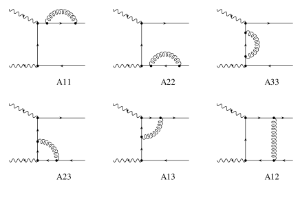
Figure 2: Distinct one-loop Feynman diagrams contributing to $\gamma^{*}\gamma\rightarrow q\overline{q}$.

When evaluating the NLO amplitude one encounters the UV and collinear singularities. The former are removed by coupling constant ($\alpha_{S}$) renormalization introducing the scale $\mu_{R}^{2}$, while the latter are factorized into the DA at the scale $\mu_{F}^{2}$.

The pion distribution amplitude is defined in terms of the matrix elements of composite operators: $\langle 0|\Psi(-z)\gamma^{+}\gamma_{5}\Omega\Psi(z)|\pi\rangle$. While the DA form is taken as an (nonperturbative) input at some lower scale $\mu_{0}^{2}$ ($\Phi(x,\mu_{0}^{2})$), its evolution to the factorization scale $\mu_{F}^{2}$ ($\Phi(x,\mu_{F}^{2})$) is governed by PQCD. The DA can hence be written in a form

$$\Phi(x,\mu_{F}^{2})={\phi_{V}(x,y,\mu_{F}^{2},\mu_{0}^{2})}\otimes\Phi(y,\mu_{0}^{2})\,,$$ (5)

where $\phi_{V}$ denotes the evolution part of the DA. In latter the resummation of $(\alpha_{S}\ln(\mu_{F}^{2}/\mu_{0}^{2}))^{n}$ terms is usually included, and $\phi_{V}$ is obtained by solving the evolution equation

$${\mu_{F}^{2}}\frac{\partial}{\partial{\mu_{F}^{2}}}\phi_{V}=V\,\otimes\,\phi_{V}\>\,,$$ (6)

where

$$V=\frac{\alpha_{S}(\mu_{F}^{2})}{4\pi}V_{1}+\frac{\alpha_{S}^{2}(\mu_{F}^{2})}{(4\pi)}V_{2}+\cdots\>$$ (7)

represents the perturbatively calculable evolution kernel.

One often introduces the distribution amplitude $\phi$ normalized to unity $\int_{0}^{1}dx\;\phi(x,\mu_{F}^{2})=1$, and related to $\Phi(x,\mu_{F}^{2})$ by $\Phi=f_{\pi}/(2\sqrt{2N_{c}})\,\phi\,$ where $f_{\pi}=0.131$ GeV is the pion decay constant and $N_{c}$ is the number of colours. The solutions of the evolution equation (6) combined with the nonperturbative input can then be written in a form of an expansion over Gegenbauer polynomials $C_{n}^{3/2}$ which represent the eigenfunctions of the LO evolution equation:

$$\phi(x,\mu_{F}^{2})=6x(1-x)\left[1+\sum_{n=2}^{\infty}{}^{\prime}B_{n}(\mu_{F}^{2})\;C_{n}^{3/2}(2x-1)\right]\,.$$ (8)

Here $\sum{}^{\prime}$ denotes the sum over even indices. The nonperturbative input $B_{n}(\mu_{0}^{2})$ as well as the evolution is now contained in $B_{n}$ coefficients. They have a well defined expansion in $\alpha_{S}$:

$$B_{n}(\mu_{F}^{2})=B_{n}^{LO}(\mu_{F}^{2})+\frac{\alpha_{S}(\mu_{F}^{2})}{4\pi}B_{n}^{NLO}(\mu_{F}^{2})+\cdots\,,$$ (9)

where

$$B_{n}^{LO}(\mu_{F}^{2})=f(\mu_{F}^{2},\mu_{0}^{2},B_{n}(\mu_{0}^{2}))\,, B_{n}^{NLO}(\mu_{F}^{2})=g(\mu_{F}^{2},\mu_{0}^{2},B_{k(k\leq n)}(\mu_{0}^{2}))\qquad$$ (10)

represent the LO and NLO Muller94etc parts whose exact form in $\overline{\mbox{MS}}$ factorization scheme is given in, for example, MNP99 ; MNP01 .

As the DA input one often takes the asymptotic function

$$\phi_{as}\equiv\phi(x,\infty)=6x(1-x)$$ (11)

being the solution of the DA evolution equation for $\mu_{F}^{2}\to\infty$ and the simplest possibility. We list here two more choices from the literature

$$\begin{array}[]{rl}\phi_{CZ}\mbox{\cite[cite]{\@@bibref{Authors Phrase1YearPhrase2}{ChernyakZ84}{\@@citephrase{(}}{\@@citephrase{)}}}}:&B_{2}(0.25\,\mbox{GeV}^{2})=2/3\,,\\[2.84544pt] \phi_{BMS}\mbox{\cite[cite]{\@@bibref{Authors Phrase1YearPhrase2}{BakulevMS01}{\@@citephrase{(}}{\@@citephrase{)}}}}:&B_{2}(1\,\mbox{GeV}^{2})=0.188\qquad B_{4}(1\,\mbox{GeV}^{2})=-0.13\par\,.\end{array}$$ (12)

The CZ distribution amplitude is nowadays mostly ruled out (see MNP99b and references therein), and it is believed that even at lower energies the pion DA is close to asymptotic form but probably end-point suppressed like the BMS DA.

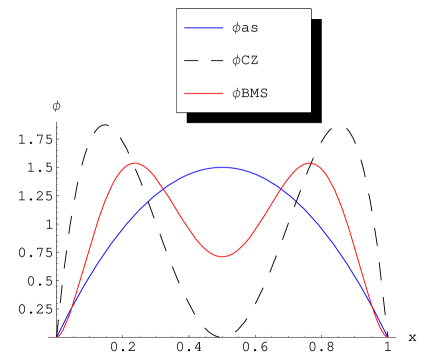
Figure 3: DA candidates.

3 PQCD prediction

In this section we would like to discuss some properties inherent to all PQCD predictions.

Let us first briefly discuss the expansion parameter, i.e., the QCD coupling constant. The QCD $\beta$ function given by

$$\beta(\alpha_{S}(\mu^{2}))=\mu^{2}\frac{\partial}{\partial\mu^{2}}\alpha_{S}(\mu^{2})=-\frac{\alpha_{S}^{2}(\mu^{2})}{4\pi}\beta_{0}-\cdots$$ (13)

is negative ($\beta_{0}=1/3(11N_{c}-2n_{f})$, $n_{f}$ is the number of active flavours) and theory is asymptotically free. The usual one-loop solution of the renormalization group equation (13) is given by

$$\alpha_{S}(\mu^{2})=\frac{4\pi}{\beta_{0}\ln(\mu^{2}/\Lambda^{2})}$$ (14)

and, obviously, $\alpha_{S}(\infty)=0$, while, for example, $\alpha_{S}((1)4\,\mbox{GeV}^{2})\approx(0.43)0.3$, $(\Lambda=0.2\,\mbox{GeV},n_{f}=3)$. Obviously, low-energy behaviour of such $\alpha_{S}$ represents a problem due to the existence of the Landau pole: $\alpha_{S}(\Lambda^{2})\rightarrow\infty$. In the literature one can encounter several prescriptions to improve $\alpha_{S}$ in low-energy region. For example, “frozen” coupling constant

$$\alpha_{S}(\mu^{2})=\frac{4\pi}{\beta_{0}\ln((\mu^{2}+m_{g}^{2})/\Lambda^{2})}$$ (15)

or analytical coupling ShirkovS97

$$\alpha_{S}(\mu^{2})=\frac{4\pi}{\beta_{0}}\left[\frac{1}{\ln(\mu^{2}/\Lambda^{2})}+\frac{\Lambda^{2}}{\Lambda^{2}-\mu^{2}}\right]\,.$$ (16)

But even these improved forms of $\alpha_{S}$ give rather large values at lower energies. Thus, LO QCD predictions do not have much predictive power and higher-order corrections are important.

Generally, the PQCD amplitude can be written in a form

$${\cal M}(Q^{2})={\cal M}^{(0)}(Q^{2})+\frac{\alpha_{S}(\mu_{R}^{2})}{4\pi}{\cal M}^{(1)}(Q^{2})+\frac{\alpha_{S}^{2}(\mu_{R}^{2})}{(4\pi)^{2}}{\cal M}^{(2)}(Q^{2},\mu_{R}^{2})+\cdots\,,$$ (17)

where $Q^{2}$ is some large momentum and as usual $\mu_{R}^{2}$ represents the renormalization scale. The truncation of the perturbative series to finite order introduces the residual dependence of the results on the renormalization scale $\mu_{R}$ and scheme (to the order we are calculating these dependences can be represented by one parameter, say, the scale). Inclusion of higher order corrections decreases this dependence. Nevertheless, we are still left with intrinsic theoretical uncertainty of the perturbative results. One can try to estimate this uncertainty (see, for example, MNP99 ) or one can try to find the “optimal” renormalization scale $\mu_{R}$ (and scheme) on the basis of some physical arguments . In the latter case, one can assess the size of the higher order corrections and of the expansion parameter. These values can then serve as a sensible criteria for the convergence of the expansion.

The simplest and widely used choice for $\mu_{R}$ is $\mu_{R}^{2}=Q^{2}$, and the justification is mainly pragmatic. However, physical arguments suggest that the more appropriate scale $\mu_{R}$ is lower. Namely, since each external momentum entering an exclusive reaction is partitioned among many propagators of the underlying hard-scattering amplitude, the physical scales that control these processes are inevitably much softer than the overall momentum transfer. There are number of suggestions in the literature. According to fastest apparent convergence (FAC) procedure FAC , the scale $\mu_{R}$ is determined by the requirement that the NLO coefficient in the perturbative expansion of the physical quantity in question vanishes, i.e., one demands ${\cal M}^{(2)}(Q^{2},\mu_{R}^{2})=0$. On the other hand, following the principle of minimum sensitivity (PMS) PMS one mimics the independence of the all order expansion on the scale $\mu_{R}$, and one chooses the renormalization scale $\mu_{R}$ at the stationary point of the truncated perturbative series: $d{\cal M}_{\mbox{finite order}}(Q^{2},\mu_{R}^{2})/d\mu_{R}^{2}=0$. In the Brodsky-Lepage-Mackenzie (BLM) procedure BLM83 , all vacuum-polarization effects from the QCD $\beta$-function are resummed into the running coupling constant. According to BLM procedure, the renormalization scale best suited to a particular process in a given order can, in practice, be determined by setting the scale demanding that $\beta$-proportional terms should vanish:

$${\cal M}^{(2)}(Q^{2},\mu_{R}^{2})=\beta_{0}\,{\cal M}^{(2,\beta_{0})}(Q^{2},\mu_{R}^{2})+{\cal M}^{(2,\mbox{rest})}(Q^{2})$$ (18)

and

$${\cal M}^{(2,\beta_{0})}(Q^{2},\mu_{R}^{2})=0\,.$$ (19)

As it is known, the relations between physical observables must be independent of renormalization scale and scheme conventions to any fixed order of perturbation theory. In Ref. BrodskyL95 was argued that applying the BLM scale-fixing to perturbative predictions of two observables in, for example, $\overline{\mbox{MS}}$ scheme and then algebraically eliminating $\alpha_{\overline{MS}}$ one can relate any perturbatively calculable observables without scale and scheme ambiguity, where the choice of BLM scale ensures that the resulting “commensurate scale relation” (CSR) is independent of the choice of the intermediate renormalization scheme. Following this approach, in paper by Brodsky et al.BrodskyJPR98 the several exclusive hadronic amplitudes were analyzed in $\alpha_{V}$ scheme, in which the effective coupling $\alpha_{V}(\mu^{2})$ is defined from the heavy-quark potential $V(\mu^{2})$. The $\alpha_{V}$ scheme is a natural, physically based scheme, which by definition automatically incorporates vacuum polarization effects. The $\mu_{V}^{2}$ scale which then appears in the $\alpha_{V}$ coupling reflects the mean virtuality of the exchanged gluons. Furthermore, since $\alpha_{V}$ is an effective running coupling defined from the physical observable it must be finite at low momenta, and the appropriate parameterization of the low-energy region should in principle be included. The scale-fixed relation between the $\alpha_{\overline{MS}}$ and $\alpha_{V}$ couplings is given by BrodskyJPR98

$$\alpha_{\overline{MS}}(\mu_{BLM}^{2})=\alpha_{V}(\mu_{V}^{2})\left(1+\frac{\alpha_{V}(\mu_{V}^{2})}{4\pi}\,\frac{8C_{A}}{3}+\cdots\right)\,,$$ (20)

where $\alpha_{V}(\mu_{V}^{2})$ is defined from the heavy-quark potential $V(\mu_{V}^{2})$ and

$$\mu_{V}^{2}=e^{5/3}\,\mu_{BLM}^{2}\,.$$ (21)

4 Exclusive processes at higher order: explicit calculations

As mentioned in Sec. 1, only the small number of exclusive processes have been analyzed in higher orders. When higher order calculations are explicitly performed, usually the dimensional regularization together with the $\overline{\mbox{MS}}$ renormalization scheme is applied.

4.1 Photon-to-$\pi$ ($\eta$, $\eta^{\prime}$) transition form factor

The photon-to-$\pi$ transition form factor appearing in the amplitude ${\gamma^{*}}{\gamma}{\rightarrow}{\pi^{0}}$ takes the form of an expansion

$$F_{\pi\gamma}(Q^{2}) = F^{(0)}_{\pi\gamma}(Q^{2})+\frac{\alpha_{S}(\mu_{R}^{2})}{4\pi}F^{(1)}_{\pi\gamma}(Q^{2})$$ (22)

$$+\frac{\alpha_{S}^{2}(\mu_{R}^{2})}{(4\pi)^{2}}\left[\beta_{0}\,F^{(2,\beta_{0})}_{\pi\gamma}(Q^{2},\mu_{R}^{2})+\cdots\right]+\cdots\,,$$

where only the parts that can be found in the literature as explicitly calculated from the contributing Feynman diagrams are written.

There are 2 LO diagrams contributing to the subprocess amplitude $\gamma^{*}\gamma\rightarrow(q\bar{q})$ and displayed in Fig. 1. Furthermore, there are 12 one-loop diagrams contributing at NLO order AguilaC81 ; Braaten83 ; KadantsevaMR86 . The representative diagrams are given in Fig. 2. In the case of the photon-to-$\eta$ ($\eta^{\prime}$) transition form factor the two-gluon states also contribute ($\gamma^{*}\gamma\rightarrow(gg)$) giving rise to 6 more diagrams at NLO KrollP02 . In MNP01 the $\beta_{0}$-proportional NNLO terms were determined from the 12 two-loop Feynman diagrams obtained from the one-loop diagrams by adding the gluon vacuum polarization bubble.

The numerical predictions for $F_{\pi\gamma}(Q^{2})$ are displayed in Fig. 4.

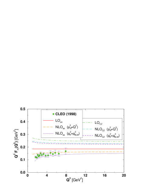
Figure 4: LO and NLO predictions for the photon-to-pion transition form factor.

Obviously, the results obtained using the CZ DA overshoot the experimental data. The BLM scale for the asymptotic DA amounts to $(\mu_{BLM}^{2})^{as}\approx Q^{2}/9$, while $\alpha_{S}\leq 0.5\mbox{ for }Q^{2}>4\mbox{ GeV}^{2}$. In the $\alpha_{V}$ scheme for the coupling constant scale one obtains $(\mu_{V}^{2})^{as}\approx Q^{2}/2$.

4.2 Pion electromagnetic form factor

The spacelike pion electromagnetic form factor $F_{\pi}(Q^{2})$ appearing in the amplitude $\gamma^{*}\pi^{+(-)}\rightarrow\pi^{+(-)}$, takes the form of an expansion

$$F_{\pi}(Q^{2})=\frac{\alpha_{S}(\mu_{R}^{2})}{4\pi}F^{(1)}_{\pi}(Q^{2})+\frac{\alpha_{S}^{2}(\mu_{R}^{2})}{(4\pi)^{2}}F^{(2)}_{\pi}(Q^{2},\mu_{R}^{2})+\cdots\,.$$ (23)

There are 4 diagrams that contribute to the amplitude $\gamma^{*}(q_{1}\bar{q_{2}})\rightarrow(q_{1}\bar{q_{2}})$ at LO (see Fig. 5), and 62 one-loop diagrams at NLO FieldGOC81 ; DittesR81 ; Sarmadi82 ; KhalmuradovR85 ; BraatenT87 ; KadantsevaMR86 ; MNP99 (see Fig. 6).

Figure 5: Lowest-order Feynman diagrams contributing to $\gamma^{*}(q\bar{q})\rightarrow(q\overline{q})$.

Figure 6: Distinct one-loop Feynman diagrams contributing to the $\gamma^{*}(q\bar{q})\rightarrow(q\overline{q})$ amplitude.

Numerical predictions for $F_{\pi}(Q^{2})$ are displayed in Fig. 7.

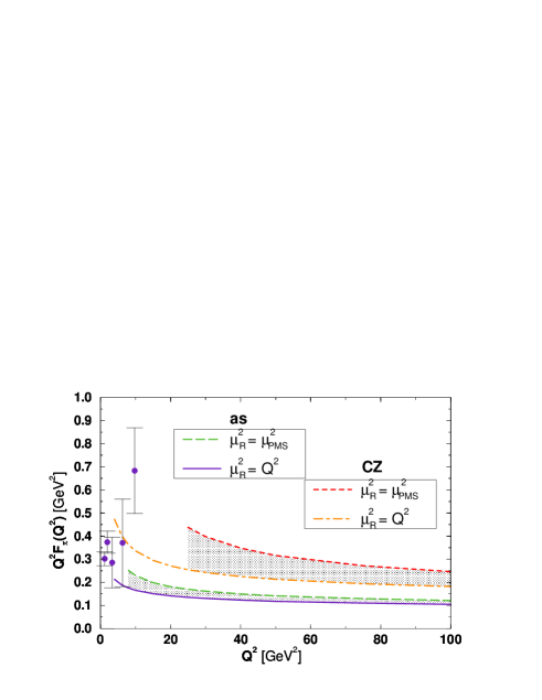
Figure 7: NLO prediction for $F_{\pi}(Q^{2})$. The shaded area denotes the range of the total NLO prediction and offers the way to asses the theoretical uncertainty.

We comment the asymptotic DA results. For $\mu_{R}^{2}=Q^{2}$ NLO corrections are rather large: the ratio (NLO correction/LO prediction) is $>30(50)\%$ until $Q^{2}>500(10)$ GeV² is reached! On the other hand, the BLM scale $\mu_{R}^{2}=(\mu_{BLM}^{2})^{as}\approx Q^{2}/106$ is very small and hence $\alpha_{S}$ is large. The $\alpha_{V}$ scheme offers the possible way out. In this scheme the scale amounts to $\mu_{R}^{2}=(\mu_{V}^{2})^{as}\approx Q^{2}/20$ ($\alpha_{S}<0.5$ and NLO corrections $<27\%$ for $Q^{2}>20$ GeV²) MNP99a .

4.3 Pion pair production

Finally, the amplitude of the process ${\gamma}{\gamma}{\rightarrow}{\pi^{+}}{\pi^{-}}$ takes the form

$${\cal M}(s,t)=\frac{\alpha_{S}(\mu_{R}^{2})}{4\pi}{\cal M}^{(1)}(s,t)+\frac{\alpha_{S}^{2}(\mu_{R}^{2})}{(4\pi)^{2}}{\cal M}^{(2)}(s,t,\mu_{R}^{2})+\cdots\,.$$ (24)

There are 20 diagrams that contribute at LO order $\gamma\gamma\rightarrow(q_{1}\bar{q_{2}})(q_{2}\bar{q_{1}})$. At NLO order 454 one-loop diagrams contribute to the NLO prediction. The existing result from the literature Nizic87 covers only the special case of the equal momenta DA, i.e., $\phi(x)=\delta(x-1/2)$. The numerical result is thus not particularly realistic. New (general) NLO calculation is in preparation and for that purpose convenient general analytical method for evaluation of one-loop Feynman integrals has been developed DuplancicN01etc .

5 NNLO prediction for the photon-to-pion transition form factor using conformal symmetry constraints

Recently, the conformal symmetry constraints were used to obtain the NNLO prediction for the photon-to-pion transition form factor MelicMP02 . The crucial ingredients of this approach lie in the fact that the massless PQCD is invariant under conformal transformations provided that the $\beta$ function vanishes, and that $F_{\pi\gamma^{*}}$ belongs to a class of two-photon processes calculable by means of the operator product expansion (OPE). One can then make use of the predictive power of the conformal OPE (COPE), the DIS results for the nonsinglet coefficient function of the polarized structure function $g_{1}$ known to NNLO order ZijlstraN94 and the explicitly calculated $\beta$-proportional NNLO terms BelitskySch98 ; MNP01 .

Let us first introduce the basic ingredients of the formalism. For the general case of the pion transition form factor ${\gamma^{*}}(q_{1})\gamma^{*}(q_{2})\rightarrow\pi(p)$ one expresses the results in terms of

$$\bar{Q}^{2}=-\frac{q_{1}^{2}+q_{2}^{2}}{2}\qquad\mbox{and}\qquad\qquad\omega=\frac{q_{1}^{2}-q_{2}^{2}}{q_{1}^{2}+q_{2}^{2}}\,.$$ (25)

It is convenient to turn the convolution formula (3) into the sum over conformal moments

$$F_{\pi\gamma^{*}}(\omega,\bar{Q}^{2})=f_{\pi}\,\sum_{j=0}^{\infty}{}^{\prime}\;T_{j}(\omega,\bar{Q}^{2},\mu_{F}^{2})\,\langle\pi|{\cal O}_{jj}(\mu_{F}^{2})|0\rangle\,.$$ (26)

Here

$$T_{j}(\omega,\bar{Q}^{2},\mu_{F}^{2})=\int_{0}^{1}\;dx\;T_{H}(\omega,x,\bar{Q}^{2},\mu_{F}^{2})\;\frac{x(1-x)}{2\sqrt{2N_{c}}N_{j}}\;C_{j}^{3/2}(2x-1)$$ (27)

is the $j$th conformal moment of the elementary hard-scattering amplitude, while

$$\phi(x,\mu_{F}^{2})=\sum_{j=0}^{\infty}{}^{\prime}\;\frac{x(1-x)}{N_{j}}C_{j}^{3/2}(2x-1)\langle\pi|{\cal O}_{jj}(\mu_{F}^{2})|0\rangle\,,$$ (28)

where ${\cal O}(\mu_{F}^{2})$ represents composite conformal operator, and $N_{j}=(j+1)(j+2)/4(2j+3)$.

For the thorough review of the conformal transformations and their applications we refer to BraunKM03 . On the quantum level conformal symmetry is broken owing to the regularization and renormalization of UV divergences: coupling constant renormalization resulting in $\beta$-proportional terms and the renormalization of composite operators. The latter represents the origin of non-diagonal NLO anomalous dimensions in $\overline{\mbox{MS}}$ scheme and can be removed by finite renormalization of the hard-scattering and distribution amplitude, i.e., by the specific choice of the factorization scheme.

First, we pose the question weather we can find a factorization scheme in which conformal symmetry holds true up to $\beta$-proportional terms? Renormalization group equation for the operators ${\cal O}$, equivalent to the DA evolution equation (6), is given by

$$\mu\frac{d}{d\mu}{\cal O}_{jl}=-\sum_{k=0}^{j}\gamma_{jk}{\cal O}_{kl}\,,$$ (29)

where the anomalous dimension matrix, corresponding to the evolution kernel (7), is given by

$$\gamma_{jk}=\frac{\alpha_{s}}{2\pi}\delta_{jk}\gamma_{j}^{(0)}+\frac{\alpha_{s}^{2}}{(2\pi)^{2}}\gamma_{jk}^{(1)}+\frac{\alpha_{s}^{3}}{(2\pi)^{3}}\gamma_{jk}^{(2)}+O(\alpha_{s}^{4})$$ (30)

with $\gamma_{j}\equiv\gamma_{jj}$. Since the conformal symmetry holds at LO, the anomalous dimensions are diagonal at LO. Similarly non-diagonal terms present in the $\overline{\mbox{MS}}$ scheme beyond LO, originate in breaking of conformal symmetry due to the renormalization of the composite operators. In contrast, the conformal subtraction (CS) scheme defined by

$${\cal O}^{\rm CS}=\hat{B}^{-1}{\cal O}^{\overline{\rm MS}},\qquad B_{jk}=\delta_{jk}+\frac{\alpha_{s}}{2\pi}B_{jk}^{(1)}+O(\alpha_{s}^{2})$$ (31)

and

$$\gamma^{\rm CS}_{jk}=\delta_{jk}\gamma_{j}+\theta(j>k)\frac{\beta}{g}\Delta_{jk}$$ (32)

preserves the conformal symmetry up to $\beta$-proportional terms.

Second, we ask weather and how can we use the predictive power of conformal symmetry? The process of interest belongs to quite a large class of two-photon processes calculable by means of OPE MullerRGDH94 . DVCS, deeply inelastic lepton–hadron scattering (DIS) and production of various hadronic final states by photon–photon fusion belong to this class of processes. Such processes can be described by a general scattering amplitude given by the time-ordered product of two-electromagnetic currents sandwiched between the hadronic states. For a specific process, the generalized Bjorken kinematics at the light-cone can be reduced to the corresponding kinematics, while the particular hadron content of the process reflects itself in the non-perturbative part of the amplitude. Hence, the generalized hard-scattering amplitude enables us to relate predictions of different two-photon processes on partonic level.

Conformal OPE (COPE) for two-photon processes works under the assumption that conformal symmetry holds (CS scheme and $\beta$=0), and the Wilson coefficients are then, up to normalization, fixed by the ones appearing in DIS structure function $g_{1}$ (calculated to NNLO order). Conformal symmetry breaking terms proportional to $\beta$ function alter COPE result. One can make use of $\beta$-proportional NNLO terms explicitly calculated in $\overline{\mbox{MS}}$ scheme BelitskySch98 ; MNP01 . We note here that there exists freedom in defining $\beta$-proportional terms in CS scheme and hence we speak of CS scheme, $\overline{\mbox{CS}}$ scheme, $\ldots$ (for detailed explanation see MelicMP02 ).

Finally we list the numerical results for the special case $\omega=\pm 1$ and $j=0$, i.e., asymptotic DA. For $\mu_{R}^{2}=2\bar{Q}^{2}$

$$F_{\pi\gamma}(\bar{Q}^{2}) = \frac{\sqrt{2}f_{\pi}}{2\bar{Q}^{2}}\left[1-\frac{\alpha_{s}{(2\bar{Q}^{2})}}{\pi}-\left\{{7.23\atop 5.14}\right\}\frac{\alpha_{s}^{2}{(2\bar{Q}^{2})}}{\pi^{2}}\right.$$ (34)

$$\left.+O(\alpha_{s}^{3})\right]\quad\mbox{in}\quad\left\{{\mbox{CS}\atop\overline{\mbox{CS}}}\right.\;\mbox{-scheme}\,,$$

while for the BLM prescription $\mu_{R}^{2}=\mu_{\rm BLM}^{2}$

$$F_{\pi\gamma}(\bar{Q}^{2})=\frac{\sqrt{2}f_{\pi}}{2\bar{Q}^{2}}\left[1-\,\frac{\alpha_{s}{(\mu_{\rm BLM}^{2})}}{\pi}+0.92\frac{\alpha_{s}^{2}{(\mu_{\rm BLM}^{2})}}{\pi^{2}}+O(\alpha_{s}^{3})\right]\,.$$ (35)

Here

$$\mu_{\rm BLM}^{2}=2Q^{2}\left\{{1/37.43\atop 1/14.78}\right\}\quad\mbox{in}\quad\left\{{\mbox{CS}\atop\overline{\mbox{CS}}}\right.\mbox{-scheme}\,.$$ (36)

One notices that, similarly to the pion electromagnetic form factor results presented in the preceding section, for $\mu_{R}^{2}$ equal to the characteristic scale of the process the QCD corrections are large , while for the BLM scale these corrections are smaller but the scale itself is also rather small leading to large expansion parameter $\alpha_{S}$. The $\alpha_{V}$ scheme could as in the case of the pion electromagnetic form factor offer the way out and physically better motivated description of the transition form factor.

We mention, that, as already noticed in DiehlKV01 and shown in MelicMP02 , the significance of higher-conformal moments decreases with $|\omega|$ and that with decreasing $|\omega|$ the difference between various schemes also decreases. Hence, small $|\omega|$ region is suitable for a novel test of PQCD.

6 Conclusions

Although the higher-order QCD corrections are important, only few exclusive processes have been explicitly calculated to NLO order. The inclusion of higher-order corrections stabilizes the dependence on renormalization scale. Still, the usual choice $\mu_{R}^{2}=[\mbox{characteristic scale of the process}]$ leads to large corrections. Other choices of scales (BLM, $\alpha_{V}$ scheme) are preferable and more physical. More effort in calculating higher-order corrections are needed and some tools applicable to the kinematic region of interest are underway. Furthermore, for some processes (example: NNLO calculation of photon-to-pion transition form factor), one can make use of the predictive power of conformal symmetry to avoid cumbersome higher-order calculations.

References

- (1) G. P. Lepage and S. J. Brodsky: Phys. Lett. B 87, 359 (1979); G. P. Lepage and S. J. Brodsky: Phys. Rev. Lett. 43, 545 (1979) [Erratum-ibid. 43, 1625 (1979)]; A. V. Efremov and A. V. Radyushkin: Theor. Math. Phys. 42, 97 (1980) [Teor. Mat. Fiz. 42, 147 (1980)]; A. V. Efremov and A. V. Radyushkin: Phys. Lett. B 94, 245 (1980); A. Duncan and A. H. Mueller: Phys. Lett. B 90, 159 (1980); A. Duncan and A. H. Mueller: Phys. Rev. D 21, 1636 (1980)
- (2) G. P. Lepage and S. J. Brodsky: Phys. Rev. D 22, 2157 (1980)
- (3) R. D. Field, R. Gupta, S. Otto and L. Chang: Nucl. Phys. B186, 429 (1981)
- (4) F. M. Dittes and A. V. Radyushkin: Sov. J. Nucl. Phys. 34, 293 (1981) [Yad. Fiz. 34, 529 (1981)]
- (5) M. H. Sarmadi: Ph. D. thesis, University of Pittsburgh, 1982, UMI 83-18195
- (6) R. S. Khalmuradov and A. V. Radyushkin: Sov. J. Nucl. Phys. 42, 289 (1985) [Yad. Fiz. 42, 458 (1985)]
- (7) E. P. Kadantseva, S. V. Mikhailov and A. V. Radyushkin: Yad. Fiz. 44, 507 (1986) [Sov. J. Nucl. Phys. 44, 326 (1986)]
- (8) E. Braaten and S. Tse: Phys. Rev. D 35, 2255 (1987)
- (9) B. Melić, B. Nižić and K. Passek: Phys. Rev. D 60, 074004 (1999) [hep-ph/9802204]
- (10) F. del Aguila and M. K. Chase: Nucl. Phys. B193, 517 (1981)
- (11) E. Braaten: Phys. Rev. D 28, 524 (1983)
- (12) P. Kroll and K. Passek-Kumerički: Phys. Rev. D 67 (2003) 054017 [hep-ph/0210045];
- (13) B. Nižić: Phys. Rev. D 35, 80 (1987)
- (14) I. V. Musatov and A. V. Radyushkin: Phys. Rev. D 56, 2713 (1997) [hep-ph/9702443]
- (15) N. G. Stefanis, W. Schroers and H. C. Kim: Eur. Phys. J. C 18, 137 (2000) [hep-ph/0005218]
- (16) D. Müller, D. Robaschik, B. Geyer, F.-M. Dittes, and J. Hořejši: Fortschr. Phys. 42, 101 (1994) [hep-ph/9812448].
- (17) X. D. Ji: Phys. Rev. D 55, 7114 (1997) [hep-ph/9609381]; A. V. Radyushkin: Phys. Rev. D 56, 5524 (1997) [hep-ph/9704207].
- (18) L. Mankiewicz, G. Piller, E. Stein, M. Vanttinen and T. Weigl: Phys. Lett. B 425, 186 (1998) [hep-ph/9712251]
- (19) X. D. Ji and J. Osborne: Phys. Rev. D 58, 094018 (1998) [hep-ph/9801260]
- (20) A. V. Belitsky and D. Müller: Phys. Lett. B 417, 129 (1998) [hep-ph/9709379]
- (21) A. V. Radyushkin: Phys. Lett. B 385, 333 (1996) [hep-ph/9605431]; J. C. Collins, L. Frankfurt and M. Strikman: Phys. Rev. D 56, 2982 (1997) [hep-ph/9611433]
- (22) A. V. Belitsky and D. Müller: Phys. Lett. B 513, 349 (2001) [hep-ph/0105046]
- (23) A.V. Belitsky and A. Schäfer: Nucl. Phys. B527, 235 (1998) [hep-ph/9801252]
- (24) B. Melić, B. Nižić and K. Passek: Phys. Rev. D 65, 053020 (2002) [hep-ph/0107295]
- (25) B. Melić, D. Müller and K. Passek-Kumerički: Phys. Rev. D 68, 014013 (2003) [hep-ph/0212346]
- (26) H. W. Huang and P. Kroll, Eur. Phys. J. C17, 423 (2000), [hep-ph/0005318].
- (27) H. W. Huang, P. Kroll and T. Morii: Eur. Phys. J. C 23, 301 (2002) [Erratum-ibid. C 31, 279 (2003)] [hep-ph/0110208].
- (28) H. W. Huang and T. Morii: Phys. Rev. D 68, 014016 (2003) [hep-ph/0305132].
- (29) D. Müller: Phys. Rev. D 49, 2525 (1994); Phys. Rev. D 51, 3855 (1995) [hep-ph/9411338]
- (30) V. L. Chernyak and A. R. Zhitnitsky: Phys. Rept. 112, 173 (1984)
- (31) A. P. Bakulev, S. V. Mikhailov and N. G. Stefanis: Phys. Lett. B508, 279 (2001) [hep-ph/0103119]
- (32) B. Melić, B. Nižić and K. Passek: FizikaB 8, 327 (1999);
- (33) D. V. Shirkov and I. L. Solovtsov: Phys. Rev. Lett. 79, 1209 (1997) [hep-ph/9704333]
- (34) G. Grunberg: Phys. Lett. B 95, 70 (1980); Phys. Rev. D 29, 2315 (1984)
- (35) P. M. Stevenson: Phys. Lett. B 100, 61 (1981); Phys. Rev. D 23, 2916 (1981); Nucl. Phys. B 203, 472 (1982); Nucl. Phys. B 231, 65 (1984)
- (36) S. J. Brodsky, G. P. Lepage and P. B. Mackenzie: Phys. Rev. D 28, 228 (1983)
- (37) S. J. Brodsky and H. J. Lu, Phys. Rev. D 51, 3652 (1995) [hep-ph/9405218]
- (38) S. J. Brodsky, C. Ji, A. Pang and D. G. Robertson, Phys. Rev. D 57, 245 (1998) [hep-ph/9705221]
- (39) A. P. Bakulev, A. V. Radyushkin and N. G. Stefanis: Phys. Rev. D 62, 113001 (2000) [hep-ph/0005085]
- (40) B. Melić, B. Nižić and K. Passek: in Proc. of Joint INT/JLab Workshop, Newport News 1999, 279-286, hep-ph/9908510
- (41) G. Duplancic and B. Nizic: Eur. Phys. J. C 20, 357 (2001) [hep-ph/0006249]; Eur. Phys. J. C 24, 385 (2002) [hep-ph/0201306]; hep-ph/0303184.
- (42) E. B. Zijlstra and W. L. van Neerven: Nucl. Phys. B417,61 (1994) [Erratum-ibid. B426:245, (1994)]
- (43) V. M. Braun, G. P. Korchemsky and D. Muller: Prog. Part. Nucl. Phys. 51, 311 (2003) [hep-ph/0306057]
- (44) M. Diehl, P. Kroll, and C. Vogt: Eur. Phys. J. C22,439 (2001) [hep-ph/0108220].