Renormalizing the Schwinger-Dyson equations in the Auxiliary Field Formulation of $\lambda\phi^{4}$ Field Theory

Abstract

In this paper we study the renormalization of the Schwinger-Dyson equations that arise in the auxiliary field formulation of the O(N) $\phi^{4}$ field theory. The auxiliary field formulation allows a simple interpretation of the large-N expansion as a loop expansion of the generating functional in the auxiliary field $\chi$, once the effective action is obtained by integrating over the $\phi$ fields. Our all orders result is then used to obtain finite renormalized Schwinger-Dyson equations based on truncation expansions which utilize the two-particle irreducible (2-PI) generating function formalism. We first do an all orders renormalization of the two- and three-point function equations in the vacuum sector. This result is then used to obtain explicitly finite and renormalization constant independent self-consistent S-D equations valid to order 1/N, in both 2+1 and 3+1 dimensions. We compare the results for the real and imaginary parts of the renormalized Green’s functions with the related sunset approximation to the 2-PI equations discussed by Van Hees and Knoll, and comment on the importance of the Landau pole effect.

I Introduction

Recently there has been interest in studying field theory using two-particle irreducible (2-PI) methods ref:2PI in both finite temperature ref:temp ; ref:VanHees ; ref:sunset and non-equilibrium situations ref:Hu ; ref:noneq1 ; ref:noneq2 ; berges-2PI ; 4d_1 ; 4d_2 ; 3d_1 ; baacke ; juchem ; aarts . The value of the 2-PI formalism for non-equilibrium problems is that it allows one to make approximations that go beyond the Hartree or large-N approximation without encountering the serious problems of secularity found in a straightforward expansion about the Hartree or leading-order large-N approximation using the generating functional or, equivalently, the one-particle irreducible (1-PI) action ref:sec . The 2-PI methods lead to self-consistent equations for the Green’s functions which require non-perturbative renormalization. Recently the renormalization of the equations obtained from the 2-PI approach applied to the standard formulation of $\phi^{4}$ field theory (first discussed by Calzetta and Hu ref:Calzetta ) has been considered by both Van Hees and Knoll ref:VanHees ; ref:sunset , and by Blaizot et. al. ref:Blaizot . This direct loop expansion of $\phi^{4}$ field theory is a summation of the coupling constant expansion and needs to be resummed in order to be related to a 1/N expansion ref:noneq2 . The approach to renormalization in the above works was based on formal Bogoliubov-Parasiuk-Hepp-Zimmermann (BPHZ) ref:BPHZ and dimensional regularization dreg methods, rather than multiplicative renormalization bd2 ; Haymaker1 . The advantage of the multiplicative renormalization approach for initial-value problems is that it lends itself more easily to the momentum space cutoffs that occur when one uses numerical methods to solve the integro-differential equations of the closed time path (CTP) formalism CTP . In non-equilibrium situations, the Green’s function equations are usually only spatially translational invariant and to make the calculational tractable, a maximum 3-momentum is introduced (3-momentum cut-off $\Lambda$). In dynamical situations the calculational schemes that have been used usually rely on mode expansions for the quantum fields which introduce non-covariant momentum cutoffs. Therefore, for practical reasons it is useful to consider direct renormalization of the Schwinger-Dyson (S-D) equations that are rendered finite by momentum space cutoffs. Such an approach was very useful in the leading order in large-N approximation, where we found that using lattice versions of the renormalization scheme gave us results (as long as we were far from the Landau pole) that became independent of the cutoff for a wide range of cutoffs when we kept renormalized parameters fixed CHKMPA ; dcc . It was also important when studying the time evolution of the (expectation value of the) energy-momentum tensor to understand the non-covariant nature of the cutoff scheme, so that the correct physical energy densities and pressures could be extracted from the (non-covariant) situation arising in the truncation scheme used for numerical simulation ref:tmunu . By not automatically subtracting off the logarithmical ($\log$) divergences related to coupling constant renormalization, we were able to have another check on the numerical simulations by studying how the simulations became independent of the cutoff for fixed renormalized parameters.

In any truncation scheme, such as expanding the 2-PI generating functional in terms of loops or 1/N, the renormalization has to be guided by the structure of the exact renormalized S-D equations. Thus as a preliminary step to renormalizing the truncated S-D equations, one needs to know the structure of the exact renormalized S-D equations. The strategy for obtaining the renormalized S-D equations and then using them to renormalize the next to leading order in 1/N is discussed in Haymaker1 ; CHKMPA . In those papers, however, the perturbative 1/N expansion was discussed and not the resummed 1/N expansion obtained from the 2-PI formalism.

Our procedure is as follows: First we derive the exact S-D equations for the auxiliary field formalism. These S-D equations are simpler than those of the original formulation of $\phi^{4}$ field theory because the only quantities that need renormalization are the propagators for the field $\phi$ and the auxiliary field $\chi$, as well as the three-particle $\chi\phi\phi$ irreducible vertex. Analyzing graphs one finds that once those quantities are renormalized one never generates a new divergence in the coupling of four $\phi$ particles. In the cutoff S-D approach to renormalization, one has to show not only that the renormalized equations are finite, but also that they are independent of all the (infinite) renormalization constants. That is, all the equations need to be written in terms of the renormalized Green’s functions, vertices and masses. The reason for using the auxiliary field formulation of $\lambda\phi^{4}$ field theory is that the 1/N expansion has a simple interpretation as a loop expansion [in the auxiliary field] of the generating functional of the effective action obtained by integrating out the scalar fields keeping $\chi$ constant on1 ; root . The S-D equations arising from this auxiliary field formulation was first discussed in Ref. bcg .

The 1/N expansion is an asymmetric expansion which treats the $\phi$ field exactly (with $\chi$ fixed), and then counts loops in $\chi$. Thus the 2-PI formalism, which treats $\phi$ and $\chi$ on an equal footing, is not a natural formalism for incorporating the large-N approximation except in leading order. Its main virtue is that it leads to self-consistent approximations that are energy conserving and non-secular when applied in non-equilibrium contexts. The basic propagators that occur in the large-N expansion, when viewed as propagators coming from the effective Lagrangian obtained after integrating out the $\phi$ field in the path integral, have different behavior with regard to 1/N berges-2PI : the $\phi\phi$ propagator $G$ being $\mathcal{O}(1)$, the $\chi\chi$ propagator $D$ being of order 1/N and the $\chi\phi$ mixed propagator $K$ (which vanishes if symmetry is unbroken) is also of order 1/N. Thus the first nontrivial two-loop 2-PI vacuum graph has terms $GGD\sim$ 1/N and $KKG\sim$ 1/N². At the level of the equation for the inverse two-point Green’s functions, the first nontrivial approximation (counting loops) has no vertex corrections, but mixes orders of 1/N. Two approximations which have been studied recently in studies of thermalization have been based on keeping one or both of these two-loop graphs ref:noneq1 ; ref:noneq2 . The first approximation has been called the 2-PI 1/N expansion and the second the bare-vertex approximation (BVA). Both these approximations are identical when $\langle\phi\rangle=0$ and thus the renormalization scheme is identical for both approximations. We find that both approximations after renormalization require that the renormalized vertex function is set to 1. Thus the BVA is a misnomer in dimensions greater than $2+1$ where wave function and vertex function renormalizations are necessary.

Recently, the 2-PI 1/N expansion has been used to study the nonequilibrium dynamics of field theory in 3+1 dimensions: First, in Ref. 4d_1 , the 2-PI 1/N was used to study the parametric resonance of an O(N) symmetric scalar theory, at very weak coupling constant. Secondly, in Ref 4d_2 , the same approximation was used to investigate the nonequilibrium dynamics of a 3+1 dimensional theory with Dirac fermions coupled to scalars via a chirally invariant Yukawa interaction. In the later case, the system was shown to reach, at late times, a state which was well described by a thermal distribution. In the above work, only the quadratic mass divergences were eliminated, and the renormalized mass extracted from the oscillation frequency. Determining the renormalized mass dynamically makes it a bit more difficult to study the behavior of the theory for fixed renormalized mass as a function of the momentum space cutoff. The advantage of having renormalized S-D equations which depend on a given fixed renormalized mass is two-fold. In the static case it allows for a rapidly convergent iteration method, since the influence of cuts on the Green’s function start only at $p^{2}=9m^{2}$, where $m$ is the physical mass. Secondly, in the time evolution problem, the range of cutoffs which lead to results insensitive to the cutoff and the Landau pole value can be easily explored. Another recent development is the use of the 2-PI methods to obtain universal behavior at a critical point 3d_1 , where encouraging results for critical indices have been obtained.

The S-D equations we investigate here were studied earlier by Bender, Cooper and Guralnik bcg ; CHKMPA and are similar in structure to those obtained for the Gross-Neveu model and analyzed at all orders by Haymaker, Cooper et al. Haymaker1 . Our approach to the renormalization of the S-D equations parallels the treatment in that body of work and allows a simple renormalization scheme at order 1/N where the renormalized vertex is replaced by $1$.

We organize this paper as follows. In Section II we introduce the auxiliary field formalism and discuss the 1/N expansion as well as derive the unrenormalized S-D equations for the two- and three-point functions. We also discuss 2-PI expansion and the BVA. In Section III we discuss the renormalization of the vacuum sector of the unbroken theory. In Section IV we display the self-consistent renormalized S-D equations for the vacuum sector valid to order 1/N. We solve these equations in the vacuum sector by an iteration scheme based on utilizing the lowest order in 1/N results and dispersion relations using a scheme used in Ref. ref:sunset . We compare our results to the related sunset approximation discussed in Ref. ref:sunset and find that at large coupling constant, $g$, there are significant differences between the sunset approximation and the next-to-leading order in $1/N$ self-consistent approximation. Finally, in Section V, we comment on the effect of the Landau Pole (triviality of continuum $\lambda\phi^{4}$ field theory phi4 ) on our treatment of the 3+1 dimensional problem.

II Auxiliary Field Formulation of the O(N) model

Consider the Lagrangian for O(N) symmetry:

$$\mathcal{L}[\phi,\partial_{\mu}\phi]\ =\ \frac{1}{2}\,\Bigl{[}\partial_{\mu}\phi_{i}(x)\,\partial^{\mu}\phi_{i}(x)+\mu^{2}\,\phi_{i}^{2}(x)\Bigr{]}$$

$$-\frac{g}{8}\,[\phi_{i}^{2}(x)]^{2}-\frac{\mu^{4}}{2g}\>.$$ (1)

Here, $g$ denotes the scaled coupling constant $g=\lambda/N$. The Einstein summation convention for repeated indices is implied throughout this paper.

We introduce a composite field $\chi(x)$ by adding to the Lagrangian a term

$$+\ \frac{1}{2g}\,\left\{\chi(x)-\frac{g}{2}\,\Bigl{[}\,\phi_{i}^{2}(x)-\frac{2\mu^{2}}{g}\,\Bigr{]}\right\}^{2}\>.$$ (2)

This gives a Lagrangian of the form

$$\mathcal{L}[\phi,\chi,\partial_{\mu}\phi]\ =\ \frac{1}{2}\,\Bigl{[}\partial_{\mu}\phi_{i}(x)\,\partial^{\mu}\phi_{i}(x)-\chi(x)\,\phi_{i}^{2}(x)\Bigr{]}$$

$$+\frac{\mu^{2}\,\chi(x)}{g}+\frac{\chi^{2}(x)}{2\,g}\>,$$ (3)

which leads to the classical equations of motion

$$\Bigl{[}\Box+\chi(x)\Bigr{]}\,\phi_{i}(x)=0\>,$$ (4)

and the constraint (“gap”) equation

$$\chi(x)=-\mu^{2}+\frac{g}{2}\,\sum_{i}\,\phi_{i}^{2}(x)\>.$$ (5)

II.1 The Large-N expansion

The generating functional for the graphs of the auxiliary field formalism is given by

$$Z[j_{i},K]\ =\ \exp(i\,N\,W[j,K])$$ (6)

$$\ =\ \int\mathrm{d}\chi\prod_{i=1}^{N}\mathrm{d}\phi_{i}\exp\biggl{\{}i\int\mathrm{d}x\Bigl{[}\mathcal{L}+j_{i}(x)\phi_{i}(x)$$

$$\qquad\qquad+iNK(x)\chi(x)\Bigr{]}\biggr{\}}\>.$$

The large-N expansion is obtained by integrating the Gaussian path integrals for $\phi_{i}$, letting each $j_{i}=j$, and setting the free inverse propagator $G_{0\,ij}=\delta_{ij}\,G_{0}$ (see on1 ; root ; bcg ; CHKMPA ). This results in an effective action

$$S_{eff}[\chi;j,K]/N= \int\mathrm{d}x\,\Bigl{[}\frac{\mu^{2}\,\chi(x)}{\lambda}+\frac{\chi^{2}(x)}{2\,\lambda}+K(x)\chi(x)\Bigr{]}$$

$$+\frac{1}{2}\ j\circ G\circ j+\frac{i}{2}\ {\rm Tr}\ln G_{0}^{-1}[\chi]\>,$$ (7)

where

$$G_{0}^{-1}[\chi](x-y]\ =\ \Bigl{[}\Box+\chi(x)\Bigr{]}\,\delta(x-y)\>,$$ (8)

and we have introduced the notation

$$\int\mathrm{d}x\int\mathrm{d}y\ j_{i}(x)\ G[\chi]_{ij}(x,y)\ j_{j}(y)=N\ j\circ G\circ j\>.$$ (9)

The evaluation of the remaining path integral for $\chi$ by steepest descent then leads to the 1/N expansion. The stationary phase-point of the integrand $\chi_{s}[j,K]$ is determined (implicitly) by the relation,

$$K(x)+\biggl{\{} {\frac{1}{\lambda}}\,\Bigl{[}\chi(x)+\mu^{2}\Bigr{]}-\frac{1}{2}\ j\circ G(\ ,x)G(x,\ )\circ j$$

$$+\frac{i}{2}\ G_{0}(x,x)\biggr{\}}_{\chi=\chi_{s}}=0\>.$$ (10)

Keeping only the Gaussian fluctuations we obtain for the $W$

$$W[j,K]\equiv W^{(0)}+{\frac{1}{N}}W^{(1)}$$ (11)

$$= \frac{1}{\lambda}\chi_{s}\circ(\frac{\chi_{s}}{2}+\mu^{2})+K\circ\chi_{s}+{\frac{1}{2}}\,j\circ G_{0}[\chi_{s}]\circ j$$

$$+{\frac{i}{2}}\,{\rm Tr}\ln G_{0}^{-1}[\chi_{s}]+{\frac{i}{2N}}\,{\rm Tr}\ln D_{0}^{-1}[j,K]$$

where $\chi_{s}$ is to be viewed as a function of the sources $j$ and $K$ through Eq. (10) above, and order 1/N² terms have been dropped. The bare inverse propagator for the auxiliary field $\chi$, $D_{0}$, is defined as the second derivative of the effective action with respect to $\chi$ at the stationary phase point and its value is:

$$D^{-1}[j,K](x,y)\equiv -\frac{1}{g}\,\delta^{4}(x,y)$$ (12)

$$-N\ \Bigl{[}j\circ G_{0}(\ ,x)G_{0}(x,y)G_{0}(y,\ )\circ j$$

$$\qquad\qquad-\frac{i}{2}\,G_{0}(x,y)G_{0}(y,x)\Bigr{]}_{\chi=\chi_{s}}\>.$$

The perturbative 1/N expansion for the connected Green’s functions is obtained by treating all terms beyond the Gaussian term in the effective action perturbatively and is equivalent to a loop expansion in $\chi$ for the effective action. Unfortunately this expansion has the same defect as ordinary perturbation theory when applied to time evolution problems in that it displays secular behavior as demonstrated in ref:sec beyond the leading order in large-N. It is precisely for this reason that the 2-PI approach has proven so useful, since it leads to self-consistent S-D equation approximations that seem to be free from secularity.

For completeness, we note that the generating functional for the 1-PI graphs, which is usually called the effective action, is the Legendre transform of $W[j,K]$ to the new variables which are the expectation value of the fields $\phi={\delta W}/{\delta j}$, and $\chi={\delta W}/{\delta K}$. That is

$$\Gamma[\phi,\chi]/N\equiv W-j\circ\phi-K\circ\chi,$$ (13)

To order 1/N one obtains

$$\Gamma[\phi,\chi]/N=S_{cl}[\phi,\chi]+{\frac{i}{2}}{\rm Tr}\ln G_{0}^{-1}[\chi]+{\frac{i}{2N}}{\rm Tr}\ln D_{0}^{-1}[\phi\chi]\>,$$ (14)

where

$$D_{0}^{-1}[\phi,\chi](x,y)= -\frac{1}{g}\ \delta^{4}(x,y)-N\,\phi(x)G_{0}[\chi](x,y)\phi(y)$$

$$+{\frac{iN}{2}}\,G_{0}[\chi](x,y)G[\chi](y,x)\>.$$ (15)

II.2 The S-D equations

The S-D equations in the auxiliary field formulation treats the fields $\phi$ and $\chi$ and their two-point correlation functions on an equal basis. Thus for considering the S-D equations or the 2-PI effective action, it is useful to use the extended field and extended current notations,

$$\phi_{\alpha}(x) =[\chi(x),\phi_{1}(x),\phi_{2}(x),\ldots,\phi_{N}(x)]\>,$$ (16)

$$j_{\alpha}(x) =[J(x),j_{1}(x),j_{2}(x),\ldots,j_{N}(x)]\>,\ \alpha=0,1,\ldots,N\>,$$

where $J(x)=NK(x)$, the source of field $\chi$ introduced in the context of the large-N expansion. The generating functional $Z[j]$ and connected Green’s function generator $W[j]$ is given by the path integral:

$$Z[j]=e^{i\,W[j]}=\prod_{\alpha=0}^{N}\int\mathrm{d}\phi_{\alpha}\,e^{i\,S[\phi;j]}.$$ (17)

The path integral needs to be supplemented by stating the boundary conditions on the Green’s functions. For initial-value problems one needs the CTP boundary conditions CTP where in the time integration the time contour is a closed time path contour. However in discussing renormalization we only need to consider the vacuum equations and the Feynman boundary conditions on the fields. This is achieved by the usual $i\epsilon$ prescription in deforming time slightly into the Euclidean region. The action $S[\phi;j]$ is given by:

$$S[\phi;j]= -\frac{1}{2}\int\mathrm{d}x\!\!\int\mathrm{d}x^{\prime}\,\phi_{\alpha}(x)\,\Delta_{\alpha\beta}^{-1}[\phi](x,x^{\prime})\,\phi_{\beta}(x^{\prime})$$

$$+\int\mathrm{d}x\,\phi_{\alpha}(x)\,j_{\alpha}(x)\>.$$ (18)

Here, we have introduced the notation

$$\Delta_{\alpha\beta}^{-1}[\phi](x,x^{\prime})=\begin{pmatrix}D_{0}^{-1}(x,x^{\prime})&0\\ 0&G_{0\,ij}^{-1}(x,x^{\prime})\end{pmatrix}\>,$$ (19)

with

$$D_{0}^{-1}(x,x^{\prime}) =-\,\frac{1}{g}\ \delta(x,x^{\prime})\>,$$

$$G_{0\,ij}^{-1}(x,x^{\prime}) =\Bigl{[}\Box+\chi(x)\Bigr{]}\,\delta_{ij}\delta(x,x^{\prime})\>.$$ (20)

The above are the diagonal entries in the Green’s function matrix $G^{-1}_{0\,\alpha\beta}[\phi](x,x^{\prime})$ defined as follows:

$$G_{0\,\alpha\beta}^{-1}[\phi](x,x^{\prime})= -\frac{\delta^{2}S[\phi;j]}{\delta\phi_{\alpha}(x)\,\delta\phi_{\beta}(x^{\prime})}$$ (21)

$$= \begin{pmatrix}D_{0}^{-1}(x,x^{\prime})&\bar{K}_{0\,j}^{-1}(x,x^{\prime})\\ K_{0\,i}^{-1}(x,x^{\prime})&G_{0\,ij}^{-1}(x,x^{\prime})\end{pmatrix}\>,$$

while the off-diagonal elements are

$$K_{0\,i}^{-1}[\phi](x,x^{\prime})\ =\ \bar{K}_{0\,i}^{-1}[\phi](x,x^{\prime})\ =\ \phi_{i}(x)\,\delta(x,x^{\prime})\>.$$ (22)

The S-D equations are obtained from the identity

$$\prod_{\beta=0}^{N}\int\mathrm{d}\phi_{\beta}\ \frac{\delta}{\delta\phi_{\alpha}(x)}\ e^{i\,S[\phi;j]}\ =\ 0\>.$$ (23)

The Heisenberg equations of motion and constraint describing the time evolution of the O(N) model are obtained as

$$-\frac{1}{g}\,\chi(x)+\frac{1}{2}\sum_{i}\ \Bigl{[}\phi_{i}^{2}(x)+G_{ii}(x,x)/i\Bigr{]}-\frac{\mu^{2}}{g}=J(x)\>,$$ (24)

$$\Bigl{[}\Box+\chi(x)\Bigr{]}\,\phi_{i}(x)+K_{i}(x,x)/i=j_{i}(x)\>.$$ (25)

where the Green’s functions $G_{\alpha\beta}[j](x,x^{\prime})$ are defined by:

$$G_{\alpha\beta}[j](x,x^{\prime})= \frac{\delta\phi_{\alpha}(x)}{\delta j_{\beta}(x^{\prime})}=\frac{\delta^{2}W[j]}{\delta j_{\alpha}(x)\,\delta j_{\beta}(x^{\prime})}$$ (26)

$$= \begin{pmatrix}D(x,x^{\prime})&K_{j}(x,x^{\prime})\\ \bar{K}_{i}(x,x^{\prime})&G_{ij}(x,x^{\prime})\end{pmatrix}\>.$$

Next, we introduce the 1-PI generating functional or effective action $\Gamma[\phi]$ by performing the Legendre transformation

$$\Gamma[\phi]=W[j]-\int\mathrm{d}x\,\phi_{\alpha}(x)j_{\alpha}(x)\>.$$ (27)

We obtain the equations of motion and constraint

$$-\frac{\delta\Gamma[\phi]}{\delta\chi(x)} =J(x)$$ (28)

$$=-\frac{1}{g}\,\chi(x)+\frac{1}{2}\sum_{i}\Bigl{[}\phi_{i}^{2}(x)+G_{ii}(x,x)/i\Bigr{]}-\frac{\mu^{2}}{g}\>,$$

$$-\frac{\delta\Gamma[\phi]}{\delta\phi_{i}(x)} =j_{i}(x)$$ (29)

$$=\Bigl{[}\Box+\chi(x)\Bigr{]}\,\phi_{i}(x)+K_{i}(x,x)/i\>.$$

We also define the inverse Green’s functions

$$G_{\alpha\beta}^{-1}[\phi](x,x^{\prime})= \frac{\delta j_{\alpha}(x)}{\delta\phi_{\beta}(x^{\prime})}=-\frac{\delta^{2}\Gamma[\phi]}{\delta\phi_{\alpha}(x)\,\delta\phi_{\beta}(x^{\prime})}$$ (30)

$$= \begin{pmatrix}D^{-1}(x,x^{\prime})&\bar{K}_{j}^{-1}(x,x^{\prime})\\ K_{i}^{-1}(x,x^{\prime})&G_{ij}^{-1}(x,x^{\prime})\end{pmatrix}\>,$$

such that

$$\int\mathrm{d}x^{\prime\prime}G_{\alpha\beta}^{-1}[\phi](x,x^{\prime\prime})\,G_{\beta\gamma}[j](x^{\prime\prime},x^{\prime})=\delta_{\alpha\gamma}\delta(x,x^{\prime})\>.$$ (31)

The Green’s functions $G_{\alpha\beta}$ are obtained by inverting the equation

$$G_{\alpha\beta}^{-1}(x,x^{\prime})=G_{0\,\alpha\beta}^{-1}(x,x^{\prime})+\Sigma_{\alpha\beta}(x,x^{\prime})\>,$$ (32)

where $G_{0\,\alpha\beta}^{-1}(x,x^{\prime})$ is given by Eq. (21), and we have introduced the generalized self-energy matrix $\Sigma_{\alpha\beta}(x,x^{\prime})$ as

$$\Sigma_{\alpha\beta}[\phi](x,x^{\prime})=\begin{pmatrix}\Pi(x,x^{\prime})&\Omega_{j}(x,x^{\prime})\\ \bar{\Omega}_{i}(x,x^{\prime})&\Sigma_{ij}(x,x^{\prime})\end{pmatrix}\>.$$ (33)

By definition, the elements of the self-energy matrix are given as

$$\Sigma_{00}\ \rightarrow\ \Pi(x,x^{\prime}) =\frac{1}{2i}\,\frac{\delta G_{jj}(x^{\prime},x^{\prime})}{\delta\chi(x)}\>,$$ (34)

$$\Sigma_{i0}\ \rightarrow\ \bar{\Omega}_{i}(x,x^{\prime}) =\frac{1}{2i}\,\frac{\delta G_{jj}(x^{\prime},x^{\prime})}{\delta\phi_{i}(x)}\>,$$

$$\Sigma_{0j}\ \rightarrow\ \Omega_{j}(x,x^{\prime}) =\frac{1}{i}\,\frac{\delta K_{j}(x^{\prime},x^{\prime})}{\delta\chi(x)}\>,$$

$$\Sigma_{ij}\ \rightarrow\ \Sigma_{ij}(x,x^{\prime}) =\frac{1}{i}\,\frac{\delta K_{j}(x^{\prime},x^{\prime})}{\delta\phi_{i}(x)}\>.$$

The elements of the self-energy matrix are obtained by taking the functional derivative of Eq. (31). We have

$$\frac{\delta G_{\alpha\beta}[j](x_{1},x_{2})}{\delta\phi_{\gamma}(x_{3})}= -\int\mathrm{d}x_{4}\int\mathrm{d}x_{5}G_{\alpha\delta}[j](x_{1},x_{4})$$ (35)

$$\times\Gamma_{\delta\epsilon\gamma}[\phi](x_{4},x_{5},x_{3})G_{\epsilon\beta}[j](x_{5},x_{2})\>.$$

Here, $\Gamma_{\alpha\beta\gamma}$ denotes the three-point vertex function

$$\Gamma_{\alpha\beta\gamma}[\phi](x_{1},x_{2},x_{3})= \frac{\delta G_{\alpha\beta}^{-1}[\phi](x_{1},x_{2})}{\delta\phi_{\gamma}(x_{3})}$$ (36)

$$= -\frac{\delta^{3}\Gamma[\phi]}{\delta\phi_{\alpha}(x_{1})\,\delta\phi_{\beta}(x_{2})\,\delta\phi_{\gamma}(x_{3})}\>.$$

In general, the three-point vertex function is the solution of the exact equation

$$\Gamma_{\alpha\beta\gamma}(x,x^{\prime},x^{\prime\prime})=f_{\alpha\beta\gamma}\,\delta(x,x^{\prime})\,\delta(x,x^{\prime\prime})+\frac{\delta\,\Sigma_{\alpha\beta}(x,x^{\prime})}{\delta\phi_{\gamma}(x^{\prime\prime})}\>,$$ (37)

where $f_{0,i,j}=f_{i,0,j}=f_{i,j,0}=\delta_{ij}$. The self-energy matrix depends implicitly on the three-point function as shown in Eq. (35). From this equation, one can write a S-D equation for $\Gamma$ in terms of an irreducible scattering kernel. We will derive this below in the unbroken symmetry case.

II.3 Unbroken Symmetry Case

These equations simplify considerably for the symmetric case, i.e. when $\phi(x)=0$. The Green’s function matrix is diagonal, $G_{ii}(x,x^{\prime})=G(x,x^{\prime})\,\delta_{ij}$. The self-energy matrix is also diagonal, $\Omega_{i}(x,x^{\prime})=\bar{\Omega}_{i}(x,x^{\prime})=0$, and $\Sigma_{ij}(x,x^{\prime})=\Sigma(x,x^{\prime})\,\delta_{ij}$. We have the gap equation

$$\chi(x)=-\,\mu^{2}\ +\ \frac{\lambda}{2i}\ G(x,x)\>,$$ (38)

and the Green’s functions:

$$D^{-1}(x,x^{\prime})\ =\ -\,\frac{N}{\lambda}\,\delta(x,x^{\prime})\ +\ \Pi(x,x^{\prime})\>,$$ (39)

$$G^{-1}(x,x^{\prime})\ =\ \Bigl{[}\Box+\chi(x)\Bigr{]}\,\delta(x,x^{\prime})\ +\ \Sigma(x,x^{\prime})\>,$$ (40)

where, by definition, the polarization and self-energy are

$$\Pi(x,x^{\prime}) =\frac{iN}{2}\int\!\!\mathrm{d}x_{1}\!\!\int\!\!\mathrm{d}x_{2}\,G(x,x_{1})\Gamma(x_{1},x_{2},x^{\prime\prime})G(x_{2},x^{\prime})\>,$$ (41)

$$\Sigma(x,x^{\prime}) =i\int\mathrm{d}x_{1}\!\!\!\int\mathrm{d}x_{2}D(x,x_{1})\Gamma(x_{1},x_{2},x^{\prime\prime})G(x_{2},x^{\prime})\>.$$ (42)

We notice that $\Sigma$ is of order 1/N since $D$ is of order $1/N$.

In the symmetric case, there are S-D equations for the $\chi\phi\phi$ vertex $\Gamma$ which needs renormalization: Functionally differentiating the $\phi$ inverse propagator with respect to $\chi(z)$ we can write

$$\Gamma(x,y,z)\ =\ \delta(x-y)\ \delta(x-z)$$ (43)

$$-i\int\mathrm{d}x_{1}\mathrm{d}x_{2}\mathrm{d}x_{3}G(x-x_{2})D(x-x_{1})M(x_{1},x_{2},x_{3},z)\>.$$

where $M$ is the $\phi-\chi$ 1-PI scattering amplitude in the s channel $(x_{1},x_{2})$. In this paper we will use the schematic form

$$\Gamma\ =\ 1\ -\ i\,DMG\>,$$ (44)

as shorthand for the above equation in either coordinate or momentum space when appropriate.

The three graphs contributing to this are:

$$M(x_{1}, x_{2},x_{3},x_{4})\ =\ M_{stu}(x_{1},x_{2},x_{3},x_{4})$$ (45)

$$+\int\mathrm{d}x_{5}\mathrm{d}x_{6}\Gamma(x_{2},x_{3},x_{5})D(x_{5},x_{6})\Lambda(x_{6},x_{1},x_{4})$$

$$+\int\mathrm{d}x_{5}\mathrm{d}x_{6}\Gamma(x_{1},x_{4},x_{5})G(x_{5},x_{6})\Gamma(x_{5},x_{2},x_{3})\>,$$

where

$$\Lambda(x_{1},x_{2},x_{3})=\frac{\delta D^{-1}(x_{1},x_{2})}{\delta\chi(x_{3})}$$ (46)

is the 1-PI 3-$\chi$ vertex function which is finite, and

$$M_{stu}(x_{1},x_{2},x_{3},x_{4})=\frac{\delta\Gamma(x_{1},x_{2},x_{3})}{\delta\chi(x_{4})}$$ (47)

$M_{stu}$ is the 1-PI in the s, t, and u channels scattering amplitude for $\phi-\chi$ elastic scattering. For renormalization purposes it is useful to have another representation of $\Gamma$ in terms of $K$ the $2-PI$ in the s channel scattering kernel since this will facilitate the renormalization program needed below.

II.4 BVA

In the bare-vertex approximation (BVA) ref:noneq1 , the three-point vertex function $\Gamma_{\alpha\beta\gamma}$ that appears in the S-D equations for the inverse Green’s function is approximated by keeping only the contact term, i.e.

$$\Gamma_{\alpha\beta\gamma}^{\text{(BVA)}}(x,x^{\prime},x^{\prime\prime})=f_{\alpha\beta\gamma}\,\delta(x,x^{\prime})\,\delta(x,x^{\prime\prime})\>.$$ (48)

This is justified at large-N where the vertex corrections to the inverse Green’s function equations first appear at order 1/N².

In this approximation, we have

$$\left[\frac{\delta G_{\mu\nu}(x_{1},x_{2})}{\delta\phi_{\gamma}(x)}\right]^{\text{(BVA)}}=-\ G_{\mu\alpha}(x_{1},x)f_{\alpha\beta\gamma}G_{\beta\nu}(x,x_{2})\>,$$ (49)

which leads to the self-energies $\Sigma_{\alpha\beta}^{\text{BVA}}$ given by

$$\Sigma_{00}\ \rightarrow\ \Pi^{\text{(BVA)}}(x,x^{\prime}) =\frac{i}{2}\ G_{mn}(x,x^{\prime})\ G_{mn}(x,x^{\prime})\>,$$ (50)

$$\Sigma_{i0}\ \rightarrow\ \bar{\Omega}_{i}^{\text{(BVA)}}(x,x^{\prime}) =i\,G_{im}(x,x^{\prime})\ K_{m}(x,x^{\prime})\>,$$

$$\Sigma_{0j}\ \rightarrow\ \Omega_{j}^{\text{(BVA)}}(x,x^{\prime}) =i\,\bar{K}_{m}(x,x^{\prime})\ G_{mj}(x,x^{\prime})\>,$$

$$\Sigma_{ij}\ \rightarrow\ \Sigma_{ij}^{\text{(BVA)}}(x,x^{\prime}) =i\,\Bigl{[}G_{ij}(x,x^{\prime})\ D(x,x^{\prime})$$

$$\qquad\quad+\bar{K}_{i}(x,x^{\prime})\ K_{j}(x,x^{\prime})\Bigr{]}\>,$$

where we have used the symmetry property, $G_{ij}(x,x^{\prime})=G_{ji}(x^{\prime},x)$ and $K_{i}(x,x^{\prime})=\bar{K}_{i}(x^{\prime},x)$. It can be verified by direct calculation, that indeed $\bar{\Omega}_{i}(x,x^{\prime})=\Omega_{i}(x^{\prime},x)$, as expected.

To summarize, in the BVA, one solves the equations of motion for $\phi_{i}(x)$

$$\Bigl{[}\Box+\chi(x)\Bigr{]}\,\phi_{i}(x)+K_{i}(x,x)/i=0\>,$$ (51)

and the gap equation for $\chi(x)$

$$\chi(x)=-\,\mu^{2}\ +\ \frac{g}{2}\sum_{i}\ \Bigl{[}\phi_{i}^{2}(x)+G_{ii}(x,x)/i\Bigr{]}\>,$$ (52)

self-consistently with the equations for the Green’s functions

$$G_{\alpha\beta}^{-1}(x,x^{\prime})=G_{0\,\alpha\beta}^{-1}(x,x^{\prime})+\Sigma_{\alpha\beta}^{\text{(BVA)}}(x,x^{\prime})\>.$$ (53)

In the symmetric case the BVA polarization and self-energy are simply

$$\Pi^{\text{(BVA)}}(x,x^{\prime}) =\frac{iN}{2}\,G(x,x^{\prime})\,G(x,x^{\prime})\>,$$ (54)

$$\Sigma^{\text{(BVA)}}(x,x^{\prime}) =i\,G(x,x^{\prime})\,D(x,x^{\prime})\>.$$ (55)

II.5 2-PI expansion

Here we review the 2-PI generating functional ref:2PI . We then derive the S-D equations that follow when we include in $\Gamma_{2}$ the first term in a symmetrical (in propagators $\chi\phi$) loop expansion of the generator $\Gamma_{2}$ of the 2-PI graphs, namely the two-loop graph. To obtain a 1/N reexpansion, one then recognizes that in this loop expansion, the three types of propagators have different dependence on 1/N ($G\sim\mathcal{O}(1)$ and $D,K\sim\mathcal{O}(1/N)$). The effective action is the twice-Legendre transformed generating functional:

$$\Gamma[\phi,G]\ =\ S_{\text{class}}[\phi]+\frac{i}{2}\mathrm{Tr}\{\,\ln\,[\,G^{-1}\,]\}$$ (56)

$$+\frac{i}{2}\mathrm{Tr}\{G_{0}^{-1}[\phi]\,G-1\}+\Gamma_{2}[G]\>.$$

where

$$G^{-1}_{0~{}\alpha\beta}[\phi](x,x^{\prime})=-\frac{\delta^{2}S_{\text{cl}}[\phi]}{\delta\phi_{\alpha}(x)\,\delta\phi_{\beta}(x^{\prime})}$$ (57)

For initial-value problems, $\phi$ is also a matrix in CTP space. $S_{\text{class}}$ is the classical Lagrangian written in terms of both $\phi$ and $\chi$. In the auxiliary field formalism the propagators for $\phi\phi$, $\phi\chi$ and $\chi\chi$ are treated on the same footing. Thus if we make a loop expansion the lowest order term in $\Gamma_{2}$ has two loops. In contrast, as discussed before, the 1/N approximation is asymmetric in $\chi$ and $\phi$, since it is all order in $\phi$ (for fixed $\chi$ and a loop expansion only in $\chi$.

The equations of motion for the field expectation values follow by variation of $\Gamma$ with respect to $\phi_{i}$ and $\chi$. We find

$$-\left[\square_{x}+\chi(x)\right]\phi_{i}(x)={K}_{i}(x,x),$$ (58)

and

$$\chi(x)=-\mu^{2}+\frac{g}{2}\sum_{i}[\phi_{i}^{2}(x)+G_{ii}(x,x)].$$ (59)

The equation for the two-point function follows by variation with respect to ${G}$, which gives

$${G}^{-1}_{\alpha\beta}={G}^{-1}_{0\,\alpha\beta}+\Sigma_{\alpha\beta}\>,$$ (60)

where

$$\Sigma_{\alpha\beta}\ =\ -\ 2i\ \frac{\delta\Gamma_{2}[{G}]}{\delta{G}_{\alpha\beta}}\>.$$ (61)

At the two-loop level we have that

$$\Gamma_{2}[G]\ =\ -\frac{1}{12}{\rm Tr}\{fGGGf\}$$ (62)

$$\ =\ -\frac{1}{4}\left[G_{ij}G_{ij}D+2\bar{K}_{i}K_{j}G_{ij}\right]\>.$$

Taking the derivatives of $\Gamma_{2}$ with respect to $G_{\alpha\beta}$, the $\Sigma$ matrix given by (61) leads to the same form for the matrix elements as we obtained previously from the S-D equations in the BVA. We notice, since $D\sim$ 1/N and $K\sim$ 1/N, the two contributions to $\Gamma_{2}$ are of order 1 and $1/N$, respectively, whereas the classical action is of order $N$. Thus if one is interested in counting powers of 1/N rather than loops, one would in next-to-leading order in $1/N$ ignore the second contribution to $\Gamma_{2}$. This fact distinguishes counting loops in the auxiliary field formalism from counting powers of $1/N$ as noted in Refs. ref:noneq2 ; berges-2PI .

The quantity $\Gamma_{2}[G]$ has a simple graphical interpretation in terms of all the 2-PI vacuum graphs using vertices from the interaction term $-\frac{1}{2}\chi\phi_{i}\phi_{i}$. When $\langle\phi\rangle_{0}=0$, one obtains

$$\Gamma[\chi,G_{\phi},D] \ =\ S_{\text{class}}[\chi]$$ (63)

$$+\frac{i}{2}\,\mathrm{Tr}\{\,\ln\,[\,D^{-1}\,]\}+\frac{i}{2}\,\mathrm{Tr}\{\,\ln\,[\,G_{\phi}^{-1}\,]\}$$

$$+\frac{i}{2}\,\mathrm{Tr}\{D_{0}^{-1}\,D+G_{0}^{-1}\,G_{\phi}-2\}+\Gamma_{2}[G_{\phi},D]\>.$$

where $G\equiv\{G_{\phi},D\}$ and

$$\Gamma_{2}[G_{\phi},D]=$$ (64)

$$-\frac{1}{4}\int\mathrm{d}x_{1}\int\mathrm{d}x_{2}\,D(x_{1},x_{2})\,G_{\phi}(x_{1},x_{2})\,G_{\phi}(x_{2},x_{1})\>.$$

The resulting equations for the two-point functions have no vertex corrections.

III All orders Renormalization in the Vacuum Sector

For renormalization it is necessary to only study the theory with unbroken symmetry since the renormalization is not changed when $\phi\neq 0$ (see e.g. Ref. ref:renorm ). The advantage of studying $\phi^{4}$ theory in terms of the auxiliary field $\chi$ is that the 1/N resummation improves the renormalizability as first discussed by Gross ref:Gross . The renormalized theory can then be determined in terms of two ”physical” parameters, which we will choose to be the value of the $\phi$ mass in the unbroken vacuum and value of the coupling constant at $q^{2}=0$. What we will find is that only the $\phi$ two-point function needs wave function renormalization and there is a Ward-like identity relating this renormalization constant to the $\chi\phi\phi$ vertex renormalization constant. The important effect of reexpressing $\phi^{4}$ field theory in terms of the $\chi$ propagator $D$ is that once the above renormalizations are performed, there are no further divergences in the elastic scattering of two $\phi$ particles.

III.1 Momentum space representation

Here we consider the homogeneous case, relevant to understanding the vacuum sector. In Minkowski space, we define Fourier transforms as:

$$G(x,x^{\prime})=\int[\mathrm{d}p]\,e^{-ip\cdot(x-x^{\prime})}\ G(p)\>,$$ (65)

$$D(x,x^{\prime})=\int[\mathrm{d}p]\,e^{-ip\cdot(x-x^{\prime})}\ D(p)\>,$$ (66)

where $[\mathrm{d}p]=\frac{\mathrm{d}^{d}p}{(2\pi)^{d}}$. Then, the gap equation is written as

$$\chi =-\,\mu^{2}\ +\ \frac{g}{2i}\ \int[\mathrm{d}p]\,G(p)\>,$$ (67)

and the equations for the Green’s functions as

$$D^{-1}(p)\ =\ -\,\frac{N}{\lambda}\ +\ \Pi(p)\>,$$ (68)

$$G^{-1}(p)\ =\ \bigl{[}-p^{2}+\chi\bigr{]}\ +\ \Sigma(p)\>.$$ (69)

Finally, the polarization and self-energy are given by

$$\Pi(p) =\frac{iN}{2}\int[\mathrm{d}q]\,G(q)\,\Gamma(q,p-q)\,G(p-q)\>,$$ (70)

$$\Sigma(p) ={i}\int[\mathrm{d}q]\,D(q)\,\Gamma(q,p-q)\,G(p-q)\>.$$ (71)

The only primitive vertex function for this theory is the $\chi\phi\phi$ vertex which we will just call $\Gamma=\Gamma_{ii0}$. Keeping in mind the translational invariance properties, we write

$$\Gamma(x,x^{\prime},x^{\prime\prime}) =\int[\mathrm{d}p]e^{-ip\cdot(x-x^{\prime\prime})}\!\!\int[\mathrm{d}q]e^{-iq\cdot(x^{\prime}-x^{\prime\prime})}\Gamma(p,q)\>,$$ (72)

and the vertex equation (37) becomes

$$\Gamma(p,q)\ =\ 1\ +\ \Delta\Gamma(p,q)\>.$$ (73)

The original S-D equation for $\Gamma$ can be rewritten in terms of a 2-PI scattering kernel $K_{2}$, which we schematically write in matrix form as

$$\Gamma(p,p+q)=1\ +\ i[\Gamma DK_{2}G](p,p+q)\>.$$ (74)

The primitive divergences of this theory have been discussed in detail in Ref. bcg . The minimal degree of divergence (ignoring $\log$ improvements) is given by the simple formula

$$\mathrm{D}\ =\ 4\ -\ 2\,\mathrm{B}\ -\ \mathrm{M}\>,$$ (75)

where $\mathrm{B}$ is the number of external auxiliary field propagators $D$, and $\mathrm{M}$ is the number of external meson propagator ($G$) lines. Thus the meson propagator is naively divergent as $\Lambda^{2}$ and needs two subtractions (mass and wave function renormalization), the $D$ propagator is $\log$ divergent and needs one subtraction (coupling constant renormalization), and the vertex function has D$=0$ and is $\log\ \log$ divergent. Another potentially divergent graph is the graph having four external meson lines, which in principal could be $\log$ divergent. However, the $D$ propagators actually go as $1/\ln(p^{2})$ at high momentum, and so the box graph with two D and two G propagators actually converges since

$$\int^{\Lambda}\frac{\mathrm{d}x}{x(\ln x)^{2}}\sim\frac{1}{ln\Lambda}\>.$$ (76)

In this paper all the renormalizations will take place on mass shell, and we follow the treatment in CHKMPA , since that approach is easiest to implement in the time evolution problem, with the power series in $-q^{2}+m^{2}$ becoming $\Box+m^{2}$ acting on lattice versions of $\delta$ functions. Our renormalization procedure will involve two steps. First we will identify the wave function and vertex renormalization constants as well as the physical mass of the $\phi$ particle. We will then obtain naively finite equations for the multiplicatively renormalized propagators and vertex functions. Secondly we will show that when we replace the bare vertices by the full vertex function minus a correction, we obtain finite renormalization constant free equations for the renormalized Green’s functions and vertex functions.

Before proceeding, let us define the multiplicative renormalization constants. We first identify the physical mass by the zero of the inverse propagator for the $\phi$ field,

$$G^{-1}(p^{2}=m^{2})\ =\ 0\>.$$ (77)

Once this mass is identified, then the wave function renormalization constant for $\phi$ is defined as

$$Z_{2}^{-1}(m^{2})\ =\ -\ \frac{\mathrm{d}G^{-1}(p^{2})}{\mathrm{d}p^{2}}\Bigr{|}_{p^{2}=m^{2}}\>.$$ (78)

If we write $G^{-1}=-p^{2}+\chi+\Sigma$, then we also can write Eq. (78) as

$$Z_{2}^{-1}(m^{2})\ \equiv\ 1\ -\ \frac{\mathrm{d}\Sigma(p^{2})}{\mathrm{d}p^{2}}\Bigr{|}_{p^{2}=m^{2}}\>.$$ (79)

The renormalized $\phi$ propagator is then defined by

$$G_{R}(p^{2})\ =\ Z_{2}^{-1}\ G(p^{2})\>.$$ (80)

The vertex function renormalization constant is defined by

$$\Gamma_{R}(p,p+q)\ =\ Z_{1}\ \Gamma(p,p+q)\>,$$ (81)

with the condition that on mass shell, with no momentum transfer. We have

$$\Gamma_{R}(p,p)|_{p^{2}=m^{2}}\ =\ 1\>,$$ (82)

which leads to

$$Z_{1}^{-1}\ =\ \Gamma(p,p)|_{p^{2}=m^{2}}\ \equiv\ 1\ +\ \frac{\partial\Sigma(p^{2})}{\partial\chi}\Bigr{|}_{p^{2}=m^{2}}\>.$$ (83)

We will prove later that a Ward-like identity leads to the renormalization constants being equal, i.e. $Z_{1}=Z_{2}$, which tells us that the product $\Gamma G$ is renormalization scheme invariant.

III.2 Analyzing Divergences

First let us realize that with our way of writing the Lagrangian, $D(q^{2})$ is a renormalization group (RG) invariant and is just (apart from a sign) the running renormalized coupling constant $g_{r}(q^{2})$ for scalar meson scattering via single $\chi$ meson exchange. Thus $g_{r}(0)\equiv g_{r}$ is related to the scattering at $q^{2}=0$. In weak coupling, or in leading order in large-N, $g_{r}$ is the actual value of the scattering amplitude. However, in the full theory the scattering amplitude gets corrections from all the loops involving exchanging more and more $D$ propagators. We have

$$D^{-1}(q^{2}=0)\ =\ -\,\frac{1}{g_{r}}\ =\ -\,\frac{1}{g}\ +\ \Pi(q^{2}=0)\>,$$ (84)

so that

$$-\,\frac{1}{g}\ =\ -\,\frac{1}{g_{r}}\ -\ \Pi(q^{2}=0)\>.$$ (85)

If we wish to define a coupling constant renormalization constant via

$$g=Z_{g}^{-1}g_{R}$$ (86)

then

$$Z_{g}=1+g_{R}\Pi(0)$$ (87)

In terms of $g_{R}$, the expression for the inverse propagator is

$$D^{-1}(q^{2})=-\frac{1}{g_{R}}+\Pi^{\mathrm{[sub\,1]}}(q^{2})\>,$$ (88)

with

$$\Pi^{\mathrm{[sub\,1]}}(q^{2})\ =\ \Pi(q^{2})-\Pi(0)\>.$$ (89)

Since $\Pi(q^{2})$ is naively $\log$ divergent, then $\Pi^{\mathrm{[sub\,1]}}(q^{2})$ is naively finite. At this stage we have that $\Pi=G\Gamma G$, which is not yet in a form which displays its independence of the renormalization constants.

Now let us look at the divergences of the $\phi$ propagator. If we write $G^{-1}=-p^{2}+\chi+\Sigma$, with $\Sigma=G\Gamma D$, and

$$\chi\ =\ -\ \mu^{2}\ +\ \frac{\lambda}{2i}\ G(x,x)\>,$$ (90)

then the bubble $G(x,x)$ has quadratic as well as $\log$ divergences in $3+1$, which are related to the mass and coupling constant renormalizations, respectively. In turn, the self-energy $\Sigma$ has quadratic and $\log\ \log$ divergences related to mass and wave function renormalization. Identifying the physical mass yields the relationship

$$0\ =\ -\,m^{2}\ +\ \chi\ +\ \Sigma(p^{2}=m^{2})\>.$$ (91)

To identify the naively finite part of $\Sigma$ we now expand $\Sigma$ around $p^{2}=m^{2}$

$$\Sigma(p^{2})\ \equiv\ \Sigma_{0}\ +\ \Sigma_{1}(p^{2}-m^{2})\ +\ \Sigma^{\mathrm{[sub\,2]}}(p^{2})\>,$$ (92)

where $\Sigma_{0}=\Sigma(p^{2}=m^{2})$, $\Sigma_{1}=\frac{\mathrm{d}\Sigma}{\mathrm{d}p^{2}}|_{(p^{2}=m^{2})}$, and $\Sigma^{\mathrm{[sub\,2]}}(p^{2})$ is naively finite and vanishes quadratically at the physical mass. Identifying

$$Z_{2}^{-1}(m^{2})\ \equiv\ -\frac{\mathrm{d}G^{-1}(p^{2})}{\mathrm{d}p^{2}}\Bigr{|}_{p^{2}=m^{2}}\>,$$ (93)

we can write

$$G^{-1}\ =\ Z_{2}^{-1}\left(-\,p^{2}\ +\ m^{2}\ +\ Z_{2}\Sigma^{\mathrm{[sub\,2]}}\right)\>,$$ (94)

so that

$$G_{R}^{-1}\ =\ -\,p^{2}\ +\ m^{2}\ +\ Z_{2}\Sigma^{\mathrm{[sub\,2]}}\>.$$ (95)

This equation is now naively finite but not transparently independent of the renormalization constants. We will have to symmetrize the Dyson equation for $\Sigma$ with respect to having fully dressed vertices at both ends in order to do this.

Next we study the divergence of the vertex function. The vertex function can be written as

$$\Gamma(p,q)\ =\ \Gamma(p,p)|_{p^{2}=m^{2}}\ +\ \Gamma^{\mathrm{[sub\,1]}}(p,q)\>,$$ (96)

where $\Gamma^{\mathrm{[sub\,1]}}(p,q)=\Gamma(p,q)-\Gamma(p,p)|_{p^{2}=m^{2}}$ is the vertex function once subtracted on the mass shell. Naively, the first term is $\log\ \log$ divergent, and so $\Gamma^{\mathrm{[sub\,1]}}(p,q)$ is naively finite. The renormalized vertex function on the mass shell with no momentum transfer is defined to be one, giving the equation

$$\Gamma_{R}(p,p)|_{p^{2}=m^{2}}\ =\ Z_{1}\ \Gamma(p,p)|_{p^{2}=m^{2}}\ =\ 1\>,$$ (97)

or

$$Z_{1}^{-1}\ =\ \Gamma(p,p)|_{p^{2}=m^{2}}\>.$$ (98)

From this we obtain

$$\Gamma_{R}(p,q)\ =\ Z_{1}\ \Gamma(p,q)\ =\ 1\ +\ Z_{1}\ \Gamma^{\mathrm{[sub\,1]}}(p,q)\>.$$ (99)

If we write the S-D equation for $\Gamma$ in the form $\Gamma=1+\Delta\Gamma$ then we can rewrite this as

$$\Gamma_{R}(p,q)\ =\ 1\ +\ Z_{1}\ \Delta\Gamma^{\mathrm{[sub\,1]}}(p,q)\>,$$ (100)

where the superscript means once subtracted on the mass shell. Again we need to show that the right hand side, when symmetrized appropriately, is independent of all the renormalization constants.

III.3 Obtaining finite equations for the renormalized Green’s Functions

To remove the dependence of the above equation on $Z_{1}$ and $Z_{2}$ the key ingredient is the symmetrization of the S-D equations, which usually have one bare and one full vertex function in their definition. We also need to prove the Ward-like identity that $Z_{1}=Z_{2}$, which is done as follows: We have already said that $D$ is RG invariant, so that the vacuum vertex function satisfies (for constant field $\chi$)

$$\Gamma(p,p)\ =\ \frac{\delta G^{-1}(p^{2})}{\delta\chi}\ =\ Z_{2}^{-1}\ \frac{\delta G_{R}^{-1}(p^{2})}{\delta\chi}$$

$$\ \equiv\ Z_{1}^{-1}\ \Gamma_{R}(p,p)\>.$$ (101)

However, since $\chi$ is not renormalized, we also have

$$\Gamma_{R}(p,p)\ =\ \frac{\delta G_{R}^{-1}(p^{2})}{\delta\chi}\>.$$ (102)

Thus we find that in this theory we have the identity

$$Z_{1}\ =\ Z_{2}\>.$$ (103)

This can also be shown by analyzing graphs. We have

$$Z_{1}^{-1} \ =\ \Gamma(p,p)|_{p^{2}=m^{2}}\ \equiv\ 1\ +\ \frac{\partial\Sigma(p^{2})}{\partial\chi}\Bigr{|}_{p^{2}=m^{2}}\>,$$ (104)

$$Z_{2}^{-1} \ =\ 1\ -\ \frac{\partial\Sigma(p^{2})}{\partial p^{2}}\Bigr{|}_{p^{2}=m^{2}}\>.$$ (105)

By studying graphs contributing to $Z_{1}$ and $Z_{2}$ the difference between these graphs are seen to be naively finite  bcg , and since these renormalization constants diverge as $\log\ \log\Lambda$ one has in the continuum $Z_{1}=Z_{2}$. From this identity we find that the quantity $\Gamma G$ is renormalization scheme invariant and equals $\Gamma_{R}G_{R}$. We also have, $Z_{1}\Gamma=Z_{2}\Gamma=\Gamma_{R}$.

The next step is to get an integral equation for $\Gamma$ which is iterative in $\Gamma$. The original integral equation for $\Gamma$ that one gets by functional differentiation of the equation for the inverse $\chi$ propagator is schematically

$$\Gamma\ =\ 1\ -\ i\,DMG\>,$$ (106)

where $M$ is the one 1-PI in stu $\phi\chi$ scattering amplitude defined in Eq. (45). We want to replace this equation by one in which the r.h.s also has a $\Gamma$.

First we invert Eq. (106) to obtain the formal identity (see Ref. bcg )

$$1\ =\ \Gamma\ (1\ -\ i\,DMG)^{-1}\>.$$ (107)

We can therefore introduce a $\Gamma$ into the integral equation using this identity:

$$\Gamma\ =\ 1\ +\ i\,\Gamma\ (1-iDMG)^{-1}DMG$$ (108)

$$\ \equiv\ 1\ -\ i\,\Gamma\ DK_{2}G$$

Solving for $K_{2}$ and reintroducing the coordinates, we have

$$M(x_{1},x_{2},x_{3},x_{4})\ =\ K_{2}(x_{1},x_{2},x_{3},x_{4})$$ (109)

$$\ -\ \int\ \mathrm{d}x_{5}\mathrm{d}x_{6}\mathrm{d}x_{7}\mathrm{d}x_{8}\ M(x_{1},x_{2},x_{5},x_{6})D(x_{5},x_{7})$$

$$\qquad\qquad\times\ G(x_{6},x_{8})K_{2}(x_{7},x_{8},x_{3},x_{4})\>,$$

so that $K_{2}$ is the 2-PI in the s channel irreducible kernel of the Bethe-Salpeter equation for the scattering. What is important for renormalization is that the combination $GDK$ is RG invariant as can be seen by looking at all the skeleton terms contributing to $K$. For example, if the skeleton one-particle exchange in the t channel contribution to $K$, $\Gamma G\Gamma$, is investigated, we get the combination $D\Gamma G\Gamma G$, which is obviously equal to $D_{R}\Gamma_{R}G_{R}\Gamma G_{R}$.

The key to eliminating the dependence of the renormalized Green’s function equations obtained earlier on $Z_{1}$ and $Z_{2}$ is the symmetrizing of the self-energy and polarization graphs with respect to the full vertex function. The strategy for doing this in quantum electrodynamics (QED) is found in the text book of Bjorken and Drell bd2 , where it is also shown that this procedure eliminates the problem of overlapping divergences.

We have shown we can write

$$\Gamma\ =\ 1\ -\ i\,\Gamma DK_{2}G\ =\ 1\ +\ \Delta\Gamma\>.$$ (110)

This equation allows us to substitute the bare vertex by

$$1\ =\ \Gamma-i\Gamma DK_{2}G\ \equiv\ \Gamma\ -\ \Delta\Gamma\>.$$ (111)

The right hand side now multiplicatively renormalizes exactly as $\Gamma$ does, by the above argument. Replacing bare vertices by the right hand side will exactly absorb the extra factors of $Z_{1}$ and $Z_{2}$. Equation (110) is useful to symmetrize $\Sigma$ with respect to $\Gamma$. However a different S-D equation for $\Gamma$ is needed when we symmetrize $\Pi$ which is a loop made of two $\phi$ propagators. To obtain this S-D equation we realize that we can write $D^{-1}$ as

$$D^{-1}(x_{1},x_{2})=[\Box+\chi(x_{1})]\delta(x_{1}-x_{2})+\Sigma[G,D](x_{1},x_{2})$$ (112)

where

$$\Sigma[G,D](x_{1},x_{2})=-2i\frac{\delta\Gamma_{2}[G,D]}{\delta G(x_{1},x_{2})}$$ (113)

is just a function of the exact $G$ and $D$ propagators. Thus, using the chain rule and taking the total functional derivative of $D^{-1}$ with respect to $\chi(x_{3})$, we obtain the equation

$$\Gamma(x_{1},x_{2},x_{3})=\delta(x_{1}-x_{3})\delta(x_{1}-x_{2})-\!\int\!\mathrm{d}x_{3}\mathrm{d}x_{4}\mathrm{d}x_{5}\mathrm{d}x_{6}$$

$$\times\Bigl{[}\Gamma(x_{3},x_{5},x_{6})G(x_{5},x_{3})M_{2}(x_{3},x_{4},x_{1},x_{2})G(x_{4},x_{6})$$

$$\ +\Lambda_{3}(x_{3},x_{5},x_{6})D(x_{5},x_{3})K_{2}(x_{3},x_{4},x_{1},x_{2})D(x_{4},x_{6})\Bigr{]}\>.$$ (114)

In the above we have that $\Lambda_{3}={\delta D^{-1}}/{\delta\chi}$ is the three $\chi$ 1-PI vertex function. The two scattering kernels are that $M_{2}$ is the 2-PI scattering kernel for $\phi\phi\rightarrow\phi\phi$ and $K_{2}$ here is now the t channel kernel for $\chi\chi\rightarrow\phi\phi$. Explicitly, we have

$$M_{2}(x_{1},x_{2},x_{3},x_{4}) =\frac{\delta G^{-1}(x_{1},x_{2})}{\delta G(x_{3},x_{4})}$$

$$K_{2}(x_{1},x_{2},x_{3},x_{4}) =\frac{\delta G^{-1}(x_{1},x_{2})}{\delta D(x_{3},x_{4})}\>.$$ (115)

We note that in QED, $\Lambda_{3}$ would be the three-photon vertex which is zero by Furry’s theorem furry . Again a study of graphs shows that $\Delta\Gamma$ is rendered independent of renormalization constants when multiplied by $Z_{1}=Z_{2}$. First, let us look at the Dyson equation for the renormalized vertex function. We use

$$\Gamma(p,q)\ =\ 1\ +\ \Delta\Gamma(p,q)\>,$$ (116)

where $\Delta\Gamma(p,q)=i\,[\Gamma GDK_{2}](p,q)$. Subtracting once on the mass shell leads to

$$\Gamma_{R}(p,q)\ =\ Z_{1}\Gamma(p,q)\ =\ [1+Z_{1}\Delta\Gamma^{\mathrm{[sub\,1]}}](p,q)$$

$$\ \equiv\ 1+\Delta\Gamma_{R}(p,q)\>,$$ (117)

which is now explicitly finite and free from any dependence on the renormalization constants, since

$$\Delta\Gamma_{R}(p,q)\ =\ [\Gamma_{R}G_{R}D_{R}K_{2R}]^{\mathrm{[sub\,1]}}(p,q)\>,$$ (118)

which is finite and written in terms of a renormalized skeleton expansion for the scattering kernel $K_{2R}$. Similarly using the second S-D equation we obtain

$$\Delta\Gamma_{R}(p,q)\ =\ [\Gamma_{R}G_{R}G_{R}M_{2R}]^{\mathrm{[sub\,1]}}(p,q)$$ (119)

$$+[\Lambda_{3R}D_{R}D_{R}K_{2R}]^{\mathrm{[sub\,1]}}(p,q)\>,$$

since $D_{R}\sim\mathcal{O}(1/N)$ and $\Delta\Gamma_{R}(p,q)\sim\mathcal{O}(1/N)$.

The equation for the $\chi$ propagator contains the naively finite once subtracted polarization $\Pi^{\mathrm{[sub\,1]}}=\left[G\Gamma G\right]^{\mathrm{[sub\,1]}}$. The right hand side of this equation however is not RG invariant. By inserting the second S-D equation for $\Gamma$ in the form $1=\Gamma-\Delta\Gamma$, then we have

$$\Pi^{\mathrm{[sub\,1]}}\ =\ [(\Gamma-\Delta\Gamma)GG\Gamma]^{\mathrm{[sub\,1]}}$$ (120)

$$\ \rightarrow\ [(\Gamma_{R}-\Delta\Gamma_{R})G_{R}G_{R}\Gamma_{R}]^{\mathrm{[sub\,1]}}\>,$$

and we see that all the dependence on the renormalization constants disappears.

Next let us look at the $\phi$ propagator. We have previously shown that

$$G_{R}^{-1}(p^{2})\ =\ m^{2}-p^{2}\ +\ Z_{2}\Sigma^{\mathrm{[sub\,2]}}(p^{2})\>,$$ (121)

where $\Sigma^{\mathrm{[sub\,2]}}(p^{2})$ is the twice subtracted $G\Gamma D$ and so is naively finite. So it is easy to see that once we replace the bare vertex by the first S-D equation for $\Gamma$ in the form $1=\Gamma-\Delta\Gamma$ in $\Sigma$ we again have

$$G^{-1}_{R}(q^{2})\ =\ m^{2}-p^{2}\ +\ \Sigma_{R}^{\mathrm{[sub\,2]}}(p^{2})\>,$$ (122)

with

$$\Sigma_{R}^{\mathrm{[sub\,2]}}\ =\ Z_{2}\ \Sigma^{\mathrm{[sub\,2]}}$$ (123)

$$\ =\ [(\Gamma_{R}-\Delta\Gamma_{R})G_{R}D_{R}\Gamma_{R}]^{\mathrm{[sub\,2]}}\>,$$

and the subscript referring to subtracting twice on mass shell.

III.4 Renormalizing at $q^{2}=0$

In this subsection we would like to relate the physical renormalization discussed above by conventional renormalization at the unphysical value $q^{2}=0$ which is convenient for evaluating integrals. For the inverse $\phi$ propagator we now expand $\Sigma(q^{2})$ around the point $q^{2}=0$. That is, we let

$$\Sigma(p^{2})\ \equiv\ \Sigma_{0(0)}\ +\ \Sigma_{1(0)}\ p^{2}\ +\ \Sigma_{0}^{\mathrm{[sub\,2]}}(p^{2})\>,$$ (124)

where now $\Sigma_{0(0)}=\Sigma(p^{2}=0)$, $\Sigma_{1(0)}=\frac{\mathrm{d}\Sigma}{\mathrm{d}p^{2}}|_{(p^{2}=0)}$, and $\Sigma_{0}^{\mathrm{[sub\,2]}}(p^{2})$ is again naively finite, but vanishes quadratically at $p^{2}=0$. In this case we identify

$$Z_{2(0)}^{-1}\ \equiv\ -\frac{\mathrm{d}G^{-1}(p^{2})}{\mathrm{d}p^{2}}\Bigr{|}_{p^{2}=0}\>.$$ (125)

We can write

$$G^{-1}(p^{2})\ =\ Z_{2(0)}^{-1}\left[-p^{2}+m_{0}^{2}\ +\ Z_{2(0)}\ \Sigma_{0}^{\mathrm{[sub\,2]}}(p^{2})\right]\>,$$ (126)

so that

$$G_{R}^{-1}(p^{2})\ =\ -p^{2}+m_{0}^{2}\ +\ Z_{2(0)}\ \Sigma_{0}^{\mathrm{[sub\,2]}}(p^{2})\>.$$ (127)

The same argument as before allows us to symmetrize the dependence of $\Sigma$ on the vertex function and obtain:

$$G_{R}^{-1}(p^{2})\ =\ -p^{2}+m_{0}^{2}\ +\ \Sigma_{0\,R}^{\mathrm{[sub\,2]}}(p^{2})\>.$$ (128)

The finite mass $m_{0}^{2}$ is related to the physical mass which is the zero of the renormalized Green’s function via

$$0\ =\ -m^{2}+m_{0}^{2}\ +\ \Sigma_{0\,R}^{\mathrm{[sub\,2]}}(m^{2})\>.$$ (129)

This can also be written as

$$m^{2}\ =\ Z_{2(0)}^{-1}\ m_{0}^{2}\ +\ \Sigma(m^{2})-\Sigma(0)\>.$$ (130)

For the vertex renormalization we now have

$$Z_{1(0)}^{-1}\ =\ \Gamma(p,p)|_{p^{2}=0}\ \equiv\ 1\ +\ \frac{\partial\Sigma(p^{2})}{\partial\chi}\Bigr{|}_{p^{2}=0}\>,$$ (131)

and the Ward-like identity is now $Z_{1(0)}=Z_{2(0)}$.

IV Renormalized S-D equations up to order 1/N

Now that we have an all orders renormalization procedure, to renormalize these equations at order 1/N we realize that $\Delta\Gamma$ is of order 1/N so it can be ignored in the integral equations for $\Pi$ and $\Sigma$. Thus, it is consistent with the 1/N approximation to set $\Gamma_{R}=1$. This now gives us the finite renormalized equations for the inverse Green’s functions, exact up to order 1/N. We can now write the renormalized S-D equations in the unbroken symmetry case as follows:

For the $\phi$ inverse propagator we have ($G_{ij}=G\,\delta_{ij})$:

$$G^{-1}_{R}(q^{2})\ =\ m^{2}-p^{2}\ +\ \Sigma_{R}^{\mathrm{[sub\,2]}}(p^{2})\>.$$ (132)

with

$$\Sigma_{R}(x,y)\ =\ i\,G_{R}(x,y)D_{R}(x,y)\>,$$ (133)

so that in momentum space

$$\Sigma_{R}(q^{2})\ =\ i\ \int[d^{d}p]\ G_{R}(q-p)D_{R}(p)\>.$$ (134)

We have

$$\Sigma_{R}^{\mathrm{[sub\,2]}}(p^{2})\ =\ \Sigma_{R}(p^{2})\ -\ \Sigma_{R}(p^{2}=m^{2})$$

$$\ -\ (p^{2}-m^{2})\ \Sigma_{1\,R}(p^{2}=m^{2})\>.$$ (135)

For the $\chi$ inverse propagator we have ($g_{R}=\lambda_{R}/N$)

$$D_{R}^{-1}(q^{2})\ =\ -\ g_{R}^{-1}\ +\ \Pi_{R}^{\mathrm{[sub\,1]}}(q^{2})\>,$$ (136)

where

$$\Pi_{R}^{\mathrm{[sub\,1]}}(p^{2})\ =\ \Pi_{R}(p^{2})-\Pi_{R}(0)\>,$$ (137)

and

$$\Pi_{R}(x,y)\ =\ \frac{iN}{2}\ G_{R}(x,y)G_{R}(y,x)\>,$$ (138)

or in momentum space

$$\Pi_{R}(q^{2})\ =\ \frac{iN}{2}\ \int[d^{d}p]\ G_{R}(q-p)G_{R}(p)\>.$$ (139)

In order to solve these equations, one first specifies the value of the renormalized mass, $m^{2}$, and the renormalized coupling constant, $g_{R}$. Then, both $G_{R}(p^{2})$ and $D_{R}(p^{2})$, and therefore $\Sigma_{R}(p^{2})$, are just functionals of the finite quantity $\Sigma_{R}^{\mathrm{[sub\,2]}}(p^{2})$. Then Eq. (135) is the self-consistent equation we need to solved for the $\Sigma_{R}^{\mathrm{[sub\,2]}}(p^{2})$.

One way of solving this equation at large-N is to realize that $\Sigma_{R}^{\mathrm{[sub\,2]}}$ is finite and of order 1/N so that one can start with the value of $\Sigma_{R}^{\mathrm{[sub\,2]}}$ found in leading order in the large-N approximation and iterate until convergence is obtained. The strategy for doing this in the related approximation of the keeping the three-loop sunset graph in $\Gamma_{2}$ (which is the first term in a coupling constant reexpansion of the composite field propagator $D$) is very clearly discussed in the papers of H. Van Hees and J.Knoll ref:VanHees ; ref:sunset and we will essentially repeat their strategy here. Once $\Sigma^{\mathrm{[sub\,2]}}$ is obtained, then one can reconstruct $G_{R}$ and $D_{R}$, and finally the subtraction terms $\Sigma_{R}(m^{2})$ and $\Sigma_{1R}(m^{2})$ needed for the renormalization of the time dependent evolution equations, as well as the renormalization constants $Z_{1}=Z_{2}$. If one instead renormalizes at $q^{2}=0$, one first specifies the parameters $m_{0}^{2}$ and $g_{R}$, and then gets a self-consistent equation to solve for $\Sigma_{0\,R}^{\mathrm{[sub\,2]}}(p^{2})$. Again one reconstructs the propagators, the self-energy and vacuum polarization, and determines the physical mass from the parameter $m_{0}^{2}$ using

$$m^{2}\ =\ m_{0}^{2}\ +\ \Sigma_{0\,R}^{\mathrm{[sub\,2]}}(p^{2}=m^{2})\>.$$ (140)

The advantage of the mass shell renormalization is that one definitely has a clear separation between the pole contribution to the dispersion relation for the Green’s function discussed below and the three-particle cut which starts at $9m^{2}$. This large mass for the cut then allows a rapidly converging iteration strategy for $\Sigma$ starting with the leading order in large-N propagators.

IV.1 General strategy

Assuming that indeed the Green’s functions $G_{R}(p^{2})$ and $D_{R}(p^{2})$ vanish at infinity (which is true in 3+1 dimensions, but will need to be modified in $2+1$ dimensions for $D_{R}(p)$), then we can write the spectral representations for the renormalized Green’s functions as

$$G_{R}(p^{2}) =\frac{1}{m^{2}-p^{2}+\Sigma_{R}^{\mathrm{[sub\,2]}}(p^{2})-i\epsilon}$$ (141)

$$=\int_{0}^{\infty}\frac{\mathrm{d}(m_{1}^{2})}{\pi}\frac{\mathrm{Im}G_{R}(m_{1}^{2})}{m_{1}^{2}-p^{2}-i\epsilon}\>,$$ (142)

$$D_{R}(p^{2}) =\frac{1}{-g_{R}^{-1}+\Pi_{R}^{\mathrm{[sub\,1]}}(p^{2})}$$ (143)

$$=\int_{0}^{\infty}\frac{\mathrm{d}(m^{2})}{\pi}\frac{\mathrm{Im}D_{R}(m_{2}^{2})}{m_{2}^{2}-p^{2}-i\epsilon}\>,$$ (144)

where

$$\Sigma_{R}(p^{2})\ =\ i\int[\mathrm{d}^{d}q]D_{R}(p-q)G_{R}(q)$$ (145)

$$\ =\ \int_{0}^{\infty}\frac{\mathrm{d}(m_{1}^{2})}{\pi}\mathrm{Im}D_{R}(m_{1}^{2})$$ (146)

$$\times\int_{0}^{\infty}\frac{\mathrm{d}(m_{2}^{2})}{\pi}\mathrm{Im}G_{R}(m_{2}^{2})K^{[d]}(p^{2};m_{1}^{2},m_{2}^{2})\>,$$

$$\Pi_{R}(p^{2})\ =\ \frac{i}{2}\int[\mathrm{d}^{d}q]G_{R}(p-q)G_{R}(q)$$ (147)

$$\ =\ \frac{1}{2}\int_{0}^{\infty}\frac{\mathrm{d}(m_{1}^{2})}{\pi}\mathrm{Im}G_{R}(m_{1}^{2})$$ (148)

$$\times\int_{0}^{\infty}\frac{\mathrm{d}(m_{2}^{2})}{\pi}\mathrm{Im}G_{R}(m_{2}^{2})K^{[d]}(p^{2};m_{1}^{2},m_{2}^{2})\>,$$

with

$$K^{[d]}(p^{2};m_{1}^{2},m_{2}^{2})$$

$$=i\int\frac{[\mathrm{d}^{d}q]}{(m_{1}^{2}-(p-q)^{2}-i\epsilon)(m_{2}^{2}-q^{2}-i\epsilon)}$$ (149)

$$=-\int\ \frac{[\mathrm{d}^{d}q_{E}]}{(m_{1}^{2}+(p_{E}-q_{E})^{2})(m_{2}^{2}+q_{E}^{2})}\>,$$ (150)

with $p^{2}\rightarrow-p_{E}^{2}$. The last (Euclidean) integral is found for example in Itzykson and Zuber Zuber in terms of the Feynman parametrization, as

$$K^{[d]} (p^{2};m_{1}^{2},m_{2}^{2})\ =\ -\,\frac{\Gamma(2-d/2)}{(4\pi)^{d/2}}$$ (151)

$$\times\int_{0}^{1}~{}d\alpha\left[\alpha(1-\alpha)p^{2}+\alpha m_{1}^{2}+(1-\alpha)m_{2}^{2}\right]^{d/2-2}\>.$$

The advantage of writing things this way is now clear, as the kernel can be evaluated in $d$ dimensions exactly. The finite part of $\Sigma_{R}$ can be obtained by performing the subtractions directly on the kernel at the physical mass. In 2+1 dimensions $\Sigma_{R}$ requires one subtraction corresponding to mass renormalization, and in 3+1 there are two subtractions related to both mass and wave function renormalization. $\Pi$ is finite in 2+1 dimensions and goes to zero at large momentum, which will lead to the need for using a subtracted dispersion relation for $D_{R}$ in three dimensions. In 3+1 dimensions $\Pi$ is $\log$ divergent so that one needs to subtract $\Pi$ once, which corresponds to coupling constant renormalization. These subtractions when done on the kernel $K$ then automatically lead to a finite analytic (in the cut plane) expression for the subtracted kernel, which is then used to determine $\Sigma^{\mathrm{[sub\,2]}}$ and $\Pi^{\mathrm{[sub\,1]}}$ via the spectral representation.

The above equations will be solved iteratively: We start with the free renormalized $\phi$ Feynman propagator

$$G_{0}(s=p^{2})\ =\ \frac{1}{m^{2}-s-i\epsilon}$$ (152)

$$\ =\ -\ \frac{\mathcal{P}}{s-m^{2}}\ +\ i\,\pi\ \delta(s-m^{2})\>.$$

(For convenience, we shall drop for now the subscript $R$ in denoting renormalized quantities, and we will ignore the required subtractions for the polarization and self-energy.) Equation (152), in conjunction with Eq. (147), gives

$$\Pi_{0}(s) \ =\ \frac{i}{2}\ \int\ [\mathrm{d}^{d}q]\ G_{0}[(p-q)^{2}]\ G_{0}(q^{2})$$

$$\ =\ \frac{1}{2}\ K^{[d]}(s;m^{2},m^{2})\>.$$ (153)

Using Eqs. (142) and (145) we obtain, in order,

$$D_{0}(s) \ =\ \frac{1}{-\,g_{R}^{-1}+\Pi_{0}(s)}\>,$$ (154)

$$\Sigma_{0}(s) \ =\ \int_{0}^{\infty}\ \frac{\mathrm{d}(m_{1}^{2})}{\pi}\ \mathrm{Im}\ D_{0}(m_{1}^{2})\ K^{[d]}(s;m_{1}^{2},m^{2})\>.$$ (155)

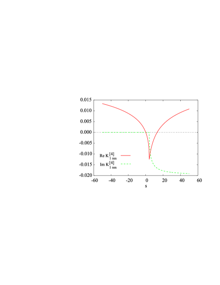
Figure 1: (Color online) $K^{[4]}_{1\,\mathrm{ren}}(s;m_{1}^{2},m_{2}^{2})$ with $m_{1}=m_{2}=m=1$.

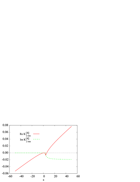
Figure 2: (Color online) $K^{[4]}_{2\,\mathrm{ren}}(s;m_{1}^{2},m_{2}^{2})$ with $m_{1}=m_{2}=m=1$.

We can now calculate the first update of the $\phi$ propagator, $G_{1}(s)$,

$$G_{1}(s) \ =\ \frac{1}{m^{2}-s+\Sigma_{0}(s)}\ =\ G_{0}(s)\ -\ \Delta G(s)\>,$$ (156)

with

$$\Delta G(s)\ =\ \frac{\Sigma_{0}(s)}{(m^{2}-s)\,[m^{2}-s+\Sigma_{0}(s)]}\>.$$ (157)

The updates of the polarization and self-energy are obtained by combining Eq. (156) with Eqs. (148) and (146). We have:

$$\Pi_{1}(s)\ =\ \Pi_{0}(s)-\int_{0}^{\infty}\frac{\mathrm{d}(m_{1}^{2})}{\pi}\,\mathrm{Im}\Delta G(m_{1}^{2})K^{[d]}(s;m_{1}^{2},m^{2})$$

$$+\frac{1}{2}\int_{0}^{\infty}\frac{\mathrm{d}(m_{1}^{2})}{\pi}\,\mathrm{Im}\Delta G(m_{1}^{2})$$ (158)

$$\qquad\times\int_{0}^{\infty}\frac{\mathrm{d}(m_{2}^{2})}{\pi}\,\mathrm{Im}\Delta G(m_{2}^{2})K^{[d]}(s;m_{1}^{2},m_{2}^{2})\>,$$

$$\Sigma_{1}(s)\ =\ \Sigma_{0}(s)-\int_{0}^{\infty}\frac{\mathrm{d}(m_{1}^{2})}{\pi}\,\mathrm{Im}D_{1}(m_{1}^{2})$$ (159)

$$\qquad\times\int_{0}^{\infty}\frac{\mathrm{d}(m_{2}^{2})}{\pi}\,\mathrm{Im}\Delta G(m_{2}^{2})K^{[d]}(s;m_{1}^{2},m_{2}^{2})\>,$$

where

$$D_{1}(p) \ =\ \frac{1}{-\,g^{-1}+\Pi_{1}(p)}\>.$$ (160)

We can now obtain the “new” correction $\Delta G(s)$, by replacing $\Sigma_{0}(s)$ with $\Sigma_{1}(s)$ in Eq. (157). Then, we iterate Eqs. (157), (158) and (159), until we achieve convergence.

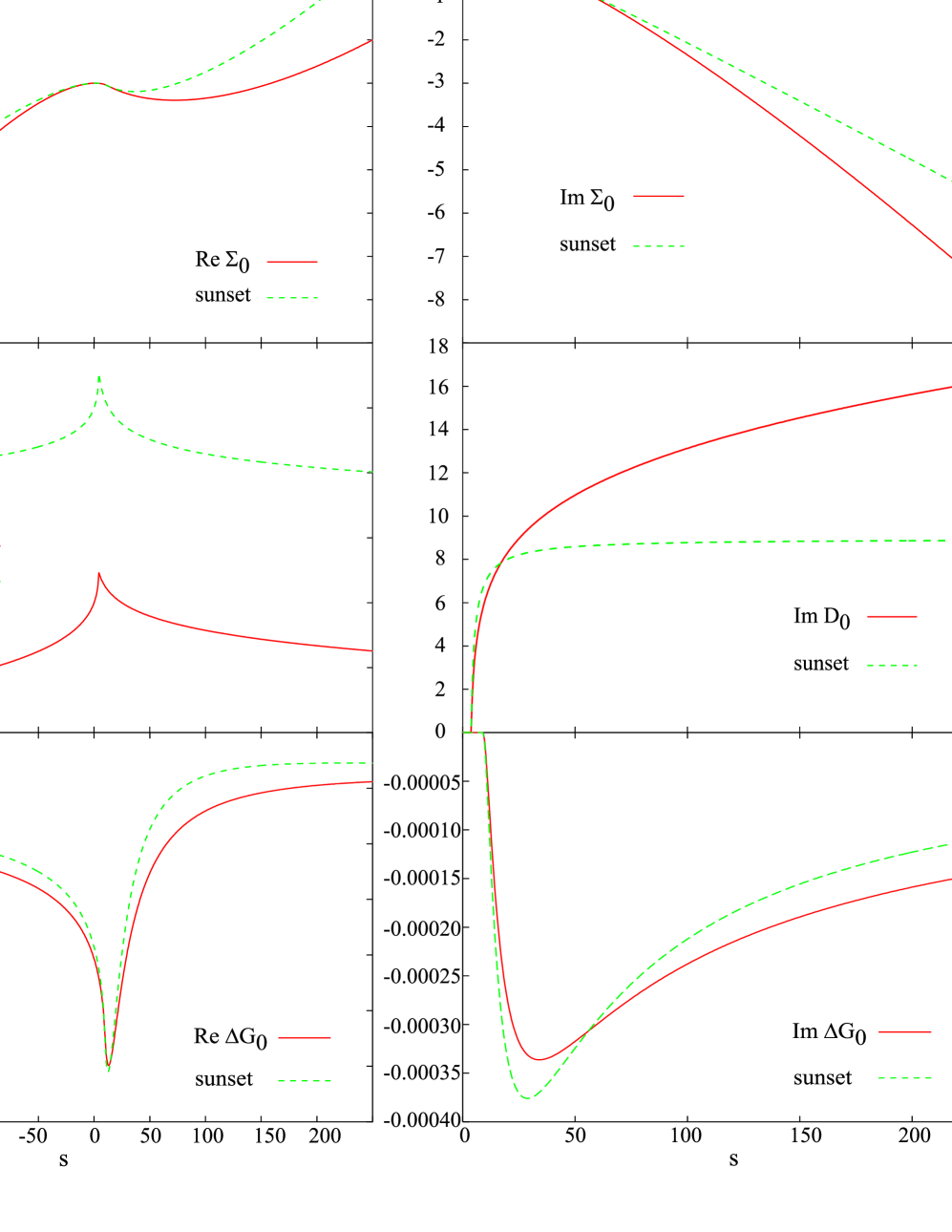
Figure 3: (Color online) First iteration results in 3+1 dimensions ($g_{R}$=30).

IV.2 3+1 dimensions

The key ingredients for this case have been previously discussed in van Hees and Knoll ref:sunset . Those authors have used dimensional regularization arguments in order to regularize the kernel

$$K^{[4]} (s=p^{2},m_{1}^{2},m_{2}^{2})\ =\$$ (161)

$$i\int[\mathrm{d}^{4}q]\frac{\mu^{2\epsilon}}{[m_{1}^{2}-(p-q)^{2}-i\epsilon](m_{2}^{2}-q^{2}-i\epsilon)}\>.$$

In the range $(m_{1}-m_{2})^{2}\leq s<(m_{1}+m_{2})^{2}$, one obtains

$$K^{[4]} (s,m_{1}^{2},m_{2}^{2})=\frac{1}{16\pi^{2}}\biggl{\{}-\frac{1}{\epsilon}+\gamma-2\ +\ \ln\Bigl{[}\frac{m_{1}m_{2}}{4\pi\mu^{2}}\Bigr{]}$$

$$+\ \frac{m_{1}^{2}-m_{2}^{2}}{s}\ \ln\Bigl{[}\frac{m_{1}}{m_{2}}\Bigr{]}\ +\ \frac{\bar{\lambda}(s,m_{1}^{2},m_{2}^{2})}{s}$$

$$\quad\times\biggl{[}\tan^{-1}\Bigl{[}\frac{m_{+}m_{-}+s}{\bar{\lambda}(s,m_{1}^{2},m_{2}^{2})}\Bigr{]}-\tan^{-1}\Bigl{[}\frac{m_{+}m_{-}-s}{\bar{\lambda}(s,m_{1}^{2},m_{2}^{2})}\Bigr{]}\biggr{]}$$

$$+\ \mathcal{O}(\epsilon)\ +\ \dotsb\biggr{\}}\>,$$ (162)

where $\gamma$ is the Euler-Mascheroni constant, and we have introduced the notation

$$\bar{\lambda}(s,m_{1}^{2},m_{2}^{2}) =\sqrt{-\ \bigl{[}s-(m_{1}+m_{2})^{2}\bigr{]}\bigl{[}s-(m_{1}-m_{2})^{2}\bigr{]}}\>.$$ (163)

In 3+1 dimensions, both the polarization, $\Pi(s)$, and self-energy, $\Sigma(s)$, require renormalization. As advertised, the required prescriptions are

$$\Pi^{\mathrm{[sub\,1]}}(0)\ =\ 0\>,$$ (164)

$$\Sigma^{\mathrm{[sub\,2]}}(m^{2})\ =\ \partial_{s}\Sigma^{\mathrm{[sub\,2]}}(s)|_{s=m^{2}}\ =\ 0\>,$$ (165)

or

$$\Pi^{\mathrm{[sub\,1]}}(s)\ \equiv\ \Pi(s)\ -\ \Pi(0)\>,$$ (166)

$$\Sigma^{\mathrm{[sub\,2]}}(s)\ \equiv\ \Sigma(s)\ -\ \Sigma(m^{2})\ -\ \partial_{s}\Sigma(s)|_{s=m^{2}}\>.$$ (167)

As such, the renormalized polarization $\Pi^{\mathrm{[sub\,1]}}(s)$ and self-energy $\Sigma^{\mathrm{[sub\,2]}}(s)$, will be calculated in terms of the kernels,

$$K^{[4]}_{1\,\mathrm{ren}}(s;m_{1}^{2},m_{2}^{2}) =K^{[4]}(s;m_{1}^{2},m_{2}^{2})-K^{[4]}(0;m_{1}^{2},m_{2}^{2})\>,$$ (168)

and

$$K^{[4]}_{2\,\mathrm{ren}}(s;m_{1}^{2},m_{2}^{2}) =K^{[4]}(s;m_{1}^{2},m_{2}^{2})-K^{[4]}(m^{2};m_{1}^{2},m_{2}^{2})-(s-m^{2})\partial_{s}K^{[4]}(s;m_{1}^{2},m_{2}^{2})\bigr{|}_{s=m^{2}}$$

$$=K^{[4]}_{1\,\mathrm{ren}}(s;m_{1}^{2},m_{2}^{2})-K^{[4]}_{1\,\mathrm{ren}}(m^{2};m_{1}^{2},m_{2}^{2})-(s-m^{2})\partial_{s}K^{[4]}_{1\,\mathrm{ren}}(s;m_{1}^{2},m_{2}^{2})\bigr{|}_{s=m^{2}}\>.$$ (169)

We obtain

$$K^{[4]}_{1\,\mathrm{ren}}(s;m_{1}^{2},m_{2}^{2})\ =\ \frac{1}{16\pi^{2}s}\biggl{\{}-\ s\ +\ \frac{(m_{1}^{2}-m_{2}^{2})^{2}\ -\ s\,(m_{1}^{2}+m_{2}^{2})}{m_{1}^{2}-m_{2}^{2}}\ \ln\left(\frac{m_{1}}{m_{2}}\right)$$ (170)

$$\qquad\ +\ \bar{\lambda}(s,m_{1},m_{2})\ \biggl{[}\tan^{-1}\frac{s+m_{1}^{2}-m_{2}^{2}}{\bar{\lambda}(s,m_{1}^{2},m_{2}^{2})}\ +\ \tan^{-1}\frac{s-m_{1}^{2}+m_{2}^{2}}{\bar{\lambda}(s,m_{1}^{2},m_{2}^{2})}\biggr{]}\biggr{\}}\>,$$

and

$$K^{[4]}_{2\,\mathrm{ren}}(s;m_{1}^{2},m_{2}^{2})=\frac{(m_{1}^{2}-m_{2}^{2})\,(s-m^{2})^{2}}{16\pi^{2}M^{4}s}\ \ln\left(\frac{m_{1}}{m_{2}}\right)$$ (171)

$$+\frac{1}{16\pi^{2}m^{2}s}\bigg{\{}m^{2}\,\bar{\lambda}(s,m_{1},m_{2})\bigg{[}\tan^{-1}\frac{s+m_{1}^{2}-m_{2}^{2}}{\bar{\lambda}(s,m_{1},m_{2})}+\tan^{-1}\frac{s-m_{1}^{2}+m_{2}^{2}}{\bar{\lambda}(s,m_{1},m_{2})}\bigg{]}$$

$$\qquad\qquad\qquad\quad-s\,\bar{\lambda}(m^{2},m_{1},m_{2})\bigg{[}\tan^{-1}\frac{m^{2}+m_{1}^{2}-m_{2}^{2}}{\bar{\lambda}(m^{2},m_{1},m_{2})}+\tan^{-1}\frac{m^{2}-m_{1}^{2}+m_{2}^{2}}{\bar{\lambda}(m^{2},m_{1},m_{2})}\bigg{]}\bigg{\}}$$

$$-\frac{s-m^{2}}{16\pi^{2}m^{2}}\bigg{\{}1+\frac{(m_{1}^{2}-m_{2}^{2})^{2}-m^{2}\,(m_{1}^{2}+m_{2}^{2})}{\bar{\lambda}(m^{2},m_{1},m_{2})m^{2}}\bigg{[}\tan^{-1}\frac{m^{2}+m_{1}^{2}-m_{2}^{2}}{\bar{\lambda}(m^{2},m_{1},m_{2})}+\tan^{-1}\frac{m^{2}-m_{1}^{2}+m_{2}^{2}}{\bar{\lambda}(m^{2},m_{1},m_{2})}\bigg{]}\bigg{\}}\>.$$

Equations (170) and (171) are analytically continued outside the range $(m_{1}-m_{2})^{2}\leq s<(m_{1}+m_{2})^{2}$, using

$$\tan^{-1}\frac{s+m_{1}^{2}-m_{2}^{2}}{\bar{\lambda}(s,m_{1},m_{2})} +\tan^{-1}\frac{s-m_{1}^{2}+m_{2}^{2}}{\bar{\lambda}(s,m_{1},m_{2})}$$ (172)

$$=\left\{\begin{array}[]{ll}\frac{1}{i}\ln\frac{\sqrt{(m_{1}+m_{2})^{2}-s}-\sqrt{(m_{1}-m_{2})^{2}-s}}{\sqrt{(m_{1}+m_{2})^{2}-s}+\sqrt{(m_{1}-m_{2})^{2}-s}}\>,&\mathrm{if}\ s\leq(m_{1}-m_{2})^{2}\>,\\ -\ \frac{1}{i}\Bigl{[}\ln\frac{\sqrt{s-(m_{1}-m_{2})^{2}}-\sqrt{s-(m_{1}+m_{2})^{2}}}{\sqrt{s-(m_{1}-m_{2})^{2}}+\sqrt{s-(m_{1}+m_{2})^{2}}}\ +\ i\pi\Bigr{]}\>,&\mathrm{if}\ s>(m_{1}+m_{2})^{2}\>.\end{array}\right.$$ (175)

We note that the final renormalized expression for $K^{[4]}_{1ren}$ could just as well have been obtained from covariant or non-covariant cutoff methods of regularization.

For illustrative purposes, in Figs. 1 and 2, we depict the $s$-dependence of $K^{[4]}_{1\,\mathrm{ren}}(s;m^{2},m^{2})$ and $K^{[4]}_{1\,\mathrm{ren}}(s;m^{2},m^{2})$. (We recall that $K^{[4]}_{1\,\mathrm{ren}}(s;m^{2},m^{2})$ is related to the starting value of the polarization, $\Pi_{0}(s)$, see Eq. (153).)

Figure 4: (Color online) Self-consistent values of the polarization and self-energy in 3+1 dimensions.

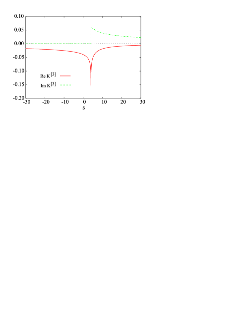
Figure 5: (Color online) $K^{[3]}(s;m_{1}^{2},m_{2}^{2})$ with $m_{1}\!=\!m_{2}\!=\!m\!=\!1$.

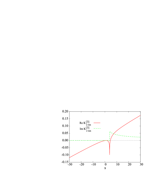
Figure 6: (Color online) $K^{[3]}_{2\,\mathrm{ren}}(s,m;m_{1}^{2},m_{2}^{2})$ with $m_{1}=m_{2}\!=\!m\!=\!1$.

We begin our iterations by calculating

$$G_{0}(s) \ =\ \frac{1}{m^{2}-s-i\epsilon}\>,$$ (176)

$$\Pi^{\mathrm{[sub\,1]}}_{0}(s) \ =\ \frac{1}{2}\ K^{[4]}_{1\,\mathrm{ren}}(s;m^{2},m^{2})\>,$$ (177)

$$D_{0}(s) \ =\ \frac{1}{-\,g_{R}^{-1}\ +\ \Pi^{\mathrm{[sub\,1]}}_{0}(s)}\>,$$ (178)

$$\Sigma^{\mathrm{[sub\,2]}}_{0}(s) \ =\ \int_{4m^{2}}^{\infty}\ \frac{\mathrm{d}(m_{1}^{2})}{\pi}\,\mathrm{Im}\,D_{0}(m_{1}^{2})\,K^{[4]}_{2\,\mathrm{ren}}(s;m_{1}^{2},m^{2})\>.$$ (179)

Subsequently we iterate

$$G_{1}(s)= \frac{1}{m^{2}-s+\Sigma^{\mathrm{[sub\,2]}}_{0}(s)}=G_{0}(s)-\Delta G(s)\>,$$ (180)

$$\Pi^{\mathrm{[sub\,1]}}_{1} (s)=\Pi^{\mathrm{[sub\,1]}}_{0}(s)$$ (181)

$$-\int_{9m^{2}}^{\infty}\ \frac{\mathrm{d}(m_{1}^{2})}{\pi}\ \mathrm{Im}\Delta G(m_{1}^{2})\ K^{[4]}_{1\,\mathrm{ren}}(s;m_{1}^{2},m^{2})$$

$$+\frac{1}{2}\int_{9m^{2}}^{\infty}\ \frac{\mathrm{d}(m_{1}^{2})}{\pi}\ \mathrm{Im}\Delta G(m_{1}^{2})$$

$$\qquad\times\int_{9m^{2}}^{\infty}\ \frac{\mathrm{d}(m_{2}^{2})}{\pi}\,\mathrm{Im}\Delta G(m_{2}^{2})K^{[4]}_{1\,\mathrm{ren}}(s;m_{1}^{2},m_{2}^{2})\>,$$

$$D_{1}(s)\ =\ \frac{1}{-\,g_{R}^{-1}\ +\ \Pi^{\mathrm{[sub\,1]}}_{1}(s)}\>,$$ (182)

$$\Sigma^{\mathrm{[sub\,2]}}_{1} (s)=\Sigma^{\mathrm{[sub\,2]}}_{0}(s)-\int_{4m^{2}}^{\infty}\frac{\mathrm{d}(m_{1}^{2})}{\pi}\,\mathrm{Im}D_{1}(m_{1}^{2})$$ (183)

$$\times\int_{9m^{2}}^{\infty}\ \frac{\mathrm{d}(m_{2}^{2})}{\pi}\ \mathrm{Im}\Delta G(m_{2}^{2})\ K^{[4]}_{2\,\mathrm{ren}}(s;m_{1}^{2},m_{2}^{2})\>.$$

The first iteration results are depicted in Fig. 3. Here, we compare our results with the leading order contribution in the perturbative reexpansion of $D(s)$ in powers of $\Pi(s)$, i.e.

$$D(s) \ =\ \frac{1}{-\,g_{R}^{-1}+\Pi(s)}$$ (184)

$$\ =\ -\ g_{R}\ -\ g_{R}^{2}\ [\Pi^{\mathrm{[sub\,1]}}(s)]^{2}\ -\ \cdots\>,$$

which is similar to the sunset approximation of Van Hees and Knoll.

The effect of the self-consistent calculation is depicted in Fig. 4. As stated by van Hees and Knoll ref:sunset , the first iteration results are negligibly modified by the subsequent iterations, since the main contributions come from the pole term of $G_{0}$, and the continuous corrections start at a threshold of $s=9m^{2}$. Henceforth, only the high momentum tail of the propagators is affected, and convergence is rapidly achieved.

IV.3 2+1 dimensions

The 2+1 dimensions case is different from the 3+1 dimensions case for two reasons. The first is that the vacuum polarization goes to zero at large momentum so that $D$ goes to a constant and obeys a once-subtracted dispersion relation. Secondly, the self-energy requires only one subtraction to make it finite. However, we will find it more convenient for our iterative scheme to use two subtractions so that the renormalized Green’s function has the same strength at the pole as the free one.

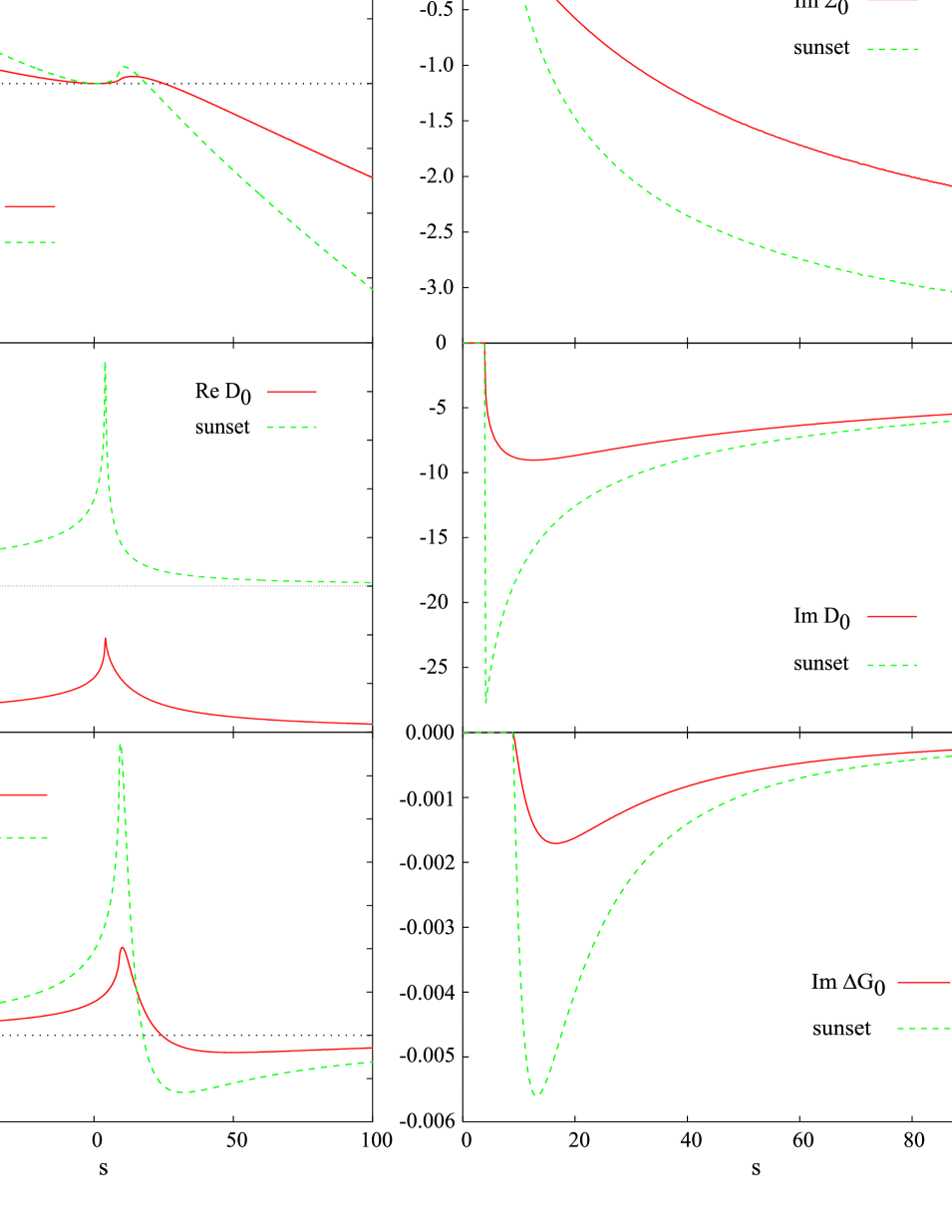
Figure 7: (Color online) First iteration results in 2+1 dimensions ($g$=30).

Using Eq. (151), the kernel $K^{[3]}(s;m_{1}^{2},m_{2}^{2})$ is evaluated for the domain $0<s\leq(m_{1}+m_{2})^{2}$, and the result is analytically continued outside this range. We obtain

$$K^{[3]}(s;m_{1}^{2},m_{2}^{2}) \ =\ \left\{\begin{array}[]{ll}-\ \frac{1}{4\pi\,\sqrt{|s|}}\ \tan^{-1}\frac{\sqrt{|s|}}{m_{1}+m_{2}}\>,&\mathrm{if}\ s\leq 0\>,\\ -\ \frac{1}{8\pi\,\sqrt{s}}\ \ln\frac{m_{1}+m_{2}+\sqrt{s}}{m_{1}+m_{2}-\sqrt{s}}\>,&\mathrm{if}\ 0\leq s<(m_{1}+m_{2})^{2}\>,\\ -\ \frac{1}{8\pi\,\sqrt{s}}\ \left[\ln\frac{\sqrt{s}+(m_{1}+m_{2})}{\sqrt{s}-(m_{1}+m_{2})}-i\,\pi\right]\>,&\mathrm{if}\ s\geq(m_{1}+m_{2})^{2}\>.\end{array}\right.$$ (188)

In Fig. 5 we depict the $s$-dependence of $K^{[3]}(s;m^{2},m^{2})$, which is related to the starting value of the polarization, $\Pi_{0}(s)$. We notice immediately that for large momentum, we have $K^{[3]}(s;m_{1}^{2},m_{2}^{2})\rightarrow 0$, like $1/{\sqrt{s}}$. In order to satisfy the boundary conditions required by the spectral representation, we use the simple manipulation

$$D(s) \ =\ -\ g\ +\ [D(s)+g]$$ (189)

$$\ =\ -\ g\ +\ \int_{4m^{2}}^{\infty}\ \frac{\mathrm{d}(m^{2})}{\pi}\ \frac{\mathrm{Im}\,D(m^{2})}{m^{2}-s-i\epsilon}\>,$$ (190)

which gives

$$\Sigma(s)=-ig\int[\mathrm{d}^{3}q]G(q^{2})+\int_{4m^{2}}^{\infty}\frac{\mathrm{d}(m_{1}^{2})}{\pi}\mathrm{Im}\,D(m_{1}^{2})$$

$$\qquad\times\int_{0}^{\infty}\frac{\mathrm{d}(m_{2}^{2})}{\pi}\mathrm{Im}G(m_{2}^{2})K^{[3]}(s;m_{1}^{2},m_{2}^{2})\>.$$ (191)

Thus we see that one subtraction (mass renormalization) is sufficient to render the theory finite. However making only one subtraction, i.e.

$$\Sigma^{\mathrm{[sub\,1]}}(m^{2}) \ =\ 0\>,$$ (192)

or

$$\Sigma^{\mathrm{[sub\,1]}}(s) \ \equiv\ \Sigma(s)\ -\ \Sigma(m^{2})\>,$$ (193)

one induces a finite wave function renormalization making the bare and renormalized Green’s functions having different strengths at the pole. To avoid this, it is convenient to do a complete physical renormalization even in 2+1 dimensions and instead consider:

$$\Sigma^{\mathrm{[sub\,2]}}(s)= \int_{4m^{2}}^{\infty}\frac{\mathrm{d}(m_{1}^{2})}{\pi}\mathrm{Im}\,D(m_{1}^{2})$$ (194)

$$\quad\times\int_{0}^{\infty}\frac{\mathrm{d}(m_{2}^{2})}{\pi}\mathrm{Im}G(m_{2}^{2})K^{[3]}_{2\,\mathrm{ren}}(s;m_{1}^{2},m_{2}^{2})\>,$$

where

$$K^{[3]}_{2\,\mathrm{ren}}(s;m_{1}^{2},m_{2}^{2})\,=\,K^{[3]}(s;m_{1}^{2},m_{2}^{2})-K^{[3]}(m^{2};m_{1}^{2},m_{2}^{2})$$

$$\qquad-(s-m^{2})\ \partial_{s}K^{[3]}(s;m_{1}^{2},m_{2}^{2})|_{s=m^{2}}\>.$$ (195)

For the range $0\leq s<(m_{1}+m_{2})^{2}$, we obtain

$$K^{[3]}_{2\,\mathrm{ren}} (s;m_{1}^{2},m_{2}^{2})\ =\ -\ \frac{1}{8\pi^{2}}\biggl{[}\frac{1}{\sqrt{s}}\ \ln\frac{m_{1}+m_{2}+\sqrt{s}}{m_{1}+m_{2}-\sqrt{s}}$$

$$\ -\ \Bigl{(}1-\frac{s-m^{2}}{2m^{2}}\Bigr{)}\ \ln\frac{m_{1}+m_{2}+m}{m_{1}+m_{2}-m}$$

$$\ -\ \frac{(s-m^{2})(m_{1}+m_{2})}{m^{2}\bigl{[}(m_{1}+m_{2})^{2}-m^{2}\bigr{]}}\biggr{]}\>.$$ (196)

The analytical continuation of the above result is done according to Eq. (188), and we illustrate in Fig. 6 the $s$-dependence of $K^{[3]}_{2\,\mathrm{ren}}(s;m^{2},m^{2})$.

For concreteness, we list the explicit equations we need the solve. For the first iteration, we have

$$G_{0}(s) =\frac{1}{m^{2}-s-i\epsilon}\>,$$ (197)

$$\Pi_{0}(s) =\frac{1}{2}\ K^{[3]}(s;m^{2},m^{2})\>,$$ (198)

$$D_{0}(s) =\frac{1}{-\,g^{-1}+\Pi_{0}(s)}\>,$$ (199)

$$\Sigma^{\mathrm{[sub\,2]}}_{0}(s) =\int_{4m^{2}}^{\infty}\frac{\mathrm{d}(m_{1}^{2})}{\pi}\ \mathrm{Im}D_{0}(m_{1}^{2})\,K^{[3]}_{2\,\mathrm{ren}}(s;m_{1}^{2},m^{2})\>,$$ (200)

while the subsequent iterations provide the solution of the system of equations

$$G_{1}(s)= \frac{1}{m^{2}-s+\Sigma^{\mathrm{[sub\,2]}}_{0}(s)}=G_{0}(s)-\Delta G(s)\>,$$ (201)

$$\Pi_{1} (s)=\Pi_{0}(s)$$ (202)

$$-\int_{9m^{2}}^{\infty}\ \frac{\mathrm{d}(m_{1}^{2})}{\pi}\ \mathrm{Im}\Delta G(m_{1}^{2})\ K^{[3]}(s;m_{1}^{2},m^{2})$$

$$+\frac{1}{2}\ \int_{9m^{2}}^{\infty}\ \frac{\mathrm{d}(m_{1}^{2})}{\pi}\ \mathrm{Im}\Delta G(m_{1}^{2})$$

$$\qquad\times\int_{9m^{2}}^{\infty}\ \frac{\mathrm{d}(m_{2}^{2})}{\pi}\ \mathrm{Im}\Delta G(m_{2}^{2})\ K^{[3]}(s;m_{1}^{2},m_{2}^{2})\>,$$

$$D_{1}(s)\ =\ \frac{1}{-\,g^{-1}\ +\ \Pi_{1}(s)}\>,$$ (203)

$$\Sigma^{\mathrm{[sub\,2]}}_{1} (s)=\Sigma^{\mathrm{[sub\,2]}}_{0}(s)-\int_{4m^{2}}^{\infty}\frac{\mathrm{d}(m_{1}^{2})}{\pi}\ \mathrm{Im}D_{1}(m_{1}^{2})$$ (204)

$$\times\int_{9m^{2}}^{\infty}\frac{\mathrm{d}(m_{2}^{2})}{\pi}\,\mathrm{Im}\Delta G(m_{2}^{2})K^{[3]}_{2\,\mathrm{ren}}(s;m_{1}^{2},m_{2}^{2})\>.$$

Similarly to the 3+1 dimensions case, we plot the results after the first iteration (see Fig. 7), and compare with the sunset-like approximation of van Hees and Knoll. Once again, we the corrections beyond the first iteration result are suppressed due to $(m_{1}+m_{2})^{2}$ threshold in the emergence of the kernels’ imaginary parts, and self-consistent result virtually lies on top of the first iteration result.

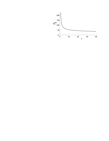
Figure 8: The cutoff, $\Lambda$, dependence of the maximum value of the renormalized coupling constant, $g_{R}^{\mathrm{max}}$.

V Effect of Landau Pole

What we have done earlier was a slight cheat for 3+1 dimensions in that $\lambda\phi^{4}$ field theory is only an effective field theory in 3+1 dimensions, having nontrivial scattering only when defined on the lattice (or with a momentum cutoff), and the lattice spacing not taken to zero phi4 . The range of validity of the effective theory is determined by the position of the Landau Pole. The bare coupling constant $\lambda$ must be positive for the lattice field theory to be defined. Using Eq. (85), we obtain the relationship

$$g_{R}\ =\ \frac{g}{1\ -\ g\,\Pi(0)}\>,$$ (205)

or

$$g\ =\ \frac{g_{R}}{1\ +\ g_{R}\,\Pi(0)}\>,$$ (206)

If we evaluate $\Pi(0)$ in leading order, integrating over $p_{0}$ and using a cutoff $\Lambda$ in $|{\vec{p}}|$ we have

$$\Pi(0)\ =\ -\ \frac{1}{16\pi^{2}}\int_{0}^{\Lambda}\frac{p^{2}\,\mathrm{d}p}{(p^{2}+m^{2})^{\frac{3}{2}}}\>.$$ (207)

The asymptotic behavior of the above expression at large cutoff, $\Lambda$, is

$$\Pi(0)\ =\ -\frac{1}{16\pi^{2}}\ \ln{\frac{2\Lambda}{m}}\>.$$ (208)

In the cutoff theory one has that $g_{R}$ is a monotonically increasing function of the bare coupling constant $g$, and has a maximum value defined by

$$g_{R}^{\mathrm{max}}\ =\ -\ \frac{1}{\Pi(0)}\ =\ 16\pi^{2}\ \Bigl{[}\ln\frac{2\Lambda}{m}\Bigr{]}^{-1}\>.$$ (209)

This behavior is shown in Fig. 8.

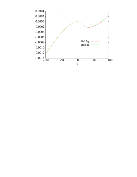
Figure 9: (Color online) Real part of the self-energy $\Sigma_{0}(s)$, in 3+1 dimensions, $g_{R}=1$.

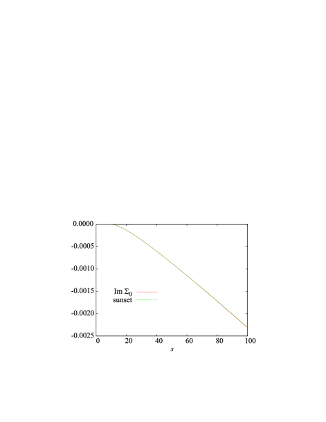
Figure 10: (Color online) Imaginary part of the self-energy $\Sigma_{0}(s)$, in 3+1 dimensions, $g_{R}=1$.

In order to capture all the physics of our approximation, we would like the cutoff, $\Lambda$, to be much larger than the $9m^{2}$ threshold, that is so important in getting the correct physics. Thus, any $\Lambda$ greater than say $30m^{2}$ will be sufficiently large. From Fig. 8, we conclude that as long as $g_{R}\sim 1$, there is a wide range of momenta for which the effective theory is valid, and we can expect there exists a regime of cutoffs (less than the maximum momentum) for which the theory becomes cutoff independent. This behavior was shown to be correct in our mean field simulations of disoriented chiral condensates dcc . In this regime, the continuum results we used here should offer a good approximation to the actual cutoff integrals required for consistency in order that $\phi^{4}$ field theory be a good effective field theory in the energy regime lower than the Landau cutoff for that coupling constant. To avoid Landau pole issues, using $g_{R}\leq 1$ is much more realistic than the value ($g_{R}$=30) chosen by van Hees and Knoll. In 3+1 dimensions at $g_{R}=1$, the resummed 1/N approximation and the sunset approximation are indeed very close. These results are illustrated in Figs. 9 and 10.

VI Conclusions

In this paper we have discussed the renormalization of the S-D equations of the auxiliary field formulation of $\phi^{4}$ field theory and then specialized to the self-consistent approximation to the coupled Green’s function equations obtained by ignoring vertex corrections or equivalently expanded the 2-PI generating functional in loops and keeping the two-loop contribution to $\Gamma_{2}$. We then obtained vacuum solutions for the self energy and vacuum polarization contribution to the inverse Green’s functions in the bare vertex approximation. We compared our results to the related sunset graph approximation of Van Hees and Knoll and discovered that at strong coupling there were significant differences in these two approximations. These differences become insignificant when $g_{R}$ is of order 1. In discussing the renormalization we confined ourselves to the case when there is no symmetry breakdown. When there is symmetry breakdown, one can use a “mass independent” renormalization scheme, such as that proposed by Kugo ref:Kugo , which requires only renormalizing the effective action in the symmetric theory, which is discussed here, to also renormalize the broken symmetry case. Otherwise, one can study the more complicated set of broken symmetry Dyson equations and renormalize those as discussed in Ref. Haymaker1 . The reason we chose physical on mass shell renormalization in this paper was that it allowed a clean iterative method for solving the self consistent S-D equations for the vacuum sector. For non-equilibrium uses of the effective action in the CTP formalism one does not need to rely on self consistent solutions, since the time update equations will find these solutions dynamically. In the latter case it might be more efficient to determine the renormalization counter terms using the mass independent strategy of Kugo.

An important question we have not addressed here is the fulfilment of Ward identities. In obtaining the renormalized S-D equations, we relied on the Ward identity $Z_{1}=Z_{2}$ to obtain our final result for the exact renormalized Green functions. After doing that we noticed it was consistent up to order $1/N$ to set the “renormalized” vertex function to 1. In leading order (and beyond) in traditional large-N expansions of the auxiliary field generating functional, one explicitly can verify (as well as prove order by order) that $Z_{1}=Z_{2}$, and also the Ward identities related to the O(N) symmetry, are satisfied order by order. However, the resummation inherent in the self consistently determined 2-PI effective action can violate the exact Ward identities since one now has a result exact to a particular order in $1/N$, but different quantities (for example $Z_{1}$ and $Z_{2}$) may differ in the coefficients of the $1/N^{2}$ and higher terms when the relevant Green functions are reexpanded in a series in $1/N$. Therefore, although we have obtained finite renormalized S-D equations, which are exact to order $1/N$ one cannot rule out order $(1/N^{2})$ violations of Ward identities, Goldstone theorems etc. To obtain approximations in the 2-PI formalism which are consistent with Ward identities and gauge invariance (for gauge theories) is still an unsolved problem and the subject of lots of recent attention ref:VanHees66 ; ward . This subject is beyond the scope of this paper, which is mainly concerned with obtaining finite renormalized S-D equations for the truncated hierarchy of Green functions. In a future publication, we will use the results presented here to study the thermalization of renormalized $\phi^{4}$ field theory in 2+1 and 3+1 dimensions for both $N=1$ and the $N=4$ O(N) model and study the grid sizes needed for the renormalized theory to be independent of grid size.

- (1) J. M. Luttinger and J. C. Ward, Phys. Rev. 118, 1417 (1960); G. Baym, Phys. Rev. 127, 1391 (1962); H. D. Dahmen and G. Jona Lasino, Nuovo Cimento, 52A, 807 (1962); J. M. Cornwall, R. Jackiw and E. Tomboulis, Phys. Rev. D 10, 2428 (1974).
- (2) J. P. Blaizot, E. Iancu and A. Rebhan Phys. Rev. Lett. 83, 2906 (1999) [hep-ph/9906340]; U. Kraemmer and A. Rebhan, Rep. Prog. Phys. 67, 351 (2004) [hep-ph/0310337].
- (3) H. van Hees and J. Knoll, Phys. Rev. D 65, 025010 (2002) [hep-ph/0107200].
- (4) H. Van Hees and J. Knoll, Phys. Rev. D 65, 105005 (2002) [hep-ph/0111193].
- (5) E. Calzetta and B. L. Hu, Phys. Rev. D 35, 495 (1987).
- (6) B. Mihaila, F. Cooper and J. F.Dawson, Phys. Rev. D 63, 096003 (2001) [hep-ph-0006254]; K. Blagoev, F. Cooper, J. F. Dawson and B. Mihaila, Phys.Rev. D. 64, 125003 (2001) [hep-ph/0106195]; F. Cooper, J. F. Dawson and B. Mihaila, Phys. Rev. D 67, 051901R (2003) [hep-ph/0207346 ]; F. Cooper, J. F. Dawson, and B. Mihaila, Phys. Rev. D 67, 056003 (2003) [hep-ph/0209051]; B. Mihaila, Bogdan Mihaila, Phys. Rev. D 68, 36002 (2003) [hep-ph/0303157].
- (7) J. Berges and J. Cox, Phys. Lett B517, 369 (2001) [hep-ph/0006160]; G. Aarts and J. Berges, Phys. Rev. D, 64, 105010 (2001) [hep-ph/0103049]; J. Berges, Nucl. Phys. A699, 847 (2002) [hep-ph/0105311]; G. Aarts and J. Berges, Phys. Rev. Lett. 88, 041603 (2002) [hep-ph/0107129]; J. Berges and J. Serreau, [hep-ph/0302210]
- (8) G. Aarts, D. Ahrensmeier, R. Baier, J. Berges, and J. Serreau, Phys. Rev. D 66, 045008 (2002) [hep-ph/0201308].
- (9) J. Berges and J. Serreau, Phys. Rev. Lett. 91, 111601 (2003) [hep-ph/0208070].
- (10) J. Berges, S. Borsanyi, and J. Serreau, Nucl. Phys. B660, 51 (2003) [hep-ph/0212404].
- (11) M. Alford, J. Berges, J. M. Cheyne [hep-ph/0404059].
- (12) J. Baacke and A. Heinen, Phys. Rev. D 67, 105020 (2003) [hep-ph/0212312]; J. Baacke and A. Heinen, Phys. Rev. D 68, 127702 (2003) [hep-ph/0305220]; J. Baacke and A. Heinen, Phys. Rev. D 69, 083523 (2004) [hep-ph/0311282].
- (13) S. Juchem, W. Cassing, C. Greiner, Phys. Rev. D 69, 025006 (2004) [hep-ph/0307353].
- (14) G. Aarts and J. M. M. Resco, Phys. Rev. D 68, 085009 (2003) [hep-ph/0303216]; G. Aarts and J. M. M. Resco, J. High Energy Phys. 0402, 061 (2004) [hep-ph/0402192].
- (15) F. Cooper, B. Mihaila and J. F. Dawson, Phys. Rev. D 56, 5400 (1997) [hep-ph/9705354]; L. M. Bettencourt and C. Wetterich, Phys. Lett. B430, 140 (1998) [hep-ph/9712429]; B. Mihaila, T. Athan, F. Cooper, J. Dawson and S. Habib, Phys. Rev. D 62, 125015 (2000) [hep-ph/0003105].
- (16) E. Calzetta and B. L. Hu, Phys. Rev. D 37, 2878 (1988).
- (17) J.-P. Blazot, E. Iancu and U. Reinosa, Phys. Lett. B568, 160 (2003) [hep-ph/0301201].
- (18) N. N. Bogoliubov and O. S. Parasiuk, Acta Math. 97, 227 (1957); K. Hepp, Comm. Math. Phys. 2, 301 (1966); W. Zimmermann, Commun. Math. Phys. 15, 208 (1969).
- (19) G. ’t Hooft and M .J. G. Veltman, Nucl. Phys. B44, 189 (1972).
- (20) J. D. Bjorken and S. D. Drell, Relativistic Quantum Fields, McGraw-Hill (1965), p 334.
- (21) F. Cooper, G. Guralnik, R. Haymaker and K. Tamvakis, Phys. Rev 20, 3336 (1979); R. Haymaker and F. Cooper, Phys. Rev. 19, 562 (1979).
- (22) J. Schwinger, J. Math. Phys. 2, 407 (1961); L. V. Keldysh Zh. Eksp. Teor. Fiz. 47, 1515 (1964) [Sov. Phys. JETP 20, 1018 (1965)]; G. Zhou, Z. Su, B. Hao, and L. Yu, Phys. Rep. 118, 1 (1985).
- (23) F. Cooper, Y. Kluger, E. Mottola, and J. P. Paz, Phys. Rev. D 51, 2377 (1995) [hep-ph/9404357]; M. A. Lampert, J. F. Dawson, and F. Cooper, Phys. Rev. D 54, 2213 (1996) [hep-th/9603068].
- (24) F. Cooper, S. Habib, Y. Kluger, E. Mottola, J. P. Paz, and P. Anderson, Phys. Rev. 50, 2848 (1994).
- (25) L.M. Bettencourt, F. Cooper and K. Pao, Phys. Rev. Lett. 89, 112301 (2002) [hep-ph/0109108].
- (26) K. Wilson, Phys. Rev. D 7, 2911 (1973); J. Cornwall, R. Jackiw, and E. Tomboulis, Phys. Rev. D 10, 2424 (1974); S. Coleman, R. Jackiw and H. D. Politzer, Phys. Rev. D 10, 2491 (1974).
- (27) R. Root, Phys. Rev. D 11, 831 (1975).
- (28) C. M. Bender, F. Cooper, and G. S. Guralnik, Ann. Phys. (N.Y.) 109, 165 (1977).
- (29) J. Kogut and K. Wilson, Phys. Rep. 12C, 75 (1974); G. A. Baker and J. M. Kincaid, Phys. Rev. Lett. 42, 1431(1979); C. M. Bender, F. Cooper and G. S. Guralnik, Phys. Rev. Lett. 45, 501 (1980); G. A. Baker Jr., L. P. Benofy, F. Cooper, and D. Preston, Nucl. Phys. B210, 273 (1982); D. J. E. Callaway, Phys. Rep. 167, 241 (1988).
- (30) B. W. Lee, Nucl. Phys. B9, 649 (1969); J. L. Gervais and B. W. Lee, Nucl. Phys. B12, 627 (1969); S. Weinberg, Phys. Rev. D 8, 3497 (1973); G. ’t Hooft, Nucl. Phys. B61, 455, (1973).
- (31) D. J. Gross, “Applications of the Renormalization Group to High Energy,” in Methods in Field Theory, Les Houches 1975, Amsterdam, pp. 141-250 (1976).
- (32) W. H. L. Furry, Phys. Rev. 51, 125 (1937).
- (33) Claude Itzykson and Jean-Bernard Zuber, Quantum Field Theory, McGraw-Hill (1980), p 376.
- (34) T. Kugo, Prog. Theor. Phys. 57 593 (1957)
- (35) H. van Hees and J. Knoll, Phys. Rev. D 66, 025028 (2002) [hep-ph/0203008].
- (36) H. Van Hees and J. Knoll, [hep-ph/0210262]; E. Mottola, “Gauge invariance in 2PI effective actions,” in Strong and Electroweak Matter 2002: Proceedings of the SEWM 2002 Meeting, World Scientific, N.Y., pp. 432-436 (2002)