Statistical hadronization and hadronic microcanonical ensemble II

Abstract

We present a Monte-Carlo calculation of the microcanonical ensemble of the of the ideal hadron-resonance gas including all known states up to a mass of about 1.8 GeV and full quantum statistics. The microcanonical average multiplicities of the various hadron species are found to converge to the canonical ones for moderately low values of the total energy, around 8 GeV, thus bearing out previous analyses of hadronic multiplicities in the canonical ensemble. The main numerical computing method is an importance sampling Monte-Carlo algorithm using the product of Poisson distributions to generate multi-hadronic channels. It is shown that the use of this multi-Poisson distribution allows an efficient and fast computation of averages, which can be further improved in the limit of very large clusters. We have also studied the fitness of a previously proposed computing method, based on the Metropolis Monte-Carlo algorithm, for event generation in the statistical hadronization model. We find that the use of the multi-Poisson distribution as proposal matrix dramatically improves the computation performance. However, due to the correlation of subsequent samples, this method proves to be generally less robust and effective than the importance sampling method.

1 Introduction

The basic assumption of the statistical hadronization model (SHM) is that, as a consequence of a dynamical QCD-driven process, the final stage of a high energy collision gives rise to the formation a set of colourless massive extended objects, defined as clusters (or fireballs). They are assumed to produce hadrons in a purely statistical manner, namely all multihadronic states within the cluster volume and compatible with its quantum numbers are equally likely. The set of equiprobable states with fixed four-momentum and internal charges (abelian or not) is what is usually called the microcanonical ensemble . Interactions between stable hadrons are mostly taken into account by the inclusion of all resonances as independent states bdm , which is the reason of the usual expression, in the SHM, of ideal hadron-resonance gas hage .

The special motivations for a detailed study of the microcanonical ensemble of the ideal hadron-resonance gas have been extensively discussed in the first paper beca1 . They can be shortly summarized as:

1. The need of a tool to hadronize final-state clusters in particle and heavy ion collisions in the statistical hadronization model and test observables which cannot be calculated analytically.

2. The assessment of the validity of previous calculations in the canonical ensemble, especially in the analysis of average multiplicities in high energy elementary collisions beca ; becaheinz ; becagp .

The first point is quite clear: if we could compute microcanonical averages numerically in a practical way, we would be able to make predictions on many observables within the basic framework of the statistical model without invoking further assumptions or approximations which are needed to obtain analytical expressions. Furtermore, the availability of a Monte-Carlo integration algorithm opens the way to event generators with hadronization stage modelled by SHM. The second point is somehow related to the first. Indeed, in previous work within SHM, specific assumptions were invoked in order to allow the use of the canonical ensemble, which is far easier to handle with regard to both analytical and numerical calculations. It is then necessary to verify whether it was sound to calculate multiplicities in the canonical ensemble by comparing them to those in the microcanonical ensemble with the same values of total mass and volume.

The microcanonical formalism for the hadron gas and the relation between microcanonical and canonical ensembles have been developed in the first paper beca1 . In this paper we will focus on the numerical analysis; we will discuss the main computational issues and we will describe two algorithms to sample the microcanonical hadron gas phase space. As has been mentioned above, we will inspect the differences between microcanonical and canonical averages. In this first study, we will only deal with observables pertaining to particle multiplicities, leaving the analysis of momentum spectra to further works.

The microcanonical ensemble of the hadron gas has been investigated numerically by K. Werner and J. Aichelin weai by using a Monte-Carlo method based on Metropolis algorithm. Results on specific observables have recently been published liu in a hadron gas model including fundamental multiplets (two meson nonets and baryon octet plus decaplet). In comparison with these previous works, we will show calculations for the full hadron gas including all known species (more than 250) up to a mass of about 1.8 GeV and, particularly, we will introduce a new updating rule for Metropolis algorithm leading to a dramatic improvement of its performance in terms of computing time. Moreover, we propose a different Monte-Carlo computing method, based on the importance sampling of multi-hadronic channel space, which proves to be more effective than Metropolis algorithm for the calculation of averages.

The paper is organized as follows: the basic microcanonical formalism is summarized in Sect. 2; the numerical method to compute the phase space volumes for a given multi-hadronic channel is discussed in Sect. 3; in Sect. 4 we describe the importance sampling method which is well suited to compute averages in the microcanonical ensemble of the ideal hadron-resonance gas; in Sect. 5 we show the comparison between microcanonical and canonical averages; in Sect. 6 and 7 the Metropolis algorithm is studied in detail; finally, conclusions are summarized in Sect. 8.

2 Microcanonical partition function

In principle, any average on a given statistical mechanics ensemble could be calculated from the partition function. The microcanonical partition function of the hadron gas is best defined beca1 as the sum over all multihadronic states localized within the cluster $|h_{V}\rangle$ constrained with four-momentum and abelian (i.e. additive) charge conservation:

$$\Omega=\sum_{h_{V}}\langle h_{V}|\delta^{4}(P-P_{\rm op})\delta_{{\bf Q},{\bf Q}_{\rm op}}|h_{V}\rangle$$ (1)

where ${\bf Q}=(Q_{1},\ldots,Q_{M})$ is a vector of $M$ integer abelian charges (electric, baryon number, strangeness etc.), $P$ the four-momentum of the cluster and $P_{\rm op}$, ${\bf Q}_{\rm op}$ the relevant operators. Provided that relativistic quantum field effects are neglected and the volume of the cluster is large enough to allow the approximation of finite-volume Fourier integrals with Dirac deltas, it can be proved beca1 that $\Omega$ can be written as a multiple integral:

$$\Omega=\frac{1}{(2\pi)^{4+M}}\int{\rm d}^{4}y\;{\rm e}^{{\rm i}P\cdot y}\int_{-\mbox{\boldmath${\scriptstyle{\pi}}$}}^{+\mbox{\boldmath${\scriptstyle{\pi}}$}}{\rm d}^{M}\phi\;{\rm e}^{{\rm i}{\bf Q}\cdot\mbox{\boldmath${\scriptstyle{\phi}}$}}$$

$$\times\exp\Big{[}\sum_{j}\frac{(2J_{j}+1)V}{(2\pi)^{3}}\!\!\!\int{\rm d}^{3}{\rm p}\;\log(1\pm{\rm e}^{-{\rm i}p_{j}\cdot y-{\rm i}{\bf q}_{j}\cdot\mbox{\boldmath${\scriptstyle{\phi}}$}})^{\pm 1}\Big{]}$$ (2)

where ${\bf q}_{j}$ is the vector of the abelian charges for the $j^{\rm th}$ hadron species, $J_{j}$ its spin, $V$ the volume of the cluster; the upper sign applies to fermions, the lower to bosons. The integral (2) is more easily calculable in the rest frame of the cluster where $P=(M,{\bf 0})$. Unfortunately, an analytical solution with no charge constraint (the so-called grand-microcanonical partition function) is known only in two limiting cases: non-relativistic and ultra-relativistic (i.e. with all particle masses set to zero). The full relativistic case has been attacked with several kinds of expansions cerhag1 but none of them proved to be fully satisfactory as the achieved accuracy in the estimation of different kinds of averages could vary from some percent to a factor 10. Therefore, a numerical integration of Eq. (2) is needed. The most suitable method is to decompose $\Omega$ into the sum of the phase space volumes with fixed particle multiplicities for each species:

$$\Omega=\sum_{{\{N_{j}\}}}\Omega_{{\{N_{j}\}}}{\delta_{{\bf Q},\sum_{j}N_{j}{\bf q}_{j}}}$$ (3)

${\{N_{j}\}}$ being a vector of $K$ integer numbers $(N_{1},\ldots,N_{K})$, i.e. the multiplicities of all of the $K$ hadronic species. The set of integers ${\{N_{j}\}}$ is also defined as a channel because it characterizes a specific decay channel of the cluster. The general phase space volume $\Omega_{\{N_{j}\}}$ for the channel ${\{N_{j}\}}$ obtained from can be written as a cluster decomposition. Let $j$ be the integer index running over all hadron species, and $\{h_{n_{j}}\}$ a partition (relevant to the species $j$) of $N_{j}$ in the multiplicity representation, i.e. a set of integers such that $N_{j}=\sum_{n_{j}=1}^{N_{j}}n_{j}h_{n_{j}}$; let $H_{j}=\sum_{n_{j}=1}^{N_{j}}h_{n_{j}}$ and let $c_{l_{j}}$ be the cyclic permutations of the first $n_{l_{j}}$ integers determined by the partition, with $\sum_{l_{j}=1}^{H_{j}}n_{l_{j}}=N_{j}$. Provided that relativistic quantum field effects are neglected (which is possible if the cluster linear size is greater than pion Compton wavelength, 1.4 fm), the phase space volume for fixed multiplicities reads beca1 :

$$\!\!\!\!\!\!\!\!\Omega_{{\{N_{j}\}}} = \int{\rm d}^{3}{\rm p}_{1}\ldots{\rm d}^{3}{\rm p}_{N}\;\delta^{4}(P-P_{f})$$ (4)

$$\times \prod_{j}\sum_{\{h_{n_{j}}\}}\frac{(\mp 1)^{N_{j}+H_{j}}(2J_{j}+1)^{H_{j}}}{\prod_{n_{j}=1}^{N_{j}}n_{j}^{h_{n_{j}}}h_{n_{j}}!}\prod_{l_{j}=1}^{H_{j}}F_{n_{l_{j}}}$$

where $P_{f}$ is the sum of all particle four-momenta. The factors $F_{n_{l_{j}}}$ in the equation above are Fourier integrals over the cluster region with proper volume $V$:

$$F_{n_{l_{j}}}=\prod_{i_{l_{j}}=1}^{n_{l_{j}}}\frac{1}{(2\pi)^{3}}\int_{V}{\rm d}^{3}{\rm x}\;{\rm e}^{{\rm i}{\bf x\cdot}({\bf p}_{i_{l_{j}}}-{\bf p}_{c_{l_{j}}(i_{l_{j}})})}$$ (5)

and the ${\bf p}$’s are the particle momenta. For sufficiently large $V$, the integral in Eq. (5) tends to a product of Dirac delta distribution and, if we use this limit in Eq. (4), we arrive at this expression of $\Omega_{\{N_{j}\}}$:

$$\!\!\!\!\!\!\!\!\Omega_{{\{N_{j}\}}} = \Bigg{[}\prod_{j}\sum_{\{h_{n_{j}}\}}(\mp 1)^{N_{j}+H_{j}}\frac{1}{\prod_{n_{j}=1}^{N_{j}}n_{j}^{4h_{n_{j}}}h_{n_{j}}!}$$ (6)

$$\Big{[}\prod_{l_{j}=1}^{H_{j}}\frac{V(2J_{j}+1)}{(2\pi)^{3}}\int{\rm d}^{3}{\rm p}^{\prime}_{l_{j}}\Big{]}\Bigg{]}\delta^{4}(P-\!\!\!\sum_{j,l_{j}=1}^{H_{j}}\!\!p^{\prime}_{l_{j}})$$

where, for a set of partitions ${\{h_{n_{1}}\}},\ldots,{\{h_{n_{K}}\}}$ for each of the hadron species, the four-momenta $p^{\prime}_{l_{j}}$ are those of lumps of particles of the same species $j$ ($H_{j}$ in number) with mass $n_{j}m_{j}$ and spin $J_{j}$.

For sufficiently large volumes, the leading term in Eq. (6), henceforth defined as $\Omega_{\{N_{j}\}}^{c}$, is that with the maximal power of $V$, i.e. with $H_{j}=N_{j}\;\forall j$. This term corresponds to the partitions ${\{h_{n_{j}}\}}=(N_{j},0,\ldots)\;\forall j$, namely to one particle per lump, and reads:

$$\Omega_{\{N_{j}\}}^{c}=$$

$$=\prod_{j}\frac{V^{N_{j}}(2J_{j}+1)^{N_{j}}}{(2\pi)^{3N_{j}}N_{j}!}\int{\rm d}^{3}{\rm p}_{1}\ldots{\rm d}^{3}{\rm p}_{N}\;\delta^{4}(P-\sum_{i=1}^{N}p_{i})$$ (7)

where $N=\sum_{j}N_{j}$. This is indeed the phase space volume in the classical Boltzmann statistics. Therefore, the terms beyond the leading one (2) in the expansions (4) and (6) account for the quantum statistics effects. The very same expression (2) holds as the leading term of the more general cluster decomposition (4). In fact, the cyclic permutations $c_{l_{j}}$ corresponding to the partition ${\{h_{n_{j}}\}}=(N_{j},0,\ldots)$ are identities, thus implying, according to Eq. (5):

$$\prod_{l_{j}=1}^{N_{j}}F_{n_{l_{j}}}=\frac{V^{N_{j}}}{(2\pi)^{3N_{j}}}$$ (8)

In the present work, we have used the approximated expression (6) of Eq. (4) to evaluate the phase space volume for fixed multiplicities. For the considered cluster masses and volumes (see later on) this approximation is satisfactory for most observables, taking into account that the leading term (2) of the cluster decomposition is the same in both Eq. (4) and (6) and that subleading terms give at most a 10% correction to the leading term.

A nice feature of the cluster decomposition (6) is that every term of the expansion is an integral just like the classical phase space volume (2) with lumps replacing particles. Specifically, the Eq. (6) can be rewritten as:

$$\Omega_{{\{N_{j}\}}}=\sum_{\{h_{n_{1}}\},\ldots,\{h_{n_{K}}\}}\Bigg{[}\prod_{j}\frac{(\mp 1)^{N_{j}+H_{j}}}{\prod_{n_{j}=1}^{N_{j}}n_{j}^{4h_{n_{j}}}}\Bigg{]}\Omega_{{\{H_{j}\}}}^{c}$$ (9)

Note that the factor $\prod_{n_{j}=1}^{N_{j}}h_{n_{j}}!$ has been absorbed in $\Omega_{{\{H_{j}\}}}^{c}$ as it takes into account the identity of the lumps. This form of the cluster decomposition shows that in actual numerical calculations all of the terms can be computed with the same routine.

As has been mentioned in the introduction, in this paper we are mainly interested in the calculation of quantities relevant to particle multiplicities and not to their momenta, namely their kinematical state. The average of an observable $O$ depending on particle multiplicities in the microcanonical ensemble can then be written as:

$$\langle O\rangle=\frac{\sum_{{\{N_{j}\}}}O({\{N_{j}\}})\Omega_{\{N_{j}\}}{\delta_{{\bf Q},\sum_{j}N_{j}{\bf q}_{j}}}}{\sum_{{\{N_{j}\}}}\Omega_{\{N_{j}\}}{\delta_{{\bf Q},\sum_{j}N_{j}{\bf q}_{j}}}}$$ (10)

Altogether, what we need to calculate in order to evaluate an average (10) are integrals like (6) and (2). The description of a suitable numerical technique to do that is the subject of next section.

3 Numerical calculation of the phase space volume

In order to calculate efficiently and quickly the phase space volume for fixed multiplicities $\Omega_{\{N_{j}\}}$ in Eq. (6), we have adopted a Monte-Carlo integration method proposed by Cerulus and Hagedorn in the 60’s cerhag1 ; cerhag2 and later employed by Werner and Aichelin weai . The method is described in detail in ref. weai . As we made only slight modifications, we just sketch it here; a more detailed description is given in Appendix A. As has already been mentioned, every term in the cluster decomposition (6) is an integral of the kind (2) and can be calculated by the same numerical method.

The calculation is carried out in the cluster’s rest frame, where $P=(M,{\bf 0})$ and $V$ is the proper volume. The integral (2) is first written as the product:

$$\Omega_{\{N_{j}\}}^{c}=\frac{V^{N}T^{3N-4}}{(2\pi)^{3N}}\prod_{j}\frac{(2J_{j}+1)^{N_{j}}}{N_{j}!}\;\Phi(M,m_{1},\ldots,m_{N})$$ (11)

where $T=M-\sum_{i=1}^{N}m_{i}$ is the available total kinetic energy for the $N$ particles (or lumps), and $\Phi$ is an adimensional kinematic integral:

$$\Phi=\frac{1}{T^{3N-4}}\int{\rm d}^{3}{\rm p}_{1}\ldots{\rm d}^{3}{\rm p}_{N}\;\delta^{4}(P-\sum_{i=1}^{N}p_{i})$$ (12)

After a sequence of variable changes, the function $\Phi$ is rewritten as an integral of an adimensional function $\Upsilon$ of $N-1$ variables $r_{i}\in[0,1]$ (see Appendix A):

$$\Phi=\int_{0}^{1}{\rm d}r_{1}\ldots\int_{0}^{1}{\rm d}r_{N-1}\;\Upsilon(r_{1},\ldots,r_{N-1})$$ (13)

which can be estimated through Monte-Carlo integration as:

$$\Phi\doteq\frac{1}{N_{S}}\sum_{k=1}^{N_{S}}\Upsilon(r_{1}^{(k)},\ldots,r_{N-1}^{(k)})$$ (14)

where $r_{i}^{(k)}$ are random numbers uniformely distributed in the interval $[0,1]$ and $N_{S}$ is the number of samples.

In order to calculate the full cluster decomposition of the phase space volume, in Eq. (9), the above calculation is repeated for all of the terms. To reduce the number of calls to the random number generation subroutine, one can take advantage of rewriting Eq. (9) as:

$$\Omega_{{\{N_{j}\}}}= \sum_{\{h_{n_{1}}\},\ldots,\{h_{n_{K}}\}}\Bigg{[}\prod_{j}\frac{(\mp 1)^{N_{j}+H_{j}}(2J_{j}+1)^{H_{j}}}{\prod_{n_{j}=1}^{N_{j}}n_{j}^{4h_{n_{j}}}h_{n_{j}}!}\Bigg{]}$$ (15)

$$\times\frac{V^{H}T^{3H-4}}{(2\pi)^{3H}}\Phi(M,\mu_{1},\ldots,\mu_{H})$$

where $\mu_{i}$ are meant to be the masses of the lumps defined by the partitions $\{h_{n_{j}}\}$ and $H=\sum_{j}H_{j}$. Since $H\leq N$, the first $H-1$ random numbers, out of $N-1$ extracted, can be used to estimate the $\Phi$ integral, according to Eq. (14), for each term in Eq. (15).

Figure 1: Distribution of $\Omega_{\{N_{j}\}}$ values computed with a numerical Monte-Carlo integration based on 1000 random samples, along with gaussian fits, for a cluster of 4 GeV mass and 0.4 GeV/fm³ energy density. Three channels are shown: (a) $\pi^{0},\pi^{0},\pi^{+},\pi^{-}$; (b) $\pi^{0},\pi^{0},\pi^{+},\pi^{+},\pi^{-},\pi^{-}$; (c) $\eta,\eta,\eta,\eta$. Top plots refer to the full quantum statistics calculation while those below to the classical statistics approximation.

For $N_{S}=1000$ random samples, the accuracy of the Monte-Carlo integration is satisfactory for all channels and turns out to be of the order of some percent. This may not be sufficient if one is interested in accurate calculations of single channel rates themselves, but is very good for the estimate of other, more inclusive, averages such as mean multiplicities, multiplicity distributions etc., in which the errors on different channels add incoherently (see Eq. (10)) and the relative statistical error is therefore greatly reduced with respect to that on the single term $\Omega_{{\{N_{j}\}}}$. In fig. 1 we show the gaussian distributions obtained by repeating 10000 times the calculation of $\Omega_{\{N_{j}\}}$ for three different channels in a cluster with 4 GeV mass and 0.4 GeV/fm³ energy density. The plots on the top row refer to the $\Omega_{\{N_{j}\}}$ value calculated in full quantum statistics, according to Eq. (6), and those on the bottom row in classical statistics, i.e. retaining only the leading term (2). It can be seen that the central values in full quantum statistics are higher than their classical approximations, as expected for channels involving identical bosons. The calculation in full quantum statistics with the exact expression (4) for finite volume yields results very close to those obtained with the approximated one (6). The spread in value of the statistical error (see resolutions quoted in fig. 1) is owing to the different multiplicities and masses of the particles in the channels. However, this spread is fairly small and stays well below an order of magnitude so that, in fact, a fixed number of Monte-Carlo samples $N_{S}$ is appropriate to calculate most $\Omega_{\{N_{j}\}}$’s with a given accuracy independently of particle content.

Figure 2: CPU time needed to calculate the phase space volume of a channel with $N$ neutral pions in a cluster with mass $N(m_{\pi^{0}}+500\;{\rm MeV})$ and energy density 0.4 GeV/fm³. The full dots refer to classical statistics and the hollow dots to full quantum statistics; lines are drawn to guide the eye. The CPU time has been normalized to a Pentium IV processor with 2 GHz clock rate.

The actual CPU time needed for the calculation of $\Omega_{\{N_{j}\}}$ with 1000 random samples is reasonably small. This is shown in fig. 2 for channels with $N$ neutral pions in a cluster with mass $N(m_{\pi^{0}}+500\;{\rm MeV})$ and energy density 0.4 GeV/fm³. In a full quantum statistics calculation, including lumps up to 5 particles, the CPU time is much larger because of the extra terms in the cluster decomposition. The time needed to calculate the integral (2) increases almost exponentially with the number of particles $N$ at low $N$, whereas at $N=11$ it features a drop due to a switch in the numerical method (see Appendix A) and flattens out thereafter. In quantum statistics, even at high $N$, there are many phase space integrals in the cluster decomposition to be calculated with the same method as for the classical terms at low $N$, thus the CPU time steadily increases, though not as steeply as for the classical term alone.

4 Importance sampling of microcanonical ensemble

As has been discussed previously, our goal is to develop a fast and accurate numerical method to calculate averages like (10) in the microcanonical ensemble. Being able to effectively calculate $\Omega_{\{N_{j}\}}$ for any channel, a brute force option is to do it for all of them. However, this method is not appropriate for a system like the hadron gas, because the actual number of channels is huge. Indeed, with 271 light-flavoured hadrons and resonances (those included in the latest Particle Data Book issue pdg ), the number of channels allowed by energy-momentum conservation is enormous and it increases almost exponentially with cluster mass (see fig. 3), involving an unacceptably large computing time. For instance, the CPU time needed to compute $\Omega_{\{N_{j}\}}$ for all of the 23 millions of channels of a cluster with 4 GeV mass is around 400 hours. Charge constraints can indeed reduce significantly the number of allowed channels, yet not enough. Therefore, the calculation of the phase space volume of all allowed channels is possible only for very light clusters, in practice lighter than $\approx 2$ GeV.

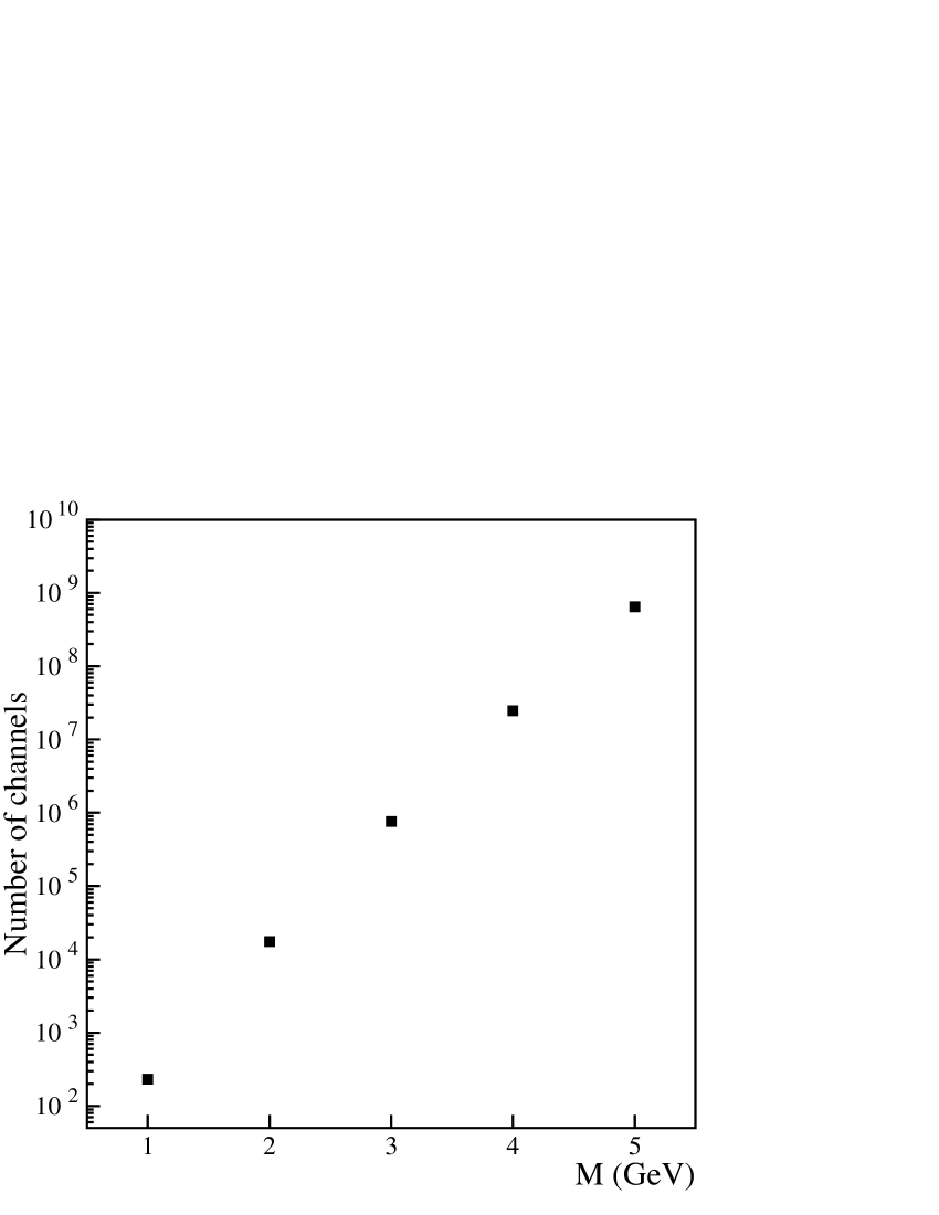
Figure 3: Number of allowed channels as a function of cluster mass in a hadron gas with 271 species and free charges.

Hence, if a method based on the exhaustive exploration of the channel space is not affordable, one has to resort to Monte-Carlo methods, whereby the channel space is randomly sampled.

An estimate of the average (10) can be made by means of the so-called importance sampling method. The idea of this method is to sample the channel space (i.e. the set of integers $N_{j}$, one for each hadron species) not uniformely, rather according to an auxiliary distribution $\Pi_{\{N_{j}\}}$ which must be suitable to being sampled very efficiently to keep computing time low, and, at the same time, as similar as possible to the distribution $\Omega_{\{N_{j}\}}$. The latter requirement is dictated by the fact that $\Omega_{\{N_{j}\}}$ is sizeable over a very small portion of the whole channel space. Hence, if random configurations were generated uniformely, for almost all of them $\Omega_{\{N_{j}\}}$ would have a negligible value, thus a huge number of samples would be required to achieve a good accuracy. On the other hand, if samples are drawn according to a distribution similar to $\Omega_{\{N_{j}\}}$, little time is wasted to explore unimportant regions and the estimation of the average (10) is more accurate. A crucial requirement for $\Pi_{\{N_{j}\}}$ is not to be vanishing or far smaller than $\Omega_{\{N_{j}\}}$ anywhere in its domain in order not to exclude some good regions from being sampled, thereby biasing the calculated averages in a finite statistics calculation.

Rewriting Eq. (10) as:

$$\langle O\rangle=\frac{\sum_{{\{N_{j}\}}}O({\{N_{j}\}}){\displaystyle\frac{\Omega_{\{N_{j}\}}}{\Pi_{\{N_{j}\}}}}\Pi_{\{N_{j}\}}{\delta_{{\bf Q},\sum_{j}N_{j}{\bf q}_{j}}}}{\sum_{{\{N_{j}\}}}{\displaystyle\frac{\Omega_{\{N_{j}\}}}{\Pi_{\{N_{j}\}}}}\Pi_{\{N_{j}\}}{\delta_{{\bf Q},\sum_{j}N_{j}{\bf q}_{j}}}}$$ (16)

makes it apparent that a Monte-Carlo estimate of $\langle O\rangle$ is:

$$\langle O\rangle\doteq\frac{\sum_{k=1}^{M}O({\{N_{j}\}}^{(k)}){\displaystyle\frac{\Omega_{\{N_{j}\}}^{(k)}}{\Pi_{\{N_{j}\}}^{(k)}}}}{\sum_{k=1}^{M}{\displaystyle\frac{\Omega_{\{N_{j}\}}^{(k)}}{\Pi_{\{N_{j}\}}^{(k)}}}}$$ (17)

where ${\{N_{j}\}}^{(k)}$ are samples of the channel space extracted according to the distribution $\Pi$ and fulfilling the charge constraint ${\bf Q}=\sum_{j}N_{j}{\bf q}_{j}$.

Provided that $M$ is large enough so that the distributions of both numerator and denominator in Eq. (17) are gaussians (hence the conditions of validity of the central limit thoerem are met), the statistical error $\sigma_{\langle O\rangle}$ on the average ${\langle O\rangle}$ can be estimated as (see Appendix B):

$$\sigma_{{\langle O\rangle}}^{2} = \frac{1}{M\Omega^{2}}\Bigg{\{}\left[{\sf E}_{\Pi}\left(O^{2}\frac{\Omega_{\{N_{j}\}}^{2}}{\Pi_{\{N_{j}\}}^{2}}\right)-{\langle O\rangle}^{2}\Omega^{2}\right]$$ (18)

$$+ {\langle O\rangle}^{2}\left[{\sf E}_{\Pi}\left(\frac{\Omega_{\{N_{j}\}}^{2}}{\Pi_{\{N_{j}\}}^{2}}\right)-\Omega^{2}\right]$$

$$- 2{\langle O\rangle}\left[{\sf E}_{\Pi}\left(O\frac{\Omega_{\{N_{j}\}}^{2}}{\Pi_{\{N_{j}\}}^{2}}\right)-{\langle O\rangle}\Omega^{2}\right]\Bigg{\}}$$

where ${\sf E}_{\Pi}$ stands for the expectation value relevant to the $\Pi$ distribution. If $\Omega_{\{N_{j}\}}=\Pi_{\{N_{j}\}}$, the above expression reduces to the familiar form:

$$\sigma_{\langle O\rangle}^{2}=\frac{1}{M}\left(\langle O^{2}\rangle-{\langle O\rangle}^{2}\right)$$ (19)

The estimator (17) has a bias unless $\Omega_{\{N_{j}\}}=\Pi_{\{N_{j}\}}$ and this confirms the necessity to find a distribution as similar as possible to $\Omega_{\{N_{j}\}}$. However, the bias, whose general expression is derived in Appendix B, scales with $1/M$ and, therefore, for large $M$, can be neglected with respect to the statistical error scaling with $1/\sqrt{M}$.

A possible option for $\Pi_{\{N_{j}\}}$ is the product of $K$ (as many as particle species) Poisson distributions:

$$\Pi_{\{N_{j}\}}=\prod_{j=1}^{K}\exp[-\nu_{j}]\frac{\nu_{j}^{N_{j}}}{N_{j}!}$$ (20)

which will be henceforth referred to as the multi-Poisson distribution or MPD. This distribution can indeed be sampled very efficiently and it is the actual multi-species multiplicity distribution in the grand-canonical ensemble, in the limit of Boltzmann statistics. Although this distribution is not the limit of $\Omega_{\{N_{j}\}}$ in the thermodynamic limit, i.e. for large mass and volume of the clusters goren (see next section), the similarity between MPD and the corresponding microcanonical distribution should be sufficient to effectively remove the region of the channel space where $\Omega_{\{N_{j}\}}$ is practically vanishing. The mean values of the MPD are free parameters to be set in order to maximize the similarity between MPD and $\Omega_{\{N_{j}\}}$. The most sensible choice is to enforce as mean values the mean hadronic multiplicities calculated in the grand-canonical ensemble with volume and mean energy equal to the volume and mass of the cluster. Indeed, unlike the higher order moments, the mean multiplicities, or first order moments of the multi-species distribution, in the microcanonical ensemble converge to the corresponding values in the grand-canonical ensemble in the thermodynamical limit, as it will be shown later on. These can be calculated, in the Boltzmann statistics by a well known formula:

$$\nu_{j}=\frac{(2J_{j}+1)V}{2\pi^{2}}\,m_{j}^{2}T{\rm K}_{2}\left(\frac{m_{j}}{T}\right)\prod_{i}\lambda_{i}^{q_{ji}}$$ (21)

where $V$ is the cluster’s volume, $T$ is the temperature and $\lambda_{i}$ the fugacity corresponding to the charge $Q_{i}$. Temperature and fugacities are determined by enforcing the grand-canonical mean energy and charges to be equal to the actual mass $M$ and charges ${\bf Q}$ of the cluster:

$$M=T^{2}\frac{\partial}{\partial T}\sum_{j}z_{j}(T)\prod_{i}\lambda_{i}^{q_{ji}}$$

$${\bf Q}=\sum_{j}{\bf q}_{j}z_{j}(T)\prod_{i}\lambda_{i}^{q_{ji}}$$ (22)

with

$$z_{j}(T)=\frac{(2J_{j}+1)V}{2\pi^{2}}\,m_{j}^{2}T{\rm K}_{2}\left(\frac{m_{j}}{T}\right)$$ (23)

The (4) are just the saddle-point equations for the asymptotic expansion of the microcanonical partition function, showing that the microcanonical ensemble can be approximated by the grand-canonical ensemble for large masses and volumes beca1 .

It should be stressed that the (21) is just a particular choice of the $\nu_{j}$’s in Eq. (20), which is by no means compelling. The only purpose and merit of the $\nu_{j}$’s is to make the multiplicity distribution $\Pi_{\{N_{j}\}}$ in Eq. (20) as close as possible to $\Omega_{\{N_{j}\}}$ to speed up the computation. If a choice different from Eq. (21) can do a better job, this could and should be retained. For the same reason, it makes little sense to use the precise canonical expressions of the $\nu_{j}$’s corrected for quantum statistics, because at the energy density we are interested in, this is just a correction. Altogether, the means in Eq. (21) turn out to be satisfactory for most practical purposes.

If cluster charges are unconstrained, only the first of the equations (4) is needed and fugacities can be dropped (i.e. they are taken to be 1) from Eq. (21). On the other hand, if cluster charges are fixed, among all configurations drawn from MPD, only those fulfilling charge conservation should be retained and considered for microcanonical average calculations in Eq. (17). This preselection of random samples significantly affects the overall efficiency of the algorithm, because the acceptance rate of samples extracted from MPD becomes small, and it is increasingly smaller for larger clusters. The acceptance rate can be improved by resorting to a conditional probability decomposition technique, described in the next section.

Summarizing, the procedure to estimate $\langle O\rangle$ in the importance sampling method for a given cluster is as follows:

1. calculate $T$ and $\nu_{j}$’s according to Eqs. (4),(23) and (21),;

2. sample the MPD (20) some large number of times and for each sample ${\{N_{j}\}}$ compute numerically the integral $\Omega_{\{N_{j}\}}$ by the method described in Sect. 3 with a suitable number of Monte-Carlo extractions $N_{S}$;

3. calculate the sums in Eq. (17) and estimate the statistical error according to Eq. (18).

An improvement in the accuracy of the estimation of $\langle O\rangle$ can be obtained by drawing random samples in an extended space instead of calculating $\Omega_{\{N_{j}\}}$ for each channel at each step. The idea is to perform the Monte-Carlo importance sampling in the variables:

$$\{N_{1},\ldots,N_{K}|r_{1},\ldots,r_{N-1}\}\qquad{\rm with}\;\;N=\sum_{j}N_{j}$$ (24)

at the same time, instead of calculating $\Omega_{\{N_{j}\}}$ separately for each extracted sample in ${\{N_{j}\}}$. We first note that Eq. (15) can be further rewritten as, by using Eq. (13):

$$\Omega_{{\{N_{j}\}}}=\!\!\!\!\!\sum_{\{h_{n_{1}}\},\ldots,\{h_{n_{K}}\}}\Bigg{[}\prod_{j}\frac{(\mp 1)^{N_{j}+H_{j}}(2J_{j}+1)^{H_{j}}}{\prod_{n_{j}=1}^{N_{j}}n_{j}^{4h_{n_{j}}}h_{n_{j}}!}\Bigg{]}$$

$$\times\int_{0}^{1}{\rm d}r_{1}\ldots\int_{0}^{1}{\rm d}r_{H-1}\;\frac{V^{H}T^{3H-4}}{(2\pi)^{3H}}\,\Upsilon(r_{1},\ldots,r_{H-1})$$

$$=\int_{0}^{1}{\rm d}r_{1}\ldots\int_{0}^{1}{\rm d}r_{N-1}\!\!\!\sum_{\{h_{n_{1}}\},\ldots,\{h_{n_{K}}\}}$$

$$\Bigg{[}\prod_{j}\frac{(\mp 1)^{N_{j}+H_{j}}(2J_{j}+1)^{H_{j}}}{\prod_{n_{j}=1}^{N_{j}}n_{j}^{4h_{n_{j}}}h_{n_{j}}!}\Bigg{]}\frac{V^{H}T^{3H-4}}{(2\pi)^{3H}}\,\Upsilon(r_{1},\ldots,r_{H-1})$$

$$\equiv\int_{0}^{1}{\rm d}r_{1}\ldots\int_{0}^{1}{\rm d}r_{N-1}\;\Psi({\{N_{j}\}}|\{r_{i}\})$$ (25)

being $\{r_{i}\}\equiv(r_{1},\ldots,r_{N-1})$. In practice, each term in the sum has been multiplied by $1=\int_{0}^{1}{\rm d}r_{H}\ldots\int_{0}^{1}{\rm d}r_{N-1}$, with $H\leq N$ and, doing so, we have been able to take out the integration on the $r_{i}$’s. The Monte-Carlo estimate of $\Omega_{\{N_{j}\}}$ as expressed by the last integral in Eq. (4) can then be written as:

$$\Omega_{\{N_{j}\}}\doteq\frac{1}{N_{S}}\sum_{k=1}^{N_{S}}\Psi(r_{1}^{(k)},\ldots,r_{N-1}^{(k)})$$ (26)

where $r_{i}^{(k)}$ are random numbers uniformely distributed in the interval $[0,1]$. Likewise, looking at Eqs. (10) and (4), the estimator of the mean value of the observable $O$ in this extended sampling space can be rewritten as:

$$\langle O\rangle\doteq\frac{\sum_{k=1}^{M^{\prime}}O({\{N_{j}\}}^{(k)}){\displaystyle\frac{\Psi({\{N_{j}\}}^{(k)}|\{r_{i}\}^{(k)})}{\Pi_{\{N_{j}\}}^{(k)}}}}{\sum_{k=1}^{M^{\prime}}{\displaystyle\frac{\Psi({\{N_{j}\}}^{(k)}|\{r_{i}\}^{(k)})}{\Pi_{\{N_{j}\}}^{(k)}}}}$$ (27)

For a fixed number of calls to the random number generator, this method optimizes the accuracy because most of them are spent to calculate $\Omega_{\{N_{j}\}}$ for most probable channels, i.e. those for which an improvement in accuracy is more rewarding,whereas, in the previous method, $\Omega_{\{N_{j}\}}$ was calculated with a fixed number of random samples $N_{S}$ regardless of its size. More specifically, if in the previous approach $N_{S}\times M$ computation of the function $\Psi$ in Eq. (4) were performed, about the same CPU time is needed to calculate $M^{\prime}=N_{S}\times M$ random samples in Eq. (27), but with a sizeable reduction of the statistical error on $\langle O\rangle$.

In our calculation, resonances whose width exceeds 1 MeV are handled as particles with a distributed mass. For each random sample, the function $\Psi$ in Eq. (4) is calculated by randomly drawing masses from a relativistic Breit-Wigner distribution for each resonance:

$$BW(m^{2}){\rm d}m^{2}\propto\frac{1}{(m^{2}-m_{0}^{2})^{2}+\Gamma^{2}m_{0}^{2}}\,{\rm d}m^{2}$$ (28)

The mass range is symmetric around the central value $m_{0}$ with half-width $\min\{2\Gamma,m_{cut}\}$ where $m_{cut}$ is the minimal mass allowed by the known decay channels of the resonance. If the sum of the extracted masses of particles and resonances exceeds the cluster mass, the function $\Psi$ is set to zero.

5 Comparison between microcanonical and canonical ensemble

The importance sampling method with MPD provides a suitable technique to calculate averages in the microcanonical ensemble. In this section we will mainly show numerical results on the difference between averages in the microcanonical and canonical ensemble.

We have calculated average multiplicities in a hadron gas including 271 light-flavoured hadron species up to a mass of about 1.8 GeV quoted in the 2002 Particle Data Book issue pdg , for completely neutral clusters (${\bf Q}=0$) and pp-like clusters, i.e. with net electric charge $Q=2$, net baryon number $B=2$ and vanishing net strangeness. The energy density in the rest frame of the cluster $M/V$ has been set to 0.4 GeV/fm³, corresponding, in the thermodynamical limit at vanishing chemical potentials, to the temperature value of about 160 MeV found in analyses of particle multiplicities in high energy collisions becabiele . No extra strangeness suppression factor has been used here, as we are just interested in a comparison between calculated multiplicities in two different ensembles.

Whilst the energy density was kept fixed, the mass has been varied from 2 to 14 GeV for neutral cluster and from 4 to 14 GeV for pp-like clusters in steps of 2 MeV. For each mass, 10⁷ random samples fulfilling charge conservation (i.e. passing charge preselection) have been drawn from the MPD.

In order to improve the performance of the algorithm and decrease the rejection rate at the preselection stage, we have implemented a multi-step extraction procedure taking advantage of well known properties of the Poisson distribution. Instead of extracting all particle multiplicities independently from Poisson distributions, we extracted first the number of baryons $N_{B}$ and antibaryons $N_{\bar{B}}$ from two Poisson distributions, with means equal to the sums of all baryon and antibaryon means respectively, and accept the event only if $N_{B}-N_{\bar{B}}=B$. Indeed, denoting by $\pi_{j}$ a single-species Poisson distribution, the MPD constrained with charge conservation can be written as:

$$\prod_{j=1}^{K}\pi_{j}(N_{j})\;\delta_{\sum_{j}N_{j}{\bf q}_{j},{\bf Q}}=$$

$$= \prod_{{\rm bar}}\pi_{j}(N_{j})\!\!\!\prod_{{\rm antibar}}\!\!\!\pi_{j}(N_{j})\!\!\!\prod_{{\rm mesons}}\!\!\!\pi_{j}(N_{j})\;\delta_{\sum_{j}N_{j}{\bf q}_{j},{\bf Q}}$$

$$= \pi_{B}(N_{B})\pi_{\bar{B}}(N_{\bar{B}})P(N_{1},N_{2},\ldots|N_{B})P(N_{\bar{1}},N_{\bar{2}},\ldots|N_{\bar{B}})$$

$$\times \prod_{{\rm mesons}}\!\!\!\pi(N_{j})\;\delta_{N_{B}-N_{\bar{B}},B}\,\delta_{\sum_{j}N_{j}S_{j},S}\,\delta_{\sum_{j}N_{j}Q_{j},Q}$$ (29)

Here the probability distribution $\prod_{{\rm bar}}\pi(N_{j})$ of having given baryon multiplicities has been decomposed into the product of a Poisson distribution $\pi_{B}$ for the overall baryon multiplicity $N_{B}$ and the conditional probability $P(N_{1},N_{2},\ldots|N_{B})$ of having the same set of baryon multiplicities provided that their sum is $N_{B}$; similarly for antibaryons. The $P$ distribution is actually a multinomial distribution:

$$P(N_{1},N_{2},\ldots|N_{B})\propto N_{B}!\prod_{j}\frac{\nu_{j}^{N_{j}}}{N_{j}!}$$ (30)

where $\nu_{j}$ are given by Eq. (21). Once all baryon and antibaryon multiplicities have been extracted according to the multinomial distributions, which can be sampled as quickly as Poisson’s, the same procedure is carried out for strange mesons. Since strange and antistrange mesons are independent of the previous baryon extraction, the number of strange mesons $N_{S}$ and antistrange mesons $N_{\bar{S}}$ are extracted according to a Poisson distribution subject to the requirement that $N_{S}-N_{\bar{S}}=S-S_{B}$, where $S_{B}$ is the net overall strangeness carried by the previously extracted baryons. If $N_{S}$ and $N_{\bar{S}}$ fulfill the above condition, strange and antistrange meson multiplicities are extracted from a multinomial distribution, otherwise the event is rejected and the whole extraction procedure gets back to the very beginning, i.e. by randomly sampling baryon and antibaryon numbers. Likewise, the number of charged non-strange mesons and their antiparticles is extracted and, provided that charge conservation is fulfilled, their individual multiplicities are determined. Finally, the multiplicities of completely neutral mesons, which do not affect the total charges, are extracted. The advantage of this method over that based on straight multi-Poisson sampling can be more easily understood in terms of rejection rate. In fact, the number of rejected channels ${\{N_{j}\}}$ out of those sampled because of the charge constraints, should be the same in both methods as they are drawn from the same distribution, i.e. the MPD. Nevertheless, in the latter multi-step method, a single rejection of a channel on average does not require $K$ (as many as hadron species) extraction from a Poisson distribution: it may well occur at the first stage of baryon number conservation, with only one extraction from a Poisson distribution or later, with a number of sampled Poisson or multinomial distribution which is still less than $K$. The actual gain in CPU time may be dramatic, especially for high mass clusters, where the number of allowed channels is huge. For instance, for a pp-like cluster of 14 GeV, we have estimated a ratio of 0.025 between the average CPU time needed to extract a channel with proper charges in the multi-step improved method and in the original method.

Altogether, the actual CPU time needed to generate 10⁷ accepted samples (i.e. the statistics relevant to the plots in figs. 4,5) of multi- hadronic channels and calculate average multiplicities in the importance sampling method for a neutral 4 GeV cluster at 0.4 GeV/fm³ energy density is about 4.6 10² sec, i.e. less than 8 minutes.

The canonical average multiplicities to be compared with the microcanonical ones have been calculated by determining first the temperature corresponding to the saddle point equation beca1 :

$$M-T^{2}\frac{\partial}{\partial T}\log Z({\bf Q},T)=0$$ (31)

where

$$Z({\bf Q},T) = \frac{1}{(2\pi)^{3}}\int_{-\mbox{\boldmath${\scriptstyle{\pi}}$}}^{+\mbox{\boldmath${\scriptstyle{\pi}}$}}{\rm d}^{3}\phi\;{\rm e}^{{\rm i}{\bf Q}\cdot\mbox{\boldmath${\scriptstyle{\phi}}$}}\exp\Big{[}\sum_{j}\frac{(2J_{j}+1)V}{(2\pi)^{3}}$$ (32)

$$\times \int{\rm d}^{3}{\rm p}\;\log(1\pm{\rm e}^{-\sqrt{{\rm p}^{2}+m_{j}^{2}}/T-{\rm i}{\bf q}_{j}\cdot\mbox{\boldmath${\scriptstyle{\phi}}$}})^{\pm 1}\Big{]}$$

is the canonical partition function; as usual, the upper sign applies to fermions, the lower to bosons. Then, multiplicities have been calculated according to the known expression in the canonical ensemble becaheinz :

$$\langle N_{j}\rangle=$$

$$=\sum_{n=1}^{\infty}(\mp 1)^{n+1}\frac{(2J_{j}+1)V}{2\pi^{2}n}m_{j}^{2}T{\rm K}_{2}\left(\frac{nm}{T}\right)\frac{Z({\bf Q}-n{\bf q}_{j})}{Z({\bf Q})}$$ (33)

where terms in the series beyond $n=1$ account for quantum statistics effects and are in fact important only for pions at the usually found temperature values of 160-180 MeV. As for the microcanonical ensemble, resonances whose width exceeds 1 MeV have been considered as free hadrons with a mass distributed according to a relativistic Breit-Wigner distribution.

Figure 4: Relative difference between microcanonical and canonical average primary multiplicities of mesons $(\langle N_{j}\rangle_{\rm micro}-\langle N_{j}\rangle_{\rm can})/\langle N_{j}\rangle_{\rm can}$ for completely neutral clusters with mass 4, 8, 12 GeV . The error bars indicate the statistical error of the importance sampling Monte-Carlo computation. Connecting lines are drawn to guide to eye.

Figure 5: Relative difference between microcanonical and canonical average primary multiplicities of baryons $(\langle N_{j}\rangle_{\rm micro}-\langle N_{j}\rangle_{\rm can})/\langle N_{j}\rangle_{\rm can}$ for completely neutral clusters with mass 4, 8, 12 GeV. The error bars indicate the statistical error of the importance sampling Monte-Carlo computation. Connecting lines are drawn to guide to eye.

Figure 6: Relative difference between microcanonical and canonical average primary multiplicities of mesons $(\langle N_{j}\rangle_{\rm micro}-\langle N_{j}\rangle_{\rm can})/\langle N_{j}\rangle_{\rm can}$ for pp-like clusters with mass 4, 8, 12 GeV. The error bars indicate the statistical error of the importance sampling Monte-Carlo computation. Connecting lines are drawn to guide to eye.

Figure 7: Relative difference between microcanonical and canonical average primary multiplicities of baryons $(\langle N_{j}\rangle_{\rm micro}-\langle N_{j}\rangle_{\rm can})/\langle N_{j}\rangle_{\rm can}$ for pp-like clusters with mass 4, 8, 12 GeV. The error bars indicate the statistical error of the importance sampling Monte-Carlo computation. Connecting lines are drawn to guide to eye.

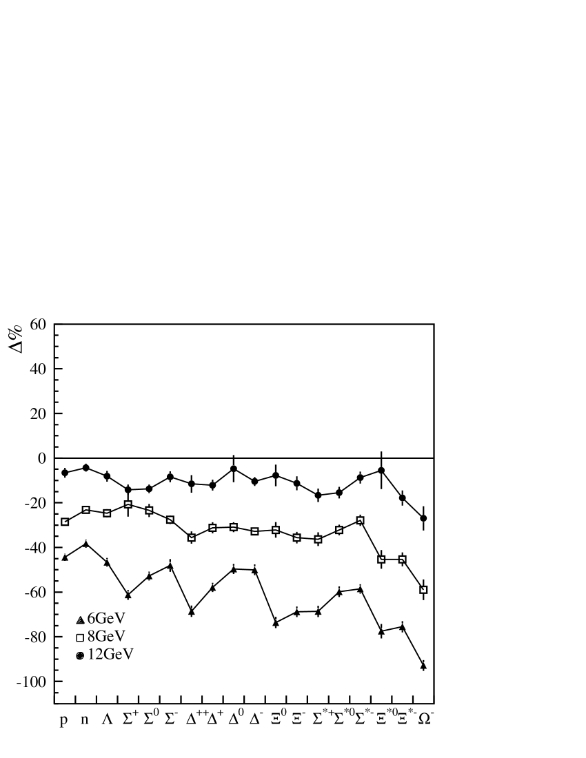
Figure 8: Relative difference between microcanonical and canonical average primary multiplicities of antibaryons $(\langle N_{j}\rangle_{\rm micro}-\langle N_{j}\rangle_{\rm can})/\langle N_{j}\rangle_{\rm can}$ for pp-like clusters with mass 4, 8, 12 GeV. The error bars indicate the statistical error of the importance sampling Monte-Carlo computation. Connecting lines are drawn to guide to eye.

Figure 9: Relative difference between microcanonical and canonical average primary multiplicities of $\pi^{0}$, p and $\Omega$ $(\langle N_{j}\rangle_{\rm micro}-\langle N_{j}\rangle_{\rm can})/\langle N_{j}\rangle_{\rm can}$ for a neutral cluster with mass of 6 GeV as a function of energy density. The error bars indicate the statistical error of the importance sampling Monte-Carlo computation. Connecting lines are drawn to guide to eye.

The relative difference between microcanonical and canonical average for hadrons belonging to basic SU(3) multiplets and three different cluster masses are shown in figs. 4,5,6,7 and 8. At a mass of 4 GeV, the deviation is significant and shows a considerable variation as a function of the species. In neutral clusters, mesons and baryons feature a different behaviour: whilst microcanonical multiplicities of mesons are higher than the corresponding multiplicity in the canonical ensemble, those of baryons are lower. In pp-like cluster, on the other hand, the general behaviour is not as simple; different mesons show different signs of the difference and there are even oscillations of it going from low to high mass clusters. On the other hand, it is evident that already at 8 GeV of mass, where the total primary multiplicity of particles is around 8 (see table 2), all differences between the microcanonical and canonical ensemble do not generally exceed 20% and further shrink to about 10% at 12 GeV. Furthermore, these differences depend only weakly on the energy density, as shown in fig. 9. We can conclude that, as a rule of thumb, the canonical ensemble is a good approximation of the microcanonical one for masses $\gtrsim 8$ GeV at energy densities between 0.1 and 0.9 GeV/fm³ with quantum numbers not greater than that of an elementary colliding system. Provided that the further assumption of the equivalence between the actual set of clusters and an equivalent global cluster (EGC) holds becagp , this result justifies the use of the canonical ensemble in the analysis of particle multiplicities in pp, e⁺e^-and other high energy collisions. Indeed, the mean masses of the EGC corresponding to the actually fitted temperatures and volumes, shown in table 1, turn out to be sufficiently large for most collisions, with the likely exception of K⁺p at $\sqrt{s}=11.5$ GeV and e⁺e^-at $\sqrt{s}=14$ GeV where the mean mass is lower than 7 GeV. At $\sqrt{s}\gtrsim 20$ GeV, the mean mass is larger than 8 GeV, implying that the canonical ensemble is a good approximation.

Table 1: Fitted parameters temperature, volume and extra strangeness suppression parameter ($\gamma_{S}$ or the mean value of produced strange quark pairs out of the vacuum $\langle{\rm s}\bar{\rm s}\rangle$) in elementary collisions in the canonical analysis of hadron abundances. The canonical fit assumes the equivalence, as far as particle multiplicities are concerned, between the set of actual clusters and one global cluster becagp whose resulting mean mass is quoted in the last column. Note that ${\rm e}^{+}{\rm e}^{-}\rightarrow{\rm c}\bar{\rm c}\;$and ${\rm e}^{+}{\rm e}^{-}\rightarrow{\rm b}\bar{\rm b}\;$events, where heavy flavoured hadrons are emitted, have been excluded to estimate $\langle M\rangle$ in e⁺e^-collisions.

Collision	$\sqrt{s}$ (GeV)	Reference	$T$ (MeV)	$V$ (fm3)	$\gamma_{S}$ or $\langle{\rm s}\bar{\rm s}\rangle$	$\langle M\rangle$ (GeV)
K+p	11.5	becagp	176.9$\pm$2.6	8.12$\pm$0.83	$\langle{\rm s}\bar{\rm s}\rangle$= 0.347$\pm$0.020	6.51
K+p	21.7	becagp	175.8$\pm$5.6	12.0$\pm$2.4	$\langle{\rm s}\bar{\rm s}\rangle$= 0.578$\pm$0.056	8.47
$\pi^{+}$p	21.7	becagp	170.5$\pm$5.2	16.7$\pm$3.1	$\langle{\rm s}\bar{\rm s}\rangle$= 0.734$\pm$0.049	8.23
pp	17.2	bgkms	187.2$\pm$6.1	6.79$\pm$1.6	$\langle{\rm s}\bar{\rm s}\rangle$= 0.381$\pm$0.021	7.74
pp	27.4	becagp	162.4$\pm$5.6	25.5$\pm$1.8	$\langle{\rm s}\bar{\rm s}\rangle$= 0.653$\pm$0.017	9.67
e+e-	14	becagp	167.3$\pm$6.5	15.9$\pm$4.1	$\gamma_{S}$= 0.795$\pm$0.088	6.08
e+e-	22	becagp	172.5$\pm$6.7	15.9$\pm$4.8	$\gamma_{S}$= 0.767$\pm$0.094	8.12
e+e-	29	becagp	159.0$\pm$2.6	33.1$\pm$4.0	$\gamma_{S}$= 0.710$\pm$0.047	9.28
e+e-	35	becagp	158.7$\pm$3.4	33.7$\pm$5.2	$\gamma_{S}$= 0.746$\pm$0.040	9.54
e+e-	43	becagp	162.5$\pm$8.1	29.0$\pm$9.2	$\gamma_{S}$= 0.768$\pm$0.065	9.99
e+e-	91.25	becabiele	159.4$\pm$0.8	52.4$\pm$2.2	$\gamma_{S}$= 0.664$\pm$0.014	16.0
${\rm p}\bar{\rm p}\;$	200	becabiele	175$\pm$11	35$\pm$14	$\gamma_{S}$= 0.491$\pm$0.044	21.6
${\rm p}\bar{\rm p}\;$	546	becabiele	167$\pm$11	65$\pm$27	$\gamma_{S}$= 0.526$\pm$0.044	28.7
${\rm p}\bar{\rm p}\;$	900	becabiele	167.6$\pm$9.0	$\simeq 77$	$\gamma_{S}$= 0.533$\pm$0.054	34.8

The quick convergence of microcanonical average multiplicities to canonical ones in a hadron gas is favoured by the large number of available degrees of freedom. From a mathematical point of view, a large number of degrees of freedom makes the saddle point expansion converging faster. In physical terms, there are more ways to conserve energy and momentum in a system with a larger number of particle species, so that fulfilling these constraints become less important earlier than in a system with few degrees of freedom. This is demonstrated in fig. 10 where the relative difference between neutral pion multiplicity in microcanonical and canonical ensemble is shown for a completely neutral pion gas and for a full hadron-gas as a function of cluster mass.

Figure 10: Relative difference between microcanonical and canonical average primary multiplicities of $\pi^{0}$ $(\langle N_{j}\rangle_{\rm micro}-\langle N_{j}\rangle_{\rm can})/\langle N_{j}\rangle_{\rm can}$ a completely neutral cluster and in a pion gas as a function of cluster mass at an energy density of 0.4 GeV/fm³. The error bars indicate the statistical error of the importance sampling Monte-Carlo computation. Connecting lines are drawn to guide to eye.

The microcanonical average multiplicities of most hadrons, to a good approximation, increase linearly as a function of cluster mass, for fixed energy density, starting from $M\simeq 3$ GeV. On the other hand, particles with large charge content (such as $\Omega$) show a stronger dependence on mass, as shown in fig. 11, over the mass range appropriate for microcanonical and canonical calculations.

Figure 11: Microcanonical average primary multiplicities of $\pi^{0}$, p, $\Omega$ and of all hadron species ($h$) in a completely neutral cluster as a function of cluster mass at an energy density of 0.4 GeV/fm³. The error bars indicate the statistical error of the importance sampling Monte-Carlo computation. Lines are drawn to guide to eye.

We have also compared the overall primary multiplicity distributions in the two ensembles. The multiplicity distribution in the microcanonical ensemble has been determined by taking $\delta_{N,\sum_{j}N_{j}}$ as observable in Eqs. (10),(16) and performing an importance sampling Monte-Carlo calculation. The multiplicity distribution in the canonical ensemble has been determined by the same method, that is extracting particle numbers from the MPD and weighing each event fulfilling charge conservation with the ratio between the actual multi-species multiplicity distribution and the MPD. The former reads (see Appendix C):

$$P({{\{N_{j}\}}})=\frac{1}{Z({\bf Q})}$$

$$\times\Bigg{[}\prod_{j}\sum_{\{h_{n_{j}}\}}(\mp 1)^{N_{j}+H_{j}}\prod_{n_{j}=1}^{N_{j}}\frac{z_{j(n_{j})}^{h_{n_{j}}}}{n_{j}^{h_{n_{j}}}h_{n_{j}}!}\Bigg{]}\delta_{{\bf Q},\sum_{j}N_{j}{\bf q}_{j}}$$ (34)

where $\{h_{n_{j}}\}$, as usual, denote partitions and:

$$z_{j(n_{j})}=\frac{(2J_{j}+1)V}{(2\pi)^{3}}\int{\rm d}^{3}{\rm p}\;{\rm e}^{-n_{j}\sqrt{{\rm p}^{2}+m_{j}^{2}}/T}$$ (35)

For $T\approx 160$ MeV, only the leading poissonian terms in the distribution (5) corresponding to $\{h_{n_{j}}\}=(N,0,\ldots)$ can be retained for all particles except pions.

Figure 12: Comparison between microcanonical (solid) and canonical (dashed) overall primary multiplicities distribution in neutral clusters of four different masses at an energy density of 0.4 GeV/fm³.

Figure 13: Comparison between microcanonical (solid) and canonical (dashed) overall primary multiplicities distribution in a pp-like cluster of four different masses at an energy density of 0.4 GeV/fm³.

The comparison between the multiplicity distributions are shown in figs. 12 and 13 for neutral and pp-like clusters respectively. It can be seen that the mean values tend to get closer as mass increases, whilst the dispersion is lower in the microcanonical than in the canonical ensemble, where the distribution is almost poissonian. This remarkable effect on particle number fluctuation is owing to the overall energy-momentum constraint causing a global correlation in particle production. The ratio of the dispersion to the square root of the mean (i.e. the dispersion of a Poisson distribution) tends to a factor 1/2 in the thermodynamical limit (see fig. 14), thus showing that microcanonical ensemble is not equivalent to the grand-canonical ensemble with respect to particle number fluctuations. We are not currently aware of a simple reason of this fact.

Figure 14: Ratio between the dispersion of the microcanonical multiplicity distribution and the square root of its mean in neutral (top) and pp-like (bottom) clusters as a function of mass at an energy density of 0.4 GeV/fm³. Lines are drawn to guide the eye.

Because of the persistence of the shape difference between multiplicity distributions in the two ensembles, the number of channels sampled with the MPD whose weight is much larger than their corresponding microcanonical one increases with total mean multiplicity, hence with cluster’s mass (at fixed energy density). This is the reason of the slightly increasing statistical error on average multiplicities and multiplicity distributions for increasing cluster mass seen in figs. 4,5,6,7,8,12,13. One could remedy this and speed up microcanonical calculations for very large clusters by changing the sampling distribution. For instance, instead of using a MPD to sample individual species numbers, the total number of particles can be first drawn from a gaussian distribution with variance 1/4 of the sum of all hadron primary multiplicities as estimated in the canonical ensemble; then, the number of baryons $N_{B}$, strange mesons $N_{S}$, charged non-strange mesons $N_{Q}$, neutral mesons $N_{0}$ and their respective number of antiparticles could be sampled from a multinomial distribution:

$$P=N!\prod_{i=1}^{7}\frac{\xi_{i}^{N_{i}}}{N_{i}!}$$ (36)

where $i=B,{\bar{B}},S,{\bar{S}},Q,{\bar{Q}},0$ and $\xi_{i}$ are the sums of all $\nu_{j}$ functions in Eq. (21) of particles belonging to the same class $i$. Finally, once the multiplicities of each class $N_{i}$ fulfilling conservation laws have been extracted, individual particle multiplicities could be determined for each class in turn by using again multinomial distributions.

Table 2: Mean multiplicity $\langle N\rangle$ and dispersion $D$ of the microcanonical and canonical multiplicity distribution for neutral and pp-like clusters as a function of the mass. Also quoted the corresponding temperature in the canonical ensemble obtained from Eq. (31).

Neutral cluster
	Microcanonical		Canonical
$M$ (GeV)	$\langle N\rangle$	$D$	$\langle N\rangle$	$D$	$T$ (MeV)
2	2.43	0.63	1.96	1.74	175.3
4	4.45	1.01	4.08	2.45	169.3
6	6.53	1.24	6.17	2.93	166.3
8	8.61	1.43	8.27	3.29	164.6
10	10.67	1.59	10.38	3.58	163.5
12	12.76	1.75	12.46	3.90	162.8
14	14.84	1.89	14.56	4.15	162.2
pp-like cluster
	Microcanonical		Canonical
$M$ (GeV)	$\langle N\rangle$	$D$	$\langle N\rangle$	$D$	$T$ (MeV)
4	3.87	0.81	3.63	1.33	142.1
6	6.04	1.08	5.76	2.05	152.5
8	8.20	1.30	7.90	2.59	156.1
10	10.35	1.49	10.04	3.02	157.8
12	12.48	1.66	12.17	3.40	158.7
14	14.60	1.82	14.27	3.73	159.2

6 The Metropolis algorithm

The importance sampling method allows to calculate averages like (10) in single Monte-Carlo runs quite straightforwardly and can be used as an event generator if events are reweighted, as we have seen, by a factor $\Omega_{\{N_{j}\}}/\Pi_{\{N_{j}\}}$. If one needs to sample $\Omega_{\{N_{j}\}}$ directly without reweighting the events, different methods should be considered. A first possibility is a rejection method, but it can be soon realized that it is unfit for the problem we are dealing with. In fact, for this method to be effective, one needs a covering function $F({\{N_{j}\}})$ (i.e. a function of the channel such that $F({\{N_{j}\}})>\Omega_{\{N_{j}\}}\;\forall{\{N_{j}\}}$ which can be sampled very efficiently and as close as possible to the $\Omega_{\{N_{j}\}}$. Such a function is hard to find because $\Omega_{\{N_{j}\}}$ is not smooth in its domain; strong variations of the phase space volume may occur by changing just one particle. We have seen that the MPD is likely to be similar to our target distribution, but in order to be a covering function, it should be rescaled by a factor $c$ such that $c\Pi_{\{N_{j}\}}>\Omega_{\{N_{j}\}}\;\forall{\{N_{j}\}}$. However, to estimate $c$, one ought to evaluate $\Omega_{\{N_{j}\}}$ for all channels and this is just what cannot be afforded. A general method to sample complex multi-dimensional distributions is the Metropolis algorithm metro , which has been applied to the specific problem of numerical calculations of the multihadronic microcanonical ensemble by Werner and Aichelin weai . In this work, we will show that this method can be further improved in speed and accuracy and, at the same time, that great care is needed in handling it, especially when assessing the equilibrium conditions.

The Metropolis algorithm prescribes the implementation of a random walk in the channel space on the basis of acceptance or rejection of proposed transitions from the current position. After some number of steps, the probability of visiting a given point is proportional to the target distribution; otherwise stated, the points in the random walk are actual samples of the the target distribution (in our case $\Omega_{\{N_{j}\}}$) and they can be stored as generated events. We will now discuss more in detail how this comes about. In a general random walk, the probability $P_{m}(t)$ of visiting a state $m$ (i.e. a channel or multi-hadronic configuration) at the $t^{\rm th}$ step evolves according to the master equation:

$$P_{m}(t+1)-P_{m}(t)=\sum_{n}P_{n}(t)w(n\rightarrow m)-P_{m}(t)w(m\rightarrow n)$$ (37)

where $w(n\rightarrow m)$ is the probability of transition from the state $n$ to the state $m$. At the equilibrium:

$$P_{m}(t+1)=P_{m}(t)\qquad\forall m$$ (38)

This occurs if (a sufficient but not necessary condition):

$$P_{n}(t)w(n\rightarrow m)=P_{m}(t)w(m\rightarrow n)\qquad\forall n,m$$ (39)

If we want the probabilities $P_{m}$ to be proportional to a given target distribution $f(m)$, so that the number of times the state $m$ is visited from some step $t$ onwards is proportional to $f(m)$, we have to enforce the condition:

$$\frac{w(n\rightarrow m)}{w(m\rightarrow n)}=\frac{f(m)}{f(n)}\;.$$ (40)

Provided that the above equation is fulfilled, the choice of a set of transition probabilities $w$ (a so-called updating rule), is free. The only requirement is that every point can be reached from any point in a finite number of steps with non-vanishing probability (ergodicity condition), otherwise there would be unaccessible regions even though $f\neq 0$ therein. Although any choice of the $w$’s is in principle allowed, some are worthier. Indeed, the transition probabilities $w$ govern the dynamical behaviour of the random walk and, particularly, how fast the system gets to the equilibrium condition (38) after a transient. This is owing to the fact that, in general, the random walk starts from states which are not random samples of the target distribution, so that $P_{m}(0)\neq f(m)$. A good choice of the $w$’s will keep the relaxation time $T_{rel}$, defined as the number of steps needed to get sufficiently close to the equilibrium value, to a minimum, thereby making event generation faster.

In general, the transition probability can be decomposed into a proposal probability $T$ (proposal matrix), i.e. the probability of considering a given transition, and the conditional probability $A$ of accepting it once it has been proposed. In symbols:

$$w(n\rightarrow m)=T(n\rightarrow m)A(n\rightarrow m)\;.$$

Starting from a non-equilibrium situation, a physical system reaches equilibrium earlier if transition probabilities are larger. Likewise, in the Metropolis algorithm, the relaxation time is little if $w(n\rightarrow m)$ are large; in other words, if $w(n\rightarrow n)$ is small taking into account the normalization condition:

$$\sum_{m}w(n\rightarrow m)=1$$ (41)

For the transition probabilities to states different from the current state to be large, the acceptance matrix should be as large as possible for $m\neq n$ once the proposal matrix is known. There is indeed an optimal choice for $A$ which reads:

$$A(n\rightarrow m)=\min\Bigg{\{}1,\frac{f(m)T(m\rightarrow n)}{f(n)T(n\rightarrow m)}\Bigg{\}}\;.$$ (42)

This choice maximizes $w(n\rightarrow m)$ if $n\neq m$ umri and fulfills the condition (40). The next problem is choose a good proposal matrix. The issue is discussed in detail in ref. umri and the conclusion is that $T(n\rightarrow m)\simeq f(m)$, i.e. the proposal matrix should be an easy-to-sample distribution as close as possible to the target distribution $f(m)$. This can be easily understood by taking the limiting case (which, if possible, would make the Metropolis algorithm unnecessary):

$$T(n\rightarrow m)=f(m)$$ (43)

In this case, the relaxation time would be zero: the starting point, as well as all other points in the random walk, would be sampled from the target distribution itself and any transition would be accepted because $A(n\rightarrow m)=1$ according to Eqs. (42) and (43). While the condition (43) cannot be obtained in practice (Metropolis algorithm would be unnecessary in that case), one can try to get as close as possible to it. From what we have seen in Sect. 4 about importance sampling, it can be argued that the MPD in Eq. (20) would be a good proposal matrix and could also be used to pick the starting point in the Metropolis random walk. We will see the benefits of the use of the MPD more in detail in the next section.

A drawback of the Metropolis algorithm is that, unlike in the importance sampling method, different samples (i.e. steps in the random walk) are not independent. This can be easily understood reminding that proposed transitions may be rejected, so that a point may appear several times in a row in the random walk. Hence, there is a finite positive statistical correlation between the values of physical observables at different steps and this gives rise to an increase of the overall uncertainty in the estimate of averages with respect to the case of independent samples. The fact that different events are correlated may render the use of Metropolis algorithm not appropriate in some applications. However, in the problem of high energy collision event simulation, where one has to hadronize many clusters with different masses in each event, this is not an issue; in this case, a single Metropolis random walk must be run for each cluster, and only one sample, representative of its microcanonical ensemble, drawn after equilibrium has been reached.

The Metropolis algorithm can be used to estimate the average of an observable like (10) in the microcanonical ensemble of a single cluster by taking a sufficiently large number of steps (i.e. $\gg T_{rel}$) in one random walk and calculating:

$${\langle O\rangle}\doteq\frac{\sum_{k=1}^{M}O^{(k)}}{M}$$ (44)

where $M$ is the total number of steps and $O^{(k)}$ the actual value of the observable $O$ at $k^{\rm th}$ step. A nice feature of the Metropolis algorithm is that, unlike in the importance sampling method, there is no need of overall normalization when estimating ${\langle O\rangle}$ (compare Eq. (44) with Eq. (17)). On the other hand, as already emphasized, the values of $O$ at different steps are correlated. The statistical error on ${\langle O\rangle}$ in Eq. (44) can be estimated as (see Appendix D):

$$\sigma_{\langle O\rangle}=\sqrt{\frac{\langle O^{2}\rangle-{\langle O\rangle}^{2}+2R}{M}}$$ (45)

where $R$ is the integral of the autocorrelation function $A$, defined here as the difference between the expectation value of the product of the observable value at the steps $k$ and $k+h$ and its average $\langle O\rangle^{2}$

$$A(h)\equiv{\sf E}({\sf O}^{(k)}{\sf O}^{(k+h)})-\langle O\rangle^{2}$$ (46)

If the starting point is random, the autocorrelation function is independent of $k$ and gives information about how correlated are distant steps, namely how long the system keeps memory of its past steps. As already mentioned, this correlation between different steps arises from the finite probability of rejecting transitions and vanishes only if all proposed transitions are accepted, i.e. if Eq. (43) is fulfilled. Therefore, the autocorrelation function is always positive and vanishes only if different steps are independent. Moreover, the statistical error (45) is larger than in the case of uncorrelated samples, where it reaches its minimum. The number of steps needed to reduce $A(h)$ to some small fraction of ${\langle O\rangle}^{2}$ is defined as autocorrelation time $T_{auto}$. Thus, in order to minimize the statistical error on ${\langle O\rangle}$ in Eq. (45), one should keep the autocorrelation time as little as possible.

The autocorrelation function and time depend only on the updating rule, whilst the relaxation time $T_{rel}$ also depends on how the initial state is chosen. In principle, the relaxation time might be zero while the autocorrelation time is not. When using the MPD both as proposal matrix and to generate the starting point, these two quantities are tightly related.

The autocorrelation function can be estimated during the Metropolis random walk by the sum:

$$A(h)\doteq\frac{\sum_{k=1}^{M-T_{auto}}O^{(k)}O^{(k+h)}}{M-T_{auto}}-\frac{1}{M^{2}}\left(\sum_{k=1}^{M}O^{(k)}\right)^{2}$$ (47)

and it is shown in fig. 15 for a cluster of 4 GeV with updating rule based on the MPD.

Now the question arises whether the Metropolis algorithm leads to more or less accurate computations of mean values than the importance sampling method, for given computing resources and using the same distribution $\Pi_{\{N_{j}\}}$ as proposal matrix and sampling distribution respectively. This is studied in more detail in Subsect. 7.4.

Figure 15: Autocorrelation function for the total primary multiplicity for a neutral cluster of 4 GeV mass at an energy density of 0.4 GeV/fm³.

7 Study of the Metropolis algorithm

We have studied the capability of the Metropolis algorithm as an event generator for the statistical model of hadronization and as a computing tool for the hadron gas microcanonical ensemble. As has been discussed in the previous section, the benchmark for this algorithm is the number of steps needed to reach equilibrium, or relaxation time $T_{rel}$, which must be kept to a minimum so as to draw samples of the target distribution as quickly as possible. Likewise, the autocorrelation time $T_{auto}$ must be small in order to minimize the statistical error (45) on the estimate of mean values in single random walks. As has been mentioned at the end of previous section, these two quantities are tightly related in our MPD-based scheme, so we can confine ourselves to study $T_{rel}$.

The relaxation time in principle depends on the physical observable (average multiplicities, multiplicity distribution etc.) and it is not easy to estimate in advance. Hence, in practice, it must be determined a posteriori by analyzing the convergence to equilibrium for the observable of interest. For instance, if we ought to calculate the overall multiplicity distribution $P_{n}$, we would have to study the height of the $n^{\rm th}$ bin, for all $n$’s, as a function of the step. The height of the $n^{\rm th}$ bin at the $k^{\rm th}$ step, that is $P_{n(k)}$, can be estimated by repeating the Metropolis random walk many times and averaging:

$$P_{n(k)}=\frac{1}{L}\sum_{i=1}^{L}\delta_{n,n_{i(k)}}$$ (48)

where $n_{i(k)}$ is the actual multiplicity in the $i^{\rm th}$ random walk at the step $k$.

Establishing when a stable value of the examined observable is attained can be done by studying its average over many Metropolis random walks, like (48) as a function of the step, i.e. forming a hystogram (the step hystogram, see fig. 16) with Metropolis step numbers as bins and the average of the observable (e.g. multiplicity) as bin content. In all considered cases, the step hystogram shows the same general behaviour, namely a tendency to an equilibrium value after, possibly, a strong initial oscillation and followed, sometimes, by very mild damped oscillations. Step hystograms show fluctuations around an apparent equilibrium value at some scale, as it can be seen in figs. 16,17. The fluctuation pattern is determined by the interplay of finite statistics and possible dynamical oscillations governed by the master equation (37). The amplitude of statistical fluctuations is a function of the updating rule.

Figure 16: Step hystogram showing the convergence to equilibrium of the probability $P_{7}$ of a channel with 7 primary hadrons as a function of the step in a set of 500000 Metropolis random walks for a neutral cluster of 6 GeV with energy density of 0.4 GeV/fm³. The horizontal solid line indicates the $P_{7}$ value estimated with the importance sampling method and the dashed band its relevant statistical uncertainty. The arrow points to the equilibrium point determined through the WOSSR test (see text).

Because of these facts, providing a good quantitative assessment of where stability is achieved is not straightforward. Were the statistics of Metropolis random walks infinite, the criterium for stability would be fully deterministic, that is based on the relative difference between asymptotic value (the true microcanonical average) and actual value from a given step onwards. On the other hand, we can only deal with finite statistics, so the estimation of a stability point (thence $T_{rel}$) for a given observable can be done statistically, thus it will be affected by some uncertainty.

The statistical method we have chosen in order to assess the convergence to equilibrium is based on a non-parametric statistical test, the Wilcoxon one sample signed rank test (WOSSR), that we will shortly describe in the following. The WOSSR test is a non-parametric test, i.e. it does not require the knowledge of the statistical distribution of the sample, and the hypothesis under test (the null hypothesis) is that a set of $M$ independent random samples $\{x_{1},\ldots,x_{M}\}$ has a given median $X_{m}$. The only requirement is that their distribution is symmetric. The test procedure consists in sorting the absolute values of the differences $d_{i}=x_{i}-X_{m}\;\;\forall i$ and giving them a rank, namely 1 to the largest, 2 to the second largest and so on. If $X_{m}$ is a good median, the sum of the ranks of the positive differences is expected to be close to the sum of the ranks of negative differences. The test statistic is just the sum $W$ of the ranks of the positive differences and the test result is good when $W$ is close to half the sum of the first $M$ integers, that is $M(M+1)/4$.

We have used this method to study the convergence to equilibrium in the Metropolis algorithm taking as random samples a subset of $M$ running bins (from the $k^{\rm th}$ to the $(k+M)^{\rm th}$) in the step hystogram of the multiplicity distribution $P_{n(k)}$ (see fig. 16). In fact, if equilibrium is reached in the Metropolis random walk (as it is apparent in the rightmost part of the hystogram in fig. 16), $P_{n(k)}$ is expected to evenly fluctuate around the asymptotic equilibrium value, whereas a net drift towards this value appears when out of equilibrium (i.e. in the leftmost part of fig. 16). Therefore, provided that the distribution of fluctuations is symmetric at equilibrium, the asymptotic value is likely to be a good median for sets of $P_{n(k)}$ with $k=1,\ldots,M$ in the equilibrium region and not in the drifting region. Accordingly, the WOSSR test will yield a good confidence level in the former case and a very small one in the latter. The true asymptotic value is not known in practice and must be estimated from the step hystogram itself. A good choice is the arithmetic mean of a set of hystogram contents in the rightmost region, where stability is apparently reached.

The non-parametric WOSSR test carried out on a set of $M$ running bins in the step hystogram seems suitable for our problem. In fact, we do not know the statistical distribution of the random variable ${\sf O}^{(k)}$ (i.e. the examined observable) at each step for a given number $L$ of random walks. On the other hand, it is reasonable to assume that it is symmetric at equilibrium around the asymptotic value which is one of the requirement of the WOSSR test. However, this test also requires the independence of samples, which is not the case here because subsequent steps in Metropolis random walks are indeed correlated, as has been emphasized. Thus, the results of WOSSR test in this context should be taken with much care and could be misleading if $M\ll T_{auto}$. If a large fluctuation from equilibrium value occurs at some point, its persistency in sign is fed by the positive correlations of adjacent points and this will drive the test to failure even if equilibrium was actually achieved. Conversely, it is quite unlikely that the test yields a positive answer on a sufficiently large set of running bins if equilibrium is not achieved, unless two accidentally large fluctuations of equal time size arise. Therefore, albeit not appropriate in principle, the WOSSR test with $M\sim T_{auto}$ provides a fairly good indication of equilibrium.

In order to actually define an equilibrium point, and thereby a relaxation time $T_{rel}$, we first calculate the arithmetic mean of the rightmost 50 (which is of the same order as of $T_{auto}$) bin contents, which is taken as median $X_{m}$ to be fed in the test. The WOSSR test is then performed on subsets of $M=10$ running bins in the step hystogram taking as starting bin the leftmost and moving rightward by one bin at a time. The test is regarded as successful if it yields a confidence level of at least 0.05 for a median differing from the previously defined $X_{m}$ at most by 0.5%. If the test is successful for 10 starting bins in a row, the first of those ten is taken to be the equilibrium point. Little variation of the equilibrium point is found by changing the number of running bins from 5 to 20.

Henceforth, we will use the observable overall multiplicity and WOSSR test to point out some important features of the Metropolis algorithm.

7.1 Dependence on the integration method

It has been shown in Sect. 4 that the importance sampling integration method benefits from drawing samples in the extended space of the variables:

$$\{N_{1},\ldots,N_{K}|r_{1},\ldots,r_{N-1}\}\qquad{\rm with}\;\;N=\sum_{j}N_{j}$$ (49)

instead of calculating the integral in the $r$’s for each channel ${\{N_{j}\}}$ in Eq. (4) with a fixed (say 1000) number of Monte-Carlo samples. One could try to apply the same idea to the Metropolis algorithm: instead of making a random walk in the space of channels ${\{N_{j}\}}$ and evaluating the weight of the channel at each step by performing a Monte-Carlo integration of $\Omega_{\{N_{j}\}}$ in Eq. (4), samples can be drawn in the extended space of the above variables and evaluating the integrand function $\Psi$ only one time at each step, thus saving CPU time. However, the relaxation time $T_{rel}$ will be different in these two cases and most likely longer in the extended space sampling case. This can be easily understood if the single $\Psi$ evaluation is regarded as the extreme approximation of the integral in the $r$’s in Eq. (4) with $N_{S}=1$. This is shown indeed in fig. 17: the convergence to the equilibrium speeds up if the number of samples used to estimate the integral in Eq. (4) increases. A serious drawback of the extended space sampling, i.e. with $N_{S}=1$, is that the relaxation time may become so long that many bins of the multiplicity distribution look like having reached their stable asymptotic value even when they actually still slowly drift towards it. We have checked this for the case shown in fig. 17 by pushing the Metropolis random walk to 10000 steps, much beyond the scale of the step hystogram. It has been found that even at such large number of steps, the asymptotic value, calculated independently with the importance sampling method, is not attained, though the WOSSR test yields a positive response, under most circumstances. This finding indicates that the use of Metropolis algorithm requires more care than expected. At least a comparison between the apparent asymptotic stable values with different number of samplings or a cross-check with independent calculations is necessary.

Figure 17: Step hystogram showing the convergence to equilibrium of the probability $P_{6}$ of a channel with 6 primary hadrons as a function of the step in a set of 500000 Metropolis random walks for different numbers of samples $N_{S}$ in the Monte-Carlo integration of the phase space volume of each channel $\Omega_{\{N_{j}\}}$ in Eq. (4). The horizontal solid line indicates the $P_{6}$ value estimated with the importance sampling method and the dashed band its relevant statistical uncertainty. Cluster mass is 8 GeV, energy density 0.4 GeV/fm³ and charges are free.

7.2 Dependence on the updating rule

In order to show the effectiveness of the updating rule based on randomly sampling the MPD, as discussed in Sect. 4, we have compared it with a simpler updating rule based on milder changes of the current configuration. This rule is as follows:

1. Three probabilities $\eta_{0}$, $\eta_{+}$ and $\eta_{-}$ are chosen such that $\eta_{0}+\eta_{+}+\eta_{-}=1$.

2. A random extraction $(0,+,-)$ is made according to the probability distribution defined by the $\eta$’s.

3. Depending on whether the outcome is $0,+,-$ the overall number of particles in the configuration is kept, is increased by 1 unit or decreased by 1 unit respectively. In the first case, a randomly chosen particle in the current configuration is replaced with one having a mass just above or below. In the second case, a new particle is randomly chosen among all possible species. In the third case, a randomly chosen particle of the current configuration is removed.

For this updating rule, the proposal matrix $T(m\rightarrow n)$ has been determined and optimal acceptance matrix set accordingly (see Eq. (42)).

Indeed, this rule involves a slowing down of the convergence to equilibrium because the fraction of rejected transitions is much higher than in the MPD-based updating rule. This is apparent in fig. 18 where the relevant step hystograms are shown for the multiplicity distribution bin with 2 particles for a 2 GeV mass cluster. Whilst in the MPD-based updating rule the equilibrium is achieved within few tens of steps, in the above rule stability is not achieved even after 3000 steps. Similar differences are found for heavier clusters. Therefore, the MPD-based updating rule is much more efficient with regard to computing time.

Figure 18: Step hystogram showing the convergence to equilibrium of the probability $P_{2}$ of channels with 2 hadrons as a function of the step in a set of 100000 Metropolis random walks for the updating rule based on the MPD (bottom) and on a simpler method described in the text (top). Solid lines indicate the true value obtained by computing the phase space volume of all of the channels. The cluster mass is 2 GeV, the energy density 0.4 GeV/fm³ and charges are free. The number of samples used in the numerical integration of Eq. (4) was $N_{S}=1000$. For this comparison, resonances have been kept at a fixed mass and quantum statistics terms in $\Omega_{\{N_{j}\}}$ have been neglected.

7.3 Dependence on the cluster mass and charge

We have studied the dependence of $T_{rel}$ on the cluster mass and charges, at constant energy density, by applying the WOSSR tests to step hystograms of multiplicity distribution $P_{n}$ in different bins. For each mass and set of charges we have taken the highest $T_{rel}$ among the bins for which $P_{n}>10^{-3}$, as $the$ relaxation time for that cluster. This study has been carried out for completely neutral and pp-like clusters; energy density has been kept constant at 0.4 GeV/fm³. For each cluster 500000 Metropolis random walks (100000 for $M=10$ GeV) have been performed up to 300 steps. The relaxation times are shown in fig. 19.

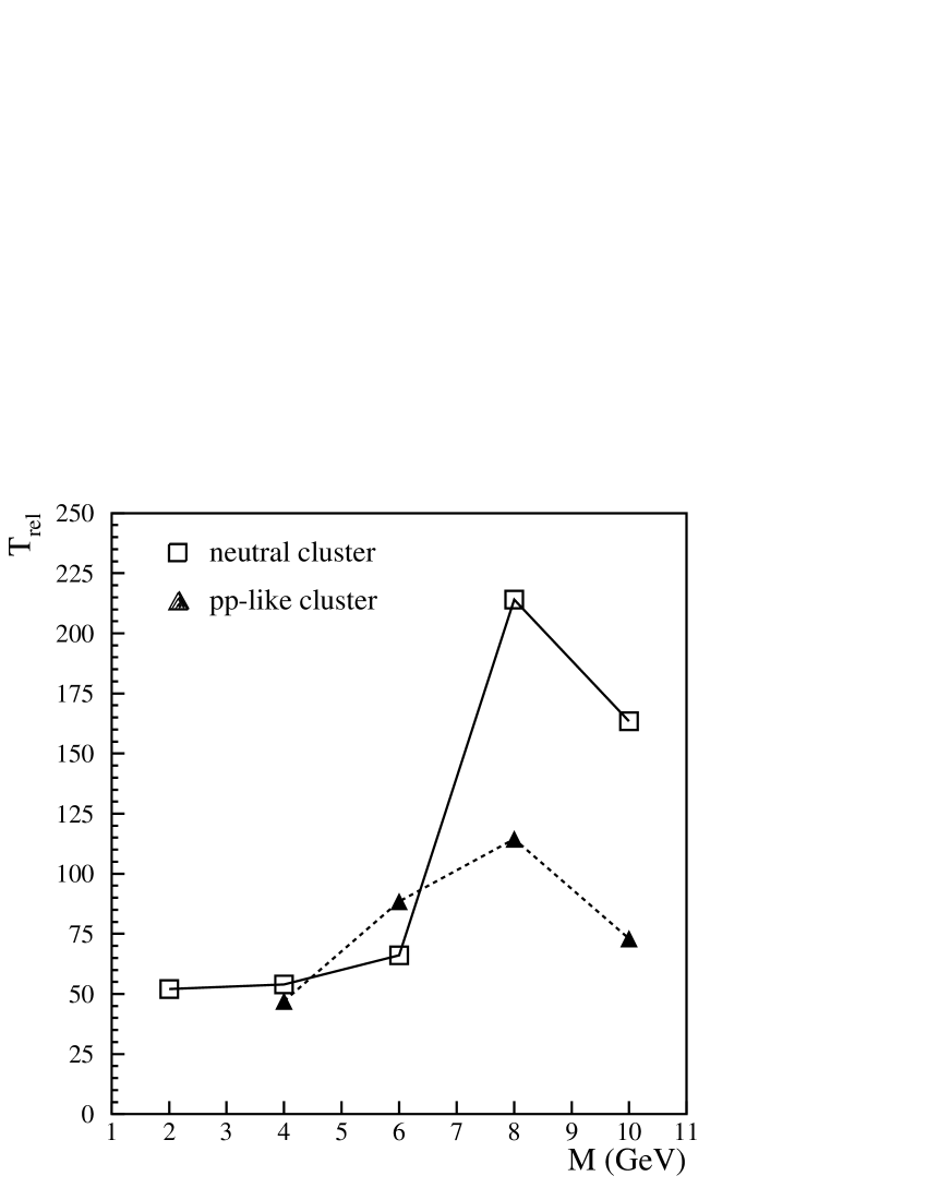
Figure 19: Relaxation times in a Metropolis random walk (see text for the definition) as a function of mass and charges of the cluster. Energy density is kept fixed at 0.4 GeV/fm³. Lines are drawn to guide the eye.

This just defined relaxation time shows an initial increase as a function of the cluster mass and drops thereafter going from 8 to 10 GeV. For the present, we do not have a complete understanding of this behaviour. An increase as a function of the mass is expected because the number of channels sampled from the MPD whose weight is much larger than their correspoding microcanonical one increases owing to the persistence of the shape difference between multiplicity distributions in the canonical and microcanonical ensemble (see figs. 12,13), as already mentioned in Sect. 5. The drop, as well as the observed difference between neutral and pp-like cluster, in the region 8-10 GeV might be a genuine effect due to a local minimal distance between MPD and microcanonical distributions or an artefact of the cut on probability at $10^{-3}$. What it is important to remark is that the relaxation times are not larger than ${\cal O}(100)$ in the region where microcanonical calculations are necessary. In order to further improve Metropolis calculations, the same modification of the sampling distribution put forward at the end of Sect. 4 to reduce statistical error in the importance sampling, could be carried over here so as to speed up the convergence to equilibrium.

7.4 Comparison with the importance sampling method

The performances of importance sampling method and Metropolis algorithm have been compared by studying the statistical error on the calculation of averages of several observables with the same computing resources. For a neutral cluster with 4 GeV mass and 0.4 GeV/fm³ energy density, we have calculated the total average multiplicity and the primary multiplicity distribution 100 times, each time taking 100000 steps in both methods. As the sampled distribution at each step is the MPD in both cases, the used CPU time is approximately the same. The function $\Psi$ in Eq. (4) has been sampled one time per channel in both methods.

As an example, we show in fig. 20 the results obtained for the estimate of the probability $P_{5}$ of channels with 5 primary hadrons. It can be seen that the Metropolis algorithm gives rise to a broader statistical distribution of the estimated values with respect to the importance sampling method. Moreover, the distribution is not gaussian and it is slightly asymmetric with also few cases of outranging estimates. On the other hand, the distributions for the total average multiplicity look quite similar in the two methods. It is worth pointing out that the a priori statistical error estimate obtained by using Eq. (18) for the importance sampling method is about 0.008, in good agreement with the found RMS of 0.0087 quoted in fig. 20.

We have not investigated in much detail the sources of such a different statistical resolution, but we surmise that the ultimate reason of a larger error in Metropolis algorithm is the extra call to the random number generator which, at each step, is possibly needed to accept or reject a proposed transition. Ultimately, this is an additional source of fluctuations in the Metropolis random walk which is absent in the importance sampling method where each extracted configuration is simply reweighted. Altogether, the importance sampling method seems to be better performing to calculate averages in the microcanonical ensemble.

Figure 20: Statistical distribution of the Monte-Carlo estimates of the probability $P_{5}$ of channels with 5 primary hadrons, for a neutral cluster with 4 GeV mass and 0.4 GeV/fm³ energy density.

8 Conclusions

We have calculated averages in the microcanonical ensemble of the ideal hadron-resonance gas including all light-flavoured known resonances up to a mass of about 1.8 GeV. We have found that microcanonical average multiplicities of different hadron species differ by less than 10% from the corresponding canonical average (i.e. calculated by introducing a temperature) for clusters with relatively low mass, around 8 GeV, and energy density of 0.4 GeV/fm³. This confirms and extends previous findings liu obtained with a restricted sample of hadron species. However, multiplicity distributions in the two ensembles show a clear difference in shape which seem to persist in the thermodynamical limit. Particularly, the dispersion of the total multiplicity distribution is, to a great accuracy, 1/2 of the Poisson dispersion in the large volume limit; presently, we do not have any simple explanation of this fact and whether this is linked to our special choice of the energy density.

A major point of this study is concerned with the numerical methods developed to calculate microcanonical averages: an importance sampling method, which has been proposed and used in this work for the first time; and a previously proposed Metropolis algorithm weai , whose performances have been improved by using as proposal matrix Poisson distributions with mean values set as those of the grand-canonical ensemble. They have been also employed as sampled distributions in the importance sampling method.

The Metropolis algorithm is capable to provide single samples of the microcanonical ensemble with unit weight and it is thus a suitable tool for event generation. Yet, it was proved to be less accurate than the importance sampling method for the calculation of averages for single clusters. Moreover, the Metropolis algorithm used for event generation requires much care, particularly a preliminary study of how fast the equilibrium condition is achieved. The convergence to equilibrium may depend on the observable to be analyzed and, more worrying, on the specific integration methods to evaluate the microcanonical weights of the channels.

However, the present study indicates that there is still room for a further improvement of the efficiency of both examined methods. An efficient way of calculating microcanonical ensemble opens the way to test the statistical hadronization model at low energy and with respect to many more observables than those considered as yet.

Appendix

Appendix A Calculation of the phase space integrals

Here we summarize a method to calculate phase space integrals due to Hagedorn cerhag1 . An analytical calculation of $\Phi$ in Eq. (12) can be carried out for two or three particles whilst for more particles the expressions get rapidly so complicated that a numerical computation is much more suitable.

For two particles:

$$\Phi(M,m_{1},m_{2})=\frac{4\pi{\rm p}^{*}}{T^{2}}\frac{\epsilon_{1}\epsilon_{2}}{M}$$ (A.1)

where $m_{i}$’s are the masses, $\epsilon_{i}=\sqrt{{\rm p}^{*2}+m_{i}^{2}}$ the energies, $M$ the cluster’s mass, $T$ the total available kinetic energy and:

$${\rm p}^{*}=\frac{1}{2}\bigg{[}M^{2}-2(m_{1}^{2}+m_{2}^{2})+\frac{1}{M^{2}}(m_{1}^{2}-m_{2}^{2})^{2}\bigg{]}^{\frac{1}{2}}.$$ (A.2)

For $N>2$ a function $W$ of the momenta ${\rm p}_{1},\ldots,{\rm p}_{N}$ is introduced:

$$\Phi=\frac{(4\pi)^{N}}{T^{3N-4}}\int\Big{[}\prod_{i=1}^{N}{\rm d}{{\rm p}}_{i}\;{{\rm p}}_{i}^{2}\Big{]}\,\delta(M-\sum_{i=1}^{N}{\epsilon}_{i})\,W({\rm p}_{1},\ldots,{\rm p}_{N})$$ (A.3)

The function $W$ reads:

$$W({\rm p}_{1},\ldots,{\rm p}_{N})=\frac{1}{(4\pi)^{N}}\int\biggl{[}\prod_{i=1}^{N}{\rm d}\Omega_{i}\biggr{]}\;\delta^{3}(\sum_{i=1}^{N}{\rm p}_{i}\hat{\bf p}_{i})$$ (A.4)

where $\hat{\bf p}_{i}={\bf p}_{i}/{\rm p}_{i}$, and can be calculated explicitely:

$$\!\!\!\!\!\!\!\!\!\!W({\rm p}_{1},\ldots,{\rm p}_{N}) = -\frac{1}{2^{N+1}\pi(N-3)!{\rm p}_{1}\ldots{\rm p}_{N}}$$ (A.7)

$$\times \!\!\!\!\!\sum_{\begin{array}[]{ll}{\scriptstyle\{\sigma_{1}\ldots\sigma_{N}\}}\\ {\scriptstyle\sum\sigma_{j}{\rm p}_{j}\geq 0}\end{array}}\sigma_{1}\ldots\sigma_{N}\big{(}\sum_{i}\sigma_{i}{\rm p}_{i}\big{)}^{N-3}$$

where $\sigma$ can be either $+1$ or $-1$. This expansion involves a large number of terms even at relatively small $N$, so it is more advantegeous under some circumstances, to calculate $W$ differently. In fact, one can set in Eq. (A.4):

$$\delta^{3}(\sum_{i=1}^{N}{\rm p}_{i}\hat{\bf p}_{i})=\frac{1}{(2\pi)^{3}}\int{\rm d}^{3}{{\rm u}}\;\exp\big{[}-{\rm i}\sum_{i=1}^{N}{\rm p}_{i}\hat{\bf p}_{i}\cdot{\bf u}\big{]}$$ (A.8)

which leads to weai :

$$W({\rm p}_{1},\ldots,{\rm p}_{N})=\frac{1}{2\pi^{2}}\int_{0}^{\infty}{\rm d}{\rm u}\;{\rm u}^{2}\prod_{i=1}^{N}\frac{\sin({\rm p}_{i}{\rm u})}{{\rm p}_{i}{\rm u}}$$ (A.9)

Setting now $y={\rm u}\mu$, where $\mu$ is an arbitrary energy scale, to make integration variable adimensional:

$$W({\rm p}_{1},\ldots,{\rm p}_{N})=\frac{1}{2\pi^{2}\mu^{3}}\int_{0}^{\infty}{\rm d}y\;y^{2}\prod_{i=1}^{N}\frac{\sin[({\rm p}_{i}/\mu)y]}{({\rm p}_{i}/\mu)y}$$

$$=\frac{1}{2\pi^{2}\mu^{3}}\int_{0}^{1}{\rm d}x\;\frac{(1-x)^{N-4}}{x^{N-2}}\prod_{i=1}^{N}\frac{\sin\left(\frac{{\rm p}_{i}}{\mu}\frac{x}{1-x}\right)}{p_{i}/\mu}$$ (A.10)

where the last expression has been obtained by using the variable transformation $y=x/(1-x)$. The last integral can be calculated numerically provided that the number of particles is at least of the order of 10, otherwise the integrand function features strong oscillations which make most numerical integration methods failing. In this case, it is compelling to calculate $W$ by means of its full expansion (A.7). However, the CPU time needed to sum all of the terms rapidly grows with $N$, so that for $N>10$ it is definitely preferrable to switch to the numerical computation of the integral (A) (see also fig. 2). The arbitrary scale $\mu$ can be set so as to obtain a good resolution in the numerical computation of $W$ and we have found that $\mu=1$ GeV is an appropriate choice for most cases at the energy densities we have been dealing with; if the number of momenta larger than 100 MeV is $\leq 10$, we set $\mu=100$ MeV.

In order to minimize the CPU time spent to calculate $W$ by using its full expansion (A.7) we have optimized the loop over all combinations $\{\sigma_{1},\ldots,\sigma_{N}\}$ such that $\sum\sigma_{j}{\rm p}_{j}>0$ by considering only those which are relevant. The momenta ${\rm p}_{1},\ldots,{\rm p}_{N}$ are first sorted such that ${\rm p}_{1}>{\rm p}_{2}>\ldots>{\rm p}_{H}$ and all possible $N$-uples made of $+1$ or $-1$ are arranged in a multi-level tree structure shown in fig. 21 for the special case $N=4$.

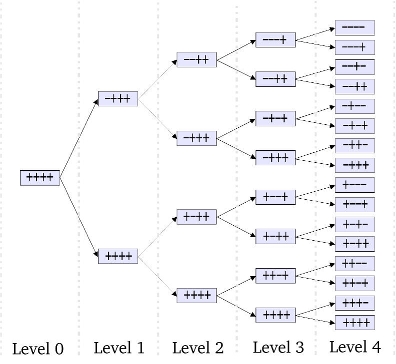
Figure 21: Tree diagram to calculate $W$ with (A.7) for 4 particles.

If, for some $N$-uple at some level $\sum_{j=1}^{H}\sigma_{j}{\rm p}_{j}\leq 0$, the same is true for all $N$-uples branching from it because of momentum sorting and of the tree structure, which is such that moving upwards one level a change in sign $(+\rightarrow-)$ occurs. Note that replica $N$-uples in fig. 21 are just meant to show the tree structure, though they are in fact not considered in the actual loop.

The phase space integral in Eq. (A.3) is now transformed by means of a sequence of changes of integration variable weai $p_{i}\rightarrow t_{i}\rightarrow s_{i}\rightarrow x_{i}\rightarrow z_{i}\rightarrow r_{i}$. If $t_{i}$ denote the particle kinetic energies and $T$ the total available kinetic energy:

$$p_{i}=\sqrt{t_{i}(t_{i}+2m_{i})}\qquad i=1,\ldots,N$$

$$t_{i}=s_{i}-s_{i-1}\qquad i=1,\ldots,N\;\textrm{with $s_{0}=0$ and $s_{n}=T$}$$

$$x_{i}=\frac{s_{i}}{T}\qquad i=1,\ldots,N-1$$

$$z_{i}=\frac{x_{i}}{x_{i+1}}\qquad i=1,\ldots,N-1\;\textrm{with $x_{N}\equiv 1$}$$

$$r_{i}=z_{i}^{i}\qquad i=1,\ldots,N-1$$ (A.11)

As a result of this sequence of transformations, the Dirac delta of energy conservation in Eq. (A.3) is integrated away and the phase space integral reads:

$$\Phi=\int_{0}^{1}{\rm d}r_{1}\ldots\int_{0}^{1}{\rm d}r_{N-1}\Upsilon(r_{1},\ldots,r_{N-1})$$ (A.12)

where:

$$\Upsilon(r_{1},\ldots,r_{N-1})=\frac{(4\pi)^{N}T^{3-2N}}{(N-1)!}\prod_{i=1}^{N}p_{i}\epsilon_{i}W(p_{1},\ldots,p_{N})$$ (A.13)

and $p_{1},\ldots,p_{N}$ are to be calculated by going along the transformations  (A) for a given set $(r_{1},\ldots,r_{N})$. In the form (A.12) $\Phi$ can be easily calculated by means of Monte Carlo integration.

Appendix B Error estimates for importance sampling

We have defined the best estimate of the mean value of the observable $O$ in Eq. (17). This estimator can be viewed as a random variable because the channels ${\{N_{j}\}}$ are random variables whose distribution is $\Pi$ in Eq. (20). Let us introduce the random variables $\sf\Omega$, $\sf O$ and $\sf\Pi$ taking values $\Omega_{\{N_{j}\}}$, $O({\{N_{j}\}})$ and $\Pi_{\{N_{j}\}}$ respectively for a particular channel ${\{N_{j}\}}$. The following relations involving expectation values hold:

$${\sf E}_{\Pi}\left({\displaystyle\frac{\sf\Omega}{\sf\Pi}}\right)=\sum_{{\{N_{j}\}}}{\displaystyle\frac{\Omega_{\{N_{j}\}}}{\Pi_{\{N_{j}\}}}}\Pi_{\{N_{j}\}}=\Omega$$

$${\sf E}_{\Pi}\left({\sf O}{\displaystyle\frac{\sf\Omega}{\sf\Pi}}\right)=\sum_{{\{N_{j}\}}}O({\{N_{j}\}}){\displaystyle\frac{\Omega_{\{N_{j}\}}}{\Pi_{\{N_{j}\}}}}\Pi_{\{N_{j}\}}=\Omega\langle O\rangle$$ (B.1)

where Eqs. (3) and (10) have been used. We can now write the estimator random variable $\langle{\sf O}\rangle$ from Eq. (17) as:

$$\langle{\sf O}\rangle=\frac{\sum_{k=1}^{M}{\sf O}_{k}{\displaystyle\frac{{\sf\Omega}_{k}}{{\sf\Pi}_{k}}}}{\sum_{k=1}^{M}{\displaystyle\frac{{\sf\Omega}_{k}}{{\sf\Pi}_{k}}}}$$ (B.2)

If the number of events $M$ is large enough the numerator and denominator in the right hand side are gaussianly distributed according to the central limit theorem and the variance $\sigma^{2}(\langle{\sf O}\rangle)$ can be calculated by using the error propagation formula:

$$\sigma^{2}(\langle{\sf O}\rangle)=\sigma^{2}({\sf N})\frac{1}{D^{2}}+\sigma^{2}({\sf D})\frac{N^{2}}{D^{4}}-2{\rm cov}({\sf N,D})\frac{N}{D^{3}}$$ (B.3)

where ${\sf N}$ and ${\sf D}$ are the numerator and the denominator in Eq. (B.2), and $N$ and $D$ their expectation values ${\sf E}_{\Pi}({\sf N})$ and ${\sf E}_{\Pi}({\sf D})$ respectively. Because of Eq. (B):

$$N\equiv{\sf E}_{\Pi}({\sf N})=M\Omega\langle O\rangle\qquad D\equiv{\sf E}_{\Pi}({\sf D})=M\Omega$$ (B.4)

Thus, by using Eq. (B.4) and the general variance definitions:

$$\sigma({\sf x}) = {\sf E}({\sf x}^{2})-{\sf E}({\sf x})^{2}$$

$${\rm cov}({\sf x},{\sf y}) = {\sf E}({\sf xy})-{\sf E}({\sf x}){\sf E}({\sf y})$$ (B.5)

we obtain:

$$\sigma^{2}({\sf N})\frac{1}{D^{2}} = \frac{1}{M\Omega^{2}}\left[{\sf E}_{\Pi}\left({\sf O}^{2}{\displaystyle\frac{{\sf\Omega}^{2}}{{\sf\Pi}^{2}}}\right)-\langle O\rangle^{2}\Omega^{2}\right]$$

$$\sigma^{2}({\sf D})\frac{N^{2}}{D^{4}} = \frac{\langle O\rangle^{2}}{M\Omega^{2}}\left[{\sf E}_{\Pi}\left({\displaystyle\frac{{\sf\Omega}^{2}}{{\sf\Pi}^{2}}}\right)-\Omega^{2}\right]$$

$${\rm cov}({\sf N,D})\frac{N}{D^{3}} = \frac{\langle O\rangle}{M\Omega^{2}}\left[{\sf E}_{\Pi}\left({\sf O}{\displaystyle\frac{{\sf\Omega}^{2}}{{\sf\Pi}^{2}}}\right)-\langle O\rangle\Omega^{2}\right]$$ (B.6)

Therefore Eq. (B.3) can be rewritten as:

$$\sigma^{2}(\langle{\sf O}\rangle) = \frac{1}{M\Omega^{2}}\Bigg{\{}\left[{\sf E}_{\Pi}\left({\sf O}^{2}{\displaystyle\frac{{\sf\Omega}^{2}}{{\sf\Pi}^{2}}}\right)-\langle O\rangle^{2}\Omega^{2}\right]$$ (B.7)

$$+ \langle O\rangle^{2}\left[{\sf E}_{\Pi}\left({\displaystyle\frac{{\sf\Omega}^{2}}{{\sf\Pi}^{2}}}\right)-\Omega^{2}\right]$$

$$- 2\langle O\rangle\left[{\sf E}_{\Pi}\left({\sf O}{\displaystyle\frac{{\sf\Omega}^{2}}{{\sf\Pi}^{2}}}\right)-\langle O\rangle\Omega^{2}\right]\Bigg{\}}$$

which is essentially the Eq. (18).

The estimator (17) is a biased one. This can be proved writing Eq. (B.2) as $\langle{\sf O}\rangle={\sf N}/{\sf D}$ and:

$${\sf E}_{\Pi}\left(\frac{\sf N}{\sf D}\right)={\sf E}_{\Pi}({\sf N}){\sf E}_{\Pi}\left(\frac{1}{\sf D}\right)+{\rm cov}({\sf N},1/{\sf D})$$ (B.8)

$$\simeq{\sf E}_{\Pi}({\sf N})\left[\frac{1}{{\sf E}_{\Pi}({\sf D})}+\frac{\sigma^{2}({\sf D})}{{\sf E}_{\Pi}({\sf D})^{3}}\right]-\frac{{\rm cov}({\sf N},{\sf D})}{{\sf E}_{\Pi}({\sf D})^{2}}$$

using the definition of covariance and expanding the function 1/D around its mean value. The bias $B$ of the estimator (B.2) can then be written as:

$$B \equiv {\sf E}_{\Pi}(\langle{\sf O}\rangle)-\langle O\rangle={\sf E}_{\Pi}\left(\frac{\sf N}{\sf D}\right)-\langle O\rangle$$ (B.9)

$$\simeq \frac{1}{M\Omega^{2}}\left[\langle O\rangle{\sf E}_{\Pi}\left({\displaystyle\frac{{\sf\Omega}^{2}}{{\sf\Pi}^{2}}}\right)-{\sf E}_{\Pi}\left({\sf O}{\displaystyle\frac{{\sf\Omega}^{2}}{{\sf\Pi}^{2}}}\right)\right]$$

by using Eqs. (B.8),(B),(B.4).

Estimates of the bias (B.9) and the variance (B.7) can be obtained by replacing in Eq. (B.7) the expectation values with arithmetic means:

$${\sf E}_{\Pi}\rightarrow\frac{1}{M}\sum_{k=1}^{M}$$ (B.10)

while $\langle O\rangle$ can be estimated through Eq. (17) and the best estimate of $\Omega$ is, according to Eq. (B):

$$\Omega={\sf E}_{\Pi}\left({\displaystyle\frac{\sf\Omega}{\sf\Pi}}\right)\doteq\frac{1}{M}\sum_{k=1}^{M}{\displaystyle\frac{\Omega_{\{N_{j}\}}^{(k)}}{\Pi_{\{N_{j}\}}^{(k)}}}$$ (B.11)

The estimator (17) could be corrected for the bias by subtracting the estimate of (B.9). However, the bias (B.9) is proportional to $1/M$ unlike the statistical error $\sigma_{\langle O\rangle}$ decreasing like $1/\sqrt{M}$ and, thus, becomes negligible with respect to the statistical error for a large number of samplings.

Appendix C Multiplicity distribution in the canonical ensemble

The multi-species multiplicity distribution in the canonical ensemble with internal abelian charges ${\bf Q}$, can be obtained from the generating function associated to the canonical partition function $Z({\bf Q})$. The probability of a single state in the canonical ensemble reads:

$$P_{\rm state}=\frac{1}{Z({\bf Q})}\;{\rm e}^{-E_{\rm state}/T}\delta_{{\bf Q}_{\rm state},{\bf Q}}$$ (C.1)

and the generating function:

$$G(\lambda_{1},\ldots,\lambda_{K})=\frac{1}{Z({\bf Q})}\sum_{\rm states}{\rm e}^{-E_{\rm state}/T}\delta_{{\bf Q}_{\rm state},{\bf Q}}\prod_{j=1}^{K}\lambda_{j}^{N_{j\,{\rm state}}}$$ (C.2)

where $K$ is the number of hadron species and $N_{j\,{\rm state}}$ the number of hadrons of species $j$ in the state. The generating function can be worked out by Fourier expanding the Kronecker delta in Eq. (C.1) becaheinz ; becagp :

$$G(\lambda_{1},\ldots,\lambda_{K})=\frac{1}{Z({\bf Q})}\frac{1}{(2\pi)^{M}}\int_{-\mbox{\boldmath${\scriptstyle{\pi}}$}}^{\mbox{\boldmath${\scriptstyle{\pi}}$}}{\rm d}^{M}\phi\;{\rm e}^{{\rm i}{\bf Q}\cdot\mbox{\boldmath${\scriptstyle{\phi}}$}}\exp\bigg{[}$$

$$\sum_{j=1}^{K}\frac{(2J_{j}+1)V}{(2\pi)^{3}}\int{\rm d}^{3}{\rm p}\;\log(1\pm\lambda_{j}{\rm e}^{-\sqrt{{\rm p}^{2}+m_{j}^{2}}/T-{\rm i}{\bf q}_{j}\cdot\mbox{\boldmath${\scriptstyle{\phi}}$}})^{\pm 1}\bigg{]}$$

where the upper sign applies to fermions, the lower to bosons.

According to Eqs. (C.1) and (C.2), the probability of a given n-tuple of hadrons ${\{N_{j}\}}$, that is the multi-species multiplicity distribution, can be obtained by integrating the generating function over the unitary circle in the complex $\lambda_{j}$ planes:

$$P({\{N_{j}\}})=\bigg{[}\prod_{j=1}^{K}\frac{1}{2\pi{\rm i}}\oint\frac{{\rm d}\lambda_{j}}{\lambda_{j}^{N_{j}}}\bigg{]}G(\lambda_{1},\ldots,\lambda_{K})$$ (C.4)

Plugging Eq. (C) in the (C.4) and using the residual theorem, one obtains:

$$P({\{N_{j}\}})=\frac{1}{Z}\frac{1}{(2\pi)^{M}}\int_{-\mbox{\boldmath${\scriptstyle{\pi}}$}}^{\mbox{\boldmath${\scriptstyle{\pi}}$}}{\rm d}^{M}\phi\;{\rm e}^{{\rm i}{\bf Q}\cdot\mbox{\boldmath${\scriptstyle{\phi}}$}}$$

$$\prod_{j=1}^{K}\frac{1}{N_{j}!}\frac{\partial^{N_{j}}}{\partial\lambda_{j}^{N_{j}}}\exp\bigg{[}\sum_{n_{j}=1}^{\infty}(\mp 1)^{n_{j}+1}\frac{z_{j(n_{j})}\lambda_{j}^{n_{j}}}{n_{j}}{\rm e}^{-n_{j}{\rm i}{\bf q}_{j}\cdot\mbox{\boldmath${\scriptstyle{\phi}}$}}\bigg{]}\Bigg{|}_{\lambda=0}$$

where $z_{j(n)}$ is as in Eq. (35). Now the exponential in Eq. (C) is expanded:

$$\exp\left[\sum_{n_{j}=1}^{\infty}(\mp 1)^{n_{j}+1}\frac{z_{j(n_{j})}\lambda_{j}^{n_{j}}}{n_{j}}\;{\rm e}^{-n_{j}{\rm i}{\bf q}_{j}\cdot\mbox{\boldmath${\scriptstyle{\phi}}$}}\right]$$

$$= \prod_{n_{j}=1}^{\infty}\exp\left[(\mp 1)^{n_{j}+1}\frac{z_{j(n_{j})}\lambda_{j}^{n_{j}}}{n_{j}}\;{\rm e}^{-n_{j}{\rm i}{\bf q}_{j}\cdot\mbox{\boldmath${\scriptstyle{\phi}}$}}\right]$$

$$= \prod_{n_{j}=1}^{\infty}\sum_{h_{n_{j}}=0}^{\infty}(\mp 1)^{(n_{j}+1)h_{n_{j}}}\frac{z_{j(n_{j})}^{h_{n_{j}}}\lambda_{j}^{n_{j}{h_{n_{j}}}}}{n_{j}^{h_{n_{j}}}h_{n_{j}}!}\;{\rm e}^{-n_{j}h_{n_{j}}{\rm i}{\bf q}_{j}\cdot\mbox{\boldmath${\scriptstyle{\phi}}$}}$$

$$= \sum_{\begin{subarray}{c}h_{n_{1}}=0\\ \vdots\\ h_{n_{K}}=0\end{subarray}}^{\infty}\prod_{n_{j}=1}^{\infty}(\mp 1)^{(n_{j}+1)h_{n_{j}}}\frac{z_{j(n_{j})}^{h_{n_{j}}}\lambda_{j}^{n_{j}{h_{n_{j}}}}}{n_{j}^{h_{n_{j}}}h_{n_{j}}!}\;{\rm e}^{-n_{j}h_{n_{j}}{\rm i}{\bf q}_{j}\cdot\mbox{\boldmath${\scriptstyle{\phi}}$}}$$

Taking the derivatives of the latter expression with respect to the $\lambda_{j}$’s in $\lambda_{j}=0$ according to Eq. (C), one is left with non vanishing terms in the above equation if $\sum_{n_{j}=1}^{\infty}n_{j}h_{n_{j}}=N_{j}$. Therefore, the last series in Eq. (C) gives rise to:

$$N_{j}!\,{\rm e}^{-N_{j}{\rm i}{\bf q}_{j}\cdot\mbox{\boldmath${\scriptstyle{\phi}}$}}\sum_{\{h_{n_{j}}\}}(\mp 1)^{N_{j}+\sum_{n_{j}}h_{n_{j}}}\prod_{n_{j}}\frac{z_{j(n_{j})}^{h_{n_{j}}}}{n_{j}^{h_{n_{j}}}h_{n_{j}}!}$$ (C.7)

where $\{h_{n_{j}}\}$ indicates the set of partitions (in the multiplicity representation) of the integers $N_{j}$, i.e. integers such that $\sum_{n_{j}=1}^{\infty}n_{j}h_{n_{j}}=N_{j}$. The $n_{j}$ and $h_{j}$ indices actually run from 1 to $N_{j}$. Defining $\sum_{n_{j}}h_{n_{j}}=H_{j}$ and restoring the Kronecker delta, one can rewrite Eq. (C) by using the expression of derivatives in Eq. (C.7) as:

$$P({\{N_{j}\}})=\frac{1}{Z({\bf Q})}$$

$$\times\Bigg{[}\prod_{j=1}^{K}\sum_{\{h_{n_{j}}\}}(\mp 1)^{N_{j}+H_{j}}\prod_{n_{j}}\frac{z_{j(n_{j})}^{h_{n_{j}}}}{n_{j}^{h_{n_{j}}}h_{n_{j}}!}\Bigg{]}\delta_{{\bf Q},\sum_{j}N_{j}{\bf q}_{j}}$$ (C.8)

which is Eq. (5).

Appendix D Error estimates for Metropolis algorithm

An estimator of the mean value of the observable $O$ in a $M$-steps Metropolis random walk has been defined in Eq. (44). As well as for the importance sampling method, this estimator can be viewed as a random variable $\langle{\sf O}\rangle$ and so the values of the observables at each step ${\sf O}^{(k)}$. Therefore:

$$\sigma^{2}(\langle{\sf O}\rangle)={\sf E}(\langle{\sf O}\rangle^{2})-\langle O\rangle^{2}={\sf E}\left[\left(\frac{\sum_{k=1}^{M}{\sf O}^{(k)}}{M}\right)^{2}\right]-\langle O\rangle^{2}$$ (D.1)

Thence:

$${\sf E}\left[\left(\frac{\sum_{k=1}^{M}{\sf O}^{(k)}}{M}\right)^{2}\right]=$$

$$=\frac{1}{M^{2}}\sum_{k=1}^{M}{\sf E}({\sf O}^{(k)2})+\frac{2}{M^{2}}\sum_{k<i}{\sf E}({\sf O}^{(k)}{\sf O}^{(i)})$$

$$=\frac{1}{M}{\sf E}({\sf O}^{2})+\frac{2}{M^{2}}\sum_{k<i}{\sf E}({\sf O}^{(k)}{\sf O}^{(i)})$$

$$=\frac{1}{M}{\sf E}({\sf O}^{2})+\frac{2}{M^{2}}\sum_{k=1}^{M}\sum_{l=1}^{M-k}A(l)+\langle O\rangle^{2}$$ (D.2)

where $A$ is the autocorrelation function. We can then write:

$${\sf E}\left[\left(\frac{\sum_{k=1}^{M}{\sf O}^{(k)}}{M}\right)^{2}\right]=$$

$$=\frac{{\sf E}({\sf O}^{2})}{M}+\frac{M-1}{M}\langle O\rangle^{2}+\frac{2}{M^{2}}\sum_{k=1}^{M}\sum_{l=1}^{M-k}A(l)$$ (D.3)

If $M\gg T_{auto}$, we can approximate the inner sum in Eq. (D) with the integral of the autocorrelation function $R$ defined as:

$$R=\sum_{l=1}^{\infty}A(l)$$ (D.4)

and rewrite an approximate expression for Eq. (D) as:

$${\sf E}\left[\left(\frac{\sum_{k=1}^{M}{\sf O}^{(k)}}{M}\right)^{2}\right]\simeq\frac{{\sf E}({\sf O}^{2})}{M}+\frac{M-1}{M}\langle O\rangle^{2}+2\frac{R}{M}$$ (D.5)

Therefore, Eq. (D.1) becomes:

$$\sigma^{2}(\langle{\sf O}\rangle)=\frac{\langle O^{2}\rangle-\langle O\rangle^{2}+2R}{M}$$ (D.6)

which proves Eq. (45).

References

- (1) J. Bernstein, R. Dashen, S. Ma, Phys. Rev. 187 (1969) 1.
- (2) R. Hagedorn, CERN lectures Thermodynamics of strong interactions (1970); R. Hagedorn, CERN-TH 7190/94, in Hot Hadronic Matter (1994) 13.
- (3) F. Becattini, L. Ferroni, Eur. Phys. J. C 35 (2004) 243.
- (4) F. Becattini, Z. Phys. C 69 (1996) 485.
- (5) F. Becattini, U. Heinz, Z. Phys. C 76 (1997) 269.
- (6) F. Becattini, G. Passaleva, Eur. Phys. J. C 23 (2002) 551.
- (7) K. Werner, J. Aichelin, Phys. Rev. C 52 (1995) 1584.
- (8) F. M. Liu et al., Phys. Rev. C 69 (2004) 054002.
- (9) F. Cerulus and R. Hagedorn, Suppl. N. Cim. IX, serie X, vol. 2 (1958) 646.
- (10) F. Cerulus and R. Hagedorn, Suppl. N. Cim. IX, serie X, vol. 2 (1958) 659.
- (11) F. Becattini, Nucl. Phys. A 702 (2002) 336 and references therein.
- (12) K. Hagiwara et al., Phys. Rev. D 66 (2002) 010001.
- (13) V. V. Begun et al., nucl-th 0404056; M. Gorenstein and O. S. Zozulya, private communication.
- (14) F. Becattini, M. Gazdzicki, A. Keranen, J. Manninen, R. Stock, Phys. Rev. C 69 (2004) 024905.
- (15) N. Metropolis et al., J. Chem. Phys. 21 (1953) 1087.
- (16) C. J. Umrigar in Quantum Monte-Carlo Methods in Physics and Chemistry p. 129, eds. M. P. Nightingale and C.J.Umrigar, NATO ASI Series, Series C, Vol C-525, Kluwer Academic Publishers, Boston, 1999; C. J. Umrigar, Phys. Rev. Lett. 71 408 (1993).