Vector Anomaly Revisited in the Anomalous Magnetic Moment of $W^{\pm}$ Bosons

Abstract

In the calculation of the anomalous magnetic moment of $W^{\pm}$ bosons, we discuss vector anomalies occuring in the fermion loop that spoil the predictive power of the theory. While the previous analyses were limited to using essentially the manifestly covariant dimensional regularization method, we extend the analysis using both the manifestly covariant formulation and the light-front hamiltonian formulation with several different regularization methods. In the light-front dynamics (LFD), we find that the zero-mode contribution to the helicity zero-to-zero amplitude for the $W^{\pm}$ gauge bosons is crucial for the correct calculations. Further, we confirm that the anomaly-free condition found in the analysis of the axial anomaly can also get rid of the vector anomaly in LFD as well as in the manifestly covariant calculations. Our findings in this work may provide a bottom-up fitness test not only to the LFD calculations but also to the theory itself, whether it is any extension of the Standard Model or an effective field theoretic model for composite systems.

I Introduction

Anomalies betray the true quantal character of a quantized field theory. Because they are invariably associated with divergent amplitudes, their evaluation has proven to be complicated, at times even leading to enigmatic results SV67 . Nowadays there exists a vast literature on the subject and perhaps a consensus has been reached Bert96 . By definition an anomaly is a radiative correction that violates a symmetry of the classical Lagrangian and usually involves counting infinities whether it is due to ultraviolet infinities or an infinite number of degrees of freedom  Jac99 . As this breaking of symmetry may bring quantized theory in agreement with experiment, or, on the contrary spoil the renormalizability of the theory, Jackiw Jac99 discerns with this distinction in mind two types of infinities: good infinities and bad infinities.

In this work, we are concerned with the bad infinities which cause the anomalies that ultimately spoil the predictive power of the theory. In particular, we revisit the vector anomaly which led to the discussions of the requirement of adding a contact term to the magnetic moment  DKMT1 and the superconvergence relations DKMT2 , etc., in an effort to rescue the theory long time ago. As the overwhelming majority of investigations in quantum field theory use the Wick rotation to Euclidian space in the actual computation of amplitudes, the question whether the occurrence of anomalies may depend on the formulation of the theory in Euclidian space remains largely unanswered. Also, it has not yet been so clear how the appearance of vector anomalies changes depending on the quantization methods as well as their associated regularization methods. In this paper we begin to give an answer, which cannot be considered final, as we concentrated on a single example, the electromagnetic form factors of the $W^{\pm}$ bosons in the Standard Model (SM). We do so by adopting light-front dynamics (LFD), a Hamiltonian form of dynamics formulated in Minkowski space, which appears to be another promising technique in computing physical observables. The results are compared to a conventional manifestly covariant calculation.

It is commonly believed GB ; NEL ; SCH that LFD, if treated carefully, gives correct results for $S$-matrix elements, in complete agreement with manifestly covariant perturbative calculations. The main advantage of LFD is expected to reveal itself in its application to bound-state problems, but any calculational tool used in such calculations must prove its correctness in an application, if any exists, to perturbation theory. Such a fitness test is particularly needed for regularization methods devised to render physical quantities finite and pave the way for renormalization of the theory. Besides its advantages for the calculation of bound states, one may study LFD for its own sake as an approach to quantum field theory different from the manifestly covariant formulation, which may shed some new light on old problems. Here we demonstrate that anomalies may occur in the LF formulation due to the fact that the integrals defining the radiative corrections have a different character in Minkowski space than in Euclidian space. We have chosen the case study of the electromagnetic form factors of the $W^{\pm}$ gauge bosons in the first place to remove any doubt one may have concerning the applicability of the LF gauge to the Standard Model.

As this paper contains many details about the different ways of calculating and regularizing the amplitudes, we first present a brief summary of our main results in this section and the details of the calculations in the following sections.

Summary of the main results
The Lorentz-covariant and gauge-invariant CP-even electromagnetic $\gamma W^{+}W^{-}$ vertex is defined BGL72 ; CN87 by

$$\Gamma^{\mu}_{\alpha\beta} = i\,e\left\{A[(p+p^{\prime})^{\mu}g_{\alpha\beta}+2(g^{\mu}_{\alpha}q_{\beta}-g^{\mu}_{\beta}q_{\alpha})]\right.$$ (1)

$$\left.+(\Delta\kappa)(g^{\mu}_{\alpha}q_{\beta}-g^{\mu}_{\beta}q_{\alpha})+\frac{\Delta Q}{2M^{2}_{W}}(p+p^{\prime})^{\mu}q_{\alpha}q_{\beta}\right\},$$

where $p(p^{\prime})$ is the initial(final) four-momentum of the $W$ gauge boson and $q=p^{\prime}-p$. Here, $\Delta\kappa$ and $\Delta Q$ are the anomalous magnetic and quadrupole moments, respectively. At tree level,

$$A=1,\quad\Delta\kappa=0,\quad\Delta Q=0,$$ (2)

for any $Q^{2}=-q^{2}$ because of the point-like nature of $W^{\pm}$ gauge bosons. Beyond the tree level, however,

$$A=F_{1}(Q^{2}),\quad-\Delta\kappa=F_{2}(Q^{2})+2F_{1}(Q^{2}),\quad-\Delta Q=F_{3}(Q^{2}),$$ (3)

where the electromagnetic form factors $F_{1},F_{2}$ and $F_{3}$ for the spin-1 particles are defined by the relation to the current matrix elements:i.e., $\Gamma^{\mu}_{\alpha\beta}=-i\,eJ^{\mu}_{\alpha\beta}$ and

$$J^{\mu}_{\alpha\beta} = \left\{-(p+p^{\prime})^{\mu}g_{\alpha\beta}\;F_{1}(Q^{2})+(g^{\mu}_{\alpha}\,q_{\beta}-g^{\mu}_{\beta}\,q_{\alpha})\;F_{2}(Q^{2})+\frac{q_{\alpha}q_{\beta}}{2M^{2}_{W}}(p+p^{\prime})^{\mu}F_{3}(Q^{2})\right\}.$$ (4)

The physical form factors, charge ($G_{C}$), magnetic ($G_{M}$), and quadrupole ($G_{Q}$), are also related in a well-known way to the form factors $F_{1},F_{2}$ and $F_{3}$ BJ1 ; BCJ02 :

$$G_{C} = (1+\mbox{\small$\frac{2}{3}$}\eta)F_{1}+\mbox{\small$\frac{2}{3}$}\eta F_{2}+\mbox{\small$\frac{2}{3}$}\eta(1+\eta)F_{3}$$

$$G_{M} = -F_{2}$$

$$G_{Q} = F_{1}+F_{2}+(1+\eta)F_{3},$$ (5)

where $\eta=Q^{2}/(4M^{2}_{W})$. Of course, one should note that the charge conjugation symmetry (or Furry’s theorem) Furry does not allow the existence of a nonvanishing vertex of a single photon with any pair of identical spin-1 neutral particles whether the neutral particle is a gauge boson such as $\gamma$ and $Z^{0}$ or a composite particle such as $\rho^{0}$, etc..

The one-loop contributions to $F_{1},F_{2}$, and $F_{3}$ have been computed in the SM over the last thirty years BGL72 ; CN87 ; Arg+93 ; PP93 . Among the one-loop contributions, the fermion-triangle-loop is in particular singled out because of the anomaly. Due to the unique coupling factors of this triangle loop, it cannot interfere with any other loop corrections, whether they are from boson-loops or any other fermion-loop such as the vacuum-polarization of the photon. The absence of higher-order corrections to the triangle anomaly has also been discussed extensively and is known as the non-renomalization theoremnon-renormalization . Thus, we focus on the fermion-triangle-loop contribution to the CP-even spin-1 form factors ($F_{1},F_{2}$ and $F_{3}$) and discuss only the vector anomaly occurring in this triangle loop.

The technical points involved in the calculations are the interchange of integrations, shifts of the integration variable in momentum-space integrals, and the occurrence of surface terms. As these points are correlated with the method adopted to regularize the amplitudes, we compare the results given by different regularization schemes. We consider besides the regularization method used mostly in manifestly covariant field theory, dimensional regularization (DR₄) tHV72 , two other methods, Pauli-Villars regularization (PVR) PV49 and smearing (SMR), a method introduced before BCJ01 in the context of a LF calculation of the form factors of vector mesons. Although it was demonstrated in Ref. BCJ01 that for any finite value of the regulator mass $\Lambda$ in the SMR treatment the LFD and manifestly covariant calculations of the form factors fully agreed, the limit $\Lambda\to\infty$ was not studied and therefore one might wonder if the agreement would still hold in that limit. If the PVR procedure is applied to the struck/spectator fermion we call it PV₁/PV₂, respectively. PVR and SMR can be used in the manifestly covariant approach as well as in LFD. In the latter approach we introduce dimensional regularization of the integrals over the transverse momenta (DR₂), which can be used in Minkowski metric, while DR₄ is restricted to Euclidian integrals. We denote the helicity matrix elements of the current by $G^{\mu}_{h^{\prime}h}=\langle p^{\prime},h^{\prime}|J^{\mu}|p,h\rangle$. In the manifestly covariant formulation, expressions for the individual form factors can be found by inspection of the structure of the matrix elements. In LFD, however, we need the explicit relations between matrix elements and form factors to extract the form factors from the helicity amplitudes.

In the manifestly covariant calculations, the anomalous quadrupole moment $\Delta Q$ (or $F_{3}(Q^{2})$) is found to be completely independent from the regularization methods as it must be, i.e.,

$$\left(F_{3}\right)_{\rm SMR}=\left(F_{3}\right)_{{\rm PV}_{1}}=\left(F_{3}\right)_{{\rm PV}_{2}}=\left(F_{3}\right)_{{\rm DR}_{4}}.$$ (6)

However, we find that the anomalous magnetic moment $\Delta\kappa$ (or $F_{2}(Q^{2})+2F_{1}(Q^{2})$) differs by some fermion-mass-independent constants depending on the regularization methods:

$$\left(F_{2}+2F_{1}\right)_{\rm SMR} = \left(F_{2}+2F_{1}\right)_{{\rm DR}_{4}}+\frac{g^{2}Q_{f}}{4\pi^{2}}\left(\frac{1}{6}\right),$$

$$\left(F_{2}+2F_{1}\right)_{{\rm PV}_{1}} = \left(F_{2}+2F_{1}\right)_{{\rm DR}_{4}}+\frac{g^{2}Q_{f}}{4\pi^{2}}\left(\frac{2}{3}\right),$$

$$\left(F_{2}+2F_{1}\right)_{{\rm PV}_{2}} = \left(F_{2}+2F_{1}\right)_{{\rm DR}_{4}}+\frac{g^{2}Q_{f}}{4\pi^{2}}\left(-\frac{1}{3}\right).$$ (7)

These fermion-mass-independent differences are the vector anomalies that we point out. Unless they are completely cancelled, they would make a unique prediction of $\Delta\kappa$ impossible. Within the SM, they are completely cancelled due to the zero-sum of the charge factor ($\sum_{f}Q_{f}=0$) in each generation.

In LFD, we compute the form factors using the following relation in the $q^{+}=q^{0}+q^{3}=0$ frame,

$$G^{+}_{++} = 2p^{+}(F_{1}+\eta F_{3}),\;G^{+}_{+0}=p^{+}\sqrt{2\eta}(2F_{1}+F_{2}+2\eta F_{3}),$$

$$G^{+}_{+-} = -2p^{+}\eta F_{3},\;\;G^{+}_{00}=2p^{+}(F_{1}-2\eta F_{2}-2\eta^{2}F_{3}).$$ (8)

$G^{+}_{+-}$ depends on $F_{3}$ only and $G^{+}_{++}$ involves only $F_{1}$ and $F_{3}$. Therefore, the simplest procedure is to solve first for $F_{3}$ from $G^{+}_{+-}$. Next, $F_{1}$ is obtained from $G^{+}_{++}$ and $F_{3}$. Finally, $F_{2}$ can be obtained from the other matrix elements. The two relevant choices are to use either $G^{+}_{+0}$ or $G^{+}_{00}$ and consequently we may define

$$(F_{2}+2F_{1})^{+0} = \frac{1}{p^{+}}\left[\frac{G^{+}_{+0}}{\sqrt{2\eta}}+G^{+}_{+-}\right],$$

$$(F_{2}+2F_{1})^{00} = \frac{1}{4p^{+}\eta}\left[(1+2\eta)G^{+}_{++}-G^{+}_{00}+(1+4\eta)G^{+}_{+-}\right].$$ (9)

Splitting the covariant fermion propagator into the LF-propagating part and the LF-instantaneous part, the divergences can show up both in the valence amplitude containing only the LF-propagating fermions and in the non-valence amplitude containing a LF-instantaneous fermion. Calling the non-zero contribution from the non-valence part in the $q^{+}=0$ frame the zero-mode, we find that only the helicity zero-to-zero amplitude $G^{+}_{00}$ receives a zero-mode contribution given by

$$\left(G^{+}_{00}\right)_{\rm z.m.}=\frac{g^{2}Q_{f}p^{+}}{2\pi^{3}M^{2}_{W}}\int^{1}_{0}dx\int d^{2}{\vec{k}}_{\perp}\frac{{\vec{k}}^{2}_{\perp}+m^{2}_{1}-x(1-x)Q^{2}}{{\vec{k}}^{2}_{\perp}+m^{2}_{1}+x(1-x)Q^{2}}\neq 0.$$ (10)

The zero-mode contribution to $G^{+}_{00}$ is crucial because the unwelcome divergences from the valence part due to the terms with the power $(k_{\perp}^{2})^{2}$ of the transverse momentum are precisely cancelled by the same terms with the opposite sign from the zero-mode contribution. The essential results directly related to the vector anomaly in DR₂ are summarized as follows:

$$(F_{2}+2F_{1})^{+0}_{{\rm DR}_{2}} = (F_{2}+2F_{1})_{{\rm DR}_{4}}+\frac{g^{2}Q_{f}}{4\pi^{2}}\left(\frac{1}{6}\right),$$

$$(F_{2}+2F_{1})^{00}_{{\rm DR}_{2}} = (F_{2}+2F_{1})_{{\rm DR}_{4}}-\frac{g^{2}Q_{f}}{4\pi^{2}}\left(\frac{1}{2\eta}\right)\left(\frac{1}{3}+\frac{2\eta}{9}\right).$$ (11)

The fact that $(F_{2}+2F_{1})^{+0}_{{\rm DR}_{2}}$ and $(F_{2}+2F_{1})^{00}_{{\rm DR}_{2}}$ disagree indicates that the vector anomaly in DR₂ appears as a violation of the rotation symmetry or the angular momentum conservation (i.e. the angular condition CJ ).

Besides DR₂, we have also applied other regularization methods in LFD, such as PV₁, PV₂ and SMR, which carry an explicit cutoff parameter $\Lambda$. Interestingly, in each of these regularization methods, we find that not only $(F_{2}+2F_{1})^{+0}=(F_{2}+2F_{1})^{00}$ but also the LF result completely agrees with the corresponding manifestly covariant result: viz

$$(F_{2}+2F_{1})^{+0}_{\rm PV1}=(F_{2}+2F_{1})^{00}_{\rm PV1}=(F_{2}+2F_{1})^{cov}_{{\rm PV}_{1}}$$ (12)

where $(F_{2}+2F_{1})^{cov}_{\rm PV1}$ is the result shown in Eq. (7). This proves that the rotation symmetry is not violated in the regularization methods with an explicit cutoff $\Lambda$ unlike the above DR₂ case. However, we note that the zero-mode contribution in $(F_{2}+2F_{1})^{00}$ is crucial to get an equivalence as shown in Eq. (12). The details of our calculations including the interesting consequence in the PV₂ case where the zero-mode is artificially removed will be presented in this work.

The paper is organized as follows. In Sect. II we briefly discuss the subtle points concerning the triangle diagrams associated with the electromagnetic form factors of the $W^{\pm}$ bosons. We concentrate on matters pertinent to the particular case at hand and leave the broad context to the comprehensive review by Bertlmann Bert96 . Sect. III contains the statement of the problem and its manifestly covariant formulation and defines our notations and conventions. Next the results using dimensional regularization applied to Wick rotated amplitudes (DR₄) along with the results using other regularizations (SMR, PV₁, PV₂) are given. In Sect. IV the LF treatment is presented. Our discussion and conclusion are presented in Sect. V. Mathematical details for the dimensional regularizations (DR₄, DR₂) are summarized in Appendix A.

II Form factors of $W^{\pm}$

In a classical paper, Bardeen et al. BGL72 calculated for the first time the static properties of the $W^{\pm}$ bosons. Dimensional regularization is used despite the reservations of the authors concerning its application in cases where $\gamma_{5}$ is involved. They define the most general CP invariant $\gamma W^{+}W^{-}$ vertex as given by Eq. (1) and identify the anomalous magnetic dipole moment $\Delta\kappa=\kappa-1$ and the anomalous quadrupole moment $\Delta Q$. The corrections from the triangle diagram containing only the sum of electron and muon loops in the massless limit at $q^{2}=0$ are given by BGL72

$$\kappa-1=-\frac{G_{F}M^{2}_{W}}{2\pi^{2}\surd 2}\frac{1}{3},\quad\Delta Q=\frac{G_{F}M^{2}_{W}}{2\pi^{2}\surd 2}\frac{4}{9}.$$ (13)

This result sets the standard for the static properties of the weak bosons. Some years after the publication of this paper, some doubts were raised concerning the static quantities DKMT1 ; DKMT2 , but its results were fully vindicated. Still, some doubts remained, but in Ref. BG77 the gauge invariance of the electro-weak theory regulated using DR₄ was corroborated and we may consider this the orthodox point of view. Still, some textbook authors remain unhappy with the treatment of matrix elements involving $\gamma_{5}$ IZ80 and prefer Pauli-Villars regularization for those cases.

Calculations beyond the limit of massless fermions were done later CN87 ; Arg+93 . We use the notation of these references for the mass ratios and the integrals given by

$$\Delta=m^{2}_{1}/M^{2}_{W},\quad{\cal E}=m^{2}_{2}/M^{2}_{W},\quad F=1-\Delta+{\cal E},\quad I_{n}=\int^{1}_{0}dt\frac{t^{n}}{t^{2}-Ft+{\cal E}}.$$ (14)

The mass $m_{2}$ is the mass of the spectator fermion, while $m_{1}$ is the mass of the fermion involved in the $\gamma f\bar{f}$ vertex of the triangle diagram. The authors of Refs. CN87 ; Arg+93 again find that the gauge invariance is maintained using DR₄ and mention that the fermion contribution vanishes for the fermion families in the massless limit approximation owing to the anomaly-free condition in the SM.

As we want to connect the results of the present paper with our results obtained for the form factors of vector mesons, we define our conventions as in Ref. BCJ02 . The Lorentz-invariant electromagnetic form factors $F_{1}$, $F_{2}$, and $F_{3}$ for spin-1 bosons are defined by Eq. (4). The orthodox point of view being that DR₄ is a gauge-invariant regularization, we use the light-front gauge as we are interested in applying light-front dynamics to the calculation of the current matrix elements.

II.1 Current Matrix Elements in the Light-Front Gauge

The relation between the covariant form factors $F_{i}$ and the current matrix elements $G^{\mu}_{h^{\prime}h}=\langle p^{\prime},h^{\prime}|J^{\mu}|p,h\rangle$ is given by

$$G^{\mu}_{h^{\prime}h} = -\epsilon^{*}_{h^{\prime}}\cdot\epsilon_{h}(p+p^{\prime})^{\mu}F_{1}(Q^{2})$$ (15)

$$+(\epsilon^{\mu}_{h}\;q\cdot\epsilon^{*}_{h^{\prime}}-\epsilon^{*\mu}_{h^{\prime}}\;q\cdot\epsilon_{h})F_{2}(Q^{2})$$

$$+\frac{(\epsilon^{*}_{h^{\prime}}\cdot q)(\epsilon_{h}\cdot q)}{2M^{2}_{W}}(p+p^{\prime})^{\mu}F_{3}(Q^{2}).$$

Here, the general form of the LF polarization vectors BCJ02 is given by

$$\left.\begin{array}[]{c}\varepsilon_{\rm ff}(p^{+},p^{1},p^{2};+)\\ \varepsilon_{\rm ff}(p^{+},p^{1},p^{2};0)\\ \varepsilon_{\rm ff}(p^{+},p^{1},p^{2};-)\end{array}\right\}=\left\{\begin{array}[]{c}\left(0,\frac{p^{r}}{p^{+}},\frac{-1}{\surd 2},\frac{-i}{\surd 2},\right)\\ \left(\frac{p^{+}}{m},\frac{\vec{p}^{2}_{\perp}-m^{2}}{2mp^{+}},\frac{p^{1}}{m},\frac{p^{2}}{m}\right)\\ \left(0,\frac{p^{l}}{p^{+}},\frac{1}{\surd 2},\frac{-i}{\surd 2}\right)\end{array}\right.,$$ (16)

where $p^{r}(p^{l})=\mp(p_{x}\pm ip_{y})/\surd 2$. As it is well-known that the plus current $J^{+}$ suffers the least from zero-mode problems in LFD BCJ01 , we shall only use this current component here. For the evaluation of the matrix elements, $G^{+}_{h^{\prime}h}=\langle p^{\prime},h^{\prime}|J^{+}|p,h\rangle$, we need to define the kinematics for the reference frame that we are going to take.

Kinematics
We use the notation $p^{\mu}=(p^{+},p^{-},p_{x},p_{y})=(p^{+},p^{-},\vec{p}_{\perp})$ and the metric $p^{\prime}\cdot p=(p^{\prime+}p^{-}+p^{\prime-}p^{+})/2-p^{\prime}_{x}p_{x}-p^{\prime}_{y}p_{y}$. In the literature, usually the reference frames are taken as the ones where $q^{+}=0\;(q^{2}=q^{+}q^{-}-\vec{q}^{\,2}_{\perp}<0)$. A particular useful one is the frame where $q^{+}=0,q_{x}=Q,q_{y}=0$, and $\vec{p}_{\perp}=-\vec{p^{\prime}}_{\perp}$:

$$q^{\mu} = (0,0,Q,0),$$

$$p^{\mu} = (M_{W}\sqrt{1+\eta},M_{W}\sqrt{1+\eta},-Q/2,0),$$

$$p^{\prime\mu} = (M_{W}\sqrt{1+\eta},M_{W}\sqrt{1+\eta},Q/2,0).$$ (17)

The corresponding polarization vectors are obtained by substituting these four vectors in Eq. (16).

The angular condition for the spin-1 system can be obtained from the explicit representations of the helicity amplitudes in terms of the physical form factors. Using Eq. (15), one can obtain Eq. (8) in the kinematics we have chosen. In the limit $Q^{2}\to 0$ one can retrieve the static quantities in the following way

$$F_{1}(0)=\frac{G^{+}_{++}}{2p^{+}}=\frac{G^{+}_{00}}{2p^{+}},\;F_{2}(0)+2F_{1}(0)=\frac{G^{+}_{+0}}{p^{+}\sqrt{2\eta}},\;F_{3}(0)=-\frac{G^{+}_{+-}}{2p^{+}\eta},$$ (18)

where the appropriate limit $\eta\to 0$ must be taken. For arbitrary values of $Q^{2}$, we obtain by inverting the relations (8)

$$F_{1} = \frac{1}{2p^{+}}\;\left[G^{+}_{++}+G^{+}_{+-}\right],$$

$$F^{+0}_{2} = \frac{1}{p^{+}}\;\left[-G^{+}_{++}+\frac{1}{\sqrt{2\eta}}G^{+}_{+0}\right],$$

$$F^{00}_{2} = \frac{1}{4\eta p^{+}}\;\left[(1-2\eta)G^{+}_{++}+G^{+}_{+-}-G^{+}_{00}\right],$$

$$F_{3} = -\frac{1}{2p^{+}\eta}\;G^{+}_{+-},$$ (19)

where the upper indices on $F_{2}$ indicate which of the two matrix elements, $G^{+}_{+0}$ or $G^{+}_{00}$, is used to determine it. The angular condition relating the four helicity amplitudes is $F^{+0}_{2}=F^{00}_{2}$ and was given before BJ02 in terms of the current matrix elements

$$(1+2\eta)G^{+}_{++}+G^{+}_{+-}-\sqrt{8\eta}G^{+}_{+0}-G^{+}_{00}=0.$$ (20)

In this paper, we are concerned with the magnetic dipole and the electric quadrupole form factors of the $W$ bosons. If the angular condition is violated, they will not be determined unambiguously by the current matrix elements either.

III Manifestly covariant calculation

The current matrix element $G^{\mu}_{h^{\prime}h}$ of a spin-1 particle with constituents with masses $m_{1}$ and $m_{2}$ is obtained from the covariant diagram, Fig. 1(a), and given by

$$G^{\mu}_{h^{\prime}h}=-ig^{2}Q_{f}\int\frac{d^{4}k}{(2\pi)^{4}}\frac{T^{\mu}_{h^{\prime}h}}{[(k-p)^{2}-m^{2}_{1}+i\varepsilon][k^{2}-m^{2}_{2}+i\varepsilon][(k-p^{\prime})^{2}-m^{2}_{1}+i\varepsilon]},$$ (21)

where $T^{\mu}_{h^{\prime}h}$ is the trace term of the fermion propagators and $g^{2}=G_{F}M^{2}_{W}/\sqrt{2}$ in the SM. The charge factor $Q_{f}$ includes the color factor $N_{c}$ if the fermion loop is due to a quark.

To regularize the covariant fermion triangle-loop in ($3+1$) dimension, different choices can be made. One may use dimensional regularization (DR) tHV72 or use the classical Pauli-Villars method PV49 . We consider another method too, so-called smearing (SMR), where we replace the point photon-vertex $\gamma^{\mu}$ by a non-local photon-vertex $S_{\Lambda}(p)\gamma^{\mu}S_{\Lambda}(p^{\prime})$, where $S_{\Lambda}(p)=\Lambda^{2}/(p^{2}-\Lambda^{2}+i\varepsilon)$ and $\Lambda$ plays the role of a momentum cut-off similar but not identical to Pauli-Villars regularization.

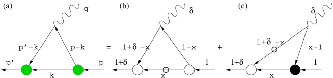
Figure 1: The covariant triangle diagram (a) is represented as the sum of a LF valence diagram (b) defined in the region $0<k^{+}<p^{+}$ and the nonvalence diagram (b) defined in $p^{+}<k^{+}<p^{\prime+}$. $\delta=q^{+}/p^{+}=p^{\prime+}/p^{+}-1$. The white and black blobs at the boson-fermion vertices in (b) and (c) represent the LF wave-function and non-wave-function vertices, respectively, for a bound-state boson. In the SM, however, $W^{\pm}$ gauge bosons are point particles and those blobs reduce to point vertices. The small circles in (b) and (c) represent the (on-shell) mass pole of the fermion propagator determined from the $k^{-}$-integration.

III.1 Details of the Computation

We first determine the trace in the covariant expression. It is

$$T^{\mu}_{h^{\prime}h} = {\rm Tr}[\not\!\epsilon^{*}_{h^{\prime}}(1-\gamma_{5})(\not\!k+m_{2})\not\!\epsilon_{h}(1-\gamma_{5})(\not\!k-\not\!p+m_{1})\gamma^{\mu}(\not\!k-\not\!p^{\prime}+m_{1})]$$ (22)

$$= 2(T^{\mu}_{h^{\prime}h})_{CP^{+}}+2(T^{\mu}_{h^{\prime}h})_{CP^{-}}$$

$$= \;2{\rm Tr}[\not\!\epsilon^{*}_{h^{\prime}}\not\!k\not\!\epsilon_{h}(\not\!k-\not\!p+m_{1})\gamma^{\mu}(\not\!k-\not\!p^{\prime}+m_{1})],$$

$$+2{\rm Tr}[\gamma_{5}\not\!\epsilon^{*}_{h^{\prime}}\not\!k\not\!\epsilon_{h}(\not\!k-\not\!p+m_{1})\gamma^{\mu}(\not\!k-\not\!p^{\prime}+m_{1})].$$

The two traces determine two parts of the triangle diagram: a $CP$-even one and a $CP$-odd one. We shall not pursue the latter here. The $CP$-even part is found to be

$$(T^{\mu}_{h^{\prime}h})_{CP^{+}} = 4\left\{\,k^{\mu}\left[4\,\epsilon^{*}_{h^{\prime}}\cdot k\,\epsilon_{h}\cdot k-\epsilon^{*}_{h^{\prime}}\cdot p\,\epsilon_{h}\cdot p^{\prime}-\epsilon^{*}_{h^{\prime}}\cdot\epsilon_{h}\,(k^{2}-p\cdot p^{\prime}+m^{2}_{1})\right]\right.$$

$$\left.+\,p^{\mu}\left[-2\epsilon^{*}_{h^{\prime}}\cdot k\,\epsilon_{h}\cdot k+\epsilon^{*}_{h^{\prime}}\cdot k\,\epsilon_{h}\cdot p^{\prime}+\epsilon^{*}_{h^{\prime}}\cdot\epsilon_{h}\,(k^{2}-k\cdot p^{\prime})\right]\right.$$

$$\left.+\,p^{\prime\mu}\left[-2\epsilon^{*}_{h^{\prime}}\cdot k\,\epsilon_{h}\cdot k+\epsilon^{*}_{h^{\prime}}\cdot p\,\epsilon_{h}\cdot k+\epsilon^{*}_{h^{\prime}}\cdot\epsilon_{h}\,(k^{2}-k\cdot p)\right]\right.$$

$$\left.-\,\epsilon^{\mu}_{h}\left[\epsilon^{*}_{h^{\prime}}\cdot k\,(k^{2}-2k\cdot p+p^{\prime}\cdot p-m^{2}_{1})+\epsilon^{*}_{h^{\prime}}\cdot p\,(k^{2}-k\cdot p^{\prime})\right]\right.$$

$$\left.-\,\epsilon^{*\mu}_{h^{\prime}}\left[\epsilon_{h}\cdot k\,(k^{2}-2k\cdot p^{\prime}+p^{\prime}\cdot p-m^{2}_{1})+\epsilon\cdot p^{\prime}\,(k^{2}-k\cdot p)\right]\right\}.$$

We use the Feynman parametrization for the three propagators, e.g.,

$$\frac{1}{D_{k}D_{0}D^{\prime}_{0}} = 2\int^{1}_{0}dx\int^{1-x}_{0}dy\frac{1}{[xD_{0}+yD^{\prime}_{0}+(1-x-y)D_{k}]^{3}}.$$ (24)

We shall compute the integrals over the momentum by shifting the integration variable from $k$ to $k^{\prime}=k-(xp+yp^{\prime})$, although we are aware of the fact that a shift is not permitted unless the integral can be shown to diverge at most logarithmically. We shall return to this point later. Then one finds a denominator that is an even function of $k^{\prime}$:

$$D=[k-(xp+yp^{\prime})]^{2}+(x+y)(1-x-y)M^{2}_{W}-(x+y)m^{2}_{1}-(1-x-y)m^{2}_{2}+xyq^{2}.$$ (25)

We thus can write the denominator function in the form

$$D=k^{\prime 2}-M^{2}_{W}C^{2}_{\rm cov}.$$ (26)

Using the notation given in Eq. (14), the mass function is

$$-C^{2}_{\rm cov}=(x+y)(1-x-y)-(x+y)\Delta-(1-x-y){\cal E}-4xy\eta.$$ (27)

The shift in momentum variable must be applied to the trace too. Doing so and discarding the terms odd in $k^{\prime}$ gives the new numerator given by

$$S^{\mu}_{h^{\prime}h}:=(T^{\mu}_{h^{\prime}h})_{CP^{+}} = 4\left\{\,\epsilon^{*}_{h^{\prime}}\cdot\epsilon_{h}\,\left[p^{\mu}\left(\frac{1-x}{2}k^{\prime 2}+\{(1-x)(x+y)^{2}-y\}M^{2}_{W}-(1-x)xyq^{2}-xm_{1}^{2}\right)\right.\right.$$ (28)

$$\left.\left.\quad\quad\quad+p^{\prime\mu}\left(\frac{1-y}{2}k^{\prime 2}+\{(1-y)(x+y)^{2}-x\}M^{2}_{W}-(1-y)xyq^{2}-ym_{1}^{2}\right)\right]\right.$$

$$\left.+\epsilon^{*}_{h^{\prime}}\cdot p\,\epsilon_{h}^{\mu}\left[-\frac{1+x}{2}k^{\prime 2}-(x+y-1)(x^{2}+(1+x)y)M^{2}_{W}+x^{2}yq^{2}+xm^{2}_{1}\right]\right.$$

$$\left.+\epsilon_{h}\cdot p^{\prime}\,\epsilon_{h^{\prime}}^{*\mu}\left[-\frac{1+y}{2}k^{\prime 2}-(x+y-1)(y^{2}+(1+y)x)M^{2}_{W}+xy^{2}q^{2}+ym^{2}_{1}\right]\right.$$

$$\left.+\epsilon^{*}_{h^{\prime}}\cdot p\;\epsilon_{h}\cdot p^{\prime}\;(2xy)\left[(2x-1)p^{\mu}+(2y-1)p^{\prime\mu}\right]\rule{0.0pt}{12.91663pt}\right\}.$$

From Eq. (25), we see that part of the denominator is symmetric under interchange of $p$ and $p^{\prime}$ and $x$ and $y$. It is not difficult to show that only the numerator symmetric in $x$ and $y$ can survive the integration. Therefore, we may symmetrize the formal expression (28). We find for the symmetrized trace

$$(S^{\mu}_{h^{\prime}h})_{\rm symm}=\epsilon^{*}_{h^{\prime}}\cdot\epsilon_{h}\,(p+p^{\prime})^{\mu}f_{1}+(\epsilon^{*}_{h^{\prime}}\cdot p\,\epsilon_{h}^{\mu}+\epsilon_{h}\cdot p^{\prime}\,\epsilon_{h^{\prime}}^{*\mu})f_{2}+\epsilon^{*}_{h^{\prime}}\cdot p\;\epsilon_{h}\cdot p^{\prime}(p+p^{\prime})^{\mu}f_{3},$$ (29)

where the functions $f_{1}$, $f_{2}$, and $f_{3}$ are

$$f_{1}=f^{1}_{1}k^{\prime 2}+f^{0}_{1} = (2-x-y)\;k^{\prime 2}$$

$$-2[(x+y)(1-x-y)^{2}M^{2}_{W}+(2-x-y)xyq^{2}+(x+y)m^{2}_{1}],$$

$$f_{2}=f^{1}_{2}k^{\prime 2}+f^{0}_{2} = -(2+x+y)k^{\prime 2}$$

$$+2(x+y)[(1-(x+y)^{2})M^{2}_{W}+xyq^{2}+m^{2}_{1}],$$

$$f_{3} = 8xy(x+y-1).$$ (30)

Comparing Eq. (30) with Eq. (15), we can read off the integrands for the three form factors. In the manifestly covariant calculation, we first obtain the form factors $F_{i}(i=1,2,3)$ using dimensional regularization DR₄:

$$F_{1}(Q^{2}) = \frac{g^{2}Q_{f}}{4\pi^{2}}\int^{1}_{0}dx\int^{1-x}_{0}dy\biggl{\{}-(2-x-y)\left[\frac{1}{\epsilon}-\gamma-\frac{1}{2}+\ln\frac{4\pi\mu^{2}}{M^{2}_{W}C^{2}_{\rm cov}}\right]+\frac{1}{2}\frac{f^{0}_{1}}{M^{2}_{W}C^{2}_{\rm cov}}\biggr{\}}$$

$$F_{2}(Q^{2}) = \frac{g^{2}Q_{f}}{4\pi^{2}}\int^{1}_{0}dx\int^{1-x}_{0}dy\biggl{\{}(2+x+y)\left[\frac{1}{\epsilon}-\gamma-\frac{1}{2}+\ln\frac{4\pi\mu^{2}}{M^{2}_{W}C^{2}_{\rm cov}}\right]+\frac{1}{2}\frac{f^{0}_{2}}{M^{2}_{W}C^{2}_{\rm cov}}\biggr{\}}$$

$$F_{3}(Q^{2}) = \frac{g^{2}Q_{f}}{4\pi^{2}}\int^{1}_{0}dx\int^{1-x}_{0}dy\;\frac{8xy(x+y-1)}{C^{2}_{\rm cov}},$$ (31)

where $\epsilon$ is defined in the Appendix.

In order to obtain the form factors using PVR or SMR, one introduces fictitious particles with mass $\Lambda$. In true Pauli-Villars regularization one replaces the amplitude $M^{\mu}(m_{1},m_{2})$ by the amplitude $M^{\rm Reg}=M^{\mu}(m_{1},m_{2})-M^{\mu}(\Lambda_{1},m_{2})$ or $M^{\rm Reg}=M^{\mu}(m_{1},m_{2})-M^{\mu}(m_{1},\Lambda_{2})$, depending on whether one chooses to replace the propagator of the struck fermion or the spectator fermion, respectively, by the combination $(\not\!p-m)^{-1}-(\not\!p-\Lambda)^{-1}$. The SMR procedure BCJ01 consists in replacing the $\gamma f\bar{f}$-vertex $\gamma^{\mu}$ by the vertex $S_{\Lambda}(p^{\prime})\gamma^{\mu}S_{\Lambda}(p)$ using the SMR function $S_{\Lambda}(p)=\Lambda^{2}/(p^{2}-\Lambda^{2}+i\varepsilon)$. For the purpose of making the situation transparent, we define the function

$$-C^{2}(m_{a},m_{b})=(x+y)(1-x-y)M^{2}_{W}-xm^{2}_{a}-ym^{2}_{b}-(1-x-y)m^{2}_{2}+xy\;q^{2},$$ (32)

where $C^{2}(m_{1},m_{1})=M^{2}_{W}C^{2}_{\rm cov}$. The full result using SMR for the form factors of a vector meson (or spin-1 bound-states) can be found in Ref. BCJ02 . The SMR result amounts to the following replacements of the logarithmic term and the factor $1/C^{2}_{\rm cov}$ in the nonlogarithmic parts in Eq. (31):

$$\ln(C^{2}_{\rm cov}) \to \ln\left(\frac{C^{2}(m_{1},m_{1})C^{2}(\Lambda,\Lambda)}{C^{2}(m_{1},\Lambda)C^{2}(\Lambda,m_{1})}\right),$$

$$\frac{1}{M^{2}_{W}C^{2}_{\rm cov}} \to \frac{1}{C^{2}(m_{1},m_{1})}-\frac{1}{C^{2}(m_{1},\Lambda)}-\frac{1}{C^{2}(\Lambda,m_{1})}+\frac{1}{C^{2}(\Lambda,\Lambda)}.$$ (33)

Note that the substitution of $\Lambda$ for $m_{1}$ only affects the denominators. In the case of PVR, the propagator mass is replaced, affecting both the numerator and the denominator. The result is given by the substitutions in the integrands ${\cal F}_{i}$ defining the form factors $F_{i}$

$${\cal F}_{i}(m_{1},m_{2})\to{\cal F}_{i}(m_{1},m_{2})-{\cal F}_{i}(\Lambda_{1},m_{2}),\quad(i=1,2,3)$$ (34)

for Pauli-Villars in the fermion line connected to the photon and

$${\cal F}_{i}(m_{1},m_{2})\to{\cal F}_{i}(m_{1},m_{2})-{\cal F}_{i}(m_{1},\Lambda_{2}),\quad(i=1,2,3)$$ (35)

for the regularization involving the spectator only. The infinities that plague $F_{1}$ and $F_{2}$, represented by the terms in Eq. (31) containing the factor $1/\epsilon$ are also found in SMR or PVR if the limit $\Lambda\to\infty$ is taken. In particular, we find for the SMR case

$$-\ln\left(\frac{C^{2}(m_{1},\Lambda)C^{2}(\Lambda,m_{1})}{C^{2}(m_{1},m_{1})C^{2}(\Lambda,\Lambda)}\right)\to-\ln\left(\frac{\Lambda^{2}}{M^{2}_{W}}\right)+\ln\left(\frac{x+y}{xy}\right)+\ln(C^{2}_{\rm cov}),$$ (36)

while the nonlogarithmic terms containing $\Lambda$ vanish.

For the two PVR cases, $m_{1}\to\Lambda_{1}$ (PV₁) and $m_{2}\to\Lambda_{2}$ (PV₂), we find the logarithm to be replaced by

$$\ln(C^{2}_{\rm cov}) \to -\ln\left(\frac{\Lambda^{2}_{1}}{M^{2}_{W}}\right)-\ln(x+y)+\ln(C^{2}_{\rm cov}),$$

$$\ln(C^{2}_{\rm cov}) \to -\ln\left(\frac{\Lambda^{2}_{2}}{M^{2}_{W}}\right)-\ln(1-x-y)+\ln(C^{2}_{\rm cov}),$$ (37)

respectively. The nonlogarithmic term in the integrand of $F_{1}$($F_{2}$) gets corrected by $-1$($+1$) for PV₁. For PV₂, the corrections to the nonlogarithmic terms are zero in the limit $\Lambda_{2}\to\infty$ because $m_{2}$ does not occur in the numerators.

Clearly, the infinity in the DR case is recovered as a term $\ln\Lambda$ in SMR or PVR. There appear, however, finite terms that contribute to the finite parts of the form factors $F_{1}$ and $F_{2}$. These terms are independent of the masses of the fermions and, when integrated over $x$ and $y$, appear as pure numbers.

III.2 Summary of Covariant Results

DR₄
The three form factors obtained in DR₄ can be summarized as

$$F_{1}(Q^{2}) = \frac{g^{2}Q_{f}}{4\pi^{2}}\biggl{\{}-\frac{2}{3}\left(\frac{1}{\epsilon}-\gamma-\frac{1}{2}\right)+\int^{1}_{0}dx\int^{1-x}_{0}dy\left[-(2-x-y)\ln\frac{4\pi\mu^{2}}{M^{2}_{W}C^{2}_{\rm cov}}+\frac{1}{2}\frac{f^{0}_{1}}{M^{2}_{W}C^{2}_{\rm cov}}\right]\biggr{\}}$$

$$F_{2}(Q^{2}) = \frac{g^{2}Q_{f}}{4\pi^{2}}\biggl{\{}\frac{4}{3}\left(\frac{1}{\epsilon}-\gamma-\frac{1}{2}\right)+\int^{1}_{0}dx\int^{1-x}_{0}dy\left[(2+x+y)\ln\frac{4\pi\mu^{2}}{M^{2}_{W}C^{2}_{\rm cov}}+\frac{1}{2}\frac{f^{0}_{2}}{M^{2}_{W}C^{2}_{\rm cov}}\right]\biggr{\}}$$

$$F_{3}(Q^{2}) = \frac{g^{2}Q_{f}}{4\pi^{2}}\int^{1}_{0}dx\int^{1-x}_{0}dy\;\frac{8xy(x+y-1)}{C^{2}_{\rm cov}}.$$ (38)

The physical quantity, -$\Delta\kappa$, corresponds to

$$2F_{1}(Q^{2})+F_{2}(Q^{2}) = \frac{g^{2}Q_{f}}{4\pi^{2}}\int^{1}_{0}dx\int^{1-x}_{0}dy\left[-(2-3x-3y)\ln\frac{4\pi\mu^{2}}{M^{2}_{W}C^{2}_{\rm cov}}+\frac{1}{2}\frac{2f^{0}_{1}+f^{0}_{2}}{M^{2}_{W}C^{2}_{\rm cov}}\right]$$ (39)

$$= \frac{g^{2}Q_{f}}{4\pi^{2}}\int^{1}_{0}dx\int^{1-x}_{0}dy\left[(2-3x-3y)\ln C^{2}_{\rm cov}+\frac{1}{2}\frac{2f^{0}_{1}+f^{0}_{2}}{M^{2}_{W}C^{2}_{\rm cov}}\right].$$

The singular part of $2F_{1}(Q^{2})+F_{2}(Q^{2})$ is cancelled out and the dependence on the mass scale $\mu$ also vanishes when integrated over $x$ and $y$. Changing the variables $x$ and $y$ to $t=x+y$ and $u=x-y$, the relevant integral becomes

$$\frac{1}{2}\int^{1}_{0}dt\int^{t}_{-t}du(2-3t)\ln\frac{4\pi\mu^{2}}{M^{2}_{W}}=\int^{1}_{0}dt\;t(2-3t)\ln\frac{4\pi\mu^{2}}{M^{2}_{W}}$$ (40)

which vanishes for any mass scale $\mu$. This indicates that $2F_{1}+F_{2}$ is defined by a conditionally convergent integral. At $q^{2}=0$, the part containing $\ln(C^{2}_{\rm cov})$ can be cast in the form of a combination of integrals $I_{n}$ by performing an integration by parts;

$$F_{2}(0)+2F_{1}(0) = -\frac{g^{2}Q_{f}}{4\pi^{2}}\int^{1}_{0}dt\left\{(3t^{2}-2t)\ln(t^{2}-tF+{\cal E})+\frac{3t^{4}-4t^{3}+t^{2}(1+\Delta)}{t^{2}-tF+{\cal E}}\right\}$$ (41)

$$= -\frac{g^{2}Q_{f}}{4\pi^{2}}\int^{1}_{0}dt\frac{t^{4}-(F-2)t^{3}+(2\Delta-{\cal E})t^{2}}{t^{2}-tF+{\cal E}}.$$

In this way, we recover the well known results for the physical quantities  CN87

$$F_{2}(0)+2F_{1}(0) = -\frac{g^{2}Q_{f}}{4\pi^{2}}[I_{4}-(F-2)I_{3}+(2\Delta-{\cal E})I_{2}],$$

$$F_{3}(0) = -\frac{g^{2}Q_{f}}{4\pi^{2}}\;\frac{4}{3}[I_{3}-I_{4}].$$ (42)

Since the form factor $F_{3}$ needs no regularization, we do not include it in the summary below, where we give the results for the other regularizations.

SMR

$$F_{1}(Q^{2}) = \frac{g^{2}Q_{f}}{4\pi^{2}}\biggl{\{}-\frac{2}{3}\ln\frac{\Lambda^{2}}{M^{2}_{W}}+\frac{31}{18}+\int^{1}_{0}dx\int^{1-x}_{0}dy\left[-(2-x-y)\ln\frac{1}{C^{2}_{\rm cov}}+\frac{1}{2}\frac{f^{0}_{1}}{M^{2}_{W}C^{2}_{\rm cov}}\right]\biggr{\}}$$

$$F_{2}(Q^{2}) = \frac{g^{2}Q_{f}}{4\pi^{2}}\biggl{\{}\frac{4}{3}\ln\frac{\Lambda^{2}}{M^{2}_{W}}-\frac{59}{18}+\int^{1}_{0}dx\int^{1-x}_{0}dy\left[(2+x+y)\ln\frac{1}{C^{2}_{\rm cov}}+\frac{1}{2}\frac{f^{0}_{2}}{M^{2}_{W}C^{2}_{\rm cov}}\right]\biggr{\}}$$

$$2F_{1}(Q^{2})+F_{2}(Q^{2}) = \frac{g^{2}Q_{f}}{4\pi^{2}}\biggl{\{}\frac{1}{6}+\int^{1}_{0}dx\int^{1-x}_{0}dy\left[(2-3x-3y)\ln C^{2}_{\rm cov}+\frac{1}{2}\frac{2f^{0}_{1}+f^{0}_{2}}{M^{2}_{W}C^{2}_{\rm cov}}\right]\biggr{\}},$$ (43)

PV₁

$$F_{1}(Q^{2}) = \frac{g^{2}Q_{f}}{4\pi^{2}}\biggl{\{}-\frac{2}{3}\ln\frac{\Lambda^{2}}{M^{2}_{W}}+\frac{8}{9}+\int^{1}_{0}dx\int^{1-x}_{0}dy\left[-(2-x-y)\ln\frac{1}{C^{2}_{\rm cov}}+\frac{1}{2}\frac{f^{0}_{1}}{M^{2}_{W}C^{2}_{\rm cov}}\right]\biggr{\}}$$

$$F_{2}(Q^{2}) = \frac{g^{2}Q_{f}}{4\pi^{2}}\biggl{\{}\frac{4}{3}\ln\frac{\Lambda^{2}}{M^{2}_{W}}-\frac{10}{9}+\int^{1}_{0}dx\int^{1-x}_{0}dy\left[(2+x+y)\ln\frac{1}{C^{2}_{\rm cov}}+\frac{1}{2}\frac{f^{0}_{2}}{M^{2}_{W}C^{2}_{\rm cov}}\right]\biggr{\}}$$

$$2F_{1}(Q^{2})+F_{2}(Q^{2}) = \frac{g^{2}Q_{f}}{4\pi^{2}}\biggl{\{}\frac{2}{3}+\int^{1}_{0}dx\int^{1-x}_{0}dy\left[(2-3x-3y)\ln C^{2}_{\rm cov}+\frac{1}{2}\frac{2f^{0}_{1}+f^{0}_{2}}{M^{2}_{W}C^{2}_{\rm cov}}\right]\biggr{\}},$$ (44)

PV₂

$$F_{1}(Q^{2}) = \frac{g^{2}Q_{f}}{4\pi^{2}}\biggl{\{}-\frac{2}{3}\ln\frac{\Lambda^{2}}{M^{2}_{W}}+\frac{8}{9}+\int^{1}_{0}dx\int^{1-x}_{0}dy\left[-(2-x-y)\ln\frac{1}{C^{2}_{\rm cov}}+\frac{1}{2}\frac{f^{0}_{1}}{M^{2}_{W}C^{2}_{\rm cov}}\right]\biggr{\}}$$

$$F_{2}(Q^{2}) = \frac{g^{2}Q_{f}}{4\pi^{2}}\biggl{\{}\frac{4}{3}\ln\frac{\Lambda^{2}}{M^{2}_{W}}-\frac{19}{9}+\int^{1}_{0}dx\int^{1-x}_{0}dy\left[(2+x+y)\ln\frac{1}{C^{2}_{\rm cov}}+\frac{1}{2}\frac{f^{0}_{2}}{M^{2}_{W}C^{2}_{\rm cov}}\right]\biggr{\}}$$

$$2F_{1}(Q^{2})+F_{2}(Q^{2}) = \frac{g^{2}Q_{f}}{4\pi^{2}}\biggl{\{}-\frac{1}{3}+\int^{1}_{0}dx\int^{1-x}_{0}dy\left[(2-3x-3y)\ln C^{2}_{\rm cov}+\frac{1}{2}\frac{2f^{0}_{1}+f^{0}_{2}}{M^{2}_{W}C^{2}_{\rm cov}}\right]\biggr{\}}.$$ (45)

IV Light-front calculation

The covariant amplitude shown in Fig. 1(a) is in general believed to be equivalent to the sum of the LF valence diagram (b) and the nonvalence diagram (c), where the notation $\delta=q^{+}/p^{+}=p^{\prime+}/p^{+}-1$ is used. For amplitudes that are defined by convergent integrals this belief is well founded NEL ; SCH . However, for amplitudes that require regularization the situation is not straightforward and a caution is necessary. In particular, the LFD dispersion relation between the energy and the momenta upsets the usual power counting in theories involving spin. We give the general formalism first and subsequently give the results of the detailed calculations.

IV.1 General Formalism

In the LF calculation, integrating over $k^{-}$ leads to the time-ordered diagrams shown in Fig. 1(b) and (c). The pole value $k^{-}=k^{-}_{\rm pole}$ is obtained from the on-mass-shell condition for the corresponding fermion denoted by small circles in the diagrams (b) and (c). The diagram (b) is called the valence part. Depending on the helicity combination there may be a second contribution, that for $q^{+}>0$ would be the diagram (c) called the nonvalence part, but in our kinematics reduces to the zero-mode contribution which is the limit $\delta\to 0$ of the nonvalence part. One can directly calculate the trace term by substitution of $k^{-}_{\rm pole}$ in $S^{\mu}_{h^{\prime}h}$.

The zero-mode contribution is found using the following identity

$$\not\!p+m_{f}=(\not\!{p_{\rm on}}+m_{f})+\frac{1}{2}\gamma^{+}(p^{-}-p^{-}_{\rm on}),$$ (46)

where the subscript (on) denotes the on-mass-shell ($p^{2}=m^{2}_{f}$) fermion momentum, i.e., $p^{-}=p^{-}_{\rm on}=(m^{2}_{f}+\vec{p}^{\,2}_{\perp})/p^{+}$. Then the trace term $T^{+}_{h^{\prime}h}$ of the fermion propagators in Eq. (21) is given by

$$(T^{+}_{h^{\prime}h})_{CP^{+}}=(T^{+}_{h^{\prime}h})_{\rm val}+(T^{+}_{h^{\prime}h})_{\rm zm},$$ (47)

where $(T^{+}_{h^{\prime}h})_{\rm val}$ is obtained by substitution of $k^{-}=\frac{\vec{k}^{\,2}_{\perp}+m^{2}_{2}}{xp^{+}}$ in Eq. (LABEL:eq.III.030) and $(T^{+}_{h^{\prime}h})_{\rm zm}$ is given by

$$(T^{+}_{h^{\prime}h})_{\rm zm} = \frac{1}{2}(k^{-}-k^{-}_{\rm on}){\rm Tr}[\not\!\epsilon^{*}_{h^{\prime}}\gamma^{+}\not\!\epsilon_{h}(\not\!k-\not\!p+m_{1})\gamma^{+}(\not\!k-\not\!p^{\prime}+m_{1})],$$ (48)

where $k^{-}=p^{\prime-}+\frac{m^{2}_{1}+(\vec{k}_{\perp}-\vec{p^{\prime}}_{\perp})^{2}}{k^{+}-p^{\prime+}}$. As we shall show below, the LF valence contribution comes exclusively from the on-mass-shell propagating part, and the zero-mode (if it exists) from the instantaneous part given by Eq. (48).

Using the reference frame (See Eq. (17)) with the LF gauge, we obtain for the trace terms $(T^{+}_{h^{\prime}h})_{\rm val}$ and $(T^{+}_{h^{\prime}h})_{\rm zm}$ the expressions:

$$(T^{+}_{++})_{\rm val} = \frac{4p^{+}}{x}\biggl{[}x^{2}m^{2}_{1}+(1-x)^{2}m^{2}_{2}+(2x^{2}-2x+1)\left(\vec{k}^{2}_{\perp}-ixQk_{y}-\frac{x^{2}}{4}Q^{2}\right)\biggr{]},$$

$$(T^{+}_{+0})_{\rm val} = \frac{\sqrt{2}p^{+}}{xM_{W}}\left\{(2k_{x}-2ik_{y}-Qx)(2x-1)\left[(k_{x}+Qx/2)^{2}+k^{2}_{y}+x(1-x)M^{2}_{W}\right]\right.$$

$$\left.\quad\quad\quad+(2k_{x}-2ik_{y}+Qx)\left[xm^{2}_{1}-(1-x)m^{2}_{2}\right]\right\},$$

$$(T^{+}_{+-})_{\rm val} = 8(1-x)p^{+}\left\{(k_{x}-ik_{y})^{2}-Q^{2}x^{2}/4\right\},$$

$$(T^{+}_{00})_{\rm val} = \frac{4p^{+}}{xM^{2}_{W}}\left\{(k^{2}_{x}+k^{2}_{y}-Q^{2}x^{2}/4)(m^{2}_{1}+m^{2}_{2})+m^{2}_{1}m^{2}_{2}+\right.$$

$$\left.\left[(k_{x}+Qx/2)^{2}+k^{2}_{y}+x(1-x)M^{2}_{W}\right]\left[(k_{x}-Qx/2)^{2}+k^{2}_{y}+x(1-x)M^{2}_{W}\right]\right\},$$

and

$$(T^{+}_{++})_{\rm zm} = 4(p^{+})^{2}(k^{-}-k^{-}_{\rm on})(1-x)^{2},$$

$$(T^{+}_{+-})_{\rm zm} = 0,$$

$$(T^{+}_{+0})_{\rm zm} = \frac{4(p^{+})^{2}}{\sqrt{2}M_{W}}(k^{-}-k^{-}_{\rm on})(1-x)[-k_{x}+ik_{y}-Qx/2],$$

$$(T^{+}_{00})_{\rm zm} = \frac{4(p^{+})^{2}}{M^{2}_{W}}(k^{-}-k^{-}_{\rm on})[\vec{k}^{\,2}_{\perp}-Q^{2}x^{2}/4+m^{2}_{1}],$$ (50)

where $x=k^{+}/p^{+}$ and $k^{-}_{\rm\rm on}=\frac{\vec{k}^{\,2}_{\perp}+m^{2}_{2}}{xp^{+}}$. Since $(k^{-}-k^{-}_{\rm on})$ is factored out in $(T^{+}_{h^{\prime}h})_{\rm zm}$, we shall denote the rest by $R^{+}_{h^{\prime}h}$,i.e., $(T^{+}_{h^{\prime}h})_{\rm zm}=(k^{-}-k^{-}_{\rm on})R^{+}_{h^{\prime}h}$.

IV.1.1 Valence contribution

The valence contribution to the current matrix elements is given by

$$(G^{+}_{h^{\prime}h})_{\rm val} = \frac{-g^{2}Q_{f}}{(2\pi)^{3}}\int^{1}_{0}\frac{dx}{x(1-x)^{2}}\int d^{2}k_{\perp}\left(T^{+}_{h^{\prime}h}\right)_{\rm val}$$ (51)

$$\times\frac{1}{M^{2}_{W}+Q^{2}/4-(\vec{k}^{\,2}_{\perp}+m^{2}_{2})/x-((\vec{k}_{\perp}-\vec{p}_{\perp})^{2}+m^{2}_{1})/(1-x)}$$

$$\times\frac{1}{M^{2}_{W}+Q^{2}/4-(\vec{k}^{\,2}_{\perp}+m^{2}_{2})/x-((\vec{k}_{\perp}-\vec{p}^{\prime}_{\perp})^{2}+m^{2}_{1})/(1-x)}.$$

Here, we aim at performing the integral over $\vec{k}_{\perp}$ analytically, so we proceed as in the covariant case by introducing a Feynman parameter to obtain in an obvious notation

$$\frac{1}{D_{1}D_{2}}=\int^{1}_{0}\frac{dy}{[yD_{1}+(1-y)D_{2}]^{2}},$$ (52)

where

$$D = yD_{1}+(1-y)D_{2}$$

$$= M^{2}_{W}+Q^{2}/4-\frac{\vec{k}^{\,2}_{\perp}+m^{2}_{2}}{x}-\frac{\vec{k}^{\,2}_{\perp}+Q^{2}/4+m^{2}_{1}}{1-x}+(1-2y)\frac{k_{x}Q}{1-x}.$$

By completing the square in $k_{x}$ and performing the following shift in the integration variables

$$k^{\prime}_{x}=k_{x}-\frac{1-2y}{2}Qx,\quad k^{\prime}_{y}=k_{y},$$ (54)

one obtains a denominator that is symmetric in $k^{\prime}_{x}$ and $k^{\prime}_{y}$:

$$D=M^{2}_{W}+Q^{2}/4-\frac{1}{x(1-x)}\{\vec{k}^{\,\prime 2}_{\perp}+xm^{2}_{1}+(1-x)m^{2}_{2}+x(1-x(1-2y)^{2}Q^{2}/4)\}.$$ (55)

After performing the same shift in the trace, one can neglect the terms that are odd in the components of $\vec{k}^{\,\prime}_{\perp}$ as their contributions vanish because of symmetry. We denote the shifted trace by $S^{+}_{h^{\prime}h}(\vec{k}^{\,\prime}_{\perp})_{\rm val}$.

The final result can now be written in a succinct form

$$(G^{+}_{h^{\prime}h})_{\rm val} = \frac{-g^{2}Q_{f}}{(2\pi)^{3}}\int^{1}_{0}dxx\,\int^{1}_{0}dy\,\int d^{2}k_{\perp}\frac{S^{+}_{h^{\prime}h}(\vec{k}_{\perp})_{\rm val}}{(\vec{k}^{2}_{\perp}+M^{2}_{W}D_{\rm LF})^{2}},$$ (56)

where the integration variable $\vec{k}^{\,\prime}_{\perp}$ is changed to $\vec{k}_{\perp}$. The function $D_{\rm LF}$ is

$$D_{\rm LF}=x\Delta+(1-x){\cal E}-x(1-x)+4x^{2}y(1-y)\eta.$$ (57)

Before writing down the traces for the different helicity combinations, we do the zero-mode first and show that their contributions, if any remain, can be written in a form similar to the valence part.

IV.1.2 Zero-mode contribution

The zero-mode is the contribution from the nonvalence part in the limit $q^{+}\to 0$ BCJ02 . In our kinematics, it is equal to the limit $\delta\to 0$ of

$$(G^{+}_{h^{\prime}h})_{\rm zm} = \frac{-g^{2}Q_{f}}{(2\pi)^{3}p^{+}}\int^{1+\delta}_{1}\frac{dx}{x(x-1)(x-1-\delta)}\,\int d^{2}k_{\perp}$$ (58)

$$\times\frac{R^{+}_{h^{\prime}h}}{\frac{\delta(M^{2}_{W}+Q^{2}/4)}{1+\delta}+\frac{(\vec{k}_{\perp}-\vec{p}^{\,\prime}_{\perp})^{2}+m^{2}_{1}}{1+\delta-x}+\frac{(\vec{k}_{\perp}-\vec{p}_{\perp})^{2}+m^{2}_{1}}{x-1}},$$

where the factor $(k^{-}-k^{-}_{\rm on})$ in the trace term $(T^{+}_{h^{\prime}h})_{\rm zm}=(k^{-}-k^{-}_{\rm on})R^{+}_{h^{\prime}h}$ has been cancelled out by the same factor in one of the LF energy denominators. With the substitutions

$$x=1+\delta z,\quad k_{x}=k^{\prime}_{x}-\frac{1-x+\delta/2}{\delta}=k^{\prime}_{x}-\frac{1-2z}{2}Q,\quad k_{y}=k^{\prime}_{y},$$ (59)

and taking the limit we obtain

$$(G^{+}_{h^{\prime}h})_{\rm zm}=\frac{g^{2}Q_{f}}{(2\pi)^{3}p^{+}}\int^{1}_{0}dz\,\int d^{2}k^{\prime}_{\perp}\frac{R^{+}_{h^{\prime}h}(\vec{k}^{\,\prime}_{\perp})}{\vec{k}^{\,\prime 2}_{\perp}+m^{2}_{1}+z(1-z)Q^{2}}.$$ (60)

Note here that $(G^{+}_{h^{\prime}h})_{\rm zm}$ vanishes if $R^{+}_{h^{\prime}h}$(or $(T^{+}_{h^{\prime}h})_{\rm zm}$) carries the factor $(1-x)^{n}(n\geq 1)$ because $1-x=-\delta z$ goes to zero as $\delta\rightarrow 0$. This is the case for $(T^{+}_{++})_{\rm zm}$ and $(T^{+}_{+0})_{\rm zm}$ as shown in Eq. (50). Thus, the nonvanishing zero-mode contribution can occur only in $(G^{+}_{00})_{\rm zm}$. A straightforward analysis shows that $G^{+}_{00}$ has indeed a zero-mode. The shifted trace in the limit $\delta\rightarrow 0$ yields

$$R^{+}_{00}(\vec{k}^{\,\prime}_{\perp})=\frac{4(p^{+})^{2}}{M^{2}_{W}}[\vec{k}^{\,\prime 2}_{\perp}+m^{2}_{1}-z(1-z)Q^{2}].$$ (61)

Consequently, changing the integration variables $z$ and $\vec{k}^{\prime}_{\perp}$ to $x$ and $\vec{k}_{\perp}$, we find for the zero-mode contribution to $G^{+}_{00}$:

$$(G^{+}_{00})_{\rm zm}=\frac{4g^{2}Q_{f}p^{+}}{(2\pi)^{3}}\int^{1}_{0}dx\,\int d^{2}k_{\perp}\frac{\vec{k}^{2}_{\perp}+m^{2}_{1}-x(1-x)Q^{2}}{\vec{k}^{2}_{\perp}+m^{2}_{1}+x(1-x)Q^{2}}.$$ (62)

IV.2 Individual Current Matrix Elements

Here we give the detailed results of individual current matrix elements.

IV.2.1 $G^{+}_{++}$

From the procedure illustrated in the previous subsection IV.1, we find

$$\left(S^{+}_{++}(\vec{k}_{\perp})\right)_{\rm val}=\frac{4p^{+}}{x}\left(N^{1}_{++}\vec{k}^{2}_{\perp}+M^{2}_{W}N^{0}_{++}\right),$$ (63)

where the numerator functions are given by

$$M^{2}_{W}N^{0}_{++} = m^{2}_{1}x^{2}+m^{2}_{2}(1-x)^{2}-(2x^{2}-2x+1)y(1-y)x^{2}Q^{2},$$

$$N^{1}_{++} = 2x^{2}-2x+1.$$ (64)

Thus, we get

$$(G^{+}_{++})_{\rm val} = -\frac{4g^{2}Q_{f}p^{+}}{(2\pi)^{3}}\int^{1}_{0}dx\;\int^{1}_{0}dy\;\int d^{2}k_{\perp}\;\frac{\vec{k}^{\,2}_{\perp}N^{1}_{++}+M^{2}_{W}N^{0}_{++}}{[\vec{k}^{\,2}_{\perp}+M^{2}_{W}D_{\rm LF}]^{2}}.$$ (65)

As explained in subsection IV.1, $(G^{+}_{++})_{\rm zm}$ vanishes.

IV.2.2 $G^{+}_{+0}$

Following the same procedure, we find

$$\left(S^{+}_{+0}(\vec{k}_{\perp})\right)_{\rm val}=\frac{2\surd 2p^{+}Q}{M_{W}}\left(N^{1}_{+0}\vec{k}^{2}_{\perp}+M^{2}_{W}N^{0}_{+0}\right),$$ (66)

where

$$M^{2}_{W}N^{0}_{+0} = (1-y)(xm^{2}_{1}-(1-x)m^{2}_{2})-(2x-1)x(1-x)yM^{2}_{W}-(2x-1)x^{2}y(1-y)^{2}Q^{2},$$

$$N^{1}_{+0} = (2x-1)(1-2y).$$ (67)

Owing to the fact that $N^{1}_{+0}$ is antisymmetric and $D_{\rm LF}$ is symmetric under the exchange of $y$ and $1-y$ on the interval $(0,1)$, the first part of $(G^{+}_{+0})_{\rm val}$, involving $N^{1}_{+0}$, vanishes and only the second part remains. Consequently

$$(G^{+}_{+0})_{\rm val} = -\frac{2\sqrt{2}g^{2}Q_{f}p^{+}Q}{(2\pi)^{3}M_{W}}\int^{1}_{0}dx\,x\;\int^{1}_{0}dy\;\int d^{2}k_{\perp}\frac{M^{2}_{W}N^{0}_{+0}}{[\vec{k}^{\,2}_{\perp}+M^{2}_{W}D_{\rm LF}]^{2}}.$$ (68)

The zero-mode contribution $(G^{+}_{+0})_{\rm zm}$ vanishes.

IV.2.3 $G^{+}_{00}$

For the $h=h^{\prime}=0$ case, we find

$$\left(S^{+}_{00}(\vec{k}_{\perp})\right)_{\rm val} = \frac{4p^{+}}{M^{2}_{W}x}\left(\vec{k}^{4}_{\perp}+M^{2}_{W}N^{1}_{00}\vec{k}^{2}_{\perp}+M^{4}_{W}N^{0}_{00}\right),$$

$$M^{4}_{W}N^{0}_{00} = [x(1-x)M^{2}_{W}+x^{2}y^{2}Q^{2}][x(1-x)M^{2}_{W}+x^{2}(1-y)^{2}Q^{2}]+m^{2}_{1}m^{2}_{2}-(m^{2}_{1}+m^{2}_{2})x^{2}y(1-y)Q^{2},$$

$$M^{2}_{W}N^{1}_{00} = 2x(1-x)M^{2}_{W}+m^{2}_{1}+m^{2}_{2}+x^{2}(2y-1)^{2}Q^{2},$$

$$(G^{+}_{00})_{\rm val} = -\frac{g^{2}Q_{f}\,4p^{+}}{(2\pi)^{3}\,M^{2}_{W}}\int^{1}_{0}dx\;\int^{1}_{0}dy\;\int d^{2}k_{\perp}\frac{\vec{k}^{\,4}_{\perp}+\vec{k}^{\,2}_{\perp}M^{2}_{W}N^{1}_{00}+M^{4}_{W}N^{0}_{00}(x,y,\eta)}{[\vec{k}^{\,2}_{\perp}+M^{2}_{W}D_{\rm LF}]^{2}},$$

$$\left(G^{+}_{00}\right)_{\rm zm} = \frac{g^{2}Q_{f}\,4p^{+}}{(2\pi)^{3}\,M^{2}_{W}}\int^{1}_{0}dx\;\int d^{2}k_{\perp}\;\frac{\vec{k}^{\,2}_{\perp}+m^{2}_{1}-x(1-x)Q^{2}}{\vec{k}^{\,2}_{\perp}+m^{2}_{1}+x(1-x)Q^{2}}.$$ (69)

The angular condition can only be satisfied if the zero-mode contribution is included, i.e., $G^{+}_{00}=(G^{+}_{00})_{\rm val}+(G^{+}_{00})_{\rm zm}$.

IV.2.4 $G^{+}_{+-}$

This is the simplest case because only an absolutely convergent integral is involved. Following the procedure described in subsection IV.1, we find

$$\left(S^{+}_{+-}(\vec{k}_{\perp})\right)_{\rm val}=8(1-x)p^{+}(k^{2}_{x}-k^{2}_{y}-y(1-y)x^{2}Q^{2}).$$ (70)

However, due to the symmetry between $k_{x}$ and $k_{y}$ in Eq. (56), we obtain effectively

$$\left(G^{+}_{+-}\right)_{\rm val}=\frac{g^{2}Q_{f}\,8p^{+}Q^{2}}{(2\pi)^{3}}\int^{1}_{0}dx\;x^{3}(1-x)\int^{1}_{0}dy\;y(1-y)\int d^{2}\vec{k}_{\perp}\;\frac{1}{(\vec{k}^{\,2}_{\perp}+M^{2}_{W}D_{\rm LF})^{2}}.$$ (71)

Moreover, the zero-mode contribution $(G^{+}_{+-})_{\rm zm}$ is absent because $(T^{+}_{+-})_{\rm zm}=0$ as shown in Eq. (50). Using Eqs. (18) and (71), it is rather trivial to reproduce $F_{3}(0)$ in Eq. (42).

IV.3 Regularized LFD Results

In this subsection we present the results for DR₂, SMR, PV₁ and PV₂. The formal aspects of DR₂ are outlined in the Appendix. In order to facilitate the discussion we define here, as before, the elements of the amplitudes that correspond to the struck constituents with masses $m_{a}$ and $m_{b}$ and the spectator with mass $m_{2}$. The physical situation is $m_{a}=m_{b}=m_{1}$. The regularization involves replacing these masses by a cut off $\Lambda$ and taking $\Lambda$ to infinity. The main ideas were discussed in Sect. III, so we limit the discussion here to the peculiarities of the LFD calculation. Note that $G^{+}_{+-}$ is defined by an absolutely convergent integral so it needs no regularization. Thus, we shall not discuss the latter amplitude in this subsection.

The denominator function is given by

$$M^{2}_{W}D_{\rm LF}(m_{a},m_{b};m_{2})=x(ym^{2}_{b}+(1-y)m^{2}_{a})+(1-x)m^{2}_{2}-x(1-x)M^{2}_{W}+x^{2}y(1-y)Q^{2}.$$ (72)

In the numerator the squared mass $m_{1}^{2}$ must be replaced by $m_{a}m_{b}$, as the dependence on $m_{1}$ is due to the mass terms in the fermion propagators and turn out to be equal to the product of masses.

SMR

In the smearing regularization the masses in the numerators are not replaced by $\Lambda$. Only the denominators are affected. The regulated amplitude is

$$(G^{+}_{h^{\prime}h})^{\rm SMR} = -\frac{g^{2}Q_{f}}{(2\pi)^{3}}\int^{1}_{0}dxx\,\int^{1}_{0}dy\,\int d^{2}k_{\perp}S^{+}_{h^{\prime}h}(\vec{k}_{\perp})(m_{1};m_{2})$$ (73)

$$\times\left[\frac{1}{(\vec{k}^{2}_{\perp}+M^{2}_{W}D_{\rm LF}(m_{1},m_{1};m_{2}))^{2}}-\frac{1}{(\vec{k}^{2}_{\perp}+M^{2}_{W}D_{\rm LF}(\Lambda_{1},m_{1};m_{2}))^{2}}\right.$$

$$\left.\quad-\frac{1}{(\vec{k}^{2}_{\perp}+M^{2}_{W}D_{\rm LF}(m_{1},\Lambda_{1};m_{2}))^{2}}+\frac{1}{(\vec{k}^{2}_{\perp}+M^{2}_{W}D_{\rm LF}(\Lambda_{1},\Lambda_{1};m_{2}))^{2}}\right].$$

Regular parts (nl)
The regular parts proportional to $N^{0}_{h^{\prime}h}$ give finite contributions upon $\Lambda_{1}\to\infty$ except for the parts that contain no $\Lambda_{1}$. The latter ones vanish in this limit. These contributions can be read off from our DR₂ results given above:

$$(G^{+}_{h^{\prime}h})^{\rm SMR}_{\rm nl}=\frac{-g^{2}Q_{f}}{2(2\pi)^{2}}\int^{1}_{0}dxx\,\int^{1}_{0}dy\;\frac{c_{h^{\prime}h}M^{2}_{W}N^{0}_{h^{\prime}h}}{M^{2}_{W}D_{\rm LF}}.$$ (74)

The coefficients $c_{h^{\prime}h}$ are proportionality constants that can be read off from the shifted traces, viz

$$c_{++}=\frac{4p^{+}}{x},\quad c_{+0}=\frac{2\sqrt{2}p^{+}Q}{M_{W}},\quad c_{00}=\frac{4p^{+}}{M^{2}_{W}x}.$$ (75)

Logarithmically divergent parts (ln)
These contributions contain the $1/\epsilon$ terms and logarithms

$$(G^{+}_{h^{\prime}h})^{\rm SMR}_{\rm ln} = \frac{-g^{2}Q_{f}}{2(2\pi)^{2}}\int^{1}_{0}dxx\int^{1}_{0}dy\;c_{h^{\prime}h}N^{1}_{h^{\prime}h}$$ (76)

$$\left[\left(\frac{1}{\bar{\epsilon}}+\ln\left(\frac{4\pi\mu^{2}}{M^{2}_{W}D_{\rm LF}(m_{1},m_{1};m_{2})}\right)\right)-\left(\frac{1}{\bar{\epsilon}}+\ln\left(\frac{4\pi\mu^{2}}{M^{2}_{W}D_{\rm LF}(\Lambda_{1},m_{1};m_{2})}\right)\right)\right.$$

$$\left.-\left(\frac{1}{\bar{\epsilon}}+\ln\left(\frac{4\pi\mu^{2}}{M^{2}_{W}D_{\rm LF}(m_{1},\Lambda_{1};m_{2})}\right)\right)+\left(\frac{1}{\bar{\epsilon}}+\ln\left(\frac{4\pi\mu^{2}}{M^{2}_{W}D_{\rm LF}(\Lambda_{1},\Lambda_{1};m_{2})}\right)\right)\right],$$

where $1/\bar{\epsilon}=1/\epsilon-\gamma-1$. It is clear that the terms $1/\bar{\epsilon}$ cancel. Upon taking the limit $\Lambda_{1}\to\infty$ we obtain a finite logarithm as in the DR₄ case. The logarithms combine into

$$-\left\{\ln(M^{2}_{W}D_{\rm LF}(m_{1},m_{1};m_{2}))-\ln(xy(1-y)\Lambda_{1}^{2})\right\}.$$ (77)

The final result is then the integral over $x$ and $y$ of this term multiplied with $c_{h^{\prime}h}N^{1}_{h^{\prime}h}$:

$$(G^{+}_{h^{\prime}h})^{\rm SMR}_{\rm ln}=\frac{g^{2}Q_{f}}{2(2\pi)^{2}}\int^{1}_{0}dxx\,\int^{1}_{0}dy\;c_{h^{\prime}h}N^{1}_{h^{\prime}h}\left\{\ln M^{2}_{W}D_{\rm LF}(m_{1},m_{1};m_{2})-\ln(xy(1-y)\Lambda^{2}_{1}\right\}.$$ (78)

Quadratically divergent parts (qu)
These terms occur in $G^{+}_{00}$ only. There are two of them, one comes from the valence part and the other from the zero-mode. We shall give them explicitly where we discuss the individual cases.

PV₁

In the PV₁ regularization the mass $m_{1}$ in the numerators as well as the denominators is replaced by $\Lambda_{1}$:

$$(G^{+}_{h^{\prime}h})^{{\rm PV}_{1}}=-\frac{g^{2}Q_{f}}{(2\pi)^{3}}\int^{1}_{0}dxx\,\int^{1}_{0}dy\,\int d^{2}k_{\perp}\left[\frac{S^{+}_{h^{\prime}h}(\vec{k}_{\perp})(m_{1};m_{2})}{(\vec{k}^{2}_{\perp}+M^{2}_{W}D_{\rm LF}(m_{1};m_{2}))^{2}}-\frac{S^{+}_{h^{\prime}h}(\vec{k}_{\perp})(\Lambda_{1};m_{2})}{(\vec{k}^{2}_{\perp}+M^{2}_{W}D_{\rm LF}(\Lambda_{1};m_{2}))^{2}}\right].$$ (79)

Regular parts (nl)
The regular parts proportional to $N^{0}_{h^{\prime}h}$ give a finite contribution as $\Lambda_{1}\to\infty$ except for the part that contains no $\Lambda_{1}$.

Logarithmically divergent parts (ln)
These contributions contain the $1/\epsilon$ terms and logarithms

$$(G^{+}_{h^{\prime}h})^{{\rm PV}_{1}}_{\rm ln} = -\frac{g^{2}Q_{f}}{2(2\pi)^{2}}\int^{1}_{0}dxx\int^{1}_{0}dy\;c_{h^{\prime}h}$$

$$\left[N^{1}_{h^{\prime}h}(m_{1};m_{2})\left(\frac{1}{\bar{\epsilon}}+\ln\left(\frac{4\pi\mu^{2}}{M^{2}_{W}D_{\rm LF}(m_{1};m_{2})}\right)\right)-N^{1}_{h^{\prime}h}(\Lambda_{1};m_{2})\left(\frac{1}{\bar{\epsilon}}+\ln\left(\frac{4\pi\mu^{2}}{M^{2}_{W}D_{\rm LF}(\Lambda_{1};m_{2})}\right)\right)\right].$$

The terms $1/\bar{\epsilon}$ cancel if either the integrals over the numerator functions are independent of the fermion masses or the integrals of their coefficients over $x$ and $y$ vanish.

Quadratically divergent parts (qu)
These terms occur in $G^{+}_{00}$ only. We shall give them explicitly where we discuss the individual cases.

PV₂

In the PV₂ regularization the mass $m_{2}$ in the numerators as well as the denominators is replaced by $\Lambda_{2}$. The result of this replacement takes exactly the same form as the ones for PV₁, except for the replacement of $m_{2}$ in stead of $m_{1}$.

IV.4 Summary of Individual $G^{+}_{h^{\prime},h}$ Results

Here we list the results of the integration over $\vec{k}_{\perp}$ for the matrix elements using the various regularization methods.

IV.4.1 $G^{+}_{++}$

DR₂

$$(G^{+}_{++})^{{\rm DR}_{2}}_{\rm val}=-\frac{2g^{2}Q_{f}p^{+}}{(2\pi)^{2}}\int^{1}_{0}dx\int^{1}_{0}dy\left\{N^{1}_{++}\left[\left(\frac{1}{\epsilon}-\gamma-1\right)+\ln\left(\frac{4\pi\mu^{2}}{M^{2}_{W}D_{\rm LF}}\right)\right]+\frac{M^{2}_{W}N^{0}_{++}}{M^{2}_{W}D_{\rm LF}}\right\}.$$ (81)

The integral multiplying $1/\epsilon-\gamma-1$ is

$$\int^{1}_{0}dx\int^{1}_{0}dy\;(2x^{2}-2x+1)=\frac{2}{3}.$$ (82)

SMR

$$(G^{+}_{++})^{\rm SMR}_{\rm val}=-\frac{2g^{2}Q_{f}p^{+}}{(2\pi)^{2}}\int^{1}_{0}dx\int^{1}_{0}dy\left\{N^{1}_{++}\left[\ln\left(\frac{xy(1-y)\Lambda^{2}}{M^{2}_{W}D_{\rm LF}}\right)\right]+\frac{M^{2}_{W}N^{0}_{++}}{M^{2}_{W}D_{\rm LF}}\right\}.$$ (83)

The integral giving the correction term is

$$\int^{1}_{0}dx\int^{1}_{0}dy\;(2x^{2}-2x+1)\ln(xy(1-y))=-\frac{37}{18}.$$ (84)

PV₁

$$(G^{+}_{++})^{{\rm PV}_{1}}_{\rm val}=-\frac{2g^{2}Q_{f}p^{+}}{(2\pi)^{2}}\int^{1}_{0}dx\int^{1}_{0}dy\left\{N^{1}_{++}\left[\ln\left(\frac{x\Lambda^{2}}{M^{2}_{W}D_{\rm LF}}\right)\right]+\frac{M^{2}_{W}N^{0}_{++}}{M^{2}_{W}D_{\rm LF}}-x\right\}.$$ (85)

The integrals giving the correction terms are

$$\int^{1}_{0}dx\int^{1}_{0}dy\;x=\frac{1}{2},\quad\int^{1}_{0}dx\int^{1}_{0}dy\;(2x^{2}-2x+1)\ln x=-\frac{13}{18}.$$ (86)

PV₂

$$(G^{+}_{++})^{{\rm PV}_{2}}_{\rm val}=-\frac{2g^{2}Q_{f}p^{+}}{(2\pi)^{2}}\int^{1}_{0}dx\int^{1}_{0}dy\left\{N^{1}_{++}\left[\ln\left(\frac{(1-x)\Lambda^{2}}{M^{2}_{W}D_{\rm LF}}\right)\right]+\frac{M^{2}_{W}N^{0}_{++}}{M^{2}_{W}D_{\rm LF}}-(1-x)\right\}.$$ (87)

The integrals giving the correction terms are

$$\int^{1}_{0}dx\int^{1}_{0}dy\;(1-x)=\frac{1}{2},\quad\int^{1}_{0}dx\int^{1}_{0}dy\;(2x^{2}-2x+1)\ln(1-x)=-\frac{13}{18}.$$ (88)

Apparently, the corrections are the same for both Pauli-Villars regularizations.

IV.4.2 $G^{+}_{+0}$

DR₂

$$(G^{+}_{+0})^{{\rm DR}_{2}}_{\rm val}=-\frac{\sqrt{2}g^{2}Q_{f}p^{+}Q}{(2\pi)^{2}M_{W}}\int^{1}_{0}dxx\int^{1}_{0}dy\;\frac{M^{2}_{W}N^{0}_{+0}}{M^{2}_{W}D_{\rm LF}}.$$ (89)

SMR

$$(G^{+}_{+0})^{\rm SMR}_{\rm val}=-\frac{\sqrt{2}g^{2}Q_{f}p^{+}Q}{(2\pi)^{2}M_{W}}\int^{1}_{0}dxx\int^{1}_{0}dy\;\frac{M^{2}_{W}N^{0}_{+0}}{M^{2}_{W}D_{\rm LF}}.$$ (90)

PV₁

$$(G^{+}_{+0})^{{\rm PV}_{1}}_{\rm val}=-\frac{\sqrt{2}g^{2}Q_{f}p^{+}Q}{(2\pi)^{2}M_{W}}\int^{1}_{0}dxx\int^{1}_{0}dy\;\left[\frac{M^{2}_{W}N^{0}_{+0}}{M^{2}_{W}D_{\rm LF}}-(1-y)\right].$$ (91)

The integral giving the correction term is

$$\int^{1}_{0}dxx\int^{1}_{0}dy\;(1-y)=\frac{1}{4}.\quad$$ (92)

PV₂

$$(G^{+}_{+0})^{{\rm PV}_{2}}_{\rm val}=-\frac{\sqrt{2}g^{2}Q_{f}p^{+}Q}{(2\pi)^{2}M_{W}}\int^{1}_{0}dxx\int^{1}_{0}dy\;\left[\frac{M^{2}_{W}N^{0}_{+0}}{M^{2}_{W}D_{\rm LF}}+(1-y)\right].$$ (93)

The integral giving the correction term is the same as in the case PV₁.

IV.4.3 $G^{+}_{00}$

DR₂

$$(G^{+}_{00})_{\rm val} = -\frac{2g^{2}Q_{f}\,p^{+}}{(2\pi)^{2}\,M^{2}_{W}}\int^{1}_{0}dx\;\int^{1}_{0}dy\;\left\{-M^{2}_{W}D_{\rm LF}\left[\frac{2}{\epsilon}-2\gamma-1+2\ln\left(\frac{4\pi\mu^{2}}{M^{2}_{W}D_{\rm LF}}\right)\right]\right.$$ (94)

$$\quad\quad\quad\quad\quad\quad+\left.M^{2}_{W}N^{1}_{00}\left[\frac{1}{\epsilon}-\gamma-1+\ln\left(\frac{4\pi\mu^{2}}{M^{2}_{W}D_{\rm LF}}\right)\right]+\frac{M^{4}_{W}N^{0}_{00}}{M^{2}_{W}D_{\rm LF}}\right\},$$

$$\left(G^{+}_{00}\right)_{\rm zm}=\frac{2g^{2}Q_{f}\,p^{+}}{(2\pi)^{2}\,M^{2}_{W}}\int^{1}_{0}dx\;2x(1-x)Q^{2}\left[\frac{1}{\epsilon}-\gamma+\ln\left(\frac{4\pi\mu^{2}}{m^{2}_{1}+x(1-x)Q^{2}}\right)\right].$$ (95)

Dimensional regularization removes the part that is quadratically divergent. This does not mean that one cannot recover this term. The terms in the integrals given above that contain the factor $M^{2}_{W}D_{\rm LF}$ in the numerator correspond to the quadratic divergence. If we now apply for instance PVR, we shall find a contribution proportional to $\Lambda^{2}$ in the limit $\Lambda\to\infty$, which signals the occurrence of the quadratic divergence. In the formula written above this contribution is concealed because we have gathered the contribution from the quadratic and log divergences together.

SMR

$$(G^{+}_{00})^{\rm SMR}_{\rm val} = -\frac{2g^{2}Q_{f}\,p^{+}}{(2\pi)^{2}\,M^{2}_{W}}\int^{1}_{0}dx\;\int^{1}_{0}dy\;\left[2M^{2}_{W}D_{\rm LF}\ln\left(\frac{M^{2}_{W}D_{\rm LF}}{xy(1-y)(\Lambda^{2}_{1}-m^{2}_{1})}\right)\right.$$ (96)

$$\left.\quad\quad\quad\quad\quad\quad\quad\quad-M^{2}_{W}N^{1}_{00}\ln\left(\frac{M^{2}_{W}D_{\rm LF}}{xy(1-y)(\Lambda^{2}_{1}-m^{2}_{1})}\right)+\frac{M^{4}_{W}N^{0}_{00}}{M^{2}_{W}D_{\rm LF}}\right],$$

$$\left(G^{+}_{00}\right)^{\rm SMR}_{\rm zm} = -\frac{2g^{2}Q_{f}\,p^{+}}{(2\pi)^{2}\,M^{2}_{W}}\int^{1}_{0}dx\;2x(1-x)Q^{2}\ln\left(\frac{m^{2}_{1}+x(1-x)Q^{2}}{x(1-x)(\Lambda^{2}_{1}-m^{2}_{1})}\right).$$ (97)

The quadratice divergences are cancelled seperately in the valence part as well as in the zero-mode part.

PV₁

$$(G^{+}_{00})^{{\rm PV}_{1}}_{\rm val} = -\frac{2g^{2}Q_{f}\,p^{+}}{(2\pi)^{2}\,M^{2}_{W}}\int^{1}_{0}dx\;\int^{1}_{0}dy\;\left\{\left[2M^{2}_{W}D_{\rm LF}\ln\left(\frac{M^{2}_{W}D_{\rm LF}}{x(\Lambda^{2}_{1}-m^{2}_{1})}\right)-M^{2}_{W}N^{1}_{00}\ln\left(\frac{M^{2}_{W}D_{\rm LF}}{x(\Lambda^{2}_{1}-m^{2}_{1})}\right)+\frac{M^{4}_{W}N^{0}_{00}}{M^{2}_{W}D_{\rm LF}}\right]\right.$$ (98)

$$\quad\quad\quad\quad\quad\quad\left.+2M^{2}_{W}D_{\rm LF}+\frac{M^{2}_{W}D_{\rm LF}-m^{2}_{2}+x^{2}y(1-y)Q^{2}}{x}\right\},$$

$$\left(G^{+}_{00}\right)^{{\rm PV}_{1}}_{\rm zm} = -\frac{2g^{2}Q_{f}p^{+}}{(2\pi)^{2}\,M^{2}_{W}}\int^{1}_{0}dx\;2x(1-x)Q^{2}\ln\left(\frac{m^{2}_{1}+x(1-x)Q^{2}}{\Lambda^{2}_{1}+x(1-x)Q^{2}}\right).$$ (99)

Again, in PV₁ there is no quadratic divergence.

PV₂

$$(G^{+}_{00})^{{\rm PV}_{2}}_{\rm val} = -\frac{2g^{2}Q_{f}\,p^{+}}{(2\pi)^{2}\,M^{2}_{W}}\int^{1}_{0}dx\;\int^{1}_{0}dy\;\left\{\left[2M^{2}_{W}D_{\rm LF}\ln\left(\frac{M^{2}_{W}D_{\rm LF}}{(1-x)(\Lambda^{2}_{1}-m^{2}_{1})}\right)-M^{2}_{W}N^{1}_{00}\ln\left(\frac{M^{2}_{W}D_{\rm LF}}{(1-x)(\Lambda^{2}_{1}-m^{2}_{1})}\right)\right.\right.$$ (100)

$$\quad\quad\quad\quad\quad\quad\left.\left.+\frac{M^{4}_{W}N^{0}_{00}}{M^{2}_{W}D_{\rm LF}}\right]+2M^{2}_{W}D_{\rm LF}+\frac{M^{2}_{W}D_{\rm LF}-m^{2}_{1}+x^{2}y(1-y)Q^{2}}{1-x}\right\},$$

$$\left(G^{+}_{00}\right)^{{\rm PV}_{2}}_{\rm zm} = 0.$$ (101)

Apparently, in PV₂ there is no quadratic divergence either. However, one should note that the zero-mode contribution is removed in PV₂ by design (i.e., artificially). As a consequence of this artificial removal, $(G^{+}_{00})^{\rm PV_{2}}_{\rm val}$ contains the singular $x$-integration which makes the calculation in PV₂ impossible. This is a remarkable result because it shows that if the required zero-mode contribution is artificially removed then the calculation cannot be handled in LFD, i.e., “the theory blows up!”.

IV.5 Physical quantities

The physical quantities computed in DR₂ using $F^{+0}_{2}+2F_{1}=(G^{+}_{+-}+G^{+}_{+0}/\sqrt{2\eta})/p^{+}$ are given by

$$F_{2}(q^{2})+2F_{1}(q^{2}) = -\frac{g^{2}Q_{f}}{(2\pi)^{2}}\int^{1}_{0}dx\;\int^{1}_{0}dy\;\frac{x[2x^{3}-3x^{2}+(1+\Delta+\epsilon)x-\epsilon-4x^{2}(3-2x)y(1-y)\eta]}{D_{\rm LF}},$$

$$F_{3}(q^{2}) = -\frac{g^{2}Q_{f}}{4\pi^{2}}\int^{1}_{0}dx\;\int^{1}_{0}dy\;\frac{8x^{3}(1-x)y(1-y)}{D_{\rm LF}}.$$ (102)

Here, $F_{3}$ at $q^{2}=0$ is exactly identical to Eq. (42) as we have already noted in subsection IV.2.4. Furthermore, for any $q^{2}$, we see that $G^{+}_{+-}$ involves the integration of a function of $x$ and $y$ times $1/M^{2}_{W}D_{\rm LF}$ and thus it reduces to the DR₂ value upon taking the limit $\Lambda\to\infty$ for any of the regularization methods considered. Consequently, the predicted value of $F_{3}(q^{2})$ is always the same regardless of the regularization method.

However, the combination $F_{2}(0)+2F_{1}(0)$ does not coincide with the covariant one in Eq. (42), the difference being the integral

$$A_{\kappa}=\frac{g^{2}Q_{f}}{(2\pi)^{2}}\int^{1}_{0}dx\;x(1-x).$$ (103)

In fact, we find for any $q^{2}$

$$F^{+0}_{2}+2F_{1}=(F_{2}+2F_{1})^{\rm DR_{4}}+\frac{g^{2}Q_{f}}{4\pi^{2}}\int^{1}_{0}dxx(1-x),$$ (104)

where we denote the result in Eq. (39) as $(F_{2}+2F_{1})^{\rm DR_{4}}$. We attribute this fermion-mass-independent difference to the vector anomaly because it is associated with the conditionally convergent integral. The vector anomaly was also observed in Ref. DKMT1 as a difference between the direct channel and the side-wise channel in manifestly covariant DR₄ calculations. In LFD, it is more interesting to note that this fermion-mass-independent difference (or vector anomaly) depends on the choice of helicity amplitudes in computing the same physical quantity. Using DR₂ but involving $G^{+}_{00}$, i.e., $F^{00}_{2}+2F_{1}=\{(1+2\eta)G^{+}_{++}-G^{+}_{00}+(1+4\eta)G^{+}_{+-}\}/{4p^{+}\eta}$, we find

$$F^{00}_{2}+2F_{1}-(F_{2}+2F_{1})_{\rm DR_{4}} = -\frac{g^{2}Q_{f}}{4\pi^{2}}\left(\frac{1}{2\eta}\right)\left[\int^{1}_{0}dx\int^{1}_{0}dy\left\{1+2\eta((3-4y(1-y))x^{2}-2x+1)\right\}-\frac{2}{3}(1+2\eta)\right]$$ (105)

$$= -\frac{g^{2}Q_{f}}{4\pi^{2}}\left(\frac{1}{2\eta}\right)\left(\frac{1}{3}+\frac{2\eta}{9}\right).$$

Here, the difference depends on the value of $\eta$ but again is independent of the fermion mass. Thus, we find that the vector anomaly in LFD breaks the Lorentz symmetry, i.e., $F^{+0}_{2}\neq F^{00}_{2}$.

However, a natural way to remove the vector anomaly in any formulation (manifestly covariant or LF) is to impose the anomaly-free condition $\sum_{f}Q_{f}=0$ as in the SM. This anomaly-free condition restores the Lorentz symmetry. Now, let’s consider different regularization methods in LFD.

SMR
For $G^{+}_{+0}$, as argued below Eq. (67), the correction term to the DR₂ value vanishes in the limit $\Lambda\rightarrow\infty$. Thus, the SMR result for $F^{+0}_{2}+2F_{1}$ is identical to the DR₂ result, so the difference with the manifestly covariant calculation using DR₄ is

$$(F^{+0}_{2}+2F_{1})^{\rm SMR}-(F_{2}+2F_{1})^{\rm DR_{4}}=\frac{g^{2}Q_{f}}{4\pi^{2}}\int^{1}_{0}dxx(1-x)=\frac{1}{6}\;\frac{g^{2}Q_{f}}{4\pi^{2}}.$$ (106)

For $G^{+}_{00}$, the calculation is highly nontrivial because it involves not only the zero-mode contribution but also the correction terms to the DR₂ values both in the valence part and the zero-mode part do not vanish in the limit $\Lambda\rightarrow\infty$. However, the calculation of $F^{00}_{2}+2F_{1}$ involves also $G^{+}_{++}$ which also deviates from the DR₂ value as shown in Eq. (84). It is really remarkable that all of these deviations conspire to give exactly identical result between $(F^{00}_{2}+2F_{1})^{\rm SMR}$ and $(F^{+0}+2F_{1})^{\rm SMR}$, viz.

$$(F^{00}_{2}+2F_{1})^{\rm SMR}-(F_{2}+2F_{1})^{\rm DR_{4}} = -\frac{g^{2}Q_{f}}{4\pi^{2}}\left(\frac{1}{2\eta}\right)\left[\int^{1}_{0}dx\int^{1}_{0}dy\left\{1+2\eta((3-4y(1-y))x^{2}-2x+1)\right\}\right.$$ (107)

$$+ \left.\left(\frac{20\eta}{9}-\frac{19}{18}\right)_{(G^{+}_{00}{\rm~{}correction})}+(1+2\eta)\left(-\frac{37}{18}\right)_{(G^{+}_{++}{\rm~{}correction})}\right]$$

$$= \frac{1}{6}\;\frac{g^{2}Q_{f}}{4\pi^{2}}.$$

Thus, the SMR results for the physical quantity are identical regardless of the choice in the helicity amplitudes. Moreover, one should note that the SMR results in LFD are identical to the SMR result from the manifestly covariant calculation, i.e., as shown in Eq. (43)

$$(F_{2}+2F_{1})^{\rm SMR}_{\rm cov}-(F_{2}+2F_{1})^{\rm DR_{4}}=\frac{1}{6}\;\frac{g^{2}Q_{f}}{4\pi^{2}},$$ (108)

so that

$$(F^{+0}_{2}+2F_{1})^{\rm SMR}=(F^{00}_{2}+2F_{1})^{\rm SMR}=(F_{2}+2F_{1})^{\rm SMR}_{\rm cov}.$$ (109)

This shows that all the SMR results are absolutely convergent and restore the Lorentz symmetry completely. However, the fermion-mass-independent difference between the SMR result and the manifestly covariant DR₄ result clearly exists. As we show below, the same conclusion is obtained also in the calculations with the PVR supporting the existence of the vector anomaly further.

PV₁
For $G^{+}_{+0}$, as shown in Eq. (92), the correction term to the DR₂ value does not vanish. Thus, the PV₁ result for $F^{+0}_{2}+2F_{1}$ is modified from the DR₂ result, i.e.,

$$(F^{+0}_{2}+2F_{1})^{\rm PV_{1}}-(F_{2}+2F_{1})^{\rm DR_{4}} = \frac{g^{2}Q_{f}}{4\pi^{2}}\left[\left(\frac{1}{6}\right)_{({\rm from~{}DR_{2}})}+\left(\frac{1}{2}\right)_{(G^{+}_{+0}{\rm~{}correction})}\right]$$ (110)

$$= \frac{2}{3}\;\frac{g^{2}Q_{f}}{4\pi^{2}}.$$

The calculation involving $G^{+}_{00}$ and $G^{+}_{++}$ is highly nontrivial as explained already in the SMR case. However, it is again remarkable that all the correction terms conspire to give exactly identical result regardless of the choice of helicity amplitudes, i.e.,

$$(F^{00}_{2}+2F_{1})^{\rm PV_{1}}-(F_{2}+2F_{1})^{\rm DR_{4}} = -\frac{g^{2}Q_{f}}{4\pi^{2}}\left(\frac{1}{2\eta}\right)\left[\int^{1}_{0}dx\int^{1}_{0}dy\;\{1+2\eta((3-4y(1-y))x^{2}-2x+1)\}\right.$$ (111)

$$\left.-\left(\frac{4\eta}{9}-\frac{2}{9}\right)_{(G^{+}_{00}{\rm~{}correction})}+(1+2\eta)\left(-\frac{13}{18}-\frac{1}{2}\right)_{(G^{+}_{++}{\rm~{}correction})}\right]$$

$$= \frac{2}{3}\;\frac{g^{2}Q_{f}}{4\pi^{2}}.$$

Also, we note that the PV₁ results in LFD are identical to the PV₁ result from the manifestly covariant calculation because, as shown in Eq. (44),

$$(F_{2}+2F_{1})^{\rm PV_{1}}_{\rm cov}-(F_{2}+2F_{1})^{\rm DR_{4}}=\frac{2}{3}\;\frac{g^{2}Q_{f}}{4\pi^{2}},$$ (112)

so that

$$(F^{+0}_{2}+2F_{1})^{\rm PV_{1}}=(F^{00}_{2}+2F_{1})^{\rm PV_{1}}=(F_{2}+2F_{1})^{\rm PV_{1}}_{\rm cov}.$$ (113)

Thus, the same conclusion for the PV₁ results arises as in the case of SMR; i.e., the PV₁ results are absolutely convergent and restore completely the Lorentz symmetry. However, the fermion-mass-independent difference between the PV₁ results and the manifestly covariant DR₄ result persists further supporting the existence of the vector anomaly.

PV₂
The correction term for $G^{+}_{+0}$ in the PV₂ case has the same magnitude but opposite sign from that in the PV₁ case (see Eqs. (91) and (93)). Thus, the PV₂ result for $F^{+0}_{2}+2F_{1}$ is given by

$$(F^{+0}_{2}+2F_{1})^{\rm PV_{2}}-(F_{2}+2F_{1})^{\rm DR_{4}} = \frac{g^{2}Q_{f}}{4\pi^{2}}\left[\left(\frac{1}{6}\right)_{\rm from~{}DR_{2}}-\left(\frac{1}{2}\right)_{G^{+}_{+0}{\rm~{}correction}}\right]$$ (114)

$$= -\frac{1}{3}\;\frac{g^{2}Q_{f}}{4\pi^{2}}.$$

In the PV₂ case, however, the calculation involving $G^{+}_{00}$ cannot be completed because the zero-mode contribution is artificially removed and causes a singular $x$-integration in the valence part as we have discussed in subsection IV.4.3. This assures that the zero-mode contribution in $G^{+}_{00}$ is essential to make the LFD calculation not only correct but also possible. Thus, the only way to avoid the zero-mode contribution in the form factor calculation is to make a judicious choice of the helicity amplitudes. Without involving $G^{+}_{00}$, we found the result in Eq. (114) for instance. Note here again that $(F^{+0}_{2}+2F_{1})^{\rm PV_{2}}$ is identical to the PV₂ result from the manifestly covariant calculation,i.e., as shown in Eq. (45),

$$(F_{2}+2F_{1})^{\rm PV_{2}}_{\rm cov}-(F_{2}+2F_{1})^{\rm DR_{4}}=-\frac{1}{3}\;\frac{g^{2}Q_{f}}{4\pi^{2}}.$$ (115)

Thus, the PV₂ results are uniquely obtained regardless of the formulation (LFD or manifestly covariant calculation) and yield another fermion-mass-independent deviation from the DR₄ result supporting the existence of the vector anomaly.

V Discussion and Conclusion

Besides the orthodox dimensional regularization, denoted by DR₄, of the manifestly covariant formulation in the Weinberg-Salam theory, we considered other regularizations, smearing (SMR) and Pauli-Villars (PVR) regularization in this paper. In the spirit of the original paper by ‘t Hooft and Veltman tHV72 , we also studied a variant of dimensional regularization that extends the dimensionality of space in the transverse directions only, which we called DR₂. In all cases, the corrections to the CP-even photon-$W^{\pm}$ vertex given by the triangle diagram could be clearly separated into divergent parts and finite ones. Of the physical observables, the charge, magnetic dipole moment, and electric quadrupole moment, only the charge needs renormalization. The other moments must be finite and predicted by the theory. The quadrupole moment turns out to be expressed in terms of a convergent integral, both in the manifestly covariant formulation and the LFD formulation. Moreover, the integral defining the quadrupole moment is the same for all regularization methods, as it should be.

In QED, where there is no anomaly cancellation, the situation is quite different. For instance, the triangle diagram associated with the fermion-photon vertex correction has two parts, $F^{\rm QED}_{1}$ and $F^{\rm QED}_{2}$. The former is given by a divergent integral and the latter by a convergent one. This can be compared to the Weinberg-Salam case where $F^{W^{\pm}}_{1}$ and $F^{W^{\pm}}_{2}$ are given by divergent integrals while $F^{W^{\pm}}_{3}$ is expressed in terms of a convergent one. The situation for the charge and quadrupole form factors is similar to $F^{\rm QED}_{1}$ and $F^{\rm QED}_{2}$. The former must be renormalized while the latter is finite and unaffected by the regularization method used. The physical magnetic dipole form factor $F^{W^{\pm}}_{2}+2F^{W^{\pm}}_{1}$ is, however, given by a conditionally convergent integral. That is the reason why the magnetic form factor needs a special care.

In view of the fact that the charge must be renormalized, the precise form of its finite part is less interesting than the magnetic moment. In the manifestly covariant formulation, the latter turns out to depend on the regularization method used. As shown in this work, the fermion-mass-independent finite differences exist among the $F_{2}+2F_{1}$ results with different regularization methods. They result from the different ways of handling the bad infinities and thus can be regarded as a symptom of the vector anomaly existing in the triangle-fermion-loop considered in our calculation. However, this has no consequences for the predictive power of the Weinberg-Salam theory, as the differences between the various results is a constant multiple of the charge $Q_{f}$ which is independent of the fermion masses. So, if a sum over the fermionic contributions to the magnetic moment is taken, the contribution of these anomalous parts is proportional to the sum over $Q_{f}$ which vanishes in all three generations of the SM. This is the celebrated property of anomaly cancellation, which apparently saves the day. According to the non-renormalization theoremnon-renormalization , the cancellation of the fermion one-loop anomaly implies anomaly cancellation to all orders in perturbation theory. We should also note that the consistency with the Furry’s theorem Furry is assured in the vector anomaly because the charge factor $Q_{f}$ cancels out between the fermion and antifermion contributions for the neutral spin-1 particles.

In LFD, the physical quantities are obtained from a linear combination of helicity matrix elements of the vertex operator. Specifically, in DR₂, the form factor $F_{2}+2F_{1}$ turns out to depend on whether the matrix element $G^{+}_{00}$ is involved or not. In either case, a discrepancy with the results obtained using DR₄ is found, which, however, is again a constant multiple of the charge $Q_{f}$ which is independent of the fermion masses. We think this is quite relevant to our former discussion BJ1 on the fact that the common belief of the equivalence between the manifestly covariant formulation and the light-front Hamiltonian formulation is not always justified. In the explicit example of a 1+1 dimensional exactly solvable model calculation, we have shown the existence of an end-point singularity in the $J^{-}$ current matrix element which spoils the equivalence between the LFD result and the manifestly covariant result. Later, we have shown the recovery of the equivalence using the SMR which removes the end-point singularity BCJ01 . The difference between the DR₄ and DR₂ results is a reminiscence of this inequivalence between Euclidian and Minkowski calculations as also shown in Ref. BJ1 . What we find in this work is more significant in the sense that the present LFD calculation involved entirely the so-called good current $J^{+}$ and the difference is not just a singularity but a finite measurable quantity. Moreover, if $G^{+}_{00}$ is used, the difference with DR₄ does depend on the momentum transfer squared. Without having any protection from an explicit cutoff parameter $\Lambda$, the dimensional regularizations DR₄ and DR₂ seem to reveal the real difference between the Euclidian and Minkowski formulations. Thus, in the dimensional regularizations, the vector anomaly caused by the bad infinity not only spoils the common belief in the equivalence but also violates the Lorentz symmetry. Unless the anomaly-free condition is strictly fulfilled, the differences among $(F_{2}+2F_{1})_{{\rm DR}_{4}}$, $(F_{2}+2F_{1})^{0+}_{{\rm DR}_{2}}$ and $(F_{2}+2F_{1})^{00}_{{\rm DR}_{2}}$ would remain.

However, using the SMR and PVR with an explicit cutoff parameter $\Lambda$, we can show that the difference between the Euclidian and Minkowski formulations is removed just like the recovery of the equivalence we have shown in Ref. BCJ01 . Although $\Lambda\rightarrow\infty$ is taken in our end results, the regularization with an explicit $\Lambda$ assures the absolute convergence of the loop calculation. Thus, not only the equivalence between the Euclidian and Minkowski formulations is recovered but also the Lorentz symmetry (or the angular condition) is satisfied. The symptom of a vector anomaly nevertheless appears as finite constant differences in $F_{2}+2F_{1}$ dependent on the regularization methods. Although their appearances are rather different from the dimensional regularization cases, these finite differences are again fermion-mass-independent and thus removed under the usual anomaly-free condition in the SM.

We should note that the zero-mode contribution in $G^{+}_{00}$ is crucial to obtain these results. In particular, in the case of PV₂ where the zero-mode is artificially removed, the theory blows up in the sense that the singular $x$-integration in the valence part of $G^{+}_{00}$ makes the calculation in PV₂ impossible. When the zero-mode contribution is taken into account as shown in SMR and PV₁, the quadratic divergences are removed in the LFD calculations and the angular condition is satisfied. These results make it clear that light-front quantization is different from the manifestly covariant formulation using a Wick rotation to Euclidian momenta and dimensional regularization.

According to our findings in this work, we can discard the possibility of having a point-particle model for vector mesons, e.g., the $\rho^{\pm}$ mesons. If such a model is used, not only will two of the three form factors ($F_{1},\,F_{2},\,F_{3}$) be infinite, but also there will occur finite differences depending on the regularization methods in the $F_{2}+2F_{1}$ prediction for the $\rho^{\pm}$ mesons. These differences in the prediction of a physical quantity depending on the regularization method cannot be removed as the $\rho^{\pm}$ mesons are bound-states of a quark and an antiquark even if the charge renormalization is applied. This situation is certainly not acceptable in a viable model prediction. Therefore, any reasonable model for the composite $\rho^{\pm}$ systems should have a finite hadronic size which may correspond to a finite cutoff parameter $\Lambda$ (e.g., in SMR, see also Ref. BCJ02 ). As we have shown in this work, introducing a cutoff parameter $\Lambda$ assures the equivalence between the Euclidian and Minkowski formulations and Lorentz symmetry (satifying the angular condition). Moreover, the finite value of $\Lambda$ in a particular regularization scheme would correspond to an input parameter in a particular hadronic model. Although we cannot tell whether such a model can be derived from the first principles of QCD or not, we can at least show that the latter model with a finite $\Lambda$ can pass the fitness test illustrated in this work, while the former point-particle (or $\Lambda\rightarrow\infty$ limit) model cannot. The similar concept of a fitness test can be applied to the deuteron for models with point nucleons. Thus, our findings in this work may provide a bottom-up fitness test not only to the LFD calculations but also to the theory itself, whether it is any extension of the Standard Model or an effective field theoretic model for composite systems. Further investigations on the CP-odd form factors, the relation to the Ward identity, the sidewise channel and bound-state applications may deserve further considerations.

Appendix A Mathematical Details

For momentum integrals we go over from four to $D$-dimensions.

A.1 Euclidian space: DR₄

The pertinent integration may be written as

$$\int\frac{d^{4}k}{(2\pi)^{4}}f(k)\to\mu^{4-D}\int\frac{d^{D}k}{(2\pi)^{D}}f(k).$$ (116)

We include the factor $\mu^{4-D}$ to keep the dimension of the integral the same as in four dimensions PT84 . For divergent integrals we write $D=4-2\epsilon$. Next the limit $\epsilon\to 0$ is taken. Then we find the well-known formula

$$I^{r}_{s}=\mu^{4-D}\,\int\frac{d^{D}k}{(2\pi)^{D}}\frac{(k^{2})^{r}}{(k^{2}-C^{2})^{s}}=\mu^{2\epsilon}\frac{i(-1)^{(r+s)}}{(4\pi)^{D/2}}\frac{\Gamma(r+D/2)\Gamma(s-r-D/2)}{\Gamma(D/2)\Gamma(s)}\left(\frac{1}{C^{2}}\right)^{s-r-D/2}.$$ (117)

The factor $i(-1)^{(r+s)}$ originates in the Wick rotation from Minkowski space to Euclidian space. In particular, we find

$$I^{0}_{3}=\mu^{4-D}\,\int\frac{d^{D}k}{(2\pi)^{D}}\frac{1}{(k^{2}-C^{2})^{3}} = \frac{-i}{2(4\pi)^{2}}\frac{1}{C^{2}},$$

$$I^{1}_{3}=\mu^{4-D}\,\int\frac{d^{D}k}{(2\pi)^{D}}\frac{k^{2}}{(k^{2}-C^{2})^{3}} = \frac{i}{(4\pi)^{2-\epsilon}}\frac{\Gamma(3-\epsilon)\Gamma(\epsilon)}{\Gamma(2-\epsilon)\Gamma(3)}\left(\frac{\mu^{2}}{C^{2}}\right)^{\epsilon}$$

$$\to \frac{i}{(4\pi)^{2}}\left(\frac{1}{\epsilon}-\gamma-\frac{1}{2}\right)+\frac{i}{(4\pi)^{2}}\ln\left(\frac{4\pi\mu^{2}}{C^{2}}\right),$$

$$I^{2}_{3}=\mu^{4-D}\,\int\frac{d^{D}k}{(2\pi)^{D}}\frac{k^{4}}{(k^{2}-C^{2})^{3}} = \frac{-i\mu^{2\epsilon}}{(4\pi)^{2-\epsilon}}\frac{\Gamma(4-\epsilon)\Gamma(-1+\epsilon)}{\Gamma(2-\epsilon)\Gamma(3)}\left(\frac{1}{C^{2}}\right)^{-1+\epsilon}$$

$$\to \frac{i\,C^{2}}{(4\pi)^{2}}\left(\frac{3}{\epsilon}-3\gamma+\frac{1}{2}\right)+3\frac{i\,C^{2}}{(4\pi)^{2}}\ln\left(\frac{4\pi\mu^{2}}{C^{2}}\right).$$

For the Gamma function, we use

$$\Gamma(z+1) = z\Gamma(z)$$

$$\Gamma(\epsilon) = \frac{1}{\epsilon}-\gamma+{\cal O}(\epsilon).$$ (119)

A.2 Minkowski space: DR₂

For the 2D integrals over $\vec{k}_{\perp}$ we need not perform a Wick rotation. We can use a similar procedure as before, but need to change it a little bit. Now we take $D=2-2\epsilon$, defining the integral

$$\bar{I}^{r}_{s}=\mu^{2-D}\,\int\frac{d^{D}k}{(2\pi)^{D}}\frac{(k^{2})^{r}}{(k^{2}+C^{2})^{s}}=\mu^{2\epsilon}\frac{1}{(4\pi)^{D/2}}\frac{\Gamma(r+D/2)\Gamma(s-r-D/2)}{\Gamma(D/2)\Gamma(s)}\left(\frac{1}{C^{2}}\right)^{s-r-D/2}.$$ (120)

Because some subtleties may occur, we give two examples: $\bar{I}^{1}_{1}$ and $\bar{I}^{2}_{2}$ which contain the quadratic divergences:

$$\bar{I}^{1}_{1}=\frac{\mu^{2\epsilon}}{(4\pi)^{D/2}}\frac{1}{(C^{2})^{-D/2}}\frac{\Gamma(1+D/2)\Gamma(-D/2)}{\Gamma(D/2)\Gamma(1)}$$ (121)

and

$$\bar{I}^{2}_{2}=\frac{\mu^{2\epsilon}}{(4\pi)^{D/2}}\frac{1}{(C^{2})^{-D/2}}\frac{\Gamma(2+D/2)\Gamma(-D/2)}{\Gamma(D/2)\Gamma(2)}.$$ (122)

Writing $D=2-2\epsilon$ it is tempting to neglect the $\epsilon$’s in the arguments of the Gamma functions in case it is of the form $1-\epsilon$, $2-\epsilon$ etc. Since doing so causes a change in the finite part of the calculation, we write

$$\bar{I}^{1}_{1}=\frac{C^{2}}{4\pi}\left(\frac{4\pi\mu^{2}}{C^{2}}\right)^{\epsilon}\;\frac{\Gamma(2-\epsilon)\Gamma(-1+\epsilon)}{\Gamma(1-\epsilon)\Gamma(1)}$$ (123)

and

$$\bar{I}^{2}_{2}=\frac{C^{2}}{4\pi}\left(\frac{4\pi\mu^{2}}{C^{2}}\right)^{\epsilon}\;\frac{\Gamma(3-\epsilon)\Gamma(-1+\epsilon)}{\Gamma(1-\epsilon)\Gamma(2)}.$$ (124)

Using the relations given above, we find the results

$$\bar{I}^{1}_{1}=-\frac{C^{2}}{4\pi}\left[\frac{1}{\epsilon}-\gamma+\ln\left(\frac{4\pi\mu^{2}}{C^{2}}\right)\right]$$ (125)

and

$$\bar{I}^{2}_{2}=-\frac{C^{2}}{4\pi}\left[\frac{2}{\epsilon}-2\gamma-1+2\ln\left(\frac{4\pi\mu^{2}}{C^{2}}\right)\right].$$ (126)

In summary, the integrals we needed are given by

$$\bar{I}^{0}_{0} = 0,$$

$$\bar{I}^{0}_{1} = \frac{1}{4\pi}\left[\frac{1}{\epsilon}-\gamma+\ln\left(\frac{4\pi\mu^{2}}{C^{2}}\right)\right]$$

$$\bar{I}^{1}_{1} = -\frac{C^{2}}{4\pi}\left[\frac{1}{\epsilon}-\gamma+\ln\left(\frac{4\pi\mu^{2}}{C^{2}}\right)\right]$$

$$\bar{I}^{0}_{2} = \frac{1}{4\pi C^{2}}$$

$$\bar{I}^{1}_{2} = \frac{1}{4\pi}\left[\frac{1}{\epsilon}-\gamma-1+\ln\left(\frac{4\pi\mu^{2}}{C^{2}}\right)\right]$$

$$\bar{I}^{2}_{2} = -\frac{C^{2}}{4\pi}\left[\frac{2}{\epsilon}-2\gamma-1+2\ln\left(\frac{4\pi\mu^{2}}{C^{2}}\right)\right].$$ (127)

References

- (1) D.G. Sutherland, Nucl. Phys. B 2, 433 (1967); M. Veltman, Proc. Royal Soc. A 301, 107 (1967).
- (2) R.A. Bertlmann, Anomalies in Quantum Field Theory, (Clarendon Press, Oxford, 1996).
- (3) R. Jackiw, ‘The unreasonable effectiveness of quantum field theory’, in T.Y. Cao (ed.), Conceptual foundations of quantum field theory, Cambridge UP, (Cambridge, 1999).
- (4) L. DeRaad, K. Milton and W. Tsai, Phys. Rev. D 9, 2847 (1974).
- (5) L. DeRaad, K. Milton and W. Tsai, Phys. Rev. D 12, 3972 (1975).
- (6) S.-J. Chang, R.G. Root, and T.-M. Yan, Phys. Rev. D 7, 1133 (1993); S.-J. Chang and T.-M. Yan, Phys. Rev. D 7, 1147 (1993); T.-M. Yan, Phys. Rev. D 7, 1760 (1993); T.-M. Yan, Phys. Rev. D 7, 1780 (1993).
- (7) N.E. Ligterink and B.L.G. Bakker, Phys.Rev.D 52, 5954 (1995); N.E. Ligterink and B.L.G. Bakker, Phys.Rev.D 52, 5917 (1995).
- (8) N.C.J. Schoonderwoerd and B.L.G. Bakker, Phys.Rev.D 57, 4965 (1998); N.C.J. Schoonderwoerd and B.L.G. Bakker, Phys.Rev.D 58, 0250013 (1998).
- (9) W.A. Bardeen, R. Gastmans, and B. Lautrup, Nucl. Phys. B 46, 319 (1972).
- (10) G. Couture and J.N. Ng, Z. Phys. C 35, 65 (1987).
- (11) B. L. G. Bakker and C.-R. Ji, Phys. Rev. D 62, 074014 (2000).
- (12) B. L. G. Bakker, H.-M. Choi, and C.-R. Ji, Phys. Rev. D 65, 116001 (2002).
- (13) W.H.Furry, Phys. Rev. 51, 125 (1937); A.Pais and R.Jost, Phys. Rev. 87, 871 (1952).
- (14) E.N. Argyres, G. Katsilieris, A.B. Lahanas, G.G. Papadopoulos, and V.V. Spanos, Nucl. Phys. B 391 23 (1993).
- (15) J. Papavassiliou and K. Philippidas, Phys. Rev. D 48, 4255 (1993).
- (16) S. L. Adler and W. A. Bardeen, Phys. Rev. 182, 1517 (1969); W. A. Bardeen, in Proceedings of the XVI International Conference on High Energy Physics, Vol. 2, Eds. J. D. Jackson and A. Roberts (Fermilab, Batavia, IL), pp. 295-298 (1972); also in Colloquium on Renormalization of Yang-Mills Fields and Applications to Particle Physics, Ed. C. P. Korthals-Altes (CNRS, Marseille), pp. 29-36 (1972); for a recent review, see S. L. Adler, arXiv:hep-th/0405040 v6 (2004).
- (17) G. ’t Hooft and M. Veltman, Nucl. Phys. B 44, 189 (1972).
- (18) W. Pauli and F. Villars, Rev. Mod. Phys. 21, 434 (1949).
- (19) B. L. G. Bakker, H.-M. Choi, and C.-R. Ji, Phys. Rev. D 63, 074014 (2001).
- (20) C. Carlson and C.-R. Ji, Phys. Rev. D 67, 116002 (2003).
- (21) D. Barua and S.N. Gupta, Phys. Rev. d 15, 509 (1977).
- (22) C. Itzykson and J.-B. Zuber, ‘Quantum Field Theory’, Mc-Graw–Hill (New York, 1980).
- (23) B. L. G. Bakker and C.-R. Ji, Phys. Rev. D 65, 073002 (2002).
- (24) R. Pascual and R. Tarrach, ‘QCD: Renormalization for the Practitioner’, Lecture Notes in Physics 194, Springer-Verlag (Berlin, 1984).