Modern Cosmology

Abstract

In these notes I will review our present understanding of the origin and evolution of the universe, making emphasis on the most recent observations of the acceleration of the universe, the precise measurements of the microwave background anisotropies, and the formation of structure like galaxies and clusters of galaxies from tiny primodial fluctuations generated during inflation.

1 Introduction

The last five years have seen the coming of age of Modern Cosmology, a mature branch of science based on the Big Bang theory and the Inflationary Paradigm. In particular, we can now define rather precisely a Standard Model of Cosmology, where the basic parameters are determined within small uncertainties, of just a few percent, thanks to a host of experiments and observations. This precision era of cosmology has become possible thanks to important experimental developments in all fronts, from measurements of supernovae at high redshifts to the microwave background anisotropies, and to the distribution of matter in galaxies and clusters of galaxies.

In these lecture notes I will first introduce the basic concepts and equations associated with hot Big Bang cosmology, defining the main cosmological parameters and their corresponding relationships. Then I will address in detail the three fundamental observations that have shaped our present knowledge: the recent acceleration of the universe, the distribution of matter on large scales and the anisotropies in the microwave background. Together these observations allow the precise determination of a handful of cosmological parameters, in the context of the inflationary plus cold dark matter paradigm.

2 Big Bang Cosmology

Our present understanding of the universe is based upon the successful hot Big Bang theory, which explains its evolution from the first fraction of a second to our present age, around 13.6 billion years later. This theory rests upon four robust pillars, a theoretical framework based on general relativity, as put forward by Albert Einstein[1] and Alexander A. Friedmann[2] in the 1920s, and three basic observational facts: First, the expansion of the universe, discovered by Edwin P. Hubble[3] in the 1930s, as a recession of galaxies at a speed proportional to their distance from us. Second, the relative abundance of light elements, explained by George Gamow[4] in the 1940s, mainly that of helium, deuterium and lithium, which were cooked from the nuclear reactions that took place at around a second to a few minutes after the Big Bang, when the universe was a few times hotter than the core of the sun. Third, the cosmic microwave background (CMB), the afterglow of the Big Bang, discovered in 1965 by Arno A. Penzias and Robert W. Wilson[5] as a very isotropic blackbody radiation at a temperature of about 3 degrees Kelvin, emitted when the universe was cold enough to form neutral atoms, and photons decoupled from matter, approximately 380,000 years after the Big Bang. Today, these observations are confirmed to within a few percent accuracy, and have helped establish the hot Big Bang as the preferred model of the universe.

Modern Cosmology begun as a quantitative science with the advent of Einstein’s general relativity and the realization that the geometry of space-time, and thus the general attraction of matter, is determined by the energy content of the universe,[6]

$$G_{\mu\nu}\equiv R_{\mu\nu}-{1\over 2}g_{\mu\nu}R+\Lambda\,g_{\mu\nu}=8\pi G\,T_{\mu\nu}\,.$$ (1)

These non-linear equations are simply too difficult to solve without invoking some symmetries of the problem at hand: the universe itself.

We live on Earth, just 8 light-minutes away from our star, the Sun, which is orbiting at 8.5 kpc from the center of our galaxy, the Milky Way, an ordinary galaxy within the Virgo cluster, of size a few Mpc, itself part of a supercluster of size a few 100 Mpc, within the visible universe, approximately 10,000 Mpc in size. Although at small scales the universe looks very inhomogeneous and anisotropic, the deepest galaxy catalogs like 2dF GRS and SDSS suggest that the universe on large scales (beyond the supercluster scales) is very homogeneous and isotropic. Moreover, the cosmic microwave background, which contains information about the early universe, indicates that the deviations from homogeneity and isotropy were just a few parts per million at the time of photon decoupling. Therefore, we can safely impose those symmetries to the univerge at large and determine the corresponding evolution equations. The most general metric satisfying homogeneity and isotropy is the Friedmann-Robertson-Walker (FRW) metric, written here in terms of the invariant geodesic distance $ds^{2}=g_{\mu\nu}dx^{\mu}dx^{\nu}$ in four dimensions,[6] $\mu=0,1,2,3$,

$$ds^{2}=-dt^{2}+a^{2}(t)\left[{dr^{2}\over 1-K\,r^{2}}+r^{2}(d\theta^{2}+\sin^{2}\theta\,d\phi^{2})\right]\,,$$ (2)

characterized by just two quantities, a scale factor $a(t)$, which determines the physical size of the universe, and a constant $K$, which characterizes the spatial curvature of the universe,

$${}^{(3)}\!R={6K\over a^{2}(t)}\hskip 56.9055pt\left\{\begin{array}[]{ll}K=-1&{\rm OPEN}\\ K=0&{\rm FLAT}\\ K=+1&{\rm CLOSED}\end{array}\right.$$ (3)

Spatially open, flat and closed universes have different three-geometries. Light geodesics on these universes behave differently, and thus could in principle be distinguished observationally, as we shall discuss later. Apart from the three-dimensional spatial curvature, we can also compute a four-dimensional space-time curvature,

$${}^{(4)}\!R=6{\ddot{a}\over a}+6\left({\dot{a}\over a}\right)^{2}+6{K\over a^{2}}\,.$$ (4)

Depending on the dynamics (and thus on the matter/energy content) of the universe, we will have different possible outcomes of its evolution. The universe may expand for ever, recollapse in the future or approach an asymptotic state in between.

2.1 The matter and energy content of the universe

The most general matter fluid consistent with the assumption of homogeneity and isotropy is a perfect fluid, one in which an observer comoving with the fluid would see the universe around it as isotropic. The energy momentum tensor associated with such a fluid can be written as[6]

$$T^{\mu\nu}=p\,g^{\mu\nu}+(p+\rho)\,U^{\mu}U^{\nu}\,,$$ (5)

where $p(t)$ and $\rho(t)$ are the pressure and energy density of the fluid at a given time in the expansion, as measured by this comoving observer, and $U^{\mu}$ is the comoving four-velocity, satisfying $U^{\mu}U_{\mu}=-1$. For such a comoving observer, the matter content looks isotropic (in its rest frame),

$$T^{\mu}_{\ \ \nu}={\rm diag}(-\rho(t),\,p(t),\,p(t),\,p(t))\,.$$ (6)

The conservation of energy ($T^{\mu\nu}_{\hskip 8.53581pt;\nu}=0$), a direct consequence of the general covariance of the theory ($G^{\mu\nu}_{\hskip 8.53581pt;\nu}=0$), can be written in terms of the FRW metric and the perfect fluid tensor (5) as

$$\dot{\rho}+3{\dot{a}\over a}(p+\rho)=0\,.$$ (7)

In order to find explicit solutions, one has to supplement the conservation equation with an equation of state relating the pressure and the density of the fluid, $p=p(\rho)$. The most relevant fluids in cosmology are barotropic, i.e. fluids whose pressure is linearly proportional to the density, $p=w\,\rho$, and therefore the speed of sound is constant in those fluids.

We will restrict ourselves in these lectures to three main types of barotropic fluids:

• Radiation, with equation of state $p_{R}=\rho_{R}/3$, associated with relativistic degrees of freedom (i.e. particles with temperatures much greater than their mass). In this case, the energy density of radiation decays as $\rho_{R}\sim a^{-4}$ with the expansion of the universe.

• Matter, with equation of state $p_{M}\simeq 0$, associated with nonrelativistic degrees of freedom (i.e. particles with temperatures much smaller than their mass). In this case, the energy density of matter decays as $\rho_{M}\sim a^{-3}$ with the expansion of the universe.

• Vacuum energy, with equation of state $p_{V}=-\rho_{V}$, associated with quantum vacuum fluctuations. In this case, the vacuum energy density remains constant with the expansion of the universe.

This is all we need in order to solve the Einstein equations. Let us now write the equations of motion of observers comoving with such a fluid in an expanding universe. According to general relativity, these equations can be deduced from the Einstein equations (1), by substituting the FRW metric (2) and the perfect fluid tensor (5). The $\mu=i,\ \nu=j$ component of the Einstein equations, together with the $\mu=0,\ \nu=0$ component constitute the so-called Friedmann equations,

$$\left({\dot{a}\over a}\right)^{2} = {8\pi G\over 3}\,\rho+{\Lambda\over 3}-{K\over a^{2}}\,,$$ (8)

$${\ddot{a}\over a} = -\,{4\pi G\over 3}\,(\rho+3p)+{\Lambda\over 3}\,.$$ (9)

These equations contain all the relevant dynamics, since the energy conservation equation (7) can be obtained from these.

2.2 The Cosmological Parameters

I will now define the most important cosmological parameters. Perhaps the best known is the Hubble parameter or rate of expansion today, $H_{0}=\dot{a}/a(t_{0})$. We can write the Hubble parameter in units of 100 km s^-1Mpc^-1, which can be used to estimate the order of magnitude for the present size and age of the universe,

$$H_{0} \equiv 100\,h\ \ {\rm km\,s}^{-1}{\rm Mpc}^{-1}\,,$$ (10)

$$c\,H_{0}^{-1} = 3000\,h^{-1}\ {\rm Mpc}\,,$$ (11)

$$H_{0}^{-1} = 9.773\,h^{-1}\ {\rm Gyr}\,.$$ (12)

The parameter $h$ was measured to be in the range $0.4<h<1$ for decades, and only in the last few years has it been found to lie within 4% of $h=0.70$. I will discuss those recent measurements in the next Section.

Using the present rate of expansion, one can define a critical density $\rho_{c}$, that which corresponds to a flat universe,

$$\rho_{c}\equiv{3H_{0}^{2}\over 8\pi G} = 1.88\,h^{2}\,10^{-29}\ {\rm g/cm}^{3}$$ (13)

$$= 2.77\,h^{-1}\,10^{11}\ M_{\odot}/(h^{-1}\,{\rm Mpc})^{3}$$ (14)

$$= 11.26\,h^{2}\ {\rm protons}/{\rm m}^{3}\,,$$ (15)

where $M_{\odot}=1.989\times 10^{33}$ g  is a solar mass unit. The critical density $\rho_{c}$ corresponds to approximately 6 protons per cubic meter, certainly a very dilute fluid!

In terms of the critical density it is possible to define the density parameter

$$\Omega_{0}\equiv{8\pi G\over 3H_{0}^{2}}\,\rho(t_{0})={\rho\over\rho_{c}}(t_{0})\,,$$ (16)

whose sign can be used to determine the spatial (three-)curvature. Closed universes ($K=+1$) have $\Omega_{0}>1$, flat universes ($K=0$) have $\Omega_{0}=1$, and open universes ($K=-1$) have $\Omega_{0}<1$, no matter what are the individual components that sum up to the density parameter.

In particular, we can define the individual ratios $\Omega_{i}\equiv\rho_{i}/\rho_{c}$, for matter, radiation, cosmological constant and even curvature, today,

$$\Omega_{M}={8\pi G\,\rho_{M}\over 3H_{0}^{2}}\hskip 56.9055pt\Omega_{R}={8\pi G\,\rho_{R}\over 3H_{0}^{2}}$$ (17)

$$\,\Omega_{\Lambda}={\Lambda\over 3H_{0}^{2}}\hskip 73.97733pt\Omega_{K}=-\,{K\over a_{0}^{2}H_{0}^{2}}\,.$$ (18)

For instance, we can evaluate today the radiation component $\Omega_{\rm R}$, corresponding to relativistic particles, from the density of microwave background photons, $\rho_{\rm CMB}=\pi^{2}k^{4}T_{\rm CMB}^{4}/(15\hbar^{3}c^{3})=4.5\times 10^{-34}\ {\rm g/cm}^{3}$, which gives $\Omega_{\rm CMB}=2.4\times 10^{-5}\ h^{-2}$. Three approximately massless neutrinos would contribute a similar amount. Therefore, we can safely neglect the contribution of relativistic particles to the total density of the universe today, which is dominated either by non-relativistic particles (baryons, dark matter or massive neutrinos) or by a cosmological constant, and write the rate of expansion in terms of its value today, as

$$H^{2}(a)=H_{0}^{2}\left(\Omega_{R}\,{a_{0}^{4}\over a^{4}}+\Omega_{M}\,{a_{0}^{3}\over a^{3}}+\Omega_{\Lambda}+\Omega_{K}\,{a_{0}^{2}\over a^{2}}\right)\,.$$ (19)

An interesting consequence of these definitions is that one can now write the Friedmann equation today, $a=a_{0}$, as a cosmic sum rule,

$$1=\Omega_{M}+\Omega_{\Lambda}+\Omega_{K}\,,$$ (20)

where we have neglected $\Omega_{\rm R}$ today. That is, in the context of a FRW universe, the total fraction of matter density, cosmological constant and spatial curvature today must add up to one. For instance, if we measure one of the three components, say the spatial curvature, we can deduce the sum of the other two.

Looking now at the second Friedmann equation (9), we can define another basic parameter, the deceleration parameter,

$$q_{0}=-{a\,\ddot{a}\over\dot{a}^{2}}(t_{0})={4\pi G\over 3H_{0}^{2}}\,\Big{[}\rho(t_{0})+3p(t_{0})\Big{]}\,,$$ (21)

defined so that it is positive for ordinary matter and radiation, expressing the fact that the universe expansion should slow down due to the gravitational attraction of matter. We can write this parameter using the definitions of the density parameter for known and unknown fluids (with density $\Omega_{x}$ and arbitrary equation of state $w_{x}$) as

$$q_{0}=\Omega_{R}+{1\over 2}\Omega_{M}-\Omega_{\Lambda}+{1\over 2}\sum_{x}(1+3w_{x})\,\Omega_{x}\,.$$ (22)

Uniform expansion corresponds to $q_{0}=0$ and requires a cancellation between the matter and vacuum energies. For matter domination, $q_{0}>0$, while for vacuum domination, $q_{0}<0$. As we will see in a moment, we are at present probing the time dependence of the deceleration parameter and can determine with some accuracy the moment at which the universe went from a decelerating phase, dominated by dark matter, into an acceleration phase at present, which seems to indicate the dominance of some kind of vacuum energy.

2.3 The $(\Omega_{M},\,\Omega_{\Lambda})$ plane

Now that we know that the universe is accelerating, one can parametrize the matter/energy content of the universe with just two components: the matter, characterized by $\Omega_{M}$, and the vacuum energy $\Omega_{\Lambda}$. Different values of these two parameters completely specify the universe evolution. It is thus natural to plot the results of observations in the plane ($\Omega_{M},\ \Omega_{\Lambda}$), in order to check whether we arrive at a consistent picture of the present universe from several different angles (different sets of cosmological observations).

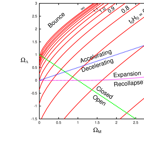
Figure 1: Parameter space $(\Omega_{M},\,\Omega_{\Lambda})$. The green (dashed) line $\Omega_{\Lambda}=1-\Omega_{M}$ corresponds to a flat universe, $\Omega_{K}=0$, separating open from closed universes. The blue (dotted) line $\Omega_{\Lambda}=\Omega_{M}/2$ corresponds to uniform expansion, $q_{0}=0$, separating accelerating from decelerating universes. The violet (dot-dashed) line corresponds to critical universes, separating eternal expansion from recollapse in the future. Finally, the red (continuous) lines correspond to $t_{0}H_{0}=0.5,\,0.6,\dots,\,\infty$, beyond which the universe has a bounce.

Moreover, different regions of this plane specify different behaviors of the universe. The boundaries between regions are well defined curves that can be computed for a given model. I will now describe the various regions and boundaries.

• Uniform expansion ($q_{0}=0$). Corresponds to the line $\Omega_{\Lambda}=\Omega_{M}/2$. Points above this line correspond to universes that are accelerating today, while those below correspond to decelerating universes, in particular the old cosmological model of Einstein-de Sitter (EdS), with $\Omega_{\Lambda}=0,\ \Omega_{M}=1$. Since 1998, all the data from Supernovae of type Ia appear above this line, many standard deviations away from EdS universes.

• Flat universe ($\Omega_{K}=0$). Corresponds to the line $\Omega_{\Lambda}=1-\Omega_{M}$. Points to the right of this line correspond to closed universes, while those to the left correspond to open ones. In the last few years we have mounting evidence that the universe is spatially flat (in fact Euclidean).

• Bounce ($t_{0}H_{0}=\infty$). Corresponds to a complicated function of $\Omega_{\Lambda}(\Omega_{M})$, normally expressed as an integral equation, where

  $$t_{0}H_{0}=\int_{0}^{1}da\ [1+\Omega_{M}(1/a-1)+\Omega_{\Lambda}(a^{2}-1)]^{-1/2}$$

  is the product of the age of the universe and the present rate of expansion. Points above this line correspond to universes that have contracted in the past and have later rebounced. At present, these universes are ruled out by observations of galaxies and quasars at high redshift (up to $z=10$).

• Critical Universe ($H=\dot{H}=0$). Corresponds to the boundary between eternal expansion in the future and recollapse. For $\Omega_{M}\leq 1$, it is simply the line $\Omega_{\Lambda}=0$, but for $\Omega_{M}>1$, it is a more complicated curve,

  $$\Omega_{\Lambda}=4\Omega_{M}\sin^{3}\Big{[}{1\over 3}\arcsin\Big{(}{\Omega_{M}-1\over\Omega_{M}}\Big{)}\Big{]}\simeq{4\over 27}{(\Omega_{M}-1)^{3}\over\Omega_{M}^{2}}.$$

  These critical solutions are asymptotic to the EdS model.

These boundaries, and the regions they delimit, can be seen in Fig. 1, together with the lines of equal $t_{0}H_{0}$ values.

In summary, the basic cosmological parameters that are now been hunted by a host of cosmological observations are the following: the present rate of expansion $H_{0}$; the age of the universe $t_{0}$; the deceleration parameter $q_{0}$; the spatial curvature $\Omega_{K}$; the matter content $\Omega_{M}$; the vacuum energy $\Omega_{\Lambda}$; the baryon density $\Omega_{B}$; the neutrino density $\Omega_{\nu}$, and many other that characterize the perturbations responsible for the large scale structure (LSS) and the CMB anisotropies.

3 The accelerating universe

Let us first describe the effect that the expansion of the universe has on the objects that live in it. In the absence of other forces but those of gravity, the trajectory of a particle is given by general relativity in terms of the geodesic equation

$${du^{\mu}\over ds}+\Gamma^{\mu}_{\nu\lambda}\,u^{\nu}u^{\lambda}=0\,,$$ (23)

where $u^{\mu}=(\gamma,\,\gamma v^{i})$, with $\gamma^{2}=1-v^{2}$ and $v^{i}$ is the peculiar velocity. Here $\Gamma^{\mu}_{\nu\lambda}$ is the Christoffel connection,[6] whose only non-zero component is $\Gamma^{0}_{ij}=(\dot{a}/a)\,g_{ij}$; substituting into the geodesic equation, we obtain $|\vec{u}|\propto 1/a$, and thus the particle’s momentum decays with the expansion like $p\propto 1/a$. In the case of a photon, satisfying the de Broglie relation $p=h/\lambda$, one obtains the well known photon redshift

$${\lambda_{1}\over\lambda_{0}}={a(t_{1})\over a(t_{0})}\ \ \Rightarrow\ \ z\equiv{\lambda_{0}-\lambda_{1}\over\lambda_{1}}={a_{0}\over a_{1}}-1\,,$$ (24)

where $\lambda_{0}$ is the wavelength measured by an observer at time $t_{0}$, while $\lambda_{1}$ is the wavelength emitted when the universe was younger $(t_{1}<t_{0})$. Normally we measure light from stars in distant galaxies and compare their observed spectra with our laboratory (restframe) spectra. The fraction (24) then gives the redshift $z$ of the object. We are assuming, of course, that both the emitted and the restframe spectra are identical, so that we can actually measure the effect of the intervening expansion, i.e. the growth of the scale factor from $t_{1}$ to $t_{0}$, when we compare the two spectra. Note that if the emitting galaxy and our own participated in the expansion, i.e. if our measuring rods (our rulers) also expanded with the universe, we would see no effect! The reason we can measure the redshift of light from a distant galaxy is because our galaxy is a gravitationally bounded object that has decoupled from the expansion of the universe. It is the distance between galaxies that changes with time, not the sizes of galaxies, nor the local measuring rods.

We can now evaluate the relationship between physical distance and redshift as a function of the rate of expansion of the universe. Because of homogeneity we can always choose our position to be at the origin $r=0$ of our spatial section. Imagine an object (a star) emitting light at time $t_{1}$, at coordinate distance $r_{1}$ from the origin. Because of isotropy we can ignore the angular coordinates $(\theta,\phi)$. Then the physical distance, to first order, will be $d=a_{0}\,r_{1}$. Since light travels along null geodesics,[6] we can write $0=-dt^{2}+a^{2}(t)\,dr^{2}/(1-Kr^{2})$, and therefore,

$$\int_{t_{1}}^{t_{0}}{dt\over a(t)}=\int_{0}^{r_{1}}{dr\over\sqrt{1-Kr^{2}}}\equiv f(r_{1})=\left\{\begin{array}[]{ll}\arcsin r_{1}&K=1\\ r_{1}&K=0\\ {\rm arcsinh}\,r_{1}&K=-1\end{array}\right.$$ (25)

If we now Taylor expand the scale factor to first order,

$${1\over 1+z}={a(t)\over a_{0}}=1+H_{0}(t-t_{0})+{\cal O}(t-t_{0})^{2}\,,$$ (26)

we find, to first approximation,

$$r_{1}\approx f(r_{1})={1\over a_{0}}(t_{0}-t_{1})+\dots={z\over a_{0}H_{0}}+\dots$$

Putting all together we find the famous Hubble law

$$H_{0}\,d=a_{0}H_{0}r_{1}=z\simeq vc\,,$$ (27)

which is just a kinematical effect (we have not included yet any dynamics, i.e. the matter content of the universe). Note that at low redshift $(z\ll 1)$, one is tempted to associate the observed change in wavelength with a Doppler effect due to a hypothetical recession velocity of the distant galaxy. This is only an approximation. In fact, the redshift cannot be ascribed to the relative velocity of the distant galaxy because in general relativity (i.e. in curved spacetimes) one cannot compare velocities through parallel transport, since the value depends on the path! If the distance to the galaxy is small, i.e. $z\ll 1$, the physical spacetime is not very different from Minkowsky and such a comparison is approximately valid. As $z$ becomes of order one, such a relation is manifestly false: galaxies cannot travel at speeds greater than the speed of light; it is the stretching of spacetime which is responsible for the observed redshift.

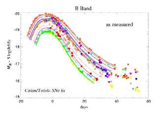
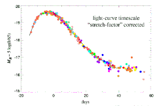
Figure 2: The Type Ia supernovae observed nearby show a relationship between their absolute luminosity and the timescale of their light curve: the brighter supernovae are slower and the fainter ones are faster. A simple linear relation between the absolute magnitude and a “stretch factor” multiplying the light curve timescale fits the data quite well.

Hubble’s law has been confirmed by observations ever since the 1920s, with increasing precision, which have allowed cosmologists to determine the Hubble parameter $H_{0}$ with less and less systematic errors. Nowadays, the best determination of the Hubble parameter was made by the Hubble Space Telescope Key Project,[7] $H_{0}=72\pm 8$ km/s/Mpc. This determination is based on objects at distances up to 500 Mpc, corresponding to redshifts $z\leq 0.1$.

Nowadays, we are beginning to probe much greater distances, corresponding to $z\simeq 1$, thanks to type Ia supernovae. These are white dwarf stars at the end of their life cycle that accrete matter from a companion until they become unstable and violently explode in a natural thermonuclear explosion that out-shines their progenitor galaxy. The intensity of the distant flash varies in time, it takes about three weeks to reach its maximum brightness and then it declines over a period of months. Although the maximum luminosity varies from one supernova to another, depending on their original mass, their environment, etc., there is a pattern: brighter explosions last longer than fainter ones. By studying the characteristic light curves, see Fig. 2, of a reasonably large statistical sample, cosmologists from the Supernova Cosmology Project[8] and the High-redshift Supernova Project,[9] are now quite confident that they can use this type of supernova as a standard candle. Since the light coming from some of these rare explosions has travelled a large fraction of the size of the universe, one expects to be able to infer from their distribution the spatial curvature and the rate of expansion of the universe. The connection between observations of high redshift supernovae and cosmological parameters is done via the luminosity distance, defined as the distance $d_{L}$ at which a source of absolute luminosity (energy emitted per unit time) ${\cal L}$ gives a flux (measured energy per unit time and unit area of the detector) ${\cal F}={\cal L}/4\pi\,d_{L}^{2}$. One can then evaluate, within a given cosmological model, the expression for $d_{L}$ as a function of redshift,[10]

$$H_{0}\,d_{L}(z)={(1+z)\over|\Omega_{K}|^{1/2}}\,{\rm sinn}\left[\int_{0}^{z}{|\Omega_{K}|^{1/2}\ dz^{\prime}\over\sqrt{(1+z^{\prime})^{2}(1+z^{\prime}\Omega_{M})-z^{\prime}(2+z^{\prime})\Omega_{\Lambda}}}\right]\,,$$ (28)

where ${\rm sinn}(x)=x\ {\rm if}\ K=0;\ \sin(x)\ {\rm if}\ K=+1\ {\rm and}\ \sinh(x)\ {\rm if}\ K=-1$, and we have used the cosmic sum rule (20).

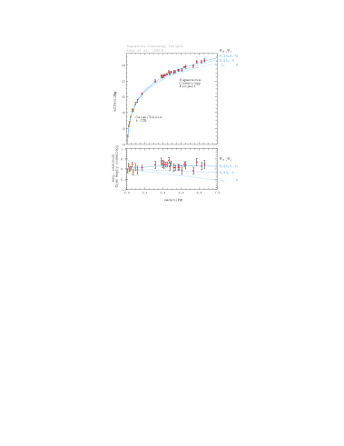
Figure 3: Upper panel: The Hubble diagram in linear redshift scale. Supernovae with $\Delta z<0.01$ of eachother have been weighted-averaged binned. The solid curve represents the best-fit flat universe model, $(\Omega_{M}=0.25,\,\Omega_{\Lambda}=0.75)$. Two other cosmological models are shown for comparison, $(\Omega_{M}=0.25,\,\Omega_{\Lambda}=0)$ and $(\Omega_{M}=1,\,\Omega_{\Lambda}=0)$. Lower panel: Residuals of the averaged data relative to an empty universe.

Astronomers measure the relative luminosity of a distant object in terms of what they call the effective magnitude, which has a peculiar relation with distance,

$$m(z)\equiv M+5\,\log_{10}\Big{[}{d_{L}(z)\over{\rm Mpc}}\Big{]}+25=\bar{M}+5\,\log_{10}[H_{0}\,d_{L}(z)]\,.$$ (29)

Since 1998, several groups have obtained serious evidence that high redshift supernovae appear fainter than expected for either an open $(\Omega_{M}<1)$ or a flat $(\Omega_{M}=1)$ universe, see Fig. 3. In fact, the universe appears to be accelerating instead of decelerating, as was expected from the general attraction of matter, see Eq. (22); something seems to be acting as a repulsive force on very large scales. The most natural explanation for this is the presence of a cosmological constant, a diffuse vacuum energy that permeates all space and, as explained above, gives the universe an acceleration that tends to separate gravitationally bound systems from each other. The best-fit results from the Supernova Cosmology Project[11] give a linear combination

$$0.8\Omega_{M}-0.6\Omega_{\Lambda}=-0.16\pm 0.05\ \ (1\sigma),$$

which is now many sigma away from an EdS model with $\Lambda=0$. In particular, for a flat universe this gives

$$\Omega_{\Lambda}=0.71\pm 0.05\hskip 28.45274pt{\rm and}\hskip 28.45274pt\Omega_{M}=0.29\pm 0.05\ \ (1\sigma).$$

Surprising as it may seem, arguments for a significant dark energy component of the universe where proposed long before these observations, in order to accommodate the ages of globular clusters, as well as a flat universe with a matter content below critical, which was needed in order to explain the observed distribution of galaxies, clusters and voids.

Taylor expanding the scale factor to third order,

$${a(t)\over a_{0}}=1+H_{0}(t-t_{0})-{q_{0}\over 2!}H_{0}^{2}(t-t_{0})^{2}+{j_{0}\over 3!}H_{0}^{3}(t-t_{0})^{3}+{\cal O}(t-t_{0})^{4}\,,$$ (30)

where

$$q_{0}=-\,{\ddot{a}\over aH^{2}}(t_{0})={1\over 2}\sum_{i}(1+3w_{i})\Omega_{i}={1\over 2}\Omega_{M}-\Omega_{\Lambda}\,,$$ (31)

$$j_{0}=+\,{\stackrel{{\scriptstyle\dots}}{{a}}\over aH^{3}}(t_{0})={1\over 2}\sum_{i}(1+3w_{i})(2+3w_{i})\Omega_{i}=\Omega_{M}+\Omega_{\Lambda}\,,$$ (32)

are the deceleration and “jerk” parameters. Substituting into Eq. (28) we find

$$H_{0}\,d_{L}(z)=z+{1\over 2}(1-q_{0})\,z^{2}-{1\over 6}(1-q_{0}-3q_{0}^{2}+j_{0})\,z^{3}+{\cal O}(z^{4})\,.$$ (33)

This expression goes beyond the leading linear term, corresponding to the Hubble law, into the second and third order terms, which are sensitive to the cosmological parameters $\Omega_{M}$ and $\Omega_{\Lambda}$. It is only recently that cosmological observations have gone far enough back into the early universe that we can begin to probe these terms, see Fig. 4.

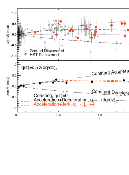
Figure 4: The Supernovae Ia residual Hubble diagram. Upper panel: Ground-based discoveries are represented by diamonds, HST-discovered SNe Ia are shown as filled circles. Lower panel: The same but with weighted averaged in fixed redshift bins. Kinematic models of the expansion history are shown relative to an eternally coasting model $q(z)=0$.

This extra component of the critical density would have to resist gravitational collapse, otherwise it would have been detected already as part of the energy in the halos of galaxies. However, if most of the energy of the universe resists gravitational collapse, it is impossible for structure in the universe to grow. This dilemma can be resolved if the hypothetical dark energy was negligible in the past and only recently became the dominant component. According to general relativity, this requires that the dark energy have negative pressure, since the ratio of dark energy to matter density goes like $a(t)^{-3p/\rho}$. This argument would rule out almost all of the usual suspects, such as cold dark matter, neutrinos, radiation, and kinetic energy, since they all have zero or positive pressure. Thus, we expect something like a cosmological constant, with a negative pressure, $p\approx-\rho$, to account for the missing energy.

However, if the universe was dominated by dark matter in the past, in order to form structure, and only recently became dominated by dark energy, we must be able to see the effects of the transition from the deceleration into the acceleration phase in the luminosity of distant type Ia supernovae. This has been searched for since 1998, when the first convincing results on the present acceleration appeared. However, only recently[12] do we have clear evidence of this transition point in the evolution of the universe. This coasting point is defined as the time, or redshift, at which the deceleration parameter vanishes,

$$q(z)=-1+(1+z)\,{d\over dz}\ln H(z)=0\,,$$ (34)

where

$$H(z)=H_{0}\Big{[}\Omega_{M}(1+z)^{3}+\Omega_{x}\,e^{3\int_{0}^{z}(1+w_{x}(z^{\prime})){dz^{\prime}\over 1+z^{\prime}}}\ +\Omega_{K}(1+z)^{2}\Big{]}^{1/2}\,,$$ (35)

and we have assumed that the dark energy is parametrized by a density $\Omega_{x}$ today, with a redshift-dependent equation of state, $w_{x}(z)$, not necessarily equal to $-1$. Of course, in the case of a true cosmological constant, this reduces to the usual expression.

Figure 5: The recent supernovae data on the $(\Omega_{M},\,\Omega_{\Lambda})$ plane, see Ref. [12]. Shown are the 1-, 2- and 3-$\sigma$ contours, as well as the data from 1998, for comparison. It is clear that the old EdS cosmological model at $(\Omega_{M}=1,\,\Omega_{\Lambda}=0)$ is many standard deviations away from the data.

Let us suppose for a moment that the barotropic parameter $w$ is constant, then the coasting redshift can be determined from

$$q(z)={1\over 2}\Big{[}{\Omega_{M}+(1+3w)\,\Omega_{x}\,(1+z)^{3w}\over\Omega_{M}+\Omega_{x}\,(1+z)^{3w}+\Omega_{K}(1+z)^{-1}}\Big{]}=0\,,$$ (36)

$$\hskip 28.45274pt\Rightarrow z_{c}=\left({(3|w|-1)\Omega_{x}\over\Omega_{M}}\right)^{1\over 3|w|}-1\,,$$ (37)

which, in the case of a true cosmological constant, reduces to

$$z_{c}=\Big{(}{2\Omega_{\Lambda}\over\Omega_{M}}\Big{)}^{1/3}-1\,.$$ (38)

When substituting $\Omega_{\Lambda}\simeq 0.7$ and $\Omega_{M}\simeq 0.3$, one obtains $z_{c}\simeq 0.6$, in excellent agreement with recent observations.[12] The plane $(\Omega_{M},\,\Omega_{\Lambda})$ can be seen in Fig. 5, which shows a significant improvement with respect to previous data.

Now, if we have to live with this vacuum energy, we might as well try to comprehend its origin. For the moment it is a complete mystery, perhaps the biggest mystery we have in physics today. We measure its value but we don’t understand why it has the value it has. In fact, if we naively predict it using the rules of quantum mechanics, we find a number that is many (many!) orders of magnitude off the mark. Let us describe this calculation in some detail. In non-gravitational physics, the zero-point energy of the system is irrelevant because forces arise from gradients of potential energies. However, we know from general relativity that even a constant energy density gravitates. Let us write down the most general energy momentum tensor compatible with the symmetries of the metric and that is covariantly conserved. This is precisely of the form $T_{\mu\nu}^{(vac)}=p_{V}\,g_{\mu\nu}=-\,\rho_{V}\,g_{\mu\nu}$. Substituting into the Einstein equations (1), we see that the cosmological constant and the vacuum energy are completely equivalent, $\Lambda=8\pi G\,\rho_{V}$, so we can measure the vacuum energy with the observations of the acceleration of the universe, which tells us that $\Omega_{\Lambda}\simeq 0.7$.

On the other hand, we can estimate the contribution to the vacuum energy coming from the quantum mechanical zero-point energy of the quantum oscillators associated with the fluctuations of all quantum fields,

$$\rho_{V}^{th}=\sum_{i}\int_{0}^{\Lambda_{UV}}\!\!{d^{2}k\over(2\pi)^{3}}\,{1\over 2}\hbar\omega_{i}(k)={\hbar\Lambda_{UV}^{4}\over 16\pi^{2}}\sum_{i}(-1)^{F}N_{i}+{\cal O}(m_{i}^{2}\Lambda_{UV}^{2})\,,$$ (39)

where $\Lambda_{UV}$ is the ultraviolet cutoff signaling the scale of new physics. Taking the scale of quantum gravity, $\Lambda_{UV}=M_{Pl}$, as the cutoff, and barring any fortuituous cancellations, then the theoretical expectation (39) appears to be 120 orders of magnitude larger than the observed vacuum energy associated with the acceleration of the universe,

$$\rho_{V}^{th}\simeq 1.4\times 10^{74}\ {\rm GeV}^{4}=3.2\times 10^{91}\ {\rm g/cm}^{3}\,,$$ (40)

$$\rho_{V}^{obs}\simeq 0.7\,\rho_{c}=0.66\times 10^{-29}\ {\rm g/cm}^{3}=2.9\times 10^{-11}\ {\rm eV}^{4}\,.$$ (41)

Even if we assumed that the ultraviolet cutoff associated with quantum gravity was as low as the electroweak scale (and thus around the corner, liable to be explored in the LHC), the theoretical expectation would still be 60 orders of magnitude too bit. This is by far the worst mismatch between theory and observations in all of science. There must be something seriously wrong in our present understanding of gravity at the most fundamental level. Perhaps we don’t understand the vacuum and its energy does not gravitate after all, or perhaps we need to impose a new principle (or a symmetry) at the quantum gravity level to accommodate such a flagrant mismatch.

In the meantime, one can at least parametrize our ignorance by making variations on the idea of a constant vacuum energy. Let us assume that it actually evolves slowly with time. In that case, we do not expect the equation of state $p=-\rho$ to remain true, but instead we expect the barotropic parameter $w(z)$ to depend on redshift. Such phenomenological models have been proposed, and until recently produced results that were compatible with $w=-1$ today, but with enough uncertainty to speculate on alternatives to a truly constant vacuum energy. However, with the recent supernovae results,[12] there seems to be little space for variations, and models of a time-dependent vacuum energy are less and less favoured. In the near future, the SNAP satellite[13] will measure several thousand supernovae at high redshift and therefore map the redshift dependence of both the dark energy density and its equation of state with great precision. This will allow a much better determination of the cosmological parameters $\Omega_{M}$ and $\Omega_{\Lambda}$.

4 Dark Matter

In the 1920s Hubble realized that the so called nebulae were actually distant galaxies very similar to our own. Soon afterwards, in 1933, Zwicky found dynamical evidence that there is possibly ten to a hundred times more mass in the Coma cluster than contributed by the luminous matter in galaxies.[14] However, it was not until the 1970s that the existence of dark matter began to be taken more seriously. At that time there was evidence that rotation curves of galaxies did not fall off with radius and that the dynamical mass was increasing with scale from that of individual galaxies up to clusters of galaxies. Since then, new possible extra sources to the matter content of the universe have been accumulating:

$$\Omega_{M} = \Omega_{B,\ {\rm lum}}\hskip 25.6073pt({\rm stars\ in\ galaxies})$$ (42)

$$+ \Omega_{B,\ {\rm dark}}\hskip 22.76228pt({\rm MACHOs?})$$ (43)

$$+ \Omega_{CDM}\hskip 28.45274pt({\rm weakly\ interacting:\ axion,\ neutralino?})$$ (44)

$$+ \Omega_{HDM}\hskip 28.45274pt({\rm massive\ neutrinos?})$$ (45)

The empirical route to the determination of $\Omega_{M}$ is nowadays one of the most diversified of all cosmological parameters. The matter content of the universe can be deduced from the mass-to-light ratio of various objects in the universe; from the rotation curves of galaxies; from microlensing and the direct search of Massive Compact Halo Objects (MACHOs); from the cluster velocity dispersion with the use of the Virial theorem; from the baryon fraction in the X-ray gas of clusters; from weak gravitational lensing; from the observed matter distribution of the universe via its power spectrum; from the cluster abundance and its evolution; from direct detection of massive neutrinos at SuperKamiokande; from direct detection of Weakly Interacting Massive Particles (WIMPs) at DAMA and UKDMC, and finally from microwave background anisotropies. I will review here just a few of them.

4.1 Rotation curves of spiral galaxies

The flat rotation curves of spiral galaxies provide the most direct evidence for the existence of large amounts of dark matter. Spiral galaxies consist of a central bulge and a very thin disk, stabilized against gravitational collapse by angular momentum conservation, and surrounded by an approximately spherical halo of dark matter. One can measure the orbital velocities of objects orbiting around the disk as a function of radius from the Doppler shifts of their spectral lines.

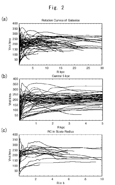
Figure 6: The rotation curves of several hundred galaxies. Upper panel: As a function of their radii in kpc. Middle panel: The central 5 kpc. Lower panel: As a function of scale radius.

The rotation curve of the Andromeda galaxy was first measured by Babcock in 1938, from the stars in the disk. Later it became possible to measure galactic rotation curves far out into the disk, and a trend was found.[15] The orbital velocity rose linearly from the center outward until it reached a typical value of 200 km/s, and then remained flat out to the largest measured radii. This was completely unexpected since the observed surface luminosity of the disk falls off exponentially with radius,[15] $I(r)=I_{0}\exp(-r/r_{D})$. Therefore, one would expect that most of the galactic mass is concentrated within a few disk lengths $r_{D}$, such that the rotation velocity is determined as in a Keplerian orbit, $v_{\rm rot}=(GM/r)^{1/2}\propto r^{-1/2}$. No such behaviour is observed. In fact, the most convincing observations come from radio emission (from the 21 cm line) of neutral hydrogen in the disk, which has been measured to much larger galactic radii than optical tracers. A typical case is that of the spiral galaxy NGC 6503, where $r_{D}=1.73$ kpc, while the furthest measured hydrogen line is at $r=22.22$ kpc, about 13 disk lengths away. Nowadays, thousands of galactic rotation curves are known, see Fig. 6, and all suggest the existence of about ten times more mass in the halos of spiral galaxies than in the stars of the disk. Recent numerical simulations of galaxy formation in a CDM cosmology[16] suggest that galaxies probably formed by the infall of material in an overdense region of the universe that had decoupled from the overall expansion. The dark matter is supposed to undergo violent relaxation and create a virialized system, i.e. in hydrostatic equilibrium. This picture has led to a simple model of dark-matter halos as isothermal spheres, with density profile $\rho(r)=\rho_{c}/(r_{c}^{2}+r^{2})$, where $r_{c}$ is a core radius and $\rho_{c}=v_{\infty}^{2}/4\pi G$, with $v_{\infty}$ equal to the plateau value of the flat rotation curve. This model is consistent with the universal rotation curves seen in Fig. 6. At large radii the dark matter distribution leads to a flat rotation curve. The question is for how long. In dense galaxy clusters one expects the galactic halos to overlap and form a continuum, and therefore the rotation curves should remain flat from one galaxy to another. However, in field galaxies, far from clusters, one can study the rotation velocities of substructures (like satellite dwarf galaxies) around a given galaxy, and determine whether they fall off at sufficiently large distances according to Kepler’s law, as one would expect, once the edges of the dark matter halo have been reached. These observations are rather difficult because of uncertainties in distinguishing between true satellites and interlopers. Recently, a group from the Sloan Digital Sky Survey Collaboration claim that they have seen the edges of the dark matter halos around field galaxies by confirming the fall-off at large distances of their rotation curves.[17] These results, if corroborated by further analysis, would constitute a tremendous support to the idea of dark matter as a fluid surrounding galaxies and clusters, while at the same time eliminates the need for modifications of Newtonian of even Einstenian gravity at the scales of galaxies, to account for the flat rotation curves.

That’s fine, but how much dark matter is there at the galactic scale? Adding up all the matter in galactic halos up to a maximum radii, one finds

$$\Omega_{\rm halo}\simeq 10\ \Omega_{\rm lum}\geq 0.03-0.05\,.$$ (46)

Of course, it would be extraordinary if we could confirm, through direct detection, the existence of dark matter in our own galaxy. For that purpose, one should measure its rotation curve, which is much more difficult because of obscuration by dust in the disk, as well as problems with the determination of reliable galactocentric distances for the tracers. Nevertheless, the rotation curve of the Milky Way has been measured and conforms to the usual picture, with a plateau value of the rotation velocity of 220 km/s. For dark matter searches, the crucial quantity is the dark matter density in the solar neighbourhood, which turns out to be (within a factor of two uncertainty depending on the halo model) $\rho_{\rm DM}=0.3$ GeV/cm³. We will come back to direct searched of dark matter in a later subsection.

4.2 Baryon fraction in clusters

Since large clusters of galaxies form through gravitational collapse, they scoop up mass over a large volume of space, and therefore the ratio of baryons over the total matter in the cluster should be representative of the entire universe, at least within a 20% systematic error. Since the 1960s, when X-ray telescopes became available, it is known that galaxy clusters are the most powerful X-ray sources in the sky.[18] The emission extends over the whole cluster and reveals the existence of a hot plasma with temperature $T\sim 10^{7}-10^{8}$ K, where X-rays are produced by electron bremsstrahlung. Assuming the gas to be in hydrostatic equilibrium and applying the virial theorem one can estimate the total mass in the cluster, giving general agreement (within a factor of 2) with the virial mass estimates. From these estimates one can calculate the baryon fraction of clusters

$$f_{\rm B}h^{3/2}=0.08\hskip 14.22636pt\Rightarrow\hskip 14.22636pt{\Omega_{B}\over\Omega_{M}}\approx 0.14\,,\hskip 14.22636pt{\rm for}\hskip 8.53581pth=0.70\,.$$ (47)

Since $\Omega_{\rm lum}\simeq 0.002-0.006$, the previous expression suggests that clusters contain far more baryonic matter in the form of hot gas than in the form of stars in galaxies. Assuming this fraction to be representative of the entire universe, and using the Big Bang nucleosynthesis value of $\Omega_{B}=0.04\pm 0.01$, for $h=0.7$, we find

$$\Omega_{M}=0.3\pm 0.1\ ({\rm statistical})\ \pm 20\%\ ({\rm systematic})\,.$$ (48)

This value is consistent with previous determinations of $\Omega_{M}$. If some baryons are ejected from the cluster during gravitational collapse, or some are actually bound in nonluminous objects like planets, then the actual value of $\Omega_{M}$ is smaller than this estimate.

4.3 Weak gravitational lensing

Since the mid 1980s, deep surveys with powerful telescopes have observed huge arc-like features in galaxy clusters. The spectroscopic analysis showed that the cluster and the giant arcs were at very different redshifts. The usual interpretation is that the arc is the image of a distant background galaxy which is in the same line of sight as the cluster so that it appears distorted and magnified by the gravitational lens effect: the giant arcs are essentially partial Einstein rings. From a systematic study of the cluster mass distribution one can reconstruct the shear field responsible for the gravitational distortion.[19] This analysis shows that there are large amounts of dark matter in the clusters, in rough agreement with the virial mass estimates, although the lensing masses tend to be systematically larger. At present, the estimates indicate $\Omega_{M}=0.2-0.3$ on scales $\mathrel{\mathop{\hbox{\lower 2.15277pt\hbox{$\sim$}\kern-8.00003pt\lower-3.01385pt\hbox{$<$}}}}6\,h^{-1}$ Mpc.

4.4 Large scale structure formation and the matter power spectrum

Although the isotropic microwave background indicates that the universe in the past was extraordinarily homogeneous, we know that the universe today is far from homogeneous: we observe galaxies, clusters and superclusters on large scales. These structures are expected to arise from very small primordial inhomogeneities that grow in time via gravitational instability, and that may have originated from tiny ripples in the metric, as matter fell into their troughs. Those ripples must have left some trace as temperature anisotropies in the microwave background, and indeed such anisotropies were finally discovered by the COBE satellite in 1992. However, not all kinds of matter and/or evolution of the universe can give rise to the structure we observe today. If we define the density contrast as

$$\delta(\vec{x},a)\equiv{\rho(\vec{x},a)-\bar{\rho}(a)\over\bar{\rho}(a)}=\int d^{3}\vec{k}\ \delta_{k}(a)\ e^{i\vec{k}\cdot\vec{x}}\,,$$ (49)

where $\bar{\rho}(a)=\rho_{0}\,a^{-3}$ is the average cosmic density, we need a theory that will grow a density contrast with amplitude $\delta\sim 10^{-5}$ at the last scattering surface ($z=1100$) up to density contrasts of the order of $\delta\sim 10^{2}$ for galaxies at redshifts $z\ll 1$, i.e. today. This is a necessary requirement for any consistent theory of structure formation.

Furthermore, the anisotropies observed by the COBE satellite correspond to a small-amplitude scale-invariant primordial power spectrum of inhomogeneities

$$P(k)=\langle|\delta_{k}|^{2}\rangle\propto k^{n}\,,\hskip 14.22636pt{\rm with}\hskip 14.22636ptn=1\,,$$ (50)

These inhomogeneities are like waves in the space-time metric. When matter fell in the troughs of those waves, it created density perturbations that collapsed gravitationally to form galaxies and clusters of galaxies, with a spectrum that is also scale invariant. Such a type of spectrum was proposed in the early 1970s by Edward R. Harrison, and independently by the Russian cosmologist Yakov B. Zel’dovich,[20] to explain the distribution of galaxies and clusters of galaxies on very large scales in our observable universe.

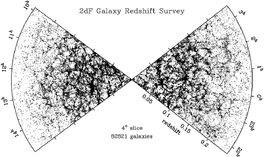
Figure 7: The 2 degree Field Galaxy Redshift Survey contains some 250,000 galaxies, covering a large fraction of the sky up to redshifts of $z\leq 0.25$.

Since the primordial spectrum is very approximately represented by a scale-invariant Gaussian random field, the best way to present the results of structure formation is by working with the 2-point correlation function in Fourier space, the so-called power spectrum. If the reprocessed spectrum of inhomogeneities remains Gaussian, the power spectrum is all we need to describe the galaxy distribution. Non-Gaussian effects are expected to arise from the non-linear gravitational collapse of structure, and may be important at small scales. The power spectrum measures the degree of inhomogeneity in the mass distribution on different scales. It depends upon a few basic ingredientes: a) the primordial spectrum of inhomogeneities, whether they are Gaussian or non-Gaussian, whether adiabatic (perturbations in the energy density) or isocurvature (perturbations in the entropy density), whether the primordial spectrum has tilt (deviations from scale-invariance), etc.; b) the recent creation of inhomogeneities, whether cosmic strings or some other topological defect from an early phase transition are responsible for the formation of structure today; and c) the cosmic evolution of the inhomogeneity, whether the universe has been dominated by cold or hot dark matter or by a cosmological constant since the beginning of structure formation, and also depending on the rate of expansion of the universe.

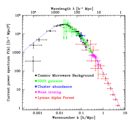
Figure 8: The measured power spectrum $P(k)$ as a function of wavenumber $k$. From observations of the Sloan Digital Sky Survey, CMB anisotropies, cluster abundance, gravitational lensing and Lyman-$\alpha$ forest.

The working tools used for the comparison between the observed power spectrum and the predicted one are very precise N-body numerical simulations and theoretical models that predict the shape but not the amplitude of the present power spectrum. Even though a large amount of work has gone into those analyses, we still have large uncertainties about the nature and amount of matter necessary for structure formation. A model that has become a working paradigm is a flat cold dark matter model with a cosmological constant and $\Omega_{M}\sim 0.3$. This model is now been confronted with the recent very precise measurements from 2dFGRS[21] and SDSS.[22]

4.5 The new redshift catalogs, 2dF and Sloan Digital Sky Survey

Our view of the large-scale distribution of luminous objects in the universe has changed dramatically during the last 25 years: from the simple pre-1975 picture of a distribution of field and cluster galaxies, to the discovery of the first single superstructures and voids, to the most recent results showing an almost regular web-like network of interconnected clusters, filaments and walls, separating huge nearly empty volumes. The increased efficiency of redshift surveys, made possible by the development of spectrographs and – specially in the last decade – by an enormous increase in multiplexing gain (i.e. the ability to collect spectra of several galaxies at once, thanks to fibre-optic spectrographs), has allowed us not only to do cartography of the nearby universe, but also to statistically characterize some of its properties. At the same time, advances in theoretical modeling of the development of structure, with large high-resolution gravitational simulations coupled to a deeper yet limited understanding of how to form galaxies within the dark matter halos, have provided a more realistic connection of the models to the observable quantities. Despite the large uncertainties that still exist, this has transformed the study of cosmology and large-scale structure into a truly quantitative science, where theory and observations can progress together.

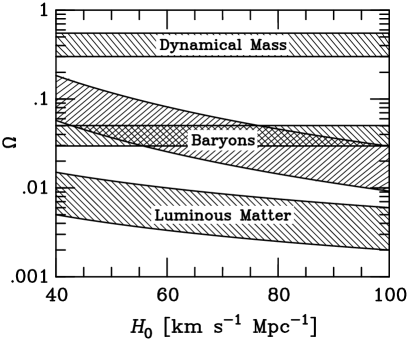
Figure 9: The observed cosmic matter components as functions of the Hubble expansion parameter. The luminous matter component is given by $0.002\leq\Omega_{\rm lum}\leq 0.006$; the galactic halo component is the horizontal band, $0.03\leq\Omega_{\rm halo}\leq 0.05$, crossing the baryonic component from BBN, $\Omega_{B}\,h^{2}=0.0244\pm 0.0024$; and the dynamical mass component from large scale structure analysis is given by $\Omega_{M}=0.3\pm 0.1$. Note that in the range $H_{0}=70\pm 7$ km/s/Mpc, there are three dark matter problems, see the text.

4.6 Summary of the matter content

We can summarize the present situation with Fig. 9, for $\Omega_{M}$ as a function of $H_{0}$. There are four bands, the luminous matter $\Omega_{\rm lum}$; the baryon content $\Omega_{B}$, from BBN; the galactic halo component $\Omega_{\rm halo}$, and the dynamical mass from clusters, $\Omega_{M}$. From this figure it is clear that there are in fact three dark matter problems: The first one is where are 90% of the baryons? Between the fraction predicted by BBN and that seen in stars and diffuse gas there is a huge fraction which is in the form of dark baryons. They could be in small clumps of hydrogen that have not started thermonuclear reactions and perhaps constitute the dark matter of spiral galaxies’ halos. Note that although $\Omega_{B}$ and $\Omega_{\rm halo}$ coincide at $H_{0}\simeq 70$ km/s/Mpc, this could be just a coincidence. The second problem is what constitutes 90% of matter, from BBN baryons to the mass inferred from cluster dynamics? This is the standard dark matter problem and could be solved in the future by direct detection of a weakly interacting massive particle in the laboratory. And finally, since we know from observations of the CMB that the universe is flat, the rest, up to $\Omega_{0}=1$, must be a diffuse vacuum energy, which affects the very large scales and late times, and seems to be responsible for the present acceleration of the universe, see Section 3.

5 The anisotropies of the microwave background

One of the most remarkable observations ever made my mankind is the detection of the relic background of photons from the Big Bang. This background was predicted by George Gamow and collaborators in the 1940s, based on the consistency of primordial nucleosynthesis with the observed helium abundance. They estimated a value of about 10 K, although a somewhat more detailed analysis by Alpher and Herman in 1950 predicted $T_{\gamma}\approx 5$ K. Unfortunately, they had doubts whether the radiation would have survived until the present, and this remarkable prediction slipped into obscurity, until Dicke, Peebles, Roll and Wilkinson studied the problem again in 1965.[23] Before they could measure the photon background, they learned that Penzias and Wilson had observed a weak isotropic background signal at a radio wavelength of 7.35 cm, corresponding to a blackbody temperature of $T_{\gamma}=3.5\pm 1$ K. They published their two papers back to back, with that of Dicke et al. explaining the fundamental significance of their measurement.

Since then many different experiments have confirmed the existence of the microwave background. The most outstanding one has been the Cosmic Background Explorer (COBE) satellite, whose FIRAS instrument measured the photon background with great accuracy over a wide range of frequencies. Nowadays, the photon spectrum is confirmed to be a blackbody spectrum with a temperature[24]

$$T_{{}_{\rm CMB}}=2.728\pm 0.002\ {\rm K}\ ({\rm systematic},\ 95\%\ {\rm c.l.})\ \pm 7\ \mu\!{\rm K}\ (1\sigma\ {\rm statistical})$$ (51)

In fact, this is the best blackbody spectrum ever measured, with spectral distortions below the level of 10 parts per million (ppm). Moreover, the differential microwave radiometer (DMR) instrument on COBE, with a resolution of about $7^{\circ}$ in the sky, has also confirmed that it is an extraordinarily isotropic background.[25] The deviations from isotropy, i.e. differences in the temperature of the blackbody spectrum measured in different directions in the sky, are of the order of 20 $\mu$K on large scales, or one part in $10^{5}$. Soon after COBE, other groups quickly confirmed the detection of temperature anisotropies at around 30 $\mu$K and above, at higher multipole numbers or smaller angular scales. Last year, the satellite Wilkinson Microwave Anisotropy Probe (WMAP)[26] measured the full sky CMB anisotropies with 10 arcminutes’ resolution, and obtained the most precise map to date of the microwave sky, see Fig. 10

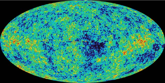
Figure 10: The anisotropies of the microwave background measured by the WMAP satellite with 10 arcminute resolution. It shows the intrinsic CMB anisotropies at the level of a few parts in $10^{5}$. The galactic foreground has been properly subtracted. The amount of information contained in this map is enough to determine most of the cosmological parameters to few percent accuracy.

5.1 Acoustic oscillations in the plasma before recombination

The physics of the CMB anisotropies is relatively simple.[27] The universe just before recombination is a very tightly coupled fluid, due to the large electromagnetic Thomson cross section $\sigma_{T}=8\pi\alpha^{2}/3m_{e}^{2}\simeq 0.7$ barn. Photons scatter off charged particles (protons and electrons), and carry energy, so they feel the gravitational potential associated with the perturbations imprinted in the metric during inflation. An overdensity of baryons (protons and neutrons) does not collapse under the effect of gravity until it enters the causal Hubble radius. The perturbation continues to grow until radiation pressure opposes gravity and sets up acoustic oscillations in the plasma, very similar to sound waves. Since overdensities of the same size will enter the Hubble radius at the same time, they will oscillate in phase. Moreover, since photons scatter off these baryons, the acoustic oscillations occur also in the photon field and induces a pattern of peaks in the temperature anisotropies in the sky, at different angular scales, see Fig. 11.

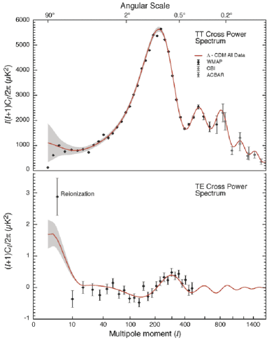
Figure 11: The Angular Power Spectrum of CMB temperature anisotropies, compared with the cross-correlation of temperature-polarization anisotropies.

There are three different effects that determine the temperature anisotropies we observe in the CMB. First, gravity: photons fall in and escape off gravitational potential wells, characterized by $\Phi$ in the comoving gauge, and as a consequence their frequency is gravitationally blue- or red-shifted, $\delta\nu/\nu=\Phi$. If the gravitational potential is not constant, the photons will escape from a larger or smaller potential well than they fell in, so their frequency is also blue- or red-shifted, a phenomenon known as the Rees-Sciama effect. Second, pressure: photons scatter off baryons which fall into gravitational potential wells and the two competing forces create acoustic waves of compression and rarefaction. Finally, velocity: baryons accelerate as they fall into potential wells. They have minimum velocity at maximum compression and rarefaction. That is, their velocity wave is exactly $90^{\circ}$ off-phase with the acoustic waves. These waves induce a Doppler effect on the frequency of the photons. The temperature anisotropy induced by these three effects is therefore given by[27]

$${\delta T\over T}({\bf r})=\Phi({\bf r},t_{\rm dec})+2\int_{t_{\rm dec}}^{t_{0}}\dot{\Phi}({\bf r},t)dt\ +\ {1\over 3}{\delta\rho\over\rho}\ -\ {{\bf r}\cdot{\bf v}\over c}\,.$$ (52)

Metric perturbations of different wavelengths enter the horizon at different times. The largest wavelengths, of size comparable to our present horizon, are entering now. There are perturbations with wavelengths comparable to the size of the horizon at the time of last scattering, of projected size about $1^{\circ}$ in the sky today, which entered precisely at decoupling. And there are perturbations with wavelengths much smaller than the size of the horizon at last scattering, that entered much earlier than decoupling, all the way to the time of radiation-matter equality, which have gone through several acoustic oscillations before last scattering. All these perturbations of different wavelengths leave their imprint in the CMB anisotropies.

The baryons at the time of decoupling do not feel the gravitational attraction of perturbations with wavelength greater than the size of the horizon at last scattering, because of causality. Perturbations with exactly that wavelength are undergoing their first contraction, or acoustic compression, at decoupling. Those perturbations induce a large peak in the temperature anisotropies power spectrum, see Fig. 11. Perturbations with wavelengths smaller than these will have gone, after they entered the Hubble scale, through a series of acoustic compressions and rarefactions, which can be seen as secondary peaks in the power spectrum. Since the surface of last scattering is not a sharp discontinuity, but a region of $\Delta z\sim 100$, there will be scales for which photons, travelling from one energy concentration to another, will erase the perturbation on that scale, similarly to what neutrinos or HDM do for structure on small scales. That is the reason why we don’t see all the acoustic oscillations with the same amplitude, but in fact they decay exponentialy towards smaller angular scales, an effect known as Silk damping, due to photon diffusion.[27]

Table 1: The parameters of the standard cosmological model. The standard model of cosmology has about 20 different parameters, needed to describe the background space-time, the matter content and the spectrum of metric perturbations. We include here the present range of the most relevant parameters (with 1$\sigma$ errors), as recently determined by WMAP, and the error with which the Planck satellite will be able to determine them in the near future. The rate of expansion is written in units of $H=100\,h$ km/s/Mpc

physical quantity	symbol	WMAP	Planck
total density	$\Omega_{0}$	$1.02\pm 0.02$	0.7%
baryonic matter	$\Omega_{\rm B}$	$0.044\pm 0.004$	0.6%
cosmological constant	$\Omega_{\Lambda}$	$0.73\pm 0.04$	0.5%
cold dark matter	$\Omega_{\rm M}$	$0.23\pm 0.04$	0.6%
hot dark matter	$\Omega_{\nu}h^{2}$	$<0.0076$ (95% c.l.)	1%
sum of neutrino masses	$\sum m_{\nu}$ (eV)	$<0.23$ (95% c.l.)	1%
CMB temperature	$T_{0}\ (K)$	$2.725\pm 0.002$	0.1%
baryon to photon ratio	$\eta\times 10^{10}$	$6.1\pm 0.3$	0.5%
baryon to matter ratio	$\Omega_{\rm B}/\Omega_{\rm M}$	$0.17\pm 0.01$	1%
spatial curvature	$\Omega_{K}$	$<0.02$ (95% c.l.)	0.5%
rate of expansion	$h$	$0.71\pm 0.03$	0.8%
age of the universe	$t_{0}$ (Gyr)	$13.7\pm 0.2$	0.1%
age at decoupling	$t_{\rm dec}$ (kyr)	$379\pm 8$	0.5%
age at reionization	$t_{\rm r}$ (Myr)	$180\pm 100$	5%
spectral amplitude	$A$	$0.833\pm 0.085$	0.1%
spectral tilt	$n_{\rm s}$	$0.95\pm 0.03$	0.2%
spectral tilt variation	$dn_{\rm s}/d\ln k$	$-0.031\pm 0.017$	0.5%
tensor-scalar ratio	$r$	$<0.71$ (95% c.l.)	5%
reionization optical depth	$\tau$	$0.17\pm 0.04$	5%
redshift of equality	$z_{\rm eq}$	$3233\pm 200$	5%
redshift of decoupling	$z_{\rm dec}$	$1089\pm 1$	0.1%
width of decoupling	$\Delta z_{\rm dec}$	$195\pm 2$	1%
redshift of reionization	$z_{\rm r}$	$20\pm 10$	2%

From the observations of the CMB anisotropies it is possible to determine most of the parameters of the Standard Cosmological Model with few percent accuracy, see Table 1. However, there are many degeneracies between parameters and it is difficult to disentangle one from another. For instance, as mentioned above, the first peak in the photon distribution corresponds to overdensities that have undergone half an oscillation, that is, a compression, and appear at a scale associated with the size of the horizon at last scattering, about $1^{\circ}$ projected in the sky today. Since photons scatter off baryons, they will also feel the acoustic wave and create a peak in the correlation function. The height of the peak is proportional to the amount of baryons: the larger the baryon content of the universe, the higher the peak. The position of the peak in the power spectrum depends on the geometrical size of the particle horizon at last scattering. Since photons travel along geodesics, the projected size of the causal horizon at decoupling depends on whether the universe is flat, open or closed. In a flat universe the geodesics are straight lines and, by looking at the angular scale of the first acoustic peak, we would be measuring the actual size of the horizon at last scattering. In an open universe, the geodesics are inward-curved trajectories, and therefore the projected size on the sky appears smaller. In this case, the first acoustic peak should occur at higher multipoles or smaller angular scales. On the other hand, for a closed universe, the first peak occurs at smaller multipoles or larger angular scales. The dependence of the position of the first acoustic peak on the spatial curvature can be approximately given by $l_{\rm peak}\simeq 220\,\Omega_{0}^{-1/2}$, where $\Omega_{0}=\Omega_{\rm M}+\Omega_{\Lambda}=1-\Omega_{K}$. Present observations by WMAP and other experiments give $\Omega_{0}=1.00\pm 0.02$ at one standard deviation. The other acoustic peaks occur at harmonics of this, corresponding to smaller angular scales. Since the amplitude and position of the primary and secondary peaks are directly determined by the sound speed (and, hence, the equation of state) and by the geometry and expansion of the universe, they can be used as a powerful test of the density of baryons and dark matter, and other cosmological parameters. With the joined data from WMAP, VSA, CBI and ACBAR, we have rather good evidence of the existence of the second and third acoustic peaks, which confirms one of the most important predictions of inflation $-$ the non-causal origin of the primordial spectrum of perturbations $-$, and rules out cosmological defects as the dominant source of structure in the universe. Moreover, since the observations of CMB anisotropies now cover almost three orders of magnitude in the size of perturbations, we can determine the much better accuracy the value of the spectral tilt, $n=0.95\pm 0.03$, which is compatible with the approximate scale invariant spectrum needed for structure formation, and is a prediction of the simplest models of inflation. For the moment, there seems to be some indication of a running of the spectral tilt, i.e. a variation of $n$ with scale, $dn(k)/d\ln k=-0.03\pm 0.02$, but it is not significant, most probably induced by the relatively low quadrupole seen by WMAP.[26]

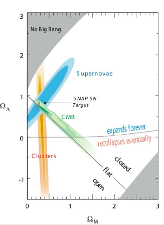
Figure 12: The $(\Omega_{M},\,\Omega_{\Lambda})$ plane with the present data set of cosmological observations $-$ the acceleration of the universe, the large scale structure and the CMB anisotropies $-$ as well as the future determinations by SNAP and Planck of the fundamental parameters which define our Standard Model of Cosmology.

The microwave background has become also a testing ground for theories of particle physics. In particular, it already gives stringent constraints on the mass of the neutrino, when analysed together with large scale structure observations. Assuming a flat $\Lambda$CDM model, the 2-sigma upper bounds on the sum of the masses of light neutrinos is $\sum m_{\nu}<1.0$ eV for degenerate neutrinos (i.e. without a large hierachy between them) if we don’t impose any priors, and it comes down to $\sum m_{\nu}<0.6$ eV if one imposes the bounds coming from the HST measurements of the rate of expansion and the supernova data on the present acceleration of the universe.[28] The final bound on the neutrino density can be expressed as $\Omega_{\nu}\,h^{2}=\sum m_{\nu}/93.2$ eV $\leq 0.01$.

Conclusions

In the last five years we have seen a true revolution in the quality and quantity of cosmological data that has allowed cosmologists to determine most of the cosmological parameters with a few percent accuracy and thus fix a Standard Model of Cosmology. The art of measuring the cosmos has developed so rapidly and efficiently that one may be temped of renaming this science as Cosmonomy, leaving the word Cosmology for the theories of the Early Universe. In summary, we now know that the stuff we are made of $-$ baryons $-$ constitutes just about 4% of all the matter/energy in the Universe, while 25% is dark matter $-$ perhaps a new particle species related to theories beyond the Standard Model of Particle Physics $-$, and the largest fraction, 70%, some form of diffuse tension also known as dark energy $-$ perhaps a cosmological constant. The rest, about 1%, could be in the form of massive neutrinos.

Nowadays, a host of observations $-$ from CMB anisotropies and large scale structure to the age and the acceleration of the universe $-$ all converge towards these values, see Fig. 12. Fortunately, we will have, within this decade, new satellite experiments like Planck, CMBpol, SNAP as well as deep galaxy catalogs from Earth, to complement and precisely pin down the values of the Standard Model cosmological parameters below the percent level, see Table 1.

All these observations would not make any sense without the overall structure of the inflationary paradigm that determines the homogeneous and isotropic background on top of which it imprints an approximately scale invariant gaussian spectrum of adiabatic fluctuations. At present all observations are consistent with the predictions of inflation and hopefully in the near future we may have information, from the polarization anisotropies of the microwave background, about the scale of inflation, and thus about the physics responsible for the early universe dynamics.

References

- [1] A. Einstein, Sitz. Preuss. Akad. Wiss. Phys. 142 (1917) (§4); Ann. Phys. 69 (1922) 436.
- [2] A. Friedmann, Z. Phys. 10 (1922) 377.
- [3] E.P. Hubble, Publ. Nat. Acad. Sci. 15 (1929) 168.
- [4] G. Gamow, Phys. Rev. 70 (1946) 572; Phys. Rev. 74 (1948) 505.
- [5] A.A. Penzias and R.W. Wilson, Astrophys. J. 142 (1965) 419.
- [6] S. Weinberg, Gravitation and Cosmology (John Wiley & Sons, San Francisco, 1972).
- [7] W. L. Freedman et al., Astrophys. J. 553 (2001) 47.
- [8] S. Perlmutter et al. [Supernova Cosmology Project], Astrophys. J. 517 (1999) 565. Home Page http://scp.berkeley.edu/
-
[9]
A. G. Riess et al. [High-z Supernova Search],
Astron. J. 116 (1998) 1009.
Home Page http://cfa-www.harvard.edu/cfa/oir/Research/supernova/ - [10] J. García-Bellido in European School of High Energy Physics, ed. A. Olchevski (CERN report 2000-007); e-print Archive: hep-ph/0004188.
- [11] R. A. Knop et al., e-print Archive: astro-ph/0309368.
- [12] A. G. Riess et al., e-print Archive: astro-ph/0402512.
- [13] The SuperNova/Acceleration Probe Home page: http://snap.lbl.gov/
- [14] F. Zwicky, Helv. Phys. Acata 6 (1933) 110.
- [15] K.C. Freeman, Astrophys. J. 160 (1970) 811.
- [16] C.M. Baugh et al., “Ab initio galaxy formation”, e-print Archive: astro-ph/9907056; Astrophys. J. 498 (1998) 405.
- [17] F. Prada et al., Astrophys. J. 598 (2003) 260.
- [18] C.L. Sarazin, Rev. Mod. Phys. 58 (1986) 1.
- [19] M. Bartelmann et al., Astron. & Astrophys. 330 (1998) 1; M. Bartelmann and P. Schneider, “Weak Gravitational Lensing”, e-print Archive: astro-ph/9912508.
- [20] E.R. Harrison, Phys. Rev. D 1 (1970) 2726; Ya. B. Zel’dovich, Astron. Astrophys. 5 (1970) 84.
- [21] M. Colless et al. [2dFGRS Collaboration], “The 2dF Galaxy Redshift Survey: Final Data Release,” e-print Archive: astro-ph/0306581. The 2dFGRS Home Page: http://www.mso.anu.edu.au/2dFGRS/
- [22] M. Tegmark et al. [SDSS Collaboration], Astrophys. J. 606 (2004) 702; Phys. Rev. D 69 (2004) 103501. The SDSS Home Page: http://www.sdss.org/sdss.html
- [23] R.H. Dicke, P.J.E. Peebles, P.G. Roll and D.T. Wilkinson, Astrophys. J. 142 (1965) 414.
- [24] J.C. Mather et al., Astrophys. J. 512 (1999) 511.
- [25] C.L. Bennett et al., Astrophys. J. 464 (1996) L1.
- [26] D. N. Spergel et al., Astrophys. J. Suppl. 148 (2003) 175; The WMAP Collaboration: http://map.gsfc.nasa.gov/
- [27] D. Scott, J. Silk and M. White, Science 268 (1995) 829; W. Hu, N. Sugiyama and J. Silk, Nature 386 (1997) 37.
- [28] V. Barger, D. Marfatia and A. Tregre, “Neutrino mass limits from SDSS, 2dFGRS and WMAP,” e-print Archive: hep-ph/0312065; P. Crotty, J. Lesgourgues and S. Pastor, “Current cosmological bounds on neutrino masses and relativistic relics,” e-print Archive: hep-ph/0402049.