The Fundamental-Weak Scale Hierarchy in the Standard Model

Abstract

The multiple point principle, according to which several vacuum states with the same energy density exist, is put forward as a fine-tuning mechanism predicting the ratio between the fundamental and electroweak scales in the Standard Model (SM). It is shown that this ratio is exponentially huge: $\sim e^{40}$. Using renormalisation group equations for the SM, we obtain the effective potential in the 2-loop approximation and investigate the existence of its postulated second minimum at the fundamental scale. The investigation of the evolution of the top quark Yukawa coupling constant in the 2-loop approximation shows that, with initial values of the top Yukawa coupling in the interval $h(M_{t})=0.95\pm 0.03$ (here $M_{t}$ is the top quark pole mass), a second minimum of the SM effective potential can exist in the region $\phi_{min2}\approx 10^{16}-10^{22}$ GeV. A prediction is made of the existence of a new bound state of 6 top quarks and 6 anti-top quarks, formed due to Higgs boson exchanges between pairs of quarks/anti-quarks. This bound state is supposed to condense in a new phase of the SM vacuum. This gives rise to the possibility of having a phase transition between vacua with and without such a condensate. The existence of three vacuum states (new, electroweak and fundamental) solves the hierarchy problem in the SM.

¹ E-mail: c.froggatt@physics.gla.ac.uk
² E-mail: laper@heron.itep.ru
³ E-mail: hbech@nbi.dk

1. Introduction: cosmological constant and multiple-point principle

One of the main goals of physics today is to find the fundamental theory beyond the Standard Model (SM). The vast majority of the available experimental information is already explained by the SM. Until now, there is no evidence for the existence of any particles or bound states composed of new particles other than those of the SM. All accelerator physics is in agreement with the SM, except for neutrino oscillations. Presently only this neutrino physics, together with astrophysics and cosmology, gives us any phenomenological evidence for going beyond the SM.

In first approximation one might ignore these indications of new physics and consider the possibility that the SM essentially represents physics well up to the Planck scale. In the present paper, developing the ideas of Ref. [1], we suggest a scenario, using only the pure SM, in which an exponentially huge ratio between the fundamental (Planck) and electroweak scales results:

$$\frac{\mu_{fundamental}}{\mu_{electroweak}}\sim e^{40}.$$

This exponentially huge scale ratio occurs due to the required degeneracy of the three vacuum states discussed in Refs.[2,3].

In such a scenario it is reasonable to assume the existence of a simple and elegant postulate which helps us to explain the SM parameters: couplings, masses and mixing angles. In our model such a postulate is based on a phenomenologically required result in cosmology [4]: the cosmological constant is zero, or approximately zero, meaning that the vacuum energy density is very small. A priori it is quite possible for a quantum field theory to have several minima of its effective potential as a function of its scalar fields. Postulating zero cosmological constant, we are confronted with a question: is the energy density, or cosmological constant, equal to zero (or approximately zero) for all possible vacua or it is zero only for that vacuum in which we live?

This assumption would not be more complicated if we postulate that all the vacua which might exist in Nature, as minima of the effective potential, should have approximately zero cosmological constant. This postulate corresponds to what we call the Multiple Point Principle (MPP) [5,6].

MPP postulates: there are many vacua with the same energy density or cosmological constant, and all cosmological constants are zero or approximately zero.

There are circa 20 parameters in the SM characterizing the couplings and masses of the fundamental particles, whose values can only be understood in speculative models extending the SM. In Ref. [7] it was shown that the Family Replicated Gauge Group (FRGG) model, suggested in Refs. [8,9] as an extension of the SM (see also the reviews [10,11]), fits the SM fermion masses and mixing angles and describes all neutrino experimental data order of magnitudewise using only 5 free parameters – five vacuum expectation values of the Higgs fields which break the FRGG symmetry to the SM. This approach based on the FRGG–model was previously called Anti–Grand Unified Theory (AGUT) and developed as a realistic alternative to SUSY Grand Unified Theories (GUTs)  [12-16]. In Refs. [17,18] the MPP was applied to the investigation of phase transitions in regularized gauge theories. It was shown in [19] that MPP forbids the existence of a fourth generation. A tiny order of magnitude of the cosmological constant was explained in a model involving supersymmetry breaking in N=1 supergravity and MPP [20]. An investigation of the hierarchy problem in the SM extended by MPP and two Higgs doublets is in progress [21].

In the present paper we use MPP with the aim of solving the hierarchy problem, in the sense that we give a crude prediction for the fundamental to electroweak scale ratio in the pure SM. It is necessary to emphasize that this result essentially depends on predicting the value of the top quark Yukawa coupling constant consistent with experiment at the electroweak scale. This prediction entails the existence of a new bound state of 6 top quarks and 6 anti-top quarks, which condenses in a new phase of the SM vacuum  [2,3,7]. In addition we require the existence of a third SM vacuum, with a Higgs field expectation value of the order of the fundamental scale, which we discuss first in terms of the renormalization group improved potential.

2. The renormalization group equation for the effective potential

2.1. The Callan-Symanzik equation

In the theory of a single scalar field interacting with a gauge field, the effective potential $V_{eff}(\phi_{c})$ is a function of the classical field $\phi_{c}$ given by

$$V_{eff}=-\sum_{0}^{\infty}\frac{1}{n!}\Gamma^{(n)}(0)\phi_{c}^{n},$$ (1)

where $\Gamma^{(n)}(0)$ is the one-particle irreducible (1PI) n-point Green’s function calculated at zero external momenta.

The renormalization group equation (RGE) for the effective potential means that the potential cannot depend on a change in the arbitrary renormalization scale parameter M:

$$\frac{dV_{eff}}{dM}=0.$$ (2)

The effects of changing it are absorbed into changes in the coupling constants, masses and fields, giving so-called running quantities.

Considering the renormalization group (RG) improvement of the effective potential [22,23] and choosing the evolution variable as

$$t=\log(\mu/M)=\log(\phi/M),$$ (3)

where $\mu$ is the energy scale, we have the Callan-Symanzik [24,25] RGE for the full $V_{eff}(\phi_{c})$ with $\phi\equiv\phi_{c}$ :

$$(M\frac{\partial}{\partial M}+\beta_{m^{2}}\frac{\partial}{\partial m^{2}}+\beta_{\lambda}\frac{\partial}{\partial\lambda}+\beta_{g}\frac{\partial}{\partial g}+\gamma\,\phi\frac{\partial}{\partial\phi})V_{eff}(\phi)=0,$$ (4)

where M is a renormalization mass scale parameter, $\beta_{m^{2}}$, $\beta_{\lambda}$, $\beta_{g}$ are the RG beta functions for the scalar mass squared $m^{2}$, the scalar field self-interaction $\lambda$ and the gauge couplings respectively. Also $\gamma$ is the anomalous dimension, and the set of gauge coupling constants for the SM are: $g_{i}=(g^{\prime},g,g_{3})$ for the $U(1)_{Y}$, $SU(2)_{L}$ and $SU(3)_{c}$ groups. Here the couplings depend on the renormalization scale M: $\lambda=\lambda(M)$, $m^{2}=m^{2}(M)$ and $g_{i}=g_{i}(M)$. In the following we shall also introduce the top quark Yukawa coupling $h\stackrel{{\scriptstyle def}}{{=}}g_{t}$ and neglect the Yukawa couplings of all the lighter fermions.

It is convenient to introduce a more compact notation for the parameters of the theory. Define:

$$\lambda_{p}=(m^{2},\,\lambda,\,g),$$ (5)

so that the RGE can be abbreviated as

$$(M\frac{\partial}{\partial M}+\beta_{p}\frac{\partial}{\partial\lambda_{p}}+\gamma\,\phi\frac{\partial}{\partial\phi})V_{eff}=0.$$ (6)

The general solution of the above-mentioned RGE has the following form [22]:

$$V_{eff}=-\frac{m^{2}(\phi)}{2}[G(t)\phi]^{2}+\frac{\lambda(\phi)}{8}[G(t)\phi]^{4}+C,$$ (7)

where

$$G(t)=\exp(-\int_{0}^{t}\gamma(t^{\prime})dt^{\prime}).$$ (8)

We shall also use the notation $\lambda(t)=\lambda(\phi)$, $m^{2}(t)=m^{2}(\phi)$, $g_{i}^{2}(t)=g_{i}^{2}(\phi)$, which should not lead to any misunderstanding. In the loop expansion $V_{eff}$ is given by

$$V_{eff}=V^{(0)}+\sum_{n=1}^{\infty}V^{(n)},$$ (9)

where $V^{(0)}$ is the tree-level potential of the SM. Similarly the RG $\beta$-functions have the expansion:

$$\beta_{p}=\sum_{n=1}^{\infty}\beta_{p}^{(n)},\quad\gamma=\sum_{n=1}^{\infty}\gamma^{(n)},$$ (10)

where $X^{(n)}$ is the n-loop contribution to X.

Finally, following Sher’s method [23], we have the following equations for the arbitrary loop approximation:

$$M\frac{\partial}{\partial M}V^{(1)}+D_{1}V^{(0)}=0$$ (11)

- for the one-loop approximation,

$$M\frac{\partial}{\partial M}V^{(2)}+D_{2}V^{(0)}+D_{1}V^{(1)}=0$$ (12)

- for the two-loop approximation,

.

.

.

$$M\frac{\partial}{\partial M}V^{(n)}+D_{n}V^{(0)}+D_{n-1}V^{(1)}+...+D_{1}V^{(n-1)}=0$$ (13)

- for the n-loop approximation. Here the differential operator $D_{k}$ is defined by

$$D_{k}=\beta_{p}^{(k)}\frac{\partial}{\partial\lambda_{p}}-\gamma^{(k)}\phi\frac{\partial}{\partial\phi},\quad k=1,2,3,...$$ (14)

So we have a recursion formula for the calculation of the n-loop contribution to $V_{eff}$, using the tree-level potential and RG functions.

2.2. The tree-level Higgs potential

The Higgs mechanism is the simplest mechanism leading to the spontaneous symmetry breaking of a gauge theory. In the SM the breaking

$$SU(2)_{L}\times U(1)_{Y}\to U(1)_{em},$$ (15)

achieved by the Higgs mechanism, gives masses to the gauge bosons $W^{\pm}$, $Z$, the Higgs boson and the fermions.

With one Higgs doublet of $SU(2)_{L}$, we have the following tree–level Higgs potential:

$$V^{(0)}=-m^{2}\Phi^{+}\Phi+\frac{\lambda}{2}(\Phi^{+}\Phi)^{2}.$$ (16)

The vacuum expectation value of $\Phi$ is:

$$<\Phi>=\frac{1}{\sqrt{2}}\left(\begin{array}[]{c}0\\ {\it v}\end{array}\right),$$ (17)

where

$$v=\sqrt{\frac{2m^{2}}{\lambda}}\approx 246\,\,{\mbox{GeV}}.$$ (18)

Introducing a four-component real Higgs field $\phi$ normalised such that

$$\Phi^{+}\Phi=\frac{1}{2}\phi^{2},$$ (19)

where

$$\phi^{2}=\sum_{i=1}^{4}\phi_{i}^{2},$$ (20)

we have the following tree-level potential:

$$V^{(0)}=-\frac{1}{2}m^{2}\phi^{2}+\frac{1}{8}\lambda\phi^{4}.$$ (21)

As is well-known, the masses of the gauge bosons $W$ and $Z$, a fermion with flavor $f$ and the physical Higgs boson $H$ are expressed in terms of the VEV parameter $v$:

$$M_{W}^{2}=\frac{1}{4}g^{2}v^{2},$$ (22)

$$M_{Z}^{2}=\frac{1}{4}(g^{2}+g^{\prime 2})v^{2},$$ (23)

$$m_{f}=\frac{1}{\sqrt{2}}h_{f}v,$$ (24)

$$M_{H}^{2}=\lambda v^{2},$$ (25)

where $h_{f}$ is the Yukawa coupling for the fermion with flavor $f$.

2.3. The two-loop SM effective potential

In the SM we use RGEs with $\beta$-functions:

$$\beta_{\lambda_{p}}=\frac{d\lambda_{p}}{dt}$$ (26)

given by Ref. [26] in the one-loop and two-loop approximations (see the Appendix).

Using these $\beta$-functions, it is easy to calculate the one–loop effective potential [23]:

$$V_{eff}(1-loop)=-\frac{1}{2}m^{2}\phi^{2}+\frac{\lambda}{8}\phi^{4}+\frac{1}{2}a\phi^{4}\log(\frac{\phi^{2}}{M^{2}})+$$

$$\frac{1}{64\pi^{2}}[(m^{2}-\frac{3}{2}\lambda\phi^{2})^{2}\log(\frac{-m^{2}+\frac{3}{2}\lambda\phi^{2}}{M^{2}})+(m^{2}-\frac{1}{2}\lambda\phi^{2})^{2}\log(\frac{-m^{2}+\frac{1}{2}\lambda\phi^{2}}{M^{2}})]+C,$$ (27)

where C is a constant,

$$a=\frac{1}{32\pi^{2}}(\frac{3}{8}g^{\prime 4}+\frac{3}{4}g^{\prime 2}g^{2}+\frac{9}{8}g^{4}-6h^{4})$$ (28)

and the couplings are evaluated at the renormalization scale M. Here radiative corrections due to the scalar mass term are taken into account.

Following the same procedure [23] of imposing a loop expansion on the RGE of $V_{eff}$ and using all the RGEs [26], we have calculated the 2–loop effective potential in the limit:

$$\phi^{2}>>v^{2},\quad\quad\phi^{2}>>m^{2}.$$ (29)

In general, $V_{eff}$ is given by the following series:

$$V_{eff}\approx V^{(0)}+V^{(1)}+V^{(2)}+...$$ (30)

Neglecting the radiative corrections due to the scalar mass term, we obtain the following expression for $V^{(2)}$:

$$M\frac{\partial}{\partial M}V^{(2)}=-A^{(2)}\phi^{4}-B^{(2)}\phi^{4}\log(\frac{\phi^{2}}{M^{2}}),$$ (31)

where

$$A^{(2)}=\frac{1}{8}\gamma^{(1)}(\beta_{\lambda}^{(1)}+4\lambda\,\gamma^{(1)})+\frac{1}{2}\lambda\,\gamma^{(2)}+\frac{1}{8}\beta_{\lambda}^{(2)},$$ (32)

$$B^{(2)}=\frac{1}{4}\gamma^{(1)}(\beta_{\lambda}^{(1)}+4\lambda\,\gamma^{(1)})+\frac{3}{32\pi^{2}}\lambda\,\beta_{\lambda}^{(1)}+$$

$$\frac{3}{256\pi^{2}}\beta_{g^{\prime}}^{(1)}(g^{\prime 3}+g^{\prime}g^{2})+\frac{3}{256\pi^{2}}\beta_{g}^{(1)}(3g^{3}+g^{\prime 2}g)-\frac{3}{16\pi^{2}}\beta_{h}^{(1)}h^{3}.$$ (33)

Integrating with respect to $M$ and using the normalization condition:

$$V^{(2)}(\phi^{2}=M^{2})=0,$$ (34)

we obtain:

$$V^{(2)}=\frac{1}{2}A^{(2)}\phi^{4}\log(\frac{\phi^{2}}{M^{2}})+\frac{1}{4}B^{(2)}\phi^{4}(\log\frac{\phi^{2}}{M^{2}})^{2}.$$ (35)

Therefore the two–loop effective potential of the SM for

$$\phi^{2}>>m^{2}$$

becomes:

$$V_{eff}(2-loop)=[\frac{\lambda}{8}+\frac{1}{2}A\log(\frac{\phi^{2}}{M^{2}})+\frac{1}{4}B(\log\frac{\phi^{2}}{M^{2}})^{2}]\phi^{4}+C,$$ (36)

where $C$ is “the cosmological constant”,

$$B\equiv B^{(2)},$$

and

$$A=\frac{1}{8}(\beta_{\lambda}^{(1)}+\beta_{\lambda}^{(2)})+\frac{\lambda}{2}(\gamma^{(1)}+\gamma^{(2)}+(\gamma^{(1)})^{2})+\frac{1}{8}\gamma^{(1)}\beta_{\lambda}^{(1)}.$$ (37)

In terms of the evolution variable $t$ (3), we have:

$$V_{eff}(2-loop)=(\frac{\lambda}{8}+At+Bt^{2})\phi^{4}+C.$$ (38)

3. The second minimum of the effective potential

In this section our goal is to show the possible existence of a second (non-standard) minimum of the effective potential in the pure SM at the fundamental scale:

$$\phi_{min2}>>v=\phi_{min1}.$$ (39)

The tree–level Higgs potential with the standard “weak scale minimum” at $\phi_{min1}=v$ is given by:

$$V(tree-level)=\frac{\lambda}{8}(\phi^{2}-v^{2})^{2}+C.$$ (40)

In accord with cosmological results, we take the cosmological constants $C$ for both vacua equal to zero (or approximately zero): $C=0$ (or $C\approx 0$). The following requirements must be satisfied in order that the SM effective potential should have two degenerate minima:

$$V_{eff}(\phi_{min1}^{2})=V_{eff}(\phi_{min2}^{2})=0,$$ (41)

$$V^{\prime}_{eff}(\phi_{min1}^{2})=V^{\prime}_{eff}(\phi_{min2}^{2})=0,$$ (42)

where

$$V^{\prime}(\phi^{2})=\frac{\partial V}{\partial\phi^{2}}.$$ (43)

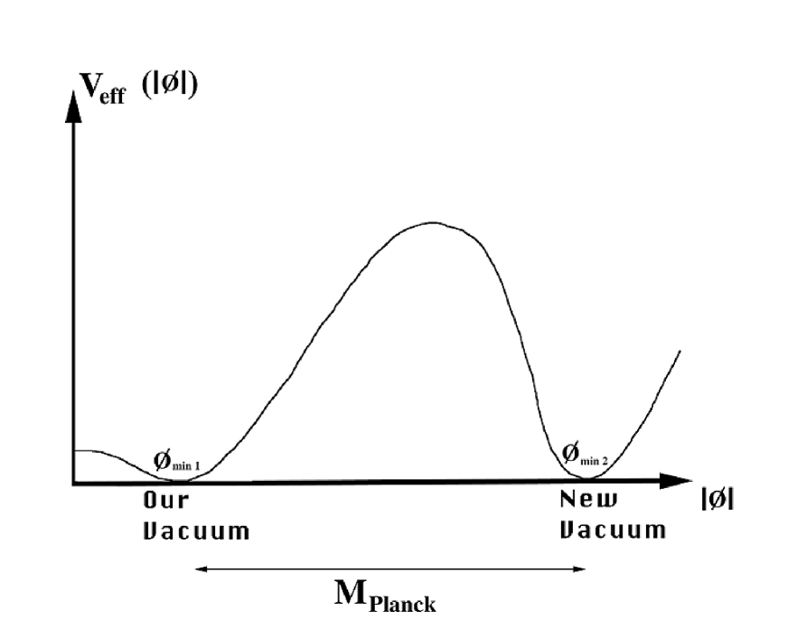
Figure 1: The first (our) vacuum at $|\phi|\approx 246$ GeV and the second vacuum at the fundamental scale $|\phi|\sim M_{Pl}.$

These degeneracy conditions first considered in Ref. [1] correspond to the MPP expectation. The first minimum is the standard “Weak scale minimum”, and the second one is the non-standard “Fundamental scale minimum” (if it exists). An illustrative schematic picture of $V_{eff}$ is presented in Fig. 1.

Here we consider the SM theory with zero temperature ($T=0$). As was shown in Ref. [1], the above MPP-requirements lead to the condition that our electroweak vacuum is barely stable at $T=0$, so that in the pure SM the top quark and Higgs masses should lie on the SM vacuum stability curve, investigated in Refs. [27,28].

With good accuracy, the predictions of Ref. [1] for the top quark and Higgs masses from the MPP requirement of a second degenerate vacuum, together with the identification of its position with the Planck scale $\phi_{min2}=M_{Planck}$, were as follows:

$$M_{t}=173\pm 5\,\,{\mbox{GeV}},\quad M_{H}=135\pm 9\,\,{\mbox{GeV}}.$$ (44)

Later, in Ref. [29], an alternative metastability requirement for the electroweak (first) vacuum was considered, which gave a Higgs mass prediction of $122\pm 11\,\,$ GeV, close to the LEP lower bound of 115 GeV (Particle Data Group [30]).

Following Ref. [1], let us now investigate the conditions, Eqs. (41,42), for the existence of a second degenerate vacuum at the fundamental scale:

$$\phi_{min2}\sim{\mu}_{fundamental}.$$ (45)

For large values of the Higgs field,

$$\phi^{2}>>m^{2},$$ (46)

$V_{eff}$ is very well approximated by the quartic term in Eq. (7) and the degeneracy condition (41) gives:

$$\lambda(\phi_{min2})=0,$$ (47)

The condition (42) for a turning value then gives:

$$\lambda^{\prime}(\phi_{min2})=0$$ (48)

which can be expressed in the form:

$$\beta_{\lambda}(\phi_{min2},\lambda=0)=0.$$ (49)

In the next section we search for the scale $\phi_{min2}$ given by the degeneracy conditions (47,49).

4. The top quark Yukawa coupling constant evolution

The position of the second minimum of $V_{eff}$ essentially depends on the running of the gauge couplings and of the top quark Yukawa coupling. Let us consider first the running of the gauge couplings $g^{\prime},\,g,\,g_{3}$ in accord with the present experimental data.

Starting from the Particle Data Group [30], we have the masses:

$$M_{t}=174.3\pm 5.1\,\,{\mbox{GeV}},$$ (50)

$$M_{Z}=91.1872\pm 0.0021\,{\mbox{GeV}}.$$ (51)

Also for the inverse electromagnetic fine structure constant in the $\overline{MS}$-scheme we have:

$${\hat{\alpha}}^{-1}(M_{Z})=127.93\pm 0.027,$$ (52)

while for the square of the sine of the weak angle in the $\overline{MS}$-scheme we have:

$${\hat{s}}^{2}(M_{Z})=0.23117\pm 0.00016,$$ (53)

and for the QCD fine structure constant we have:

$$\alpha_{3}(M_{Z})=0.117\pm 0.002.$$ (54)

The running top quark mass was considered in Refs. [1,28] and [31-33], for which we have the following value from Eq. (50):

$$m_{t}(M_{t})\approx(165\pm 5)\,\,{\mbox{GeV}},$$ (55)

which is related to the running top quark Yukawa coupling $h(\mu)$ as follows:

$$m_{t}(M_{t})\approx h(M_{t})\frac{v}{\sqrt{2}},$$ (56)

that is:

$$h(M_{t})\approx 0.95\pm 0.03.$$ (57)

It is well-known that, for $\mu>M_{Z}$, the running of all the gauge coupling constants in the SM is well described by the one-loop approximation. So, for $\mu>M_{t}$, we can write:

$$\alpha_{i}^{-1}(\mu)=\alpha_{i}^{-1}(M_{t})+\frac{b_{i}}{2\pi}\log\left(\frac{\mu}{M_{t}}\right),$$ (58)

where

$$\alpha_{Y}=\frac{g^{\prime 2}}{4\pi},\quad\alpha_{2}=\frac{g^{2}}{4\pi},\quad\alpha_{3}=\frac{g_{3}^{2}}{4\pi}$$

i=Y,2,3 for the $U(1)_{Y}$, $SU(2)$ and $SU(3)$ groups, and

$$b_{Y}=-\frac{41}{6},\quad b_{2}=\frac{19}{6},\quad b_{3}=7.$$ (59)

Assuming that this running is valid up to the “fundamental” scale, where new physics enters, we have the following evolutions, which are revised in comparison with Ref. [34] using updated experimental results [30]:

$$\alpha_{Y}^{-1}(t)=97.40\pm 0.04-\frac{41}{12\pi}t,$$ (60)

$$\alpha_{2}^{-1}(t)=29.95\pm 0.02+\frac{19}{12\pi}t,$$ (61)

$$\alpha_{3}^{-1}(t)=9.336\pm 0.170+\frac{7}{2\pi}t.$$ (62)

where

$$t=\log\left(\frac{\mu}{M_{t}}\right)$$ (63)

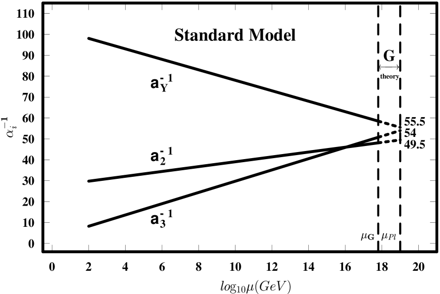
Figure 2: The evolution of the inverse SM fine structure constants $\mbox{a}_{Y,2,3}^{-1}\equiv\alpha_{Y,2,3}^{-1}$ as functions of x ($\mu=10^{x}$ GeV) up to the scale $\mu_{G}\sim M_{Pl}$ where new physics (“G-theory”) enters.

These gauge coupling constant evolutions are given in Fig. 2, where $x=\log_{10}\mu\,(GeV)$.

Now we are ready to solve the RGE for the top quark Yukawa coupling, assuming that it is described by the 1–loop approximation with good accuracy. Taking into consideration the Ford-Jones-Stephenson-Einhorn RGE for h(t) [26], we obtain the following differential equation for $y=\alpha_{h}^{-1}(t)=4\pi/h^{2}(t)$ in the 1-loop approximation:

$$\frac{dy}{dt}=-\frac{9}{4\pi}+F(t)y(t),$$ (64)

where

$$F(t)=\frac{1}{\pi}\left[\frac{17}{24\alpha_{Y}^{-1}(t)}+\frac{9}{8\alpha_{2}^{-1}(t)}+\frac{4}{\alpha_{3}^{-1}(t)}\right].$$ (65)

Now, using the central values of $\alpha_{i}^{-1}(M_{t})$, we can solve the RGE for $y=\alpha_{h}^{-1}(t)$. We take the spread of experimental values of $h(M_{t})$ in Eq. (57) to give us the following choice of initial values:

$$y(M_{t})=\alpha_{h}^{-1}(M_{t})=13.92,\,14.85,\,13.08.$$ (66)

The corresponding solutions for $y(t)$ are presented in Fig. 3 as the bunches of curves 1, 2 and 3 respectively. Each bunch describes the spread in the evolution of $y(t)$ due to the uncertainty in $\alpha_{3}^{-1}(M_{t})$ coming from Eq.(54):

$$\alpha_{3}^{-1}(M_{t})=9.336\pm 0.170.$$ (67)

The influence of the uncertainties in $\alpha_{1,2}(M_{t})$ is negligible.

The curve y1 of Fig. 3 describes the solution for $y=\alpha_{h}^{-1}(t)$ given by the requirement $\beta_{\lambda}(t,\lambda(t)=0)=0$ for a second degenerate minimum. From Eq. (101) in the Appendix, the curve y1 is given by the equation:

$$y_{1}(t)=\left[\frac{1}{16\alpha_{Y}^{-2}(t)}+\frac{1}{8\alpha_{Y}^{-1}(t)\alpha_{2}^{-1}(t)}+\frac{3}{16\alpha_{2}^{-2}(t)}\right]^{-\frac{1}{2}},$$ (68)

in the 1-loop approximation. We note that numerically $y_{1}(t)$ varies rather weakly as a function of $t$, corresponding to a value for the top quark Yukawa coupling of

$$h(\mu_{fundamental})=h(\phi_{min2})\simeq 0.4$$ (69)

at the second or fundamental scale minimum [2,7]. The intersections of this curve y1 with the possible evolutions of $y=\alpha_{h}^{-1}(t)$ in Fig. 3 determine the positions of the second minimum, according to the MPP assumption. In this way we obtain the following positions for the second minimum (at $\mu_{0}=\phi_{min2}$ and $t_{0}=\log(\mu_{0}/M_{t})$), which depend on the value of $h(M_{t})$:

I) $\alpha_{3}(M_{Z})=0.117;$

$$y(M_{t})=13.92,\quad h(M_{t})\approx 0.95,\quad t_{0}\approx 44.5,\quad\mu_{0}\sim 10^{21.5}\,\,\mbox{GeV};$$

$$y(M_{t})=14.85,\quad h(M_{t})\approx 0.92,\quad t_{0}\approx 38.8,\quad\mu_{0}\sim 10^{19}\,\,\mbox{GeV};$$

$$y(M_{t})=13.08,\quad h(M_{t})\approx 0.98,\quad t_{0}\approx 50.7,\quad\mu_{0}\sim 10^{24}\,\,\mbox{GeV};$$

giving the range

$$\phi_{min2}\sim 10^{19}-10^{24}\ \mbox{GeV}.$$

II) $\alpha_{3}(M_{Z})=0.115;$

$$y(M_{t})=13.92,\quad h(M_{t})\approx 0.95,\quad t_{0}\approx 42,\quad\mu_{0}\sim 10^{20.5}\,\,\mbox{GeV};$$

$$y(M_{t})=14.85,\quad h(M_{t})\approx 0.92,\quad t_{0}\approx 38.3,\quad\mu_{0}\sim 10^{19}\,\,\mbox{GeV};$$

$$y(M_{t})=13.08,\quad h(M_{t})\approx 0.98,\quad t_{0}\approx 50,\quad\mu_{0}\sim 10^{24}\,\,\mbox{GeV};$$

giving the range

$$\phi_{min2}\sim 10^{19}-10^{24}\ \mbox{GeV}.$$

III) $\alpha_{3}(M_{Z})=0.119;$

$$y(M_{t})=13.92,\quad h(M_{t})\approx 0.95,\quad t_{0}\approx 46.3,\quad\mu_{0}\sim 10^{22}\,\,\mbox{GeV};$$

$$y(M_{t})=14.85,\quad h(M_{t})\approx 0.92,\quad t_{0}\approx 40.6,\quad\mu_{0}\sim 10^{20}\,\,\mbox{GeV};$$

$$y(M_{t})=13.08,\quad h(M_{t})\approx 0.98,\quad t_{0}\approx 52.2,\quad\mu_{0}\sim 10^{25}\,\,\mbox{GeV};$$

giving the range

$$\phi_{min2}\sim 10^{20}-10^{25}\ \mbox{GeV}.$$

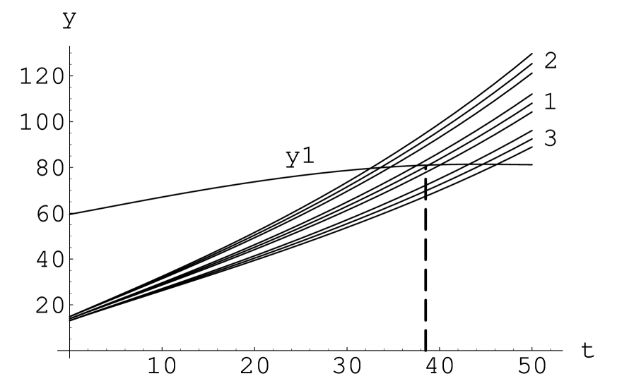
Figure 4: The 2–loop approximation for the evolution of $y(t)=\alpha_{h}^{-1}(t)=4\pi/h^{2}(t)$, where h is the top quark Yukawa coupling constant. Three bunches 1(middle), 2(up), 3(down) of curves correspond respectively to the three values of $h(M_{t})=0.95,\,0.92,\,0.98$ given by experiment. The spread of each bunch corresponds to the experimental values of $\alpha_{3}(M_{Z})=0.117\pm 0.002$ (upper and lower curves correspond to $\alpha_{3}(M_{Z})=0.115$ and $\alpha_{3}(M_{Z})=0.119$ respectively). The curve y1 for $y_{1}$, given by the MPP requirement $\beta_{\lambda}(\lambda=0)=0$, intersects the bunches at points corresponding to the position of the second minimum identified with the fundamental scale in the SM.

We have also calculated the position of the second minimum numerically in the 2-loop approximation. The positions obtained are given in Fig. 4, which correspond to the following values:

I) $\alpha_{3}(M_{Z})=0.117;$

$$y(M_{t})=13.92,\quad h(M_{t})\approx 0.95,\quad t_{0}\approx 38.5,\quad\mu_{0}\sim 10^{19}\,\,\mbox{GeV};$$

$$y(M_{t})=14.85,\quad h(M_{t})\approx 0.92,\quad t_{0}\approx 33,\quad\mu_{0}\sim 10^{17}\,\,\mbox{GeV};$$

$$y(M_{t})=13.08,\quad h(M_{t})\approx 0.98,\quad t_{0}\approx 44,\quad\mu_{0}\sim 10^{21}\,\,\mbox{GeV};$$

giving the range

$$\phi_{min2}\sim 10^{17}-10^{21}\ \mbox{GeV}.$$

II) $\alpha_{3}(M_{Z})=0.115;$

$$y(M_{t})=13.92,\quad h(M_{t})\approx 0.95,\quad t_{0}\approx 36.5,\quad\mu_{0}\sim 10^{18}\,\,\mbox{GeV};$$

$$y(M_{t})=14.85,\quad h(M_{t})\approx 0.92,\quad t_{0}\approx 32,\quad\mu_{0}\sim 10^{16}\,\,\mbox{GeV};$$

$$y(M_{t})=13.08,\quad h(M_{t})\approx 0.98,\quad t_{0}\approx 42,\quad\mu_{0}\sim 10^{20}\,\,\mbox{GeV};$$

giving the range

$$\phi_{min2}\sim 10^{16}-10^{20}\ \mbox{GeV}.$$

III) $\alpha_{3}(M_{Z})=0.119;$

$$y(M_{t})=13.92,\quad h(M_{t})\approx 0.95,\quad t_{0}\approx 39,\quad\mu_{0}\sim 10^{19.5}\,\,\mbox{GeV};$$

$$y(M_{t})=14.85,\quad h(M_{t})\approx 0.92,\quad t_{0}\approx 34,\quad\mu_{0}\sim 10^{17}\,\,\mbox{GeV};$$

$$y(M_{t})=13.08,\quad h(M_{t})\approx 0.98,\quad t_{0}\approx 45.5,\quad\mu_{0}\sim 10^{22}\,\,\mbox{GeV};$$

giving the range

$$\phi_{min2}\sim 10^{17}-10^{22}\ \mbox{GeV}.$$

Thus, the curve y1 of Fig. 4 shows that, in the 2-loop approximation, the experimental values of the coupling constants allow the SM effective potential to have a second minimum in the interval:

$$\phi_{min2}\in(10^{16},10^{22})\,{\mbox{GeV}}.$$ (70)

Here we emphasize that, for the central values of the experimental parameters:

$$\alpha_{s}(M_{Z})\approx 0.117\quad\quad{\mbox{and}}\quad\quad h(M_{t})\approx 0.95,$$

and identifying the position of the second minimum with the fundamental scale, $\mu_{fundamental}=\phi_{min2}$, we predict the fundamental scale to be close to the Planck scale

$$\mu_{fundamental}\sim 10^{19}\,\,{\mbox{GeV}},$$

which coincides with the result of Refs. [1,28,31,32]. We note that for the value $h(M_{t})=0.98$, and for the values $h(M_{t})=0.95$ and $\alpha_{3}(M_{Z})=0.119$, the second minimum of the effective potential turns out to be beyond the Planck scale ($M_{Planck}\sim 10^{19}$ GeV). On the other hand, for the extreme values $\alpha_{s}\approx 0.115$ and $h(M_{t})\approx 0.92$, the fundamental scale becomes $\mu_{fundamental}\approx 10^{16}$ GeV, corresponding to the string scale.

5. The second derivative of the SM effective potential and the second minimum at $10^{19}$ GeV

Let us consider now the second minimum of $V_{eff}$ for the central values of the experimental parameters, when $\phi_{min2}=10^{19}$ GeV or $t_{0}\approx 38.5$. Choosing the renormalization point at $M=\phi_{min2}$, we introduce the following evolution parameter:

$$t^{\prime}=\log(\frac{\phi}{\phi_{min2}}).$$ (71)

With the definition:

$$V\stackrel{{\scriptstyle def}}{{=}}\frac{(16\pi)^{4}}{24}(\phi_{min2}^{-4})V_{eff},$$ (72)

we have obtained the following expression for the effective potential in the two-loop approximation:

$$V=(C_{1}t^{\prime}+C_{2}t^{\prime 2})(\frac{\phi}{\phi_{min2}})^{4}=(C_{1}t^{\prime}+C_{2}t^{\prime 2})e^{4t^{\prime}},$$ (73)

where our calculations gave:

$$C_{1}=(g^{\prime 2}+3g^{2}-4h^{2})(\frac{3}{4}g^{\prime 4}+\frac{3}{2}g^{\prime 2}g^{2}+\frac{9}{4}g^{4}-12h^{4}),$$ (74)

$$C_{2}=2C_{1}+\frac{41}{3}(g^{\prime 6}+g^{\prime 4}g^{2})-\frac{19}{3}(3g^{6}+g^{\prime 2}g^{4})$$

$$-32h^{4}(\frac{9}{2}h^{2}-8g_{3}^{2}-\frac{9}{4}g^{2}-\frac{17}{2}g^{\prime 2}).$$ (75)

Calculating all the parameters at $t_{0}\approx 38.5$, we have:

$$g^{\prime 2}(t_{0})\approx 0.2263,\quad\quad g^{2}(t_{0})\approx 0.2546,\quad\quad g_{3}^{2}(t_{0})\approx 0.2406,\quad\quad h^{2}(t_{0})\approx 0.1571,$$ (76)

and

$$C_{1}\approx-0.00921,\quad\quad C_{2}\approx 2.8639.$$ (77)

5.1. Hierarchy without use of the new bound state?

As emphasized in the introduction, our present explanation for the hierarchy of scales depends crucially on the existence of a third SM phase associated with the condensation of a proposed new bound state. However, we first consider here a superficially appealing argument for the huge scale ratio based just on the existence of two minima in the effective potential and some form of “naturalness”.

Therefore let us consider the second derivative of the effective potential, which has to change its sign from “+” to “-” and back again to “+” in the region between the two minima. We take, as our “naturalness” assumption, that in a polynomial approximation to the second derivative of the effective potential

$$V^{\prime\prime}(t)=\frac{\partial^{2}V}{\partial(\phi^{2})^{2}}=a_{0}+a_{1}t+a_{2}t^{2},$$ (78)

where

$$t=\log(\phi/M_{t})=t^{\prime}+t_{0}\approx t^{\prime}+38.5,$$ (79)

the coefficients can be considered to be random numbers, but with their phenomenological orders of magnitude imposed. In the 0-loop approximation only $a_{0}$ would be different from zero, in the 1-loop approximation only $a_{0}$ and $a_{1}$ would be non-zero and so on. In fact the ratios of successive expansion coefficients $r_{1}=|a_{1}/a_{0}|$, $r_{2}=|a_{2}/a_{1}|$,… are expected to be of the order of magnitude $\beta_{\lambda_{p}}/\lambda_{p}$. This expectation expresses the idea that the variation of $V^{\prime\prime}$, which in first approximation is proportional to $\lambda(\phi)=\lambda(t)$, is given by the beta functions $\beta_{\lambda_{p}}$ of Eq. (26) measured relative to the respective couplings $\lambda_{p}$. Phenomenological values for these relative rates of variation $\beta_{\lambda_{p}}/\lambda_{p}$, evaluated at the Planck scale say, are typically numbers of the order of 1/90.

We may check this idea by evaluating the expansion coefficient ratios $r_{1}$ and $r_{2}$ for our expansion Eq. (78), using Eqs. (73,77). Indeed we find the coefficients $a_{i}$ to be

$$a_{0}\approx 8161.2,\quad a_{1}\approx-432.46,\quad a_{2}\approx 5.7277,$$ (80)

which give the ratios:

$$r_{1}=|\frac{a_{1}}{a_{0}}|\approx 0.0529\sim\frac{1}{19},\quad\quad r_{2}=|\frac{a_{2}}{a_{1}}|\approx 0.0132\sim\frac{1}{75}.$$ (81)

So we see that these expansion ratios are indeed small, of the order 1/19 to 1/75; not so very different from the suggested 1/90.

With random coefficients having ratios of this order of magnitude, we would expect the typical range in $t$ with $V^{\prime\prime}<0$ between two regions with $V^{\prime\prime}>0$, for a second derivative $V^{\prime\prime}$ having such an expansion, should have a length $\Delta t$ of order 19 to 75, or say 90. Consequently there should be a similar range $\Delta t$ between the first and second minimum of $V$, implying an exponentially huge scale ratio of the order:

$$\frac{\phi_{min2}}{\phi_{min1}}\sim\exp(\Delta t)\sim\exp(19\ \mbox{to}\ 75\ \mbox{or}\ 90)$$ (82)

In this way we seem to have solved the huge scale ratio problem – here taken to be the ratio of the Higgs field values in the two assumed minima of the effective potential.

However we must immediately admit that this solution is not satisfactory! Imposing the phenomenologically needed small Higgs mass of order $\phi_{min1}$, the quartic $\phi^{4}$ term comes to dominate the Higgs effective potential in most of the region between the two minima and near $\phi_{min2}$. So then $V^{\prime\prime}(t)$ roughly functions as the running self-coupling $\lambda(t)$. But now, generically in the above scenario, $V^{\prime\prime}(t)$ is negative in a large interval, which would cause the effective potential $V_{eff}$ to be negative and make our vacuum severely unstable.

Contrary to this general expectation, our data-based picture with the degenerate vacuum conditions, Eqs. (47,48), imposed is fine-tuned in such a way as to avoid this problem of negative values for the effective potential. It can indeed be readily seen that the coefficients $a_{i}$ of Eq. (95) are not random, which would require the distance $\Delta t$ between the zeros of $V^{\prime\prime}$ to be of the order of 19 to 75 or 90. However, as one sees from Fig. 5, in our realistic picture the two zeros of $V^{\prime\prime}$ are only about one unit in $t$ apart! This behavior of $V^{\prime\prime}(t^{\prime})$ was determined using the following expansion:

$$V^{\prime\prime}=at^{\prime 2}+bt^{\prime}+c,$$ (83)

where from Eq. (73)

$$a=2C_{2},\quad b=2C_{1}+3C_{2},\quad c=\frac{3C_{1}+C_{2}}{2},$$ (84)

and from Eq. (77)

$$a\approx 5.7277,\quad b\approx 8.5731,\quad c\approx 1.4181.$$ (85)

It is a parabola with the above-mentioned sign changes, having zeros at the following positions:

$$t^{\prime}_{1}=-1.3074,\quad t^{\prime}_{2}=-0.1894,$$ (86)

and

$${\mbox{min}}\,V^{\prime\prime}=-1.7899.$$ (87)

The shape of the second minimum at $\phi_{min2}=10^{19}$ GeV is presented in Fig. 6 for V given by Eq. (72).

Near the minimum of V at $10^{19}$ GeV, the Higgs self-coupling $\lambda(t^{\prime})$ is well described by the expression:

$$\lambda(t^{\prime})G^{4}(t^{\prime})=\frac{192}{(16\pi)^{4}}(C_{1}t^{\prime}+C_{2}t^{\prime 2}).$$ (88)

The behavior of $\lambda(t^{\prime})$ near the second minimum is shown in Fig. 7 for different values of $h(M_{t})$. The behavior of $\lambda(t)$ at lower energies was obtained and shown in Refs. [1,35].

In concluding this part of our paper, we should emphasize that the MPP-description of the SM predicts a value for the Higgs mass. In spite of the large uncertainty in the position of the second minimum, the value of $\lambda$ at the electroweak scale is predicted to lie in the narrow interval:

$$\lambda(M_{t})\in(0.27;\,0.34),$$ (89)

which corresponds to the prediction of the Higgs mass given in Ref. [1]: $M_{H}\approx 135\pm 9$ GeV. In this scenario new physics enters at a scale of the order of $10^{19}$ GeV.

6. A new bound state in the SM

The MPP helps to solve fine-tuning problems; in particular the hierarchy problem of why the electroweak scale is so tiny in comparison with the Planck scale.

It is well-known that, when calculating the square of the SM Higgs mass, we have to deal with the quadratic divergencies which occur order by order in the perturbative expansion. The bare Higgs mass squared needs to be fine-tuned in all orders of this perturbation series. Near the (cut-off) Planck scale these quadratic divergencies become $(\Lambda_{Planck}/\Lambda_{weak})^{2}$ (that is, $(10^{17})^{2}=10^{34}$) times bigger than the final Higgs mass squared, and it is clear that a fine-tuning by 34 digits is needed to solve the hierarchy problem in the SM. Supersymmetry can remove these divergencies by having a cancellation between fermion and boson contributions. Hence supersymmetry solves the technical hierarchy problem. But the problem still exists in the form of why the soft supersymmetry breaking terms are small compared to the fundamental Planck scale.

At first sight, it seems difficult to explain the cancellation of such divergencies by the MPP protected fine-tuning. The energy density, or cosmological constant, has the dimension of energy to the fourth power, so that modes with Planck scale frequencies contribute $(10^{17})^{4}=10^{68}$ times more than those at the electroweak scale. Nevertheless, we can obtain such a fine-tuning by assuming the existence of two degenerate phases in the SM which are identical for the highest modes, but deviate by their physics at the electroweak scale. Thus the way to solve the hierarchy problem in the SM using MPP is to consider a new phase at the electroweak scale, different from and degenerate with the Weinberg-Salam Higgs phase. The obvious way to achieve this is to find a scalar bound state $\phi_{bound}$ made out of SM particles, which is so strongly bound that it becomes tachyonic and condenses into the vacuum. Of course we do not expect that the tachyons should really exist in Nature, but that the vacuum condensate should adjust itself to such a density as to bring the mass squared of the bound state back to be positive. As was shown in Refs. [2,3,7], an attractive candidate for such a bound state could be composed from $6t+6\bar{t}$ quarks.

Here the Weinberg-Salam Higgs particle exchange plays an essential part. The virtual exchange of Higgs scalar bosons between $qq$, $q\bar{q}$ and $\bar{q}\bar{q}$ yields an attractive force in all cases. The bound state of a top quark and an anti-top quark (toponium) is mainly bound by gluon exchange, although Higgs exchange is comparable. But if we add more top or anti-top quarks, then the Higgs exchange continues to attract while the gluon exchange saturates and gets less significant. The maximal binding energy per particle comes from the S-wave $6t+6\bar{t}$ ground state. The reason is that the $t$ quark has 2 spin states and 3 colour states. This means that, by the Pauli principle, only $2\times 3=6\ t$ quarks can be put in an S-wave function, together with $6\ \bar{t}$-quarks. So, in total, we have 12 $t$ quark/anti-quark constituents together in relative S-waves. If we try to put more $t$ and $\bar{t}$ quarks together, then some of them will go into a P-wave for which the pair binding energy will decrease by at least a factor of 4.

Estimating the pair binding energy using the Bohr formula for atomic energy levels (here for each quark, we treat the remaining 11 quarks as a nucleus), the authors of Refs. [2,7] have obtained an approximate expression for the mass squared of the $6t+6\bar{t}$ bound state. Their result for the mass squared of the bound state, crudely estimated from the non-relativistic binding energy, is:

$$m_{bound}^{2}=(12m_{t})^{2}-2(12m_{t})\times E_{binding}+...\approx(12m_{t})^{2}(1-\frac{33}{8\pi^{2}}h^{4}+...),$$ (90)

The condition that this bound state should be tachyonic leads to the requirement:

$$(1-\frac{33}{8\pi^{2}}h^{4}+....)\leq 0.$$ (91)

When the bound state becomes tachyonic, we should be in a vacuum state with

$$<\phi_{bound}>\neq 0.$$ (92)

Hence we expect a phase transition to the new phase at the point where the bound state mass squared passes zero as a function of the top quark Yukawa coupling $h$:

$$m^{2}_{bound}=0,$$ (93)

According to Refs. [2,3,7], this condition gives:

$$h_{p.t.}\approx\sqrt{\pi\sqrt{\frac{8}{33}}}\approx 1.24,$$ (94)

where “p.t.” means the value at the “phase transition”.

Taking into account a possible correction due to the Higgs field quantum fluctuations, we gave the following estimate in Ref. [3]:

$$h_{p.t.}(\mu_{electroweak})=1.06\pm 0.18,$$ (95)

which is in agreement with the experimental value of the top quark Yukawa coupling constant at the electroweak scale: $h_{exper}(M_{t})=0.95\pm 0.03$. It seems that we have a successful confirmation of the MPP hypothesis based on pure SM physics at the electroweak scale. In principle a more accurate (but hard) SM calculation of the top quark Yukawa coupling at the phase transition, $h_{p.t.}$, would provide a very clean test of MPP.

Now we have not two, but three vacua in the SM with the same energy density and in the next section we explain how they lead to a resolution of the hierarchy problem in the SM.

7. The hierarchy of scales in the SM

Requiring the same energy density of three SM vacua (new, standard and fundamental), we have obtained predictions for the running top quark Yukawa coupling $h(t)$ at the fundamental scale $\mu_{fundamental}$, Eq. (69), and the electroweak scale $\mu_{electroweak}$, Eq. (95). So we can now use the RGE for the top quark Yukawa coupling to estimate the ratio of the fundamental and electroweak scales needed to generate the required amount of renormalization group running of $h(t)$. It is assumed here that we can take the values of the SM fine structure constants at the fundamental scale, $\alpha_{i}(\mu_{fundamental})$, as given and, in particular, we take $\alpha_{3}(\mu_{fundamental})\simeq 1/54$ (see Fig. 2). Due to the relative smallness of the beta function $\beta_{h}(\mu_{fundamental})$ at the fundamental scale, we need many $e$-foldings between $\mu_{fundamental}$ and $\mu_{electroweak}$. For definiteness, let us assume that the MPP prediction, Eq. (95), is correct and coincides with the experimental value $h(\mu_{electroweak})\simeq 0.95$. Then we can use the results of section 4 to give the MPP prediction for the ratio between the fundamental and electroweak scales:

$$\frac{\mu_{fundamental}}{\mu_{electroweak}}\sim 10^{17}\sim e^{40}.$$ (96)

This exponentially huge scale ratio provides our MPP solution to the hierarchy problem in the SM. In the scenario developed in this paper we essentially have a “great desert” between the electroweak and fundamental scales: no new physics, with the exception perhaps of neutrinos at the see-saw scale.

8. Conclusions

As a way of predicting the ratio of the fundamental (Planck) scale to the electroweak scale, we have developed the idea of the Multiple Point Principle which states that there exist several different vacuum states in Nature having the same energy density; more precisely, all vacua having approximately zero energy density or cosmological constant.

Neglecting mass terms, we have used the RGE for the SM effective potential and obtained an explicit expression for this effective potential in the two-loop approximation for large values of the Weinberg-Salam Higgs scalar field: $\phi^{2}>>m^{2}$.

We have considered the running of the gauge and top quark Yukawa couplings, investigating the conditions for the existence of a second minimum of the effective potential in the pure SM. Our investigation of the evolution of the top quark Yukawa coupling constant showed that the experimentally established value at the electroweak scale, $h(M_{t})=0.95\pm 0.03$, is consistent with a second minimum of the SM effective potential existing in the interval:

$$\phi_{min2}\in(10^{16},10^{22})\ {\mbox{GeV}.}$$

The central experimental values $h(M_{t})=0.95$ and $\alpha_{3}(M_{Z})=0.117$, together with the vacuum degeneracy conditions (47,49), predict a second minimum at $\phi_{min2}\approx 10^{19}$ GeV. We presented the shape of this second minimum, showing the sign changes of the second derivative of the SM effective potential in the region $\mu\leq\phi_{min2}$.

In the framework of the MPP solution of the hierarchy problem, we have investigated the possible existence of a very strongly bound state of 6 top quarks and 6 anti-top quarks due, in the main, to Weinberg-Salam Higgs boson exchanges between pairs of quarks/anti-quarks. This $6t+6\bar{t}$ bound state is supposed to condense in a new phase of the SM vacuum, for which $<\phi_{bound}>\sim\mu_{electroweak}$. An estimate of the top quark Yukawa coupling $h_{p.t.}$ at the critical point of the phase transition between the “new” phase and the “weak” phase revealed that MPP may explain why $h(M_{t})\approx 1$, in accord with experiment.

We have shown that the requirement of the degeneracy of the three vacua (new, weak and fundamental) leads to the prediction of an exponentially huge scale ratio:

$$\frac{\mu_{fundamental}}{\mu_{electroweak}}\sim e^{40},$$

in the absence of new physics between the electroweak and fundamental scales (with the exception of neutrinos).

9. Acknowledgements

This work was supported by the Russian Foundation for Basic Research (RFBR), project No.02-02-17379. L.V.L. and H.B.N. thank R.Barbieri and the directors of the Conference on Hierarchy Problems in Four and More Dimensions (Italy, Trieste, 1-4 October, 2003) for the wonderful organization of the Conference and useful discussion of the talk based on this investigation. L.V.L. thanks all participants at her Niels Bohr Institute theoretical seminar, especially P.H.Damgaard, D.Diakonov, N.Obers and F.Sannino, for fruitful discussions and comments. We also thank our colleagues D.L.Bennett and R.B.Nevzorov for their helpful discussions and advice.

10. Appendix

In this Appendix we give the results of Ref. [26] for the RGE $\beta$-functions in the one-loop and two-loop approximations.

The one-loop beta-functions in the SM are:

$$16\pi^{2}\beta_{g^{\prime}}^{(1)}=(\frac{10}{9}N_{f}+\frac{1}{6}N_{S})g^{\prime 3},$$ (97)

$$16\pi^{2}\beta_{g}^{(1)}=(\frac{2}{3}N_{f}+\frac{1}{6}N_{S}-\frac{22}{3})g^{3},$$ (98)

$$16\pi^{2}\beta_{g_{3}}^{(1)}=(\frac{2}{3}N_{f}-11)g_{3}^{3},$$ (99)

and

$$16\pi^{2}\beta_{h}^{(1)}=h(\frac{9}{2}h^{2}-8g_{3}^{2}-\frac{9}{4}g^{2}-\frac{17}{12}g^{\prime 2}),$$ (100)

$$16\pi^{2}\beta_{\lambda}^{(1)}=12\lambda^{2}+\lambda(12h^{2}-9g^{2}-3g^{\prime 2})+\frac{3}{4}g^{\prime 4}+\frac{3}{2}g^{\prime 2}g^{2}+\frac{9}{4}g^{4}-12h^{4},$$ (101)

$$\beta_{m^{2}}^{(1)}=m^{2}(2\gamma^{(1)}+\frac{3\lambda}{8\pi^{2}}),$$ (102)

where

$$64\pi^{2}\gamma^{(1)}=3(g^{\prime 2}+3g^{2}-4h^{2})$$ (103)

is the one–loop anomalous dimension in the Landau gauge. Here we use $N_{f}$ for the number of flavors, and $N_{S}$ for the number of the Higgs doublets.

In the region $\mu>M_{t}$, where $M_{t}$ is the top quark pole mass, we have:

$$N_{f}=6,\quad N_{S}=1,$$ (104)

resulting in the following RGE beta-functions for the gauge coupling constants in the one-loop approximation:

$$16\pi^{2}\beta_{g^{\prime}}^{(1)}=\frac{41}{6}g^{\prime 3},$$ (105)

$$16\pi^{2}\beta_{g}^{(1)}=-\frac{19}{6}g^{3},$$ (106)

$$16\pi^{2}\beta_{g_{3}}^{(1)}=-7g_{3}^{3}.$$ (107)

The two–loop contributions to the RG $\beta$-functions are given by:

$$(16\pi^{2})^{2}\beta_{g^{\prime}}^{(2)}=g^{\prime 3}(\frac{199}{18}g^{\prime 2}+\frac{9}{2}g^{2}+\frac{44}{3}g_{3}^{2}-\frac{17}{6}h^{2}),$$ (108)

$$(16\pi^{2})^{2}\beta_{g}^{(2)}=g^{3}(\frac{3}{2}g^{\prime 2}+\frac{35}{6}g^{2}+12g_{3}^{2}-\frac{3}{2}h^{2}),$$ (109)

$$(16\pi^{2})^{2}\beta_{g_{3}}^{(2)}=g_{3}^{3}(\frac{11}{6}g^{\prime 2}+\frac{9}{2}g^{2}-26g_{3}^{2}-2h^{2}),$$ (110)

$$(16\pi^{2})^{2}\beta_{h}^{(2)}=h(-12h^{4}+\frac{3}{2}\lambda^{2}-6\lambda h^{2}+(\frac{131}{16}g^{\prime 2}+\frac{225}{16}g^{2}+36g_{3}^{2})h^{2}+$$

$$\frac{1187}{216}g^{\prime 4}-\frac{3}{4}g^{\prime 2}g^{2}+\frac{19}{9}g^{\prime 2}g_{3}^{2}-\frac{23}{4}g^{4}+9g^{2}g_{3}^{2}-108g_{3}^{4}),$$ (111)

$$(16\pi^{2})^{2}\beta_{\lambda}^{(2)}=-78\lambda^{3}+18\lambda^{2}(g^{\prime 2}+3g^{2}-4h^{2})+\lambda[10(\frac{17}{12}g^{\prime 2}+\frac{9}{4}g^{2}+8g_{3}^{2})h^{2}-$$

$$\frac{73}{8}g^{4}+\frac{39}{4}g^{\prime 2}g^{2}+\frac{629}{24}g^{\prime 4}-3h^{4}]+\frac{305}{8}g^{6}-\frac{289}{24}g^{\prime 2}g^{4}-\frac{559}{24}g^{\prime 4}g^{2}-\frac{379}{24}g^{\prime 6}-$$

$$16(4g_{3}^{2}+\frac{1}{3}g^{\prime 2})h^{4}+(-\frac{19}{2}g^{\prime 4}+21g^{\prime 2}g^{2}-\frac{9}{2}g^{4})h^{2}+60h^{6},$$ (112)

and

$$-(16\pi^{2})^{2}\gamma^{(2)}=\frac{3}{2}\lambda^{2}-\frac{27}{4}h^{4}+20g_{3}^{2}h^{2}+\frac{45}{8}g^{2}h^{2}+\frac{85}{24}g^{\prime 2}h^{2}-$$

$$\frac{271}{32}g^{4}+\frac{9}{16}g^{2}g^{\prime 2}+\frac{431}{96}g^{\prime 4}.$$ (113)

Figure 3: The 1–loop approximation for the evolution of $y(t)=\alpha_{h}^{-1}(t)=4\pi/h^{2}(t)$, where h is the top quark Yukawa coupling constant. Three bunches 1(middle), 2(up), 3(down) of curves correspond respectively to the three values of $h(M_{t})=0.95,\,0.92,\,0.98$ given by experiment. The spread of each bunch corresponds to the experimental values of $\alpha_{3}(M_{Z})=0.117\pm 0.002$ (upper and lower curves correspond to $\alpha_{3}(M_{Z})=0.115$ and $\alpha_{3}(M_{Z})=0.119$ respectively). The curve y1 for $y_{1}$, given by the MPP requirement $\beta_{\lambda}(\lambda=0)=0$, intersects the bunches at points corresponding to the position of the second minimum identified with the fundamental scale in the SM.

Figure 5: The behaviour of the second derivative V” ($V\stackrel{{\scriptstyle def}}{{=}}\frac{(16\pi)^{4}}{24}(\phi_{min2}^{-4})V_{eff}$) near the position of the second minimum of the effective potential at $\phi_{min2}=10^{19}$ GeV; $t^{\prime}=t-38.5$.

Figure 6: The behaviour of $V\stackrel{{\scriptstyle def}}{{=}}\frac{(16\pi)^{4}}{24}(\phi_{min2}^{-4})V_{eff}$ near the position of the second minimum of the effective potential at $\Large\phi_{min2}=10^{19}$ GeV; $t^{\prime}=t-38.5$.

Figure 7: The behaviour of the Higgs self-coupling $\lambda(t^{\prime})$ near the second minimum (at $x=\log_{10}\mu\approx 19\pm 2$) corresponding to the experimental values $h(M_{t})=0.95\pm 0.03.$

References

- [1] C.D.Froggatt, H.B.Nielsen, Phys.Lett. B 368, 96 (1996).
- [2] C.D.Froggatt, H.B.Nielsen, Hierarchy Problem and a New Bound State, in Proc. to the Euroconference on Symmetries Beyond the Standard Model, p.73, Slovenia, Portoroz, 2003 (DMFA, Zaloznistvo, 2003); ArXiv: hep-ph/0312218.
- [3] C.D.Froggatt, H.B.Nielsen, L.V.Laperashvili, Hierarchy-Problem and a Bound State of 6 and 6 . Invited talk by H.B.Nielsen at the Coral Gables Conference on Launching of Belle Epoque in High-Energy Physics and Cosmology (CG2003), 17-21 Dec 2003, Ft.Lauderdale, Florida, USA (see Proceedings); ArXiv: hep-ph/0406110.
- [4] A.G.Riess et al., Astron.J. 116, 1009 (1998); S.Perlmutter et al., Astrophys.J. 517, 565 (1999); C.Bennett et al., ArXiv: astro-ph/0302207; D.Spergel et al., ArXiv: astro-ph/0302209.
-
[5]
D.L.Bennett, C.D.Froggatt, H.B.Nielsen, in Proceedings of the
27th International Conference on High Energy Physics, p.557,
Glasgow, Scotland, 1994, Ed. by P.Bussey and I.Knowles (IOP
Publishing Ltd, 1995); Perspectives
in Particle Physics ’94, p. 255, Ed. by D.Klabuc̆ar, I.Picek and
D.Tadić (World Scientific, 1995); ArXiv: hep-ph/9504294;
C.D.Froggatt, H.B.Nielsen, Influence from the Future, ArXiv: hep-ph/9607375. - [6] D.L.Bennett, H.B.Nielsen, Int.J.Mod.Phys. A 9, 5155 (1994); The Multiple Point Principle: Realized Vacuum in Nature is Maximally Degenerate, in Proc. to the Euroconference on Symmetries Beyond the Standard Model, p.235, Slovenia, Portoroz, 2003 (DMFA, Zaloznistvo, 2003).
- [7] C.D.Froggatt, H.B.Nielsen, Trying to Understand the Standard Model Parameters, Invited talk by H.B.Nielsen at the XXXI ITEP Winter School of Physics, Moscow, Russia, 18-26 February 2003; published in Surveys High Energy Phys. 18, 55 (2003); ArXiv: hep-ph/0308144.
- [8] D.L.Bennett, H.B.Nielsen, I.Picek, Phys.Lett. B 208, 275 (1988).
- [9] C.D.Froggatt and H.B.Nielsen, Origin of Symmetries (World Sci., Singapore, 1991).
- [10] L.V.Laperashvili, Yad.Fiz. 57, 501 (1994) [Phys.At.Nucl. 57, 471 (1994)].
- [11] C.D.Froggatt, L.V.Laperashvili, H.B.Nielsen, Y.Takanishi, Family Replicated Gauge Group Models, in Proceedings of the Fifth International Conference ”Symmetry in Nonlinear Mathematical Physics”, V.50, Part 2, p.737, Kyiv, Ukraine, 23-29 June 2003, Ed. by A.G.Nikitin, V.M.Boyko, R.O.Popovich, I.A.Yehorchenko (Institute of Mathematics of NAS of Ukraine, Kyiv, 2004); ArXiv: hep-ph/0309129.
-
[12]
C.D.Froggatt, G.Lowe, H.B.Nielsen, Phys.Lett. B 311, 163
(1993);
Nucl.Phys. B 414, 579 (1994); ibid B 420, 3 (1994);
C.D.Froggatt, H.B.Nielsen, D.J.Smith, Phys.Lett. B 235, 150 (1996);
C.D.Froggatt, M.Gibson, H.B.Nielsen, D.J.Smith, Int.J.Mod.Phys. A 13, 5037 (1998). -
[13]
H.B.Nielsen, Y.Takanishi, Nucl.Phys. B 588, 281 (2000);
ibid, B 604, 405 (2001); Phys.Lett. B 507, 241 (2001);
ibid, B 543, 249 (2002);
C.D.Froggatt, H.B.Nielsen and Y.Takanishi, Nucl.Phys. B 631, 285 (2002). - [14] L.V.Laperashvili, H.B.Nielsen, Anti-Grand Unification and Critical Coupling Universality, in Proceedings of the 8th Lomonosov Conference on Elementary Particle Physics, Moscow, Russia, 25-29 Aug 1997; ArXiv: hep-ph/9711388.
- [15] L.V.Laperashvili, H.B.Nielsen, Mod.Phys.Lett. A 12, 73 (1997).
- [16] L.V.Laperashvili, Anti-Grand Unification and the Phase Transitions at the Planck Scale in Gauge Theories, in Proceedings of the 4th International Symposium on Frontiers of Fundamental Physics, Hyderabad, India, 11-13 Dec 2000, Ed. by B.G.Sidharth (Hyderabad, India, 2001); ArXiv: hep-th/0101230.
- [17] L.V.Laperashvili, H.B.Nielsen, Multiple Point Principle and Phase Transition in Gauge Theories, in Proceedings of the International Workshop on “What Comes Beyond the Standard Model”, p.15, Bled, Slovenia, 29 June - 9 July 1998; Ljubljana 1999.
- [18] L.V.Laperashvili, H.B.Nielsen, D.A.Ryzhikh, Yad.Fiz. 65, 377 (2002) [Phys.At.Nucl. 65, 353 (2002)]; Int.J.Mod.Phys. A 16, 3989 (2001); ibid, 18, 4403 (2003).
- [19] H.B.Nielsen, A.V.Novikov, V.A.Novikov, M.I.Vysotsky, Phys.Lett. B 374, 127 (1996).
- [20] C.D.Froggatt, L.V.Laperashvili, R.B.Nevzorov, H.B. Nielsen, ICTP Internal Report IC/IR/2003/16, Italy, Miramare-Trieste, October 2003; Yad.Fiz. 67, 601 (2004) [Phys.At.Nucl. 67, 582 (2004)]; ArXiv: hep-ph/0310127.
- [21] C.D.Froggatt, L.V.Laperashvili, R.B.Nevzorov, H.B. Nielsen, M.Sher, Two Higgs Doublet Model and Multiple Point Principle, in preparation.
- [22] S. Coleman, E. Weinberg, Phys. Rev. D 7, 1888 (1973).
- [23] M.Sher, Phys.Rept. 179, 274 (1989).
- [24] C.G.Callan, Phys.Rev. D 2, 1541 (1970).
- [25] K.Symanzik, in: Fundamental Interactions at High Energies, ed. A.Perlmutter (Gordon and Breach, New York, 1970).
-
[26]
C.Ford, D.R.T.Jones, P.W.Stephenson, M.B.Einhorn, Nucl.Phys. B
395, 17 (1993);
C.Ford, I.Jack, D.R.T.Jones, Nucl.Phys. B 387, 373 (1992); Erratum-ibid, B 504, 551, 1997; ArXiv: hep-ph/0111190. - [27] M.Lindner, M.Sher, H.W.Zaglauer, Phys.Lett. B 228, 139 (1989).
- [28] J.A.Casas, J.R.Espinosa, M.Quiros, Phys.Lett. B 342, 171 (1995).
- [29] C.D.Froggatt, H.B.Nielsen, Y.Takanishi, Phys.Rev. D 64, 113014 (2001).
- [30] Particle Data Group, K.Hagiwara et al., Phys.Rev. D 66, 010001 (2002).
- [31] G.Altarelli, G.Isidori, Phys.Lett. B 337, 141 (1994).
- [32] J.R.Espinosa, M.Quiros, Phys.Lett. B 353, 257 (1995).
- [33] B.Schrempp, M.Wimmer, Progr.Part.Nucl.Phys. 37, 1 (1996).
- [34] P.Langacker, N.Polonsky, Phys.Rev. D 47, 4028 (1993); ibid, D 49, 1454 (1994); ibid, D 52, 3081 (1995).
- [35] C.D.Froggatt, H.B.Nielsen, Dynamical determination of the top quark and Higgs masses in the Standard Model, ArXiv: hep-ph/9607302.