BI-TP 2004/15

FTUV-04-0707

IFIC/04-31

hep-ph/0407086

Charm mass dependence of the weak Hamiltonian

in chiral perturbation theory

P. Hernández^a, and M. Laine^b,

^aDpto. Física Teórica and IFIC, Edificio Institutos Investigación,
Apt. 22085, E-46071 Valencia, Spain

^bFaculty of Physics, University of Bielefeld, D-33501 Bielefeld, Germany

Abstract

Suppose that the weak interaction Hamiltonian of four-flavour SU(4) chiral effective theory is known, for a small charm quark mass $m_{c}$. We study how the weak Hamiltonian changes as the charm quark mass increases, by integrating it out within chiral perturbation theory to obtain a three-flavour SU(3) chiral theory. We find that the ratio of the SU(3) low-energy constants which mediate $\Delta I=1/2$ and $\Delta I=3/2$ transitions, increases rather rapidly with $m_{c}$, as $\sim m_{c}\ln(1/m_{c})$. The logarithmic effect originates from “penguin-type” charm loops, and could represent one of the reasons for the $\Delta I=1/2$ rule.

August 2004

1 Introduction

The important observables of kaon physics, such as those related to CP violation, are sensitive to strongly interacting QCD dynamics. It has therefore remained a long-standing challenge to determine them reliably, starting from the Standard Model. The particular observable we concentrate on here is the so-called $\Delta I=1/2$ rule, observed in non-leptonic strangeness violating weak decays, $K\to\pi\pi$ (for reviews see, e.g., Refs. [1, 2]).

There are a number of different physics scales relevant for these weak decays that could be responsible for the peculiar enhancement of the $\Delta I=1/2$ transitions. As the electroweak scale is decoupled through an operator product expansion in the inverse W boson mass, large QCD radiative corrections could arise [3, 4], but also physics at the charm quark mass scale of about a GeV [4] or at the “genuine” QCD scale of a few hundred MeV [5] could be involved. Finally final state interactions at the pionic scale of about a hundred MeV have also been discussed as a possible source of the enhancement [6]–[11].

Given that the enhancement is a large one, it is important to establish whether its origin lies in the dynamics of one of these physics scales, or is the result of a fortuitous addition of several small effects. The best strategy to do this is to factorise as much as possible the contributions from the different scales, and inspect them one at a time. While QCD corrections from the electroweak scale down can be addressed to a large extent within perturbation theory [3, 4], the contribution of the QCD scale can be isolated particularly cleanly with lattice methods, by considering a world with an unphysically light charm quark, as has been recently proposed in Ref. [12]. Final state interactions, on the other hand, could be estimated within chiral perturbation theory [6]–[11].

Assuming that the programme of Ref. [12] has been carried out to completion and the weak Hamiltonian for the four-flavour SU(4) theory is known, the purpose of the present paper is to get a first impression of the effects of the charm quark mass, $m_{c}$, by studying how the $\Delta I=1/2$ and $\Delta I=3/2$ amplitudes evolve as $m_{c}$ departs from the degenerate chiral limit, but stays low enough so that chiral perturbation theory remains applicable to the charmed mesons. As the charm quark becomes heavy in comparison with the light quarks, the kaon weak decays can be described by a simpler effective theory, with three flavours only, the charm quark having been integrated out. If the charm is not too heavy, this SU(3) effective theory can be determined as a function of $m_{c}$ by matching it to the original SU(4) theory, employing chiral perturbation theory. The impact of $m_{c}$ on the $\Delta I=1/2$ rule has of course been widely acknowledged a long time ago in the framework of the weak coupling expansion [4] and the large-$N_{\rm c}$ approach ([13, 14] and references therein) but, to our knowledge, it has not been studied in this precise way before.

Obviously when the charm mass becomes large compared with the QCD scale, as in the real world, charmed mesons become too heavy to be described within the chiral theory. The determination of the couplings of the SU(3) effective theory requires in this situation lattice methods [15].

The plan of this paper is the following. In Sec. 2 we briefly recall the form of the weak interaction Hamiltonian in SU(4)${}_{L}\times$SU(4)_R chiral effective theory. In Sec. 3 we set up the formalism for integrating out the charm quark. The computation of the relevant matching coefficients is presented in Sec. 4. We discuss the physical implications of our results in Sec. 5, and conclude in Sec. 6.

2 Weak effective Hamiltonian in SU(4) chiral perturbation theory

For energy scales below a few hundred MeV, the physics of QCD can be described by an effective chiral theory. Considering the unphysical situation of a light charm quark and ignoring weak interactions, the chiral theory possesses an SU(4)${}_{L}\times$SU(4)_R symmetry, broken “softly” by the mass terms. The Euclidean Lagrangian can to leading order be written as

$$\mathcal{L}_{E}=\frac{F^{2}}{4}{\rm Tr\,}\Bigl{[}\partial_{\mu}U\partial_{\mu}U^{\dagger}\Bigr{]}-\frac{\Sigma}{2}{\rm Tr\,}\Bigl{[}UM+M^{\dagger}U^{\dagger}\Bigr{]}.$$ (2.1)

Here $U\in$ SU(4), $M$ is the quark mass matrix and, to leading order in the chiral expansion, $F$, $\Sigma$, equal the pseudoscalar decay constant and the chiral condensate, respectively. We will for convenience take $M$ to be real and diagonal, and denote

$$\chi=\frac{2\Sigma M^{\dagger}}{F^{2}};$$ (2.2)

for degenerate quark masses, the pion mass is then (to leading order) $M_{\pi}^{2}={[\chi]}_{11}$.

Since the theory in Eq. (2.1) is non-renormalisable, higher order operators usually contribute at next-to-leading order. We will here need explicitly only operators of the form [16]

$$\delta\mathcal{L}_{E}=L_{4}\,{\rm Tr\,}[\partial_{\mu}U\partial_{\mu}U^{\dagger}]\,{\rm Tr\,}[\chi^{\dagger}U+U^{\dagger}\chi]-L_{6}\Bigl{(}{\rm Tr\,}[\chi^{\dagger}U+U^{\dagger}\chi]\Bigr{)}^{2}.$$ (2.3)

There are phenomenological estimates available for the numerical values of $L_{4},L_{6}$, in the physical SU(3)${}_{L}\times$SU(3)_R symmetric case [16, 17].

Weak interactions break explicitly the SU(4)${}_{L}\times$SU(4)_R symmetry of Eq. (2.1). In the chiral theory, the corresponding generic operator can to leading order be written as [1, 2]

$${[{\cal O}_{w}]}_{rsuv} \equiv {\frac{1}{4}}F^{4}\Bigl{(}\partial_{\mu}UU^{\dagger}\Bigr{)}_{ur}\Bigl{(}\partial_{\mu}UU^{\dagger}\Bigr{)}_{vs}\;.$$ (2.4)

This operator is singlet under SU(4)_R, while the reduction to irreducible representations of SU(4)_L (denoted by $[\hat{\cal O}_{w}]^{\sigma}_{rsuv}$, etc) is summarised in Appendix A. Of course, there are other operators with the same symmetries, but a higher order in the chiral expansion: these could either involve more derivatives (a complete collection of such next-to-leading order operators can be found in Ref. [8]), or explicit occurrences of the mass matrix, as in

$${[{\cal O}_{m}]}_{rsuv} \equiv -\frac{\Sigma}{2}\Bigl{\{}(M^{\dagger}M)_{us}(UM+M^{\dagger}U^{\dagger})_{vr}+(M^{\dagger}M)_{vr}(UM+M^{\dagger}U^{\dagger})_{us}\Bigr{\}}\;.$$ (2.5)

For reasons to become clear later on it is sufficient, however, to concentrate here on ${\cal O}_{w}$.

In the CP conserving case of two generations, the strangeness violating part of the chiral weak Hamiltonian can then be written as

$${\cal H}_{w}=\sum_{\sigma=\pm 1}g_{w}^{\sigma}{\hat{c}}_{rsuv}^{\sigma}[\hat{\cal O}_{w}]_{rsuv}^{\sigma}+...+{\rm H.c.\ }\;.$$ (2.6)

Here $g_{w}^{\sigma}$ are dimensionful constants, ${\hat{c}}^{\sigma}_{rsuv}$ are Clebsch-Gordan type pure numbers, and $\sigma=\pm 1$ correspond to irreducible representations of SU(4)_L with dimensions 84, 20, respectively.

For later reference let us note that if we choose to write ${\hat{c}}_{rsuv}^{\sigma}$ in an unsymmetrised form, ${\hat{c}}_{rsuv}^{\sigma}\to c_{rsuv}$, then $c_{rsuv}$ can be taken to be [1]

$$c_{suud}=1,\quad c_{sccd}=-1\;.$$ (2.7)

The other $c_{rsuv}$ can be assumed zero, although the symmetries of the operators $[\hat{\cal O}_{w}]_{rsuv}^{\pm}$ imply that effectively only properly symmetrised parts of $c_{rsuv}$ contribute (cf. Eq. (A.8)). We may also recall that the “tree-level” (or large-$N_{\rm c}$, since $\alpha_{s}\sim 1/N_{\rm c}\to 0$) values for $g_{w}^{\pm}$ are $g_{w}^{\pm}=2\sqrt{2}G_{F}V_{\mbox{\scriptsize ud}}V^{*}_{\mbox{\scriptsize us}}$, where $G_{F}$ is the Fermi constant, and $V_{\mbox{\scriptsize ud}},V_{\mbox{\scriptsize us}}$ are elements of the CKM matrix. We will not use the tree-level values, though, but assume that $g_{w}^{\pm}$ have been determined non-perturbatively, for instance with the procedure outlined in Ref. [12].

3 Decoupling of the charm quark

We now take a mass matrix of the form

$$M=\mathop{\mbox{diag}}(m_{u},m_{d},m_{s},m_{c}),$$ (3.1)

with $m_{c}\gg m_{u},m_{d},m_{s}$. For simplicity we assume for the moment that $m_{u}=m_{d}=m_{s}$, although this does not affect our actual results. Let us denote

$$M_{u}^{2}\equiv\frac{m_{u}\Sigma}{F^{2}},\qquad M_{c}^{2}\equiv\frac{m_{c}\Sigma}{F^{2}},\qquad M_{uc}^{2}\equiv M_{u}^{2}+M_{c}^{2}.$$ (3.2)

If we consider momenta smaller than the mass scale $M_{c}^{2}$, then we expect the physics of the SU(4)${}_{L}\times$SU(4)_R theory in Eq. (2.1) to be contained in another theory from which the heavy scale has been integrated out, and which thus has an SU(3)${}_{L}\times$SU(3)_R symmetry. We would like to derive the effective weak Hamiltonian of such a theory, given some non-perturbative values for the coefficients $g_{w}^{\pm}$ in Eq. (2.6), and assuming $M_{u}^{2}\ll M_{c}^{2}\ll(4\pi F)^{2}$. The first of these hierarchies, $M_{u}^{2}\ll M_{c}^{2}$, will allow us to truncate the effective action by dropping higher order operators suppressed parametrically by $1/M_{c}^{n}$, with some power $n$. The lowest-order non-singlet building blocks for weak operators in the SU(3) theory will be listed in Eqs. (3.5), (3.6) below. The second hierarchy, $M_{c}^{2}\ll(4\pi F)^{2}$, is necessary to ensure that the charmed mesons can be treated within SU(4)${}_{L}\times$SU(4)_R chiral perturbation theory, and it makes its appearance in our expressions for the coefficients of the operators that are kept; we work out the first two orders, i.e., ${\cal O}(1)$ and ${\cal O}(M_{c}^{2}/(4\pi F)^{2})$, for the operators in Eqs. (3.5), (3.6).

The form of the effective SU(3)${}_{L}\times$SU(3)_R chiral theory is just like Eq. (2.1), only with modified parameters, and SU(3) matrices. We will, in general, distinguish the parameters and observables of the SU(3)${}_{L}\times$SU(3)_R theory from those of the SU(4)${}_{L}\times$SU(4)_R theory with a bar:

$$\bar{\cal L}_{E}=\frac{\bar{F}^{2}}{4}{\rm Tr\,}\Bigl{[}\partial_{\mu}\bar{U}\partial_{\mu}\bar{U}^{\dagger}\Bigr{]}-\frac{\bar{\Sigma}}{2}{\rm Tr\,}\Bigl{[}\bar{U}\bar{M}+\bar{M}^{\dagger}\bar{U}^{\dagger}\Bigr{]},$$ (3.3)

where

$$\bar{M}=\mathop{\mbox{diag}}(m_{u},m_{d},m_{s})\;.$$ (3.4)

The SU(3) flavour indices are denoted by $\bar{r},\bar{s},\bar{u},\bar{v}$ .

Non-singlet weak operators can now be built with the SU(3) analogue of the operator in Eq. (2.4), but also with operators transforming under ${\bf 3^{*}}\otimes{\bf 3}$ of SU(3)_L [15]. Thus, we will encounter

$${[\bar{\cal O}_{w}]}_{\bar{r}\bar{s}\bar{u}\bar{v}} \equiv {\frac{1}{4}}\bar{F}^{4}\Bigl{(}\partial_{\mu}\bar{U}\bar{U}^{\dagger}\Bigr{)}_{\bar{u}\bar{r}}\Bigl{(}\partial_{\mu}\bar{U}\bar{U}^{\dagger}\Bigr{)}_{\bar{v}\bar{s}}\;,$$ (3.5)

$${[\bar{\cal O}_{m}]}_{\bar{r}\bar{u}} \equiv {\frac{1}{2}}\bar{F}^{2}{\bar{\Sigma}}(\bar{U}\bar{M}+\bar{M}^{\dagger}\bar{U}^{\dagger})_{\bar{u}\bar{r}}\;.$$ (3.6)

The weak Hamiltonian is denoted by $\bar{\cal H}_{w}$, and our objective is to find the coefficients with which ${[\bar{\cal O}_{w}]}_{\bar{r}\bar{s}\bar{u}\bar{v}}$, ${[\bar{\cal O}_{m}]}_{\bar{r}\bar{u}}$ appear there, given ${\cal H}_{w}$ in Eq. (2.6).

The leading order SU(3) operators having been identified, the scale hierarchy $M_{u}^{2}\ll M_{c}^{2}$ has now been taken care of. The remaining challenge is then to compute the coefficients of these operators. The coefficients are in general some complicated functions of $m_{c}$ and the QCD scale, but in the chiral regime to which we restrict ourselves in this paper, the remaining hierarchy $M_{c}^{2}\ll(4\pi F)^{2}$ allows us to determine them explicitly to some finite order in a Taylor series in $M_{c}^{2}/(4\pi F)^{2}$, as we do in the next section.

4 Matching for the coefficients

4.1 Basic setup

In order to determine $\bar{F},\bar{\Sigma}$ as well as the coefficients of $\bar{\cal O}_{w}$, $\bar{\cal O}_{m}$ in $\bar{\cal H}_{w}$, we match the predictions for various non-vanishing observables computable both in the original and in the effective theory. For this purpose, we define correlators involving left-handed flavour currents (this choice is well suited also for a practical implementation of matching computations on the lattice [19, 20]). Such correlators are computed by promoting the partial derivatives in Eqs. (2.1), (2.3), (3.3) into covariant ones,

$$\partial_{\mu}U\to D_{\mu}U\equiv[\partial_{\mu}+iA^{a}_{\mu}\bar{T}^{a}]U,\qquad\partial_{\mu}\bar{U}\to D_{\mu}\bar{U}\equiv[\partial_{\mu}+iA^{a}_{\mu}\bar{T}^{a}]\bar{U},$$ (4.1)

where $\bar{T}^{a}$ are Hermitean generators of SU(3), and then taking a second functional derivative with respect to these fields [16]. However, apart from “contact” contributions (arising from operators overlapping at the same spacetime location) and “counterterm” contributions (arising from Eq. (2.3)), we can as well write down the correlators directly in terms of the left-handed currents,

$${\cal J}_{\mu}^{a}\equiv\left.\Bigl{(}\frac{\partial{\cal L}_{E}}{\partial A^{a}_{\mu}}\Bigr{)}\right|_{A^{a}_{\mu}=0}=-i\frac{F^{2}}{2}\bar{T}^{a}_{ru}\Bigl{(}\partial_{\mu}UU^{\dagger}\Bigr{)}_{ur}+...\;,$$ (4.2)

and correspondingly for $\bar{\cal J}^{a}_{\mu}$.

To leading order in the weak Hamiltonian, matching can thus be carried out by requiring

$$\Bigl{\langle}{\cal J}^{a}_{\mu}(x){\cal J}^{b}_{\nu}(y)\Bigl{\rangle}_{\mbox{\scriptsize SU(4)}} = \Bigl{\langle}\bar{\cal J}^{a}_{\mu}(x)\bar{\cal J}^{b}_{\nu}(y)\Bigl{\rangle}_{\mbox{\scriptsize SU(3)}},$$ (4.3)

$$\Bigl{\langle}{\cal J}^{a}_{\mu}(x)\;{\cal H}_{w}(z)\;{\cal J}^{b}_{\nu}(y)\Bigl{\rangle}_{\mbox{\scriptsize SU(4)}} = \Bigl{\langle}\bar{\cal J}^{a}_{\mu}(x)\;\bar{\cal H}_{w}(z)\;\bar{\cal J}^{b}_{\nu}(y)\Bigl{\rangle}_{\mbox{\scriptsize SU(3)}},$$ (4.4)

where the expectation values are evaluated using the strangeness conserving Lagrangian, and space-time separations between the sources and the weak Hamiltonian are assumed large compared with $M_{c}^{-1}$.

Since the result of the matching computation is insensitive to infrared physics we will, for simplicity, carry out the computation in an infinite volume. We may then write

$$U=\exp\Bigl{(}{i\frac{2\xi}{F}}\Bigr{)},$$ (4.5)

where $\xi$ is traceless and Hermitean. For the SU(4) indices, we introduce the somewhat implicit shorthand notation that

$$f_{\bar{r}...}\equiv\Bigl{(}\delta_{rs}-\delta_{r4}\delta_{s4}\Bigr{)}f_{s...}.$$ (4.6)

Here the index 4 refers to the charm flavour that is to be integrated out. Thus, $f_{\bar{r}...}$ is non-trivial only for index values $r=u,d,s$, and we can write a general SU(4) tensor as

$$f_{r...}=f_{\bar{r}...}+\delta_{r4}f_{4...}.$$ (4.7)

Consequently, expanding Eq. (4.5) inside Eq. (2.1), the SU(4) free propagator becomes

$$\Bigl{\langle}\xi_{ur}(x)\xi_{vs}(0)\Bigr{\rangle} = {\frac{1}{2}}\Bigl{(}\delta_{\bar{u}\bar{s}}\delta_{\bar{r}\bar{v}}-{\frac{1}{3}}\delta_{\bar{u}\bar{r}}\delta_{\bar{v}\bar{s}}\Bigr{)}G(x;2M_{u}^{2})$$ (4.8)

$$+ {\frac{1}{2}}(\delta_{\bar{u}\bar{s}}\delta_{r4}\delta_{v4}+\delta_{\bar{r}\bar{v}}\delta_{u4}\delta_{s4})\,G(x;M_{uc}^{2})$$

$$+ {\frac{1}{24}}(\delta_{\bar{u}\bar{r}}-3\delta_{u4}\delta_{r4})(\delta_{\bar{v}\bar{s}}-3\delta_{v4}\delta_{s4})\,G(x;M_{u}^{2}/2+3M_{c}^{2}/2),$$

where

$$G(x;M^{2})=\int\!\frac{{\rm d}^{d}p}{(2\pi)^{d}}\frac{e^{ip\cdot x}}{p^{2}+M^{2}}\;,$$ (4.9)

and $d$ is the dimension of the spacetime. At the order of the chiral expansion we are working, most non-trivial effects come from the second term on the right-hand-side of Eq. (4.8).

On the SU(3) side, we write

$$\bar{U}=\exp\Bigl{(}{i\frac{2\bar{\xi}}{\bar{F}}}\Bigr{)},$$ (4.10)

and the free propagator is

$$\Bigl{\langle}\bar{\xi}_{\bar{u}\bar{r}}(x)\bar{\xi}_{\bar{v}\bar{s}}(0)\Bigr{\rangle}={\frac{1}{2}}\Bigl{(}\delta_{\bar{u}\bar{s}}\delta_{\bar{r}\bar{v}}-{\frac{1}{3}}\delta_{\bar{u}\bar{r}}\delta_{\bar{v}\bar{s}}\Bigr{)}\,G(x;2\bar{M}_{u}^{2}),$$ (4.11)

where $\bar{M}_{u}^{2}=m_{u}\bar{\Sigma}/\bar{F}^{2}$.

The objective, then, is to compute the observables on the left-hand-sides of Eqs. (4.3), (4.4) to order ${\cal O}(M_{c}^{2}/(4\pi F)^{2})$, and find out the modified parameters $\bar{F},\bar{\Sigma}$ and the coefficients of the non-singlet weak operators in Eqs. (3.5), (3.6) that reproduce the same results, in terms of the couplings of the SU(4) theory and $m_{c}$.

4.2 Pion decay constant and chiral condensate

Consider first a correlator of the form in Eq. (4.3). On the effective SU(3) theory side, we only need the lowest order result for this correlator,

$$\Bigl{\langle}\bar{\cal J}^{a}_{\mu}(x)\bar{\cal J}^{b}_{\nu}(y)\Bigr{\rangle}=-\bar{F}^{2}\;\bar{T}^{a}_{\bar{r}\bar{u}}\bar{T}^{b}_{\bar{s}\bar{v}}\;\partial_{\mu}^{x}\partial_{\nu}^{x}\,\Bigl{\langle}\bar{\xi}_{\bar{u}\bar{r}}(x)\bar{\xi}_{\bar{v}\bar{s}}(y)\Bigr{\rangle},$$ (4.12)

where the propagator is in Eq. (4.11).

Consider then the corresponding observable on the SU(4) side, now at 1-loop level. Let us inspect its behaviour at large separations, $|x-y|\gg M_{c}^{-1}$. This means that any graph including other than tadpole type internal lines of the heavy field cannot contribute, since the result is exponentially suppressed. On the other hand, there are non-trivial 1-loop effects from the graphs in Fig. 1 that do contribute.

Figure 1: The graphs computed in Sec. 4.2. Dashed and solid lines denote light and heavy fields, respectively, and an open box is the left-handed current. A “bare” (four-point) vertex and a filled circle originate from the first and second terms in Eq. (2.1), respectively.

The result for the graphs in Fig. 1, together with the contribution from the counterterm in Eq. (2.3), can be written (after carrying out a partial integration, and taking the limit $M_{u}^{2}/M_{c}^{2}\to 0$) in the form

$$\Bigl{\langle}{\cal J}^{a}_{\mu}(x){\cal J}^{b}_{\nu}(y)\Bigr{\rangle}=-F^{2}\;\bar{T}^{a}_{\bar{r}\bar{u}}\bar{T}^{b}_{\bar{s}\bar{v}}\;\partial_{\mu}^{x}\partial_{\nu}^{x}\;\Bigl{\langle}\xi_{\bar{u}\bar{r}}(x)\xi_{\bar{v}\bar{s}}(y)\Bigr{\rangle}\Bigl{(}1-\frac{G(0;M_{c}^{2})}{F^{2}}+16L_{4}\frac{M_{c}^{2}}{F^{2}}\Bigr{)},$$ (4.13)

where the behaviour of $\bar{T}^{a}_{\bar{r}\bar{u}}\bar{T}^{b}_{\bar{s}\bar{v}}\;\langle\xi_{\bar{u}\bar{r}}(x)\xi_{\bar{v}\bar{s}}(y)\rangle$ is determined by the first term in Eq. (4.8), with $M_{u}^{2}\to 0$. Comparing with Eq. (4.12), we arrive at an expression for the SU(3) pion decay constant in the chiral limit,

$$\bar{F}^{2}=F^{2}\biggl{\{}1-\frac{1}{F^{2}}\biggl{[}G(0;M_{c}^{2})-16L_{4}M_{c}^{2}\biggr{]}\biggr{\}}.$$ (4.14)

This is a finite correction, the logarithmic divergence of $G(0;M_{c}^{2})$ being cancelled by the known one [16] in $L_{4}$. Note that the relation in Eq. (4.14) is completely analogous to that between the pion decay constants of the SU(3) and SU(2) chiral effective theories [16], the role of $m_{s}$ just now played by $m_{c}$.

It is also easy to compute the relation between $\bar{\Sigma},\Sigma$. This can be inferred either by keeping the term proportional to $M_{u}^{2}$ in Eq. (4.13), or directly by matching the predictions for the chiral condensate. Setting again $M_{u}^{2}/M_{c}^{2}\to 0$ after the matching, we obtain the SU(3) parameter $\bar{\Sigma}$ in the chiral limit at next-to-leading order in $M_{c}^{2}/(4\pi F)^{2}$,

$$\bar{\Sigma}=\Sigma\biggl{\{}1-\frac{1}{F^{2}}\biggl{[}G(0;M_{c}^{2})+{\frac{1}{12}}G(0;3M_{c}^{2}/2)-32L_{6}M_{c}^{2}\biggr{]}\biggr{\}}\;.$$ (4.15)

The result cited for the divergent part of $L_{6}$ in Ref. [16] is specific for SU(3), but the propagators in Eq. (4.8) and result in Eq. (4.15) are easily generalised to any $N_{\rm f}$. This way we find that the divergence scales as $1+2/N_{\rm f}^{2}$, and multiplying the result of Ref. [16] by the corresponding ratio of flavour factors, the logarithmic divergence is cancelled by the one in $L_{6}$. Again, the relation in Eq. (4.15) is completely analogous to the known relation between chiral condensates in the SU(3) and SU(2) chiral effective theories [16].

4.3 A generic weak operator ${\cal O}_{w}$

Next, we consider the weak part of the SU(4) theory, Eq. (2.6). This leads to a corresponding weak part in the SU(3) theory. It is convenient to start by considering the matrix element of the SU(4) operator, $[{\cal O}_{w}]_{rsuv}$, with two left currents. Given that the left currents have SU(3) indices (cf. Eq. (4.2)), this matrix element should at large distances ($|x-z|,|y-z|,|x-y|\gg M_{c}^{-1}$) be reproduced in the SU(3) theory by the matrix element of a combination of the operators in Eqs. (3.5), (3.6) between two SU(3) left currents. The result for the full matrix element of ${\cal H}_{w}$ in Eq. (4.4) can then be completed by summing over all operators with the correct SU(4) and SU(3) weights and classifications, as we will do in Sec. 4.4.

In order to carry out this matching, we actually do not need to compute the full three-point functions. First of all, we realize that the only diagrams with heavy propagators that are unsuppressed at large distances are those in Fig. 2 (i.e., those with closed heavy quark loops), since any diagram with heavy propagators connecting different space-time points is exponentially suppressed at large distances. Among the graphs in Fig. 2, the ones on the first row involve a weak operator with the index structure $[{\cal O}_{w}]_{\bar{r}\bar{s}\bar{u}\bar{v}}$. Their contribution can easily be seen to be of the form $\Bigl{\langle}\bar{\cal J}^{a}_{\mu}(x)\;[\bar{\cal O}_{w}]_{\bar{r}\bar{s}\bar{u}\bar{v}}(z)\;\bar{\cal J}^{b}_{\nu}(y)\Bigl{\rangle}_{\mbox{\scriptsize SU(3)}}$, up to a coefficient. Obviously this is the case also for the graphs involving only light propagators.

Figure 2: The graphs computed in Sec. 4.3. An open circle denotes a weak operator ${\cal O}_{w}$, otherwise the notation is as in Fig. 1.

On the other hand, in the graphs on the second row in Fig. 2 one has two indices “4” in $[{\cal O}_{w}]_{rsuv}$, which are contracted in various ways. The matching of these contributions is a little bit more subtle so we will give a few details.

Suppose the operator (e.g. $[{\cal O}_{w}]_{\bar{r}44\bar{v}}$) is located at the point $z$, and we close the loop in the last three graphs of Fig. 2, while keeping the light legs still as uncontracted fields ($\xi$). We denote such an integration over the heavy fields by $\langle...\rangle_{4}$. It should be obvious that the final contribution can be obtained from the matrix elements $\langle{\cal J}^{a}_{\mu}(x)\;\langle{\cal O}(z)\rangle_{4}\;{\cal J}^{b}_{\nu}(y)\rangle$ after integrating over the light fields, so the matching can be accomplished by identifying the structures $\bar{\cal O}_{w}$ and $\bar{\cal O}_{m}$ in the averages $\langle{\cal O}(z)\rangle_{4}$. The result of this computation reads:

$$\langle[{\cal O}_{w}]_{\bar{r}44\bar{v}}(z)\rangle_{4}=-{\frac{1}{6}}\xi_{\bar{v}\bar{k}}(z)\xi_{\bar{k}\bar{r}}(z)\;\partial_{\omega}^{2}G(0;M_{uc}^{2})-{\frac{1}{2}}\partial_{\mu}\xi_{\bar{v}\bar{k}}(z)\partial_{\mu}\xi_{\bar{k}\bar{r}}(z)\;G(0;M_{uc}^{2})$$

$$\hskip 5.69046pt-{\frac{1}{6}}\int_{s}\xi_{\bar{v}\bar{k}}(s)\xi_{\bar{k}\bar{r}}(s)\Bigl{\{}M_{c}^{2}[\partial_{\omega}G(s-z;M_{uc}^{2})]^{2}+[\partial_{\omega}\partial_{\psi}G(s-z;M_{uc}^{2})]^{2}\Bigr{\}}$$

$$\hskip 5.69046pt-{\frac{1}{6}}\int_{s}\Bigl{\{}\partial_{\mu}\xi_{\bar{v}\bar{k}}(s)\partial_{\mu}\xi_{\bar{k}\bar{r}}(s)+{\frac{1}{2}}(\partial_{\mu}^{2}+6M_{u}^{2})[\xi_{\bar{v}\bar{k}}(s)\xi_{\bar{k}\bar{r}}(s)]\Bigr{\}}[\partial_{\omega}G(s-z;M_{uc}^{2})]^{2},$$ (4.16)

where $s$ is the location of the four-point interaction, and $\int_{s}\equiv\int{\rm d}^{d}s$.

In order to illustrate the structures appearing after the remaining integration in a transparent way, we shall for the moment leave out all indices and derivatives, and rewrite Eq. (4.16) symbolically as

$$\langle{\cal O}(z)\rangle_{4}=\int_{s}\xi(s)\xi(s)g(s-z;M_{uc}^{2})\;,$$ (4.17)

where $g(s-z;M_{uc}^{2})$ is a function which is exponentially suppressed for $|s-z|\gg M_{c}^{-1}$. In order to expand Eq. (4.17) in terms of local operators, we go to momentum space, i.e. $\xi(s)\xi(s)\to\int_{p,q}\xi(p)\xi(q)\exp(is\cdot(p+q))$, carry out $\int_{s}(...)$, and expand then the resulting Fourier transform of $g(s-z;M_{uc}^{2})$ in $(p+q)^{2}/M_{uc}^{2}$. Introducing in the end again configuration space, Eq. (4.17) can be written as

$$\langle{\cal O}(z)\rangle_{4}=\xi(z)\xi(z)\int_{s}g(s;M_{uc}^{2})+{\frac{1}{2d}}\partial_{\mu}^{2}[\xi(z)\xi(z)]\int_{s}s^{2}g(s;M_{uc}^{2})+...\;,$$ (4.18)

with an infinite series of further “total derivative” operators. To rewrite the total derivative operators which do contribute in Eq. (4.4) in a more familiar form, we can use the equations of motion for the light fields $\xi$, $(\partial_{\mu}^{2}-2M_{u}^{2})\xi(z)=0$, given that only tree-level light propagators appear in these graphs. Eq. (4.18) then finally becomes

$$\langle{\cal O}(z)\rangle_{4} = \xi(z)\xi(z)\int_{s}g(s;M_{uc}^{2})$$ (4.19)

$$+ \Bigl{[}\partial_{\mu}\xi(z)\partial_{\mu}\xi(z)+2M_{u}^{2}\xi(z)\xi(z)\Bigr{]}{\frac{1}{d}}\int_{s}s^{2}g(s;M_{uc}^{2})+...\,.$$

It may be worth stressing here that the total derivative operators in the series of Eq. (4.18) do contribute to correlators of the type $\langle{\cal J}^{a}_{\mu}(x)\;\langle{\cal O}(z)\rangle_{4}\;{\cal J}^{b}_{\nu}(y)\rangle$, for a fixed $z$. These contributions are just suppressed by successively higher powers of $M_{u}^{2}/M_{c}^{2}$, where we count $\partial_{\mu}\sim M_{u}$, as in the usual SU(3) chiral counting.

Applying these manipulations to Eq. (4.16), we obtain to the working order in the chiral expansion (in fact all terms can be assigned an overall ${\cal O}(M_{c}^{2}/(4\pi F)^{2})$) and to the relevant order in the $1/m_{c}$-expansion the result

$$\!\!\!\!\!\langle[{\cal O}_{w}]_{\bar{r}44\bar{v}}\rangle_{4}=\langle[{\cal O}_{w}]_{4\bar{r}\bar{v}4}\rangle_{4}=$$

$$\!\!-{\frac{1}{6}}\xi_{\bar{v}\bar{k}}\xi_{\bar{k}\bar{r}}\Bigl{(}1+M_{u}^{2}\frac{{\rm d}}{{\rm d}M_{c}^{2}}\Bigr{)}\biggl{(}\partial_{\omega}^{2}\,G(0;M_{c}^{2})+M_{c}^{2}\int_{s}[\partial_{\omega}G(s;M_{c}^{2})]^{2}+\int_{s}[\partial_{\omega}\partial_{\psi}G(s;M_{c}^{2})]^{2}\biggr{)}$$

$$\!\!-\xi_{\bar{v}\bar{k}}\xi_{\bar{k}\bar{r}}\biggl{(}M_{u}^{2}\int_{s}[\partial_{\omega}G(s;M_{c}^{2})]^{2}\biggr{)}-{\frac{1}{2}}\partial_{\mu}\xi_{\bar{v}\bar{k}}\partial_{\mu}\xi_{\bar{k}\bar{r}}\,\biggl{(}G(0;M_{c}^{2})+\int_{s}[\partial_{\omega}G(s;M_{c}^{2})]^{2}\biggr{)}\;.$$ (4.20)

Any other index choice including “$4$” leads to contributions ${\cal O}(M_{c}^{4}/(4\pi F)^{4})$, which are of higher order in the chiral expansion, while further orders of $M_{u}^{2}/M_{c}^{2}$ in the expansion of Eq. (4.16) lead to SU(3) operators which are higher-dimensional than those in Eqs. (3.5), (3.6), and thus suppressed by $1/M_{c}^{2}$.

The integrals appearing in Eq. (4.20) are all related, and can be expressed in terms of two basic ones: $G(0;M_{c}^{2})$ defined in Eq. (4.9), as well as its derivative with respect to $-M_{c}^{2}$,

$$B(M_{c}^{2})=\int\!\frac{{\rm d}^{d}p}{(2\pi)^{d}}\frac{1}{(p^{2}+M_{c}^{2})^{2}}.$$ (4.21)

In dimensional regularisation in $d=4-2\epsilon$ dimensions, introducing $\bar{\mu}^{2}=4\pi e^{-\gamma_{E}}\mu^{2}$,

$$G(0;M_{c}^{2}) = -M_{c}^{2}\,\frac{\mu^{-2\epsilon}}{(4\pi)^{2}}\biggl{(}\frac{1}{\epsilon}+\ln\frac{\bar{\mu}^{2}}{M_{c}^{2}}+1\biggr{)},$$ (4.22)

$$B(M_{c}^{2}) = \frac{\mu^{-2\epsilon}}{(4\pi)^{2}}\biggl{(}\frac{1}{\epsilon}+\ln\frac{\bar{\mu}^{2}}{M_{c}^{2}}\biggr{)},$$ (4.23)

and the relations needed read

$$\partial_{\omega}^{2}G(0;M_{c}^{2}) = M_{c}^{2}G(0;M_{c}^{2}),$$ (4.24)

$$\int_{s}[\partial_{\omega}G(s;M_{c}^{2})]^{2} = G(0;M_{c}^{2})-M_{c}^{2}B(M_{c}^{2}),$$ (4.25)

$$\int_{s}[\partial_{\omega}\partial_{\psi}G(s;M_{c}^{2})]^{2} = -2M_{c}^{2}G(0;M_{c}^{2})+M_{c}^{4}B(M_{c}^{2}).$$ (4.26)

Summing now everything together, it is easy to identify the structures $\bar{\cal O}_{w}$ and $\bar{\cal O}_{m}$ of Eqs. (3.5), (3.6). The terms $\sim\xi_{\bar{v}\bar{k}}\xi_{\bar{k}\bar{r}}$ are of the form $\bar{\cal O}_{m}$ while the terms $\sim\partial_{\mu}\xi_{\bar{v}\bar{k}}\partial_{\mu}\xi_{\bar{k}\bar{r}}$ are of the form $\bar{\cal O}_{w}$. It is straightforward to see that the terms on the first row of Eq. (4.20) cancel, which could have been expected, since they do not individually vanish for $m_{u}=0$, while $\bar{\cal O}_{m}$ does. The first term of the second row of Eq. (4.20) is then proportional to $\bar{\cal O}_{m}$, while the last term contributes in Eq. (4.4) just like an SU(3) weak operator with the index structure $[\bar{\cal O}_{w}]_{\bar{r}\bar{k}\bar{k}\bar{v}}$.

Once we also include the SU(4) operators with the index structure $[{\cal O}_{w}]_{\bar{r}\bar{s}\bar{u}\bar{v}}$, and take into account the redefinition of $F$ from Eq. (4.14), we obtain the following matching of the SU(4) and SU(3) operators:

$$[{\cal O}_{w}]_{rsuv} \to c_{1}[\bar{\cal O}_{w}]_{\bar{r}\bar{s}\bar{u}\bar{v}}+c_{2}\Bigl{(}\delta_{r4}\delta_{v4}[\bar{\cal O}_{w}]_{\bar{s}\bar{k}\bar{k}\bar{u}}+\delta_{s4}\delta_{u4}[\bar{\cal O}_{w}]_{\bar{r}\bar{k}\bar{k}\bar{v}}\Bigr{)}$$ (4.27)

$$+d_{2}\Bigl{(}\delta_{r4}\delta_{v4}{[\bar{\cal O}_{m}]}_{\bar{s}\bar{u}}+\delta_{s4}\delta_{u4}{[\bar{\cal O}_{m}]}_{\bar{r}\bar{v}}\Bigr{)},$$

where

$$c_{1} = 1,$$ (4.28)

$$c_{2} = \frac{1}{2F^{2}}\Bigl{[}2G(0;M_{c}^{2})-M_{c}^{2}B(M_{c}^{2})\Bigr{]},$$ (4.29)

$$d_{2} = \frac{1}{2F^{2}}\Bigl{[}G(0;M_{c}^{2})-M_{c}^{2}B(M_{c}^{2})\Bigr{]}.$$ (4.30)

In Eq. (4.27), we have left out contributions of the same order to the SU(3) singlet operator ${[\bar{\cal O}_{m}]}_{\bar{k}\bar{k}}$, which can arise for SU(4) indices such that $\delta_{ru}\delta_{sv}\neq 0$, since this situation does not emerge in the realistic strangeness violating case.

It is worth stressing that all order ${\cal O}(M_{c}^{2}/(4\pi F)^{2})$ effects have cancelled in $c_{1}$, after the redefinition of $F^{2}$. This may seem somewhat miraculous since, as far as we can see, the action in Eq. (2.6) can in principle also include higher dimensional weak operators such as

$${\cal H}_{w}=\frac{K}{F^{2}}[{\cal O}_{w}]_{\bar{r}\bar{s}\bar{u}\bar{v}}\,{\rm Tr\,}[\chi^{\dagger}U+U^{\dagger}\chi],$$ (4.31)

where $K$ is some dimensionless numerical coefficient. This would contribute to $c_{1}$ at the same order in the chiral expansion as we have been considering, modifying it to

$$c_{1}=1+4K\frac{M_{c}^{2}}{F^{2}}.$$ (4.32)

Thus, the relation in Eq. (4.28) could in principle still have a correction of relative order $M_{c}^{2}/(4\pi F)^{2}$, but without a logarithm involving $M_{c}$.

In fact, a related “miracle” is observed if we consider the correlator in Eq. (4.4) with ${\cal H}_{w}(z)\to[{\cal O}_{w}]_{rsuv}(z)$, at the next-to-leading order in the chiral expansion, but in the case of a degenerate quark mass matrix. Then the part of the result which has the same index structure as at tree-level, namely $T^{a}_{ur}T^{b}_{vs}+T^{a}_{vs}T^{b}_{ur}$, is observed to factorise into a product of two-point functions of the type in Eq. (4.3). This corresponds to the fact that all 1-loop effects for these index structures can be accounted for by a redefinition of $F$. On the contrary, no factorisation takes place for the other flavour structures, among them those corresponding to penguin-type charm contractions on the side of full QCD.

The coefficients $c_{2},d_{2}$ do instead contain a logarithm. After the inclusion of the proper higher dimensional operators analogous to Eq. (4.31), cancelling the ultraviolet divergences, they can be written in the forms

$$c_{2}=-3\frac{M_{c}^{2}}{(4\pi F)^{2}}\ln\frac{\Lambda_{\chi}}{M_{c}}\;,\qquad d_{2}=-2\frac{M_{c}^{2}}{(4\pi F)^{2}}\ln\frac{\Lambda_{\chi}}{M_{c}}\;,$$ (4.33)

where $\Lambda_{\chi}$ is some (physical) scale. Note that although in general the $\Lambda_{\chi}$’s appearing in $c_{2},d_{2}$ are not the same, we have not introduced two different scales here, since we are really only addressing the coefficients of the logarithms, and thus ignore the unknown finite “constant” corrections which differ in each case.

Let us finally remark that a weak operator ${\cal O}_{m}$, of the form in Eq. (2.5), can also contribute to the SU(3) effective weak Hamiltonian $\bar{\cal H}_{w}$. For the mass matrix in Eq. (3.1) and with our power-counting convention, there is indeed a tree-level effect of the type

$$\langle[{\cal O}_{m}]_{rsuv}\rangle_{4} = -\frac{m_{c}^{2}}{F^{2}}\Bigl{(}\delta_{r4}\delta_{v4}{[\bar{\cal O}_{m}]}_{\bar{s}\bar{u}}+\delta_{s4}\delta_{u4}{[\bar{\cal O}_{m}]}_{\bar{r}\bar{v}}\Bigr{)}\;.$$ (4.34)

In the region of small $m_{c}$ that we are working this is, however, parametrically smaller than the contribution with the same structure in Eq. (4.27), with the coefficient $d_{2}$ in Eq. (4.30), which is ${\cal O}(m_{c})$ rather than ${\cal O}(m_{c}^{2})$. Therefore, we can neglect Eq. (4.34).

4.4 SU(3) classification of the effective theory

We now continue with the full SU(4) weak Lagrangian from Eq. (2.6), written in the form

$${\cal H}_{w}=\sum_{\sigma=\pm 1}g_{w}^{\sigma}c_{rsuv}(P_{2}^{\sigma}P_{1}^{\sigma})_{rsuv;\tilde{r}\tilde{s}\tilde{u}\tilde{v}}\;{[{\cal O}_{w}]}_{\tilde{r}\tilde{s}\tilde{u}\tilde{v}},$$ (4.35)

where $P_{1}^{\sigma},P_{2}^{\sigma}$ are defined in Eqs. (A.3), (A.4). From the previous section we know that to order ${\cal O}(m_{c})$, we can summarise the result of matching as the replacement in Eq. (4.27), when we move from ${\cal H}_{w}$ to $\bar{\cal H}_{w}$, with $c_{1},c_{2},d_{2}$ from Eqs. (4.32), (4.33). We thus insert Eq. (4.27) into Eq. (4.35), and carry then out a decomposition into irreducible representations of SU(3) according to Appendix B. The result is

$$\sum_{\sigma=\pm 1}g_{w}^{\sigma}(P_{2}^{\sigma}P_{1}^{\sigma})_{rsuv;\tilde{r}\tilde{s}\tilde{u}\tilde{v}}\;{[{\cal O}_{w}]}_{\tilde{r}\tilde{s}\tilde{u}\tilde{v}}\to$$

$$+c_{1}\,g_{w}^{+}[\;\hat{\!\bar{\cal O}}_{w}]^{+}_{\bar{r}\bar{s}\bar{u}\bar{v}}$$

$$+\frac{c_{1}-5c_{2}}{30}g_{w}^{+}\biggl{[}\Bigl{(}\delta_{\bar{r}\bar{u}}{[\bar{\cal R}_{w}]}^{+}_{\bar{s}\bar{v}}+\delta_{\bar{s}\bar{v}}{[\bar{\cal R}_{w}]}^{+}_{\bar{r}\bar{u}}+\delta_{\bar{r}\bar{v}}{[\bar{\cal R}_{w}]}^{+}_{\bar{s}\bar{u}}+\delta_{\bar{s}\bar{u}}{[\bar{\cal R}_{w}]}^{+}_{\bar{r}\bar{v}}\Bigr{)}$$

$$\hskip 45.52458pt-5\Bigl{(}\delta_{r4}\delta_{u4}{[\bar{\cal R}_{w}]}^{+}_{\bar{s}\bar{v}}+\delta_{s4}\delta_{v4}{[\bar{\cal R}_{w}]}^{+}_{\bar{r}\bar{u}}+\delta_{r4}\delta_{v4}{[\bar{\cal R}_{w}]}^{+}_{\bar{s}\bar{u}}+\delta_{s4}\delta_{u4}{[\bar{\cal R}_{w}]}^{+}_{\bar{r}\bar{v}}\Bigr{)}\biggr{]}$$

$$+\frac{c_{1}-c_{2}}{2}g_{w}^{-}\biggl{[}\Bigl{(}\delta_{\bar{r}\bar{u}}{[\bar{\cal R}_{w}]}^{-}_{\bar{s}\bar{v}}+\delta_{\bar{s}\bar{v}}{[\bar{\cal R}_{w}]}^{-}_{\bar{r}\bar{u}}-\delta_{\bar{r}\bar{v}}{[\bar{\cal R}_{w}]}^{-}_{\bar{s}\bar{u}}-\delta_{\bar{s}\bar{u}}{[\bar{\cal R}_{w}]}^{-}_{\bar{r}\bar{v}}\Bigr{)}$$

$$\hskip 45.52458pt-\Bigl{(}\delta_{r4}\delta_{u4}{[\bar{\cal R}_{w}]}^{-}_{\bar{s}\bar{v}}+\delta_{s4}\delta_{v4}{[\bar{\cal R}_{w}]}^{-}_{\bar{r}\bar{u}}-\delta_{r4}\delta_{v4}{[\bar{\cal R}_{w}]}^{-}_{\bar{s}\bar{u}}-\delta_{s4}\delta_{u4}{[\bar{\cal R}_{w}]}^{-}_{\bar{r}\bar{v}}\Bigr{)}\biggr{]}$$

$$-\frac{d_{2}}{12}g_{w}^{+}\biggl{[}\Bigl{(}\delta_{\bar{r}\bar{u}}{[\;\hat{\!\bar{\cal O}}_{m}]}_{\bar{s}\bar{v}}+\delta_{\bar{s}\bar{v}}{[\;\hat{\!\bar{\cal O}}_{m}]}_{\bar{r}\bar{u}}+\delta_{\bar{r}\bar{v}}{[\;\hat{\!\bar{\cal O}}_{m}]}_{\bar{s}\bar{u}}+\delta_{\bar{s}\bar{u}}{[\;\hat{\!\bar{\cal O}}_{m}]}_{\bar{r}\bar{v}}\Bigr{)}$$

$$\hskip 22.76228pt-5\Bigl{(}\delta_{r4}\delta_{u4}{[\;\hat{\!\bar{\cal O}}_{m}]}_{\bar{s}\bar{v}}+\delta_{s4}\delta_{v4}{[\;\hat{\!\bar{\cal O}}_{m}]}_{\bar{r}\bar{u}}+\delta_{r4}\delta_{v4}{[\;\hat{\!\bar{\cal O}}_{m}]}_{\bar{s}\bar{u}}+\delta_{s4}\delta_{u4}{[\;\hat{\!\bar{\cal O}}_{m}]}_{\bar{r}\bar{v}}\Bigr{)}\biggr{]}$$

$$+\frac{d_{2}}{4}g_{w}^{-}\biggl{[}\Bigl{(}\delta_{\bar{r}\bar{u}}{[\;\hat{\!\bar{\cal O}}_{m}]}_{\bar{s}\bar{v}}+\delta_{\bar{s}\bar{v}}{[\;\hat{\!\bar{\cal O}}_{m}]}_{\bar{r}\bar{u}}-\delta_{\bar{r}\bar{v}}{[\;\hat{\!\bar{\cal O}}_{m}]}_{\bar{s}\bar{u}}-\delta_{\bar{s}\bar{u}}{[\;\hat{\!\bar{\cal O}}_{m}]}_{\bar{r}\bar{v}}\Bigr{)}$$

$$\hskip 28.45274pt-\Bigl{(}\delta_{r4}\delta_{u4}{[\;\hat{\!\bar{\cal O}}_{m}]}_{\bar{s}\bar{v}}+\delta_{s4}\delta_{v4}{[\;\hat{\!\bar{\cal O}}_{m}]}_{\bar{r}\bar{u}}-\delta_{r4}\delta_{v4}{[\;\hat{\!\bar{\cal O}}_{m}]}_{\bar{s}\bar{u}}-\delta_{s4}\delta_{u4}{[\;\hat{\!\bar{\cal O}}_{m}]}_{\bar{r}\bar{v}}\Bigr{)}\biggr{]},$$ (4.36)

where $\hat{\!\bar{\cal O}}_{w}$ and $\bar{\cal R}_{w}$ are defined in Appendix B, and

$${[\,\hat{\!\bar{\cal O}}_{m}]}_{\bar{r}\bar{u}}\equiv{[\bar{\cal O}_{m}]}_{\bar{r}\bar{u}}-{\frac{1}{3}}\delta_{\bar{r}\bar{u}}{[\bar{\cal O}_{m}]}_{\bar{k}\bar{k}}\;.$$ (4.37)

For brevity, we have left out all SU(3) singlet operators, $g_{w}^{+}{[\bar{\cal S}_{w}]}^{+},g_{w}^{+}{[\bar{\cal O}_{m}]}_{\bar{k}\bar{k}}$, since their coefficients vanish if $\delta_{ru}\delta_{sv}=\delta_{rv}\delta_{su}=0$, as is the case for the $c_{rsuv}$ relevant for physical strangeness violating interactions.

5 Implications for the $\Delta I=1/2$ rule

Let us finally consider the physical choice of indices, according to Eq. (2.7). Inserting Eq. (2.7) into Eq. (4.36) and employing Eq. (B.5), we obtain

$$\bar{\cal H}_{w}=c_{1}\,g_{w}^{+}[\;\hat{\!\bar{\cal O}}_{w}]^{+}_{suud}+\biggl{(}\frac{c_{1}-5c_{2}}{5}g_{w}^{+}+({c_{1}-c_{2}})g_{w}^{-}\biggr{)}\,{[\bar{\cal R}_{w}]}_{sd}^{+}-\frac{d_{2}}{2}(g_{w}^{+}+g_{w}^{-}){[\,\hat{\!\bar{\cal O}}_{m}]}_{sd}\;.$$ (5.1)

Here and in the remainder, we leave out the Hermitean conjugated part of the weak Hamiltonian. The first operator in Eq. (5.1) is defined as in Eqs. (A.1)–(A.4) with $N_{\rm f}=3$ (and transforms under the representation 27), while the second is defined as in Eq. (B.3) (and transforms under the representation 8):

$${[\;\hat{\!\bar{\cal O}}_{w}]}^{+}_{suud} = {\frac{1}{2}}\Bigl{(}{[\bar{\cal O}_{w}]}_{suud}+{[\bar{\cal O}_{w}]}_{sudu}-{\frac{1}{5}}{[\bar{\cal O}_{w}]}_{s\bar{k}\bar{k}d}\Bigr{)}={\frac{3}{5}}\Bigl{(}{[\bar{\cal O}_{w}]}_{sudu}+{\frac{2}{3}}{[\bar{\cal O}_{w}]}_{suud}\Bigr{)}\;,$$ (5.2)

$${[\bar{\cal R}_{w}]}_{sd}^{+} = {\frac{1}{2}}{[\bar{\cal O}_{w}]}_{s\bar{k}\bar{k}d}\;,$$ (5.3)

where $\bar{\cal O}_{w}$ is from Eq. (3.5). In Eq. (5.2) we have displayed two different forms sometimes appearing in the literature, equivalent on account of Eq. (B.4). The third operator in Eq. (5.1) is defined in Eqs. (3.6), (4.37), and also transforms under the representation 8. The three operators in Eq. (5.1) are directly proportional to the standard ones defined, e.g., in Ref. [15].

Inserting the values of $c_{1},c_{2},d_{2}$ from Eqs. (4.32), (4.33) and keeping only the “chiral logarithms”, we finally obtain

$$\bar{\cal H}_{w} = g_{w}^{+}\,{[\;\hat{\!\bar{\cal O}}_{w}]}^{+}_{suud}$$ (5.4)

$$+ \biggl{[}{\frac{1}{5}}{g_{w}^{+}}\Bigl{(}1+{15}\frac{M_{c}^{2}}{(4\pi F)^{2}}\ln\frac{\Lambda_{\chi}}{M_{c}}\Bigr{)}+{g_{w}^{-}}\Bigl{(}1+{3}\frac{M_{c}^{2}}{(4\pi F)^{2}}\ln\frac{\Lambda_{\chi}}{M_{c}}\Bigr{)}\biggr{]}{[\bar{\cal R}_{w}]}_{sd}^{+}$$

$$+ \biggl{[}(g_{w}^{+}+g_{w}^{-})\Bigl{(}\frac{M_{c}^{2}}{(4\pi F)^{2}}\ln\frac{\Lambda_{\chi}}{M_{c}}\Bigr{)}\biggr{]}{[\,\hat{\!\bar{\cal O}}_{m}]}_{sd}.$$

Carrying out furthermore an isospin decomposition (cf. Appendix C), the last two operators obviously mediate only transitions with $\Delta I=1/2$, but the first one has parts both with $\Delta I=1/2$ and $\Delta I=3/2$. On account of Eq. (B.4) it can, however, be written as

$${[\;\hat{\!\bar{\cal O}}_{w}]}^{+}_{suud} = \frac{1}{3}\Bigl{(}2{[\;\hat{\!\bar{\cal O}}_{w}]}_{suud}^{+}-{[\;\hat{\!\bar{\cal O}}_{w}]}_{sddd}^{+}\Bigr{)}_{\Delta I=3/2}$$ (5.5)

$$+ \frac{1}{15}\Bigl{(}2{[\;\hat{\!\bar{\cal O}}_{w}]}_{suud}^{+}+2{[\;\hat{\!\bar{\cal O}}_{w}]}_{sddd}^{+}-3{[\;\hat{\!\bar{\cal O}}_{w}]}_{sssd}^{+}\Bigr{)}_{\Delta I=1/2}.$$

Using Eq. (C.1), we can see that (as indicated by the notation) the first row is purely $\Delta I=3/2$, while the second one is purely $\Delta I=1/2$, completing the isospin decomposition.

We try finally to make contact with the standard notation in literature. Let us rewrite Eq. (5.4) (apart from ${[\,\hat{\!\bar{\cal O}}_{m}]}_{sd}$, which does not contribute to physical kaon decays [3, 22]) in the form

$$\bar{\cal H}_{w}\equiv 2\sqrt{2}G_{F}V_{\mbox{\scriptsize ud}}V^{*}_{\mbox{\scriptsize us}}\biggl{\{}2g_{8}{[\bar{\cal R}_{w}]}_{sd}^{+}+{\frac{5}{3}}g_{27}[\;\hat{\!\bar{\cal O}}_{w}]^{+}_{suud}\biggr{\}}\;,$$ (5.6)

where $g_{8},g_{27}$ are dimensionless coefficients, normalised according to their standard definitions [6, 10]. In addition we define

$$g_{w}^{\pm}\equiv 2\sqrt{2}G_{F}V_{\mbox{\scriptsize ud}}V^{*}_{\mbox{\scriptsize us}}\,\hat{g}_{w}^{\pm}\;,$$ (5.7)

so that the tree-level values (or $\alpha_{s}\sim 1/N_{\rm c}\to 0$ limits) are $\hat{g}_{w}^{\pm}=1$. Eq. (5.4) then implies

$$g_{8} = {\frac{1}{2}}\biggl{[}{\frac{1}{5}}{\hat{g}_{w}^{+}}\Bigl{(}1+{15}\frac{M_{c}^{2}}{(4\pi F)^{2}}\ln\frac{\Lambda_{\chi}}{M_{c}}\Bigr{)}+{\hat{g}_{w}^{-}}\Bigl{(}1+{3}\frac{M_{c}^{2}}{(4\pi F)^{2}}\ln\frac{\Lambda_{\chi}}{M_{c}}\Bigr{)}\biggr{]}\;,$$ (5.8)

$$g_{27} = {\frac{3}{5}}\hat{g}_{w}^{+}\;.$$ (5.9)

Now, $g_{8}$ should phenomenologically be much larger in absolute value than $g_{27}$. This can perhaps most easily be understood by writing $\xi$ in the meson basis and expanding the operators to the third order, whereby it is easy to verify that the very slow $\Delta I=3/2$ decay $K^{+}\to\pi^{0}\pi^{+}$ is directly proportional to $g_{27}$, while the much faster $\Delta I=1/2$ decays of $K^{0}_{S}$ get a comparable contribution both from $g_{8}$ and $g_{27}$. More quantitatively, a leading order analysis [6], supplemented by phenomenologically determined large phase factors [9] in the amplitudes, suggests the well-known values

$$|g_{8}| \approx 5.1\;,$$ (5.10)

$$|g_{27}| \approx 0.29\;.$$ (5.11)

It has been argued that 1-loop corrections in chiral perturbation theory are large [8, 10, 11], and one can therefore get agreement with experimental data on partial decay widths even with somewhat less differing values of $g_{8}$ and $g_{27}$, but a sizeable hierarchy still remains.

Eqs. (5.8), (5.9) now indicate that the charm quark mass can contribute to this hierarchy. Indeed, we observe that even if the SU(4) values were degenerate, $\hat{g}_{w}^{+}\approx\hat{g}_{w}^{-}$, there is a logarithmically enhanced linear term in $g_{8}$, but none in $g_{27}$. Inserting $\Sigma\approx(250\mbox{ MeV})^{3}$, $F\approx 93$ MeV, we note that ${M_{c}^{2}}/{(4\pi F)^{2}}\sim m_{c}/(760\mbox{ MeV})$, which means that the correction factors in Eq. (5.8) are rather substantial, as soon as $m_{c}$ equals a few hundred MeV. The situation is illustrated numerically in Fig. 3.

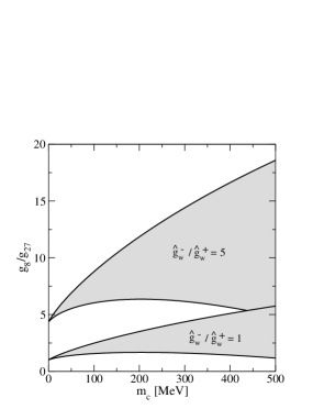
Figure 3: The ratio $g_{8}/g_{27}$ of SU(3) weak couplings in the chiral limit, for two different values of the ratio $\hat{g}_{w}^{-}/\hat{g}_{w}^{+}$ of SU(4) weak couplings in the chiral limit. We have assumed $\Sigma\approx(250\mbox{ MeV})^{3}$, $F\approx 93$ MeV, and varied the scale $\Lambda_{\chi}$, accounting for unknown higher order low-energy couplings, in the range from $\Lambda_{\chi}=1$ GeV (lower edges of the bands) to $\Lambda_{\chi}=4$ GeV (upper edges of the bands).

6 Conclusions

It is generally believed [4, 1, 2] that the charm quark plays an important role in the $\Delta I=1/2$ rule, observed in non-leptonic weak kaon decays, $K\to\pi\pi$. The purpose of this short note has been to investigate one aspect of this role. The philosophy [12] has been to assume that the weak chiral Hamiltonian is known in the unphysical SU(4) limit of a very light charm quark. We then start to increase the charm mass $m_{c}$, taking it eventually to be much larger than $m_{u},m_{d}$ and $m_{s}$, but still small enough such that chiral perturbation theory is applicable. In this limit, the charm quark can be integrated out within an SU(4) chiral effective theory, to obtain an SU(3) chiral effective theory.

We have found that the charm quark does have a distinctive effect on the weak interaction Hamiltonian of this SU(3) theory. The $\Delta I=1/2$ part obtains a logarithmically enhanced contribution, ${\cal O}(m_{c}\ln(1/m_{c}))$, while there are no logarithms in the $\Delta I=3/2$ part, which is at most $\mathcal{O}(m_{c})$ (Eqs. (5.8), (5.9)). Thus, the ratio of $\Delta I=1/2$ and $\Delta I=3/2$ amplitudes departs from the SU(4) limit as $\sim m_{c}\ln(1/m_{c})$. Moreover, the numerical coefficients of the logarithmic contributions are fairly large. The effect comes from penguin-type graphs, the last three in Fig. 2, as suggested by weak coupling considerations a long time ago [4].

The actual values of the 1-loop corrections are, of course, not computable within our framework, because the unknown higher order couplings of the SU(4) chiral Lagrangian enter at the same order. In addition, once the charm quark mass is increased to its physical value, chiral perturbation theory breaks down. Therefore, to really settle from first principles the issue of how important the charm quark is, requires a lattice study [12, 23]. We may note, however, that since Ref. [4] relies on the weak coupling expansion and is thus trustworthy for $m_{c}$ larger than its physical value, while our approach relies on the chiral expansion and is trustworthy for $m_{c}$ smaller than its physical value, the importance of $m_{c}$ is at least confirmed in two complementary limits. Further evidence for its importance comes from the large-$N_{\rm c}$ approach ([13, 14] and references therein), attempting to interpolate between these limits.

To summarise, the results obtained here indicate that together with all the other effects, the dynamics related to the charm quark may play a role in the enhancement observed in $\Delta I=1/2$ decays, providing thus additional motivation for lattice studies.

Appendix Appendix A SU(4) classification

We reiterate in this Appendix some essential aspects of the SU(4) classification of four quark operators. We follow the tensor method discussed, e.g., in Ref. [24]. We also greatly profited from the presentation in Ref. [25].

We start from an operator $O_{rsuv}$, assumed symmetric under $(r\leftrightarrow s,u\leftrightarrow v)$, and transforming under ${\bf 4^{*}}\otimes{\bf 4^{*}}\otimes{\bf 4}\otimes{\bf 4}$ of SU(4). We then define the projected operators

$${O}^{\sigma}_{rsuv} \equiv (P_{1}^{\sigma})_{rsuv;\tilde{r}\tilde{s}\tilde{u}\tilde{v}}\;{O}_{\tilde{r}\tilde{s}\tilde{u}\tilde{v}},$$ (A.1)

$$\hat{O}^{\sigma}_{rsuv} \equiv (P_{2}^{\sigma})_{rsuv;\tilde{r}\tilde{s}\tilde{u}\tilde{v}}\;{O}^{\sigma}_{\tilde{r}\tilde{s}\tilde{u}\tilde{v}},$$ (A.2)

where $\sigma=\pm 1$. Here, with some redundancy in the symmetries of $P_{1}^{\sigma}$,

$$(P_{1}^{\sigma})_{rsuv;\tilde{r}\tilde{s}\tilde{u}\tilde{v}}\equiv{\frac{1}{4}}(\delta_{r\tilde{r}}\delta_{s\tilde{s}}+\sigma\delta_{r\tilde{s}}\delta_{s\tilde{r}})(\delta_{u\tilde{u}}\delta_{v\tilde{v}}+\sigma\delta_{u\tilde{v}}\delta_{v\tilde{u}}),$$ (A.3)

$$(P_{2}^{\sigma})_{rsuv;\tilde{r}\tilde{s}\tilde{u}\tilde{v}}\equiv\delta_{r\tilde{r}}\delta_{s\tilde{s}}\delta_{u\tilde{u}}\delta_{v\tilde{v}}+\frac{1}{(N_{\rm f}+2\sigma)(N_{\rm f}+\sigma)}(\delta_{ru}\delta_{sv}+\sigma\delta_{rv}\delta_{su})\delta_{\tilde{r}\tilde{u}}\delta_{\tilde{s}\tilde{v}}$$

$$~{}~{}~{}~{}~{}~{}~{}~{}-\frac{1}{N_{\rm f}+2\sigma}(\delta_{ru}\delta_{s\tilde{s}}\delta_{v\tilde{v}}\delta_{\tilde{r}\tilde{u}}+\delta_{sv}\delta_{r\tilde{r}}\delta_{u\tilde{u}}\delta_{\tilde{s}\tilde{v}}+\sigma\delta_{rv}\delta_{s\tilde{s}}\delta_{u\tilde{v}}\delta_{\tilde{r}\tilde{u}}+\sigma\delta_{su}\delta_{r\tilde{r}}\delta_{v\tilde{u}}\delta_{\tilde{s}\tilde{v}}),\hskip 28.45274pt$$ (A.4)

where $N_{\rm f}=4$. Let us also denote

$$S^{\sigma} = O^{\sigma}_{klkl},$$ (A.5)

$$R^{\sigma}_{ru} = O^{\sigma}_{rkuk}-\frac{1}{N_{\rm f}}\delta_{ru}S^{\sigma}.$$ (A.6)

Then we can decompose any operator $O_{rsuv}$ into irreducible representations, as

$$O_{rsuv} = \sum_{\sigma=\pm 1}\biggl{[}\hat{O}^{\sigma}_{rsuv}+\frac{1}{N_{\rm f}(N_{\rm f}+\sigma)}(\delta_{ru}\delta_{sv}+\sigma\delta_{rv}\delta_{su})S^{\sigma}$$ (A.7)

$$\hskip 56.9055pt+\frac{1}{N_{\rm f}+2\sigma}(\delta_{ru}R^{\sigma}_{sv}+\delta_{sv}R^{\sigma}_{ru}+\sigma\delta_{rv}R^{\sigma}_{su}+\sigma\delta_{su}R^{\sigma}_{rv})\biggr{]}.$$

Here the representation $\hat{O}^{+}_{rsuv}$ has dimension 84, $\hat{O}^{-}_{rsuv}$ 20, $R^{\pm}_{sv}$’s 15, and $S^{\pm}$ are singlets.

For a sum over irreducible representations with some weights, $c_{rsuv}\hat{O}^{\sigma}_{rsuv}$, we can take advantage of the fact $P_{2}^{\sigma}P_{1}^{\sigma}$ is a projection operator to symmetrise the coefficients:

$$c_{rsuv}\hat{O}^{\sigma}_{rsuv}=\Bigl{[}c_{rsuv}(P_{2}^{\sigma}P_{1}^{\sigma})_{rsuv;\tilde{r}\tilde{s}\tilde{u}\tilde{v}}\Bigr{]}\hat{O}^{\sigma}_{\tilde{r}\tilde{s}\tilde{u}\tilde{v}}\equiv\hat{c}^{\sigma}_{\tilde{r}\tilde{s}\tilde{u}\tilde{v}}\hat{O}^{\sigma}_{\tilde{r}\tilde{s}\tilde{u}\tilde{v}}=\hat{c}^{\sigma}_{\tilde{r}\tilde{s}\tilde{u}\tilde{v}}O_{\tilde{r}\tilde{s}\tilde{u}\tilde{v}}.$$ (A.8)

However, sometimes it may be more convenient not to carry out any symmetrisation.

Finally, we note that in the chiral theory, the matrix $(\partial_{\mu}UU^{\dagger})_{ru}$ is traceless. For the operator ${[{\cal O}_{w}]}_{rsuv}$ in Eq. (2.4), therefore,

$${[{\cal O}_{w}]}_{rkuk}={[{\cal O}_{w}]}_{kskv}=0.$$ (A.9)

Consequently, if we use ${[{\cal O}_{w}]}_{rsuv}$ in the role of $O_{rsuv}$ above,

$${[{\cal O}_{w}]}^{\sigma}_{rkuk}=\frac{\sigma}{2}{[{\cal O}_{w}]}_{rkku},\quad{[{\cal S}_{w}]}^{\sigma}=\frac{\sigma}{2}{[{\cal O}_{w}]}_{lkkl},\quad{[{\cal R}_{w}]}^{+}_{ru}=-{[{\cal R}_{w}]}^{-}_{ru}.$$ (A.10)

Appendix Appendix B SU(3) classification

Let us then consider the SU(3) classification of tensors of the form $\bar{O}_{\bar{r}\bar{s}\bar{u}\bar{v}}$, symmetric under $(\bar{r}\leftrightarrow\bar{s},\bar{u}\leftrightarrow\bar{v})$, and transforming under ${\bf 3^{*}}\otimes{\bf 3^{*}}\otimes{\bf 3}\otimes{\bf 3}$ of SU(3).

The classification of such operators follows almost immediately from Appendix A, by simply replacing $N_{\rm f}\to 3$. There is only one major difference: the antisymmetric tensor $\hat{\!\bar{O}}^{-}_{\bar{r}\bar{s}\bar{u}\bar{v}}$ vanishes identically. The reason is that (as can be understood for instance by contracting with $\epsilon_{\bar{k}\bar{r}\bar{s}}\epsilon_{\bar{l}\bar{u}\bar{v}}$) it corresponds to a representation with dimension 8 just like $\bar{R}^{-}_{\bar{l}\bar{k}}$, but all such representations have already been subtracted by the projection operator in Eq. (A.4).

Consequently, the general reduction now proceeds as

$$\bar{O}_{\bar{r}\bar{s}\bar{u}\bar{v}} = \hat{\!\bar{O}}^{+}_{\bar{r}\bar{s}\bar{u}\bar{v}}+\sum_{\sigma=\pm 1}\biggl{[}\frac{1}{3(3+\sigma)}(\delta_{\bar{r}\bar{u}}\delta_{\bar{s}\bar{v}}+\sigma\delta_{\bar{r}\bar{v}}\delta_{\bar{s}\bar{u}})\bar{S}^{\sigma}$$ (B.1)

$$\hskip 56.9055pt+\frac{1}{3+2\sigma}(\delta_{\bar{r}\bar{u}}\bar{R}^{\sigma}_{\bar{s}\bar{v}}+\delta_{\bar{s}\bar{v}}\bar{R}^{\sigma}_{\bar{r}\bar{u}}+\sigma\delta_{\bar{r}\bar{v}}\bar{R}^{\sigma}_{\bar{s}\bar{u}}+\sigma\delta_{\bar{s}\bar{u}}\bar{R}^{\sigma}_{\bar{r}\bar{v}})\biggr{]},$$

where $\;\hat{\!\bar{O}}^{+}_{\bar{r}\bar{s}\bar{u}\bar{v}}$ transforms under the representation with the dimension 27, and

$$\bar{S}^{\sigma} = \bar{O}^{\sigma}_{\bar{k}\bar{l}\bar{k}\bar{l}},$$ (B.2)

$$\bar{R}^{\sigma}_{\bar{r}\bar{u}} = \bar{O}^{\sigma}_{\bar{r}\bar{k}\bar{u}\bar{k}}-\frac{1}{3}\delta_{\bar{r}\bar{u}}\bar{S}^{\sigma}.$$ (B.3)

Here $\bar{R}^{\pm}_{\bar{r}\bar{u}}$’s have the dimension 8, while $\bar{S}^{\sigma}$ are singlets.

Finally, let us again note that in the chiral theory, i.e. if we replace $\bar{O}_{\bar{r}\bar{s}\bar{u}\bar{v}}\to{[\bar{\cal O}_{w}]}_{\bar{r}\bar{s}\bar{u}\bar{v}}$,

$${[\bar{\cal O}_{w}]}_{\bar{r}\bar{k}\bar{u}\bar{k}}={[\bar{\cal O}_{w}]}_{\bar{k}\bar{s}\bar{k}\bar{v}}=0,$$ (B.4)

so that

$${[\bar{\cal O}_{w}]}^{\sigma}_{\bar{r}\bar{k}\bar{u}\bar{k}}=\frac{\sigma}{2}{[\bar{\cal O}_{w}]}_{\bar{r}\bar{k}\bar{k}\bar{u}},\quad{[\bar{\cal S}_{w}]}^{\sigma}=\frac{\sigma}{2}{[\bar{\cal O}_{w}]}_{\bar{l}\bar{k}\bar{k}\bar{l}},\quad{[\bar{\cal R}_{w}]}^{+}_{\bar{r}\bar{u}}=-{[\bar{\cal R}_{w}]}^{-}_{\bar{r}\bar{u}}.$$ (B.5)

Appendix Appendix C SU(2) classification

We end by considering the SU(2) classification of operators of the type ${Q}_{ijk}$, $i,j,k=1,2$, transforming under ${\bf 2^{*}}\otimes{\bf 2}\otimes{\bf 2}$. We may define ${Q}_{ijk}^{\sigma}=(1/2)({Q}_{ijk}+\sigma{Q}_{ikj})$. Then ${Q}_{ijk}$ can be written as

$${Q}_{ijk}=\hat{Q}_{ijk}^{+}+\sum_{\sigma=\pm 1}\frac{1}{2+\sigma}\Bigl{(}\delta_{ij}{Q}_{llk}^{\sigma}+\sigma\delta_{ik}{Q}_{llj}^{\sigma}\Bigr{)},$$ (C.1)

where $\hat{Q}_{ijk}^{+}$ is traceless, $\hat{Q}_{llk}^{+}=\hat{Q}_{ljl}^{+}=0$. It can be seen to have 4 independent components, and it thus isolates the representation with $I=3/2$.

References

• [1] H. Georgi, Weak Interactions and Modern Particle Theory (Benjamin/Cummings, Menlo Park, California, 1984); J.F. Donoghue, E. Golowich and B.R. Holstein, Dynamics of the Standard Model (Cambridge University Press, Cambridge, 1992).
• [2] A. Pich, Rept. Prog. Phys.  58 (1995) 563 [hep-ph/9502366]; G. Ecker, Prog. Part. Nucl. Phys.  36 (1996) 71 [hep-ph/9511412].
• [3] M.K. Gaillard and B.W. Lee, Phys. Rev. Lett.  33 (1974) 108; G. Altarelli and L. Maiani, Phys. Lett. B 52 (1974) 351; G. Altarelli, G. Curci, G. Martinelli and S. Petrarca, Nucl. Phys. B 187 (1981) 461; A.J. Buras and P.H. Weisz, Nucl. Phys. B 333 (1990) 66.
• [4] M.A. Shifman, A.I. Vainshtein and V.I. Zakharov, Nucl. Phys. B 120 (1977) 316.
• [5] N. Cabibbo, G. Martinelli and R. Petronzio, Nucl. Phys. B 244 (1984) 381; R.C. Brower, G. Maturana, M.B. Gavela and R. Gupta, Phys. Rev. Lett.  53 (1984) 1318.
• [6] A. Pich, B. Guberina and E. de Rafael, Nucl. Phys. B 277 (1986) 197; A. Pich and E. de Rafael, Nucl. Phys. B 358 (1991) 311.
• [7] T.N. Truong, Phys. Lett. B 207 (1988) 495.
• [8] J. Kambor, J. Missimer and D. Wyler, Nucl. Phys. B 346 (1990) 17; G. Ecker, J. Kambor and D. Wyler, Nucl. Phys. B 394 (1993) 101.
• [9] J. Gasser and U.G. Meissner, Phys. Lett. B 258 (1991) 219.
• [10] J. Kambor, J. Missimer and D. Wyler, Phys. Lett. B 261 (1991) 496; J. Kambor, J.F. Donoghue, B.R. Holstein, J. Missimer and D. Wyler, Phys. Rev. Lett.  68 (1992) 1818; J. Bijnens, E. Pallante and J. Prades, Nucl. Phys. B 521 (1998) 305 [hep-ph/9801326]; E. Pallante, JHEP 01 (1999) 012 [hep-lat/9808018].
• [11] E. Pallante and A. Pich, Phys. Rev. Lett.  84 (2000) 2568 [hep-ph/9911233]; Nucl. Phys. B 592 (2001) 294 [hep-ph/0007208]; V. Cirigliano, G. Ecker, H. Neufeld and A. Pich, Eur. Phys. J. C 33 (2004) 369 [hep-ph/0310351].
• [12] L. Giusti, P. Hernández, M. Laine, P. Weisz and H. Wittig, hep-lat/0407007.
• [13] W.A. Bardeen, A.J. Buras and J.-M. Gérard, Phys. Lett. B 180 (1986) 133; Nucl. Phys. B 293 (1987) 787; Phys. Lett. B 192 (1987) 138.
• [14] T. Hambye, S. Peris and E. de Rafael, JHEP 05 (2003) 027 [hep-ph/0305104].
• [15] C.W. Bernard, T. Draper, A. Soni, H.D. Politzer and M.B. Wise, Phys. Rev. D 32 (1985) 2343.
• [16] J. Gasser and H. Leutwyler, Annals Phys.  158 (1984) 142; Nucl. Phys. B 250 (1985) 465.
• [17] J. Bijnens, G. Ecker and J. Gasser, hep-ph/9411232.
• [18] S. Descotes-Genon, N.H. Fuchs, L. Girlanda and J. Stern, Eur. Phys. J. C 34 (2004) 201 [hep-ph/0311120].
• [19] L. Giusti, C. Hoelbling, M. Lüscher and H. Wittig, Comput. Phys. Commun.  153 (2003) 31 [hep-lat/0212012].
• [20] P. Hernández and M. Laine, JHEP 01 (2003) 063 [hep-lat/0212014].
• [21] G. Colangelo and E. Pallante, Nucl. Phys. B 520 (1998) 433 [hep-lat/9708005].
• [22] R.J. Crewther, Nucl. Phys. B 264 (1986) 277.
• [23] For a review of the current status of lattice studies see, e.g., A. Soni, Pramana 62 (2004) 415 [hep-ph/0307107].
• [24] H. Georgi, Lie Algebras in Particle Physics (Benjamin/Cummings, Reading, Massachusetts, 1982).
• [25] M. Lüscher, Irreducible representations of SU(4), private notes, 2002 (unpublished).