Holes in the ghost condensate

Abstract

In a recently proposed model of “ghost condensation”, spatially homogeneous states may mix, via tunneling, with inhomogeneous states which are somewhat similar to bubbles in the theory of false vacuum decay, the corresponding bubble nucleation rate being exponentially sensitive to the ultraviolet completion of the model. The conservation of energy and charge requires that the energy density is negative and the field is strongly unstable in a part of the nucleated bubble. Unlike in the theory of false vacuum decay, this region does not expand during subsequent real-time evolution. In the outer part, positive energy outgoing waves develop, which eventually form shocks. Behind the outgoing waves and away from the bubble center, the background settles down to its original value. The outcome of the entire process is thus a microscopic region of negative energy and strong field — “hole in the ghost condensate” — plus a collection of outgoing waves (particles of the ghost condensate field) carrying away finite energy.

I Introduction and summary

In view of the evidence for the accelerated expansion of the Universe, several attempts have been made recently to construct models in which gravity is modified at large distances Charmousis:1999rg ; Kogan:1999wc ; DGP ; Jacobson:2001yj ; Freese:2002sq ; Carroll:2003wy ; AH ; Holdom:2004yx . One approach, dubbed ghost condensation AH , invokes a scalar field with unconventional kinetic term, like in models of k-essence Armendariz-Picon:2000dh but with the action depending on the derivatives only,

$$S=M^{4}\int~{}d^{4}x~{}P(X)$$ (1)

where

$$X=\partial^{\mu}\phi\partial_{\mu}\phi$$

(space-time signature $(+,-,-,-)$). One views this model as an effective theory valid at energies below some cutoff. Assuming that $P^{\prime}(0)<0$, excitations about a state $\phi=0$ are ghosts, hence the name of the model. A proptotype example of the “potential” having this property is

$$P(X)=\frac{1}{2}(X-1)^{2}$$ (2)

When gravity is switched off, the scalar theory is perturbatively stable provided that the background has the Lorentz-violating form,

$$\phi=ct$$ (3)

where the constant $c$ is such that

$$P^{\prime}(c^{2}) \geq 0$$ (4)

$$2P^{\prime\prime}(c^{2})c^{2}+P^{\prime}(c^{2}) \geq 0$$ (5)

(for the potential (2) these inequalities imply $c\geq 1$). Cosmological evolution drives the field to a special point

$$c=c_{*}$$ (6)

where

$$P^{\prime}(c_{*}^{2})=0$$

($c_{*}=1$ for the potential (2)). At the level of small perturbations about this background, the model has interesting phenomenology, as discussed in Refs. AH ; Dubovsky:2004qe ; Peloso:2004ut .

There are several points to discuss beyond the perturbation theory. One is the behavior of the ghost condensate near sources of strong gravitational field, e.g., near black holes Frolov:2004vm . In this paper we address another issue, namely, quantum stability of the ghost condensate. As we discuss in Section 2, even in the absence of gravitational interactions, there exist inhomogeneous configurations of the scalar field, bubbles, with which the state (3) can mix via tunneling. We will see that the tunneling exponent is dominated by the ultraviolet (UV) properties of the theory, so the decay rate is exponentially sensitive to the UV completion of the model, in accord with Ref. AH . If the UV cutoff is well below the scale $M$, the bubble nucleation rate is small.

Still, it is of interest to understand the further evolution of the bubbles which can nucleate via tunneling. In conventional scalar theories with false vacua (local minima of the scalar potential), a bubble of the true vacuum, once created, expands practically with the speed of light Kobzarev:1974cp ; Coleman:1977py , and the true vacuum eventually occupies the entire space. The difference between the energies of the false and true vacua is released into the bubble wall, whose energy thus tends to infinity at asymptotically large time. We will see in Section 3 that in the ghost condensation model the situation is quite different. In the central part of a bubble, the energy density is negative and, furthermore, the condition (4) (and also (5)) is violated. The system is unstable there, so the ultimate fate of the field in this region cannot be understood in the UV-incomplete theory. The point, however, is that this part does not expand and remains of microscopic size at all times; this is a “hole in the ghost condensate”. Moreover, there is no energy flow through the boundary of this hole, so the hole has little, if any, effect on the outer part of the bubble.

In the outer part, a shock wave (or series of shock waves) is formed which propagates outwards. At the level of classical field theory with the action (1), the formation of a shock wave means a singularity after which the solution ceases to exist. Resolving this singularity would be possible in UV complete theory only. Assuming that the singularity is smoothened out by the UV effects, we study the entire evolution of the bubble. We find that the ghost condensate behind the shock wave settles down to its original value, $\dot{\phi}=c$, $\vec{\nabla}\phi=0$, so the energy of the shock wave does not increase in time. Therefore, the amplitude of the shock wave decreases in time; in the quantum theory the wave ultimately decays into quanta of the “ghost field” $\phi$. In the case of the special background (6) all these properties follow from the energy conservation, while for the general initial background $\dot{\phi}=c>c_{*}$ we have found them by numerical simulations.

The outcome of the entire process is thus the hole in the ghost condensate, a microscopic region (of the size set by the length scale $M^{-1}$ and/or the UV cutoff) where the energy density is negative, and the field strongly deviates from its background value. These holes in the ghost condensate are likely to antigravitate.

II Nucleated bubbles

The energy functional of the model is

$$E=\int~{}d^{3}x~{}[2P^{\prime}(X)\dot{\phi}^{2}-P(X)]$$ (7)

Besides the energy, there is another conserved quantity, the charge. Indeed, the field equation has the form of current conservation,

$$\partial_{\mu}[P^{\prime}(X)\partial^{\mu}\phi]=0$$ (8)

which implies the conservation of the charge

$$Q=\int~{}d^{3}x~{}P^{\prime}(X)\dot{\phi}$$ (9)

It is precisely charge conservation that renders the background (3) stable against small perturbations: even though for arbitrary perturbation the energy can decrease, small perturbations in the same charge sector have larger energy than the background itself.

Figure 1: An example of a configuration with vanishing energy and charge.

Figure 2: A bubble at the moment of nucleation.

The latter property does not hold for large perturbations, so the state (3) may tunnel into other configurations which have the same energy and charge. To be specific, let us consider the background

$$c=c_{*}$$ (10)

(the generalization to $c>c_{*}$ is straightforward provided that $c$ is not very large, otherwise one should consider trial configurations with non-zero spatial gradient). This configuration has

$$Q=0\;,\;\;\;E=0$$

so final states the system can tunnel into have zero energy and charge. An example of such a state is a spherically symmetric configuration with zero spatial gradient, $\vec{\nabla}\phi=0$, while the time derivative is a combination of step functions (see fig. 1)

$$\dot{\phi} = c_{1}\;\;\mbox{at}\;0<r<a$$

$$\dot{\phi} = c_{2}\;\;\mbox{at}\;a<r<b$$

$$\dot{\phi} = c_{*}\;\;\mbox{at}\;r>b$$ (11)

with $0<c_{1}<c_{*}$, $c_{2}>c_{*}$. The charge and energy of this configuration are

$$\frac{3}{4\pi}Q = a^{3}P^{\prime}(c_{1}^{2})\cdot c_{1}+(b^{3}-a^{3})P^{\prime}(c_{2}^{2})\cdot c_{2}$$

$$\frac{3}{4\pi}E = a^{3}[2P^{\prime}(c_{1}^{2})\cdot c_{1}^{2}-P(c_{1}^{2})]$$

$$+(b^{3}-a^{3})[2P^{\prime}(c_{2}^{2})\cdot c_{2}^{2}-P(c_{2}^{2})]$$

The first term in $Q$ is negative, while the second is positive (this is why the region with $c_{2}>c_{*}$ is needed). Requiring that $Q=0$ one finds

$$b^{3}-a^{3}=-a^{3}\cdot\frac{P^{\prime}(c_{1}^{2})\cdot c_{1}}{P^{\prime}(c_{2}^{2})\cdot c_{2}}$$

so one obtains for the energy

$$E=-a^{3}\cdot P^{\prime}(c_{1}^{2})\cdot c_{1}\cdot[F(c_{2})-F(c_{1})]$$

where

$$F(c)=\frac{2P^{\prime}(c^{2})\cdot c^{2}-P(c^{2})}{P^{\prime}(c^{2})\cdot c}$$

For wide class of potentials, including (2), the function $F$ is positive at all $c$, has a minimum at some point $c_{**}$ on the left of the minimum of $P$, i.e., $0<c_{**}<c_{*}$, and diverges as $c\to+0$ or $c\to+\infty$.

As a side remark, the minimum of $F$ occurs at the point where

$$2P^{\prime\prime}(c_{**}^{2})c_{**}^{2}+P^{\prime}(c_{**}^{2})=0$$

It is straightforward to see that in the absence of gravity, small perturbations about the homogeneous background (3) grow exponentially for $c_{**}<c<c_{*}$ (tachyonic region) and oscillate for $c<c_{**}$ and $c>c_{*}$ (in the former region they have negative energy).

For $c_{1}<c_{**}$ (that is, necessarily left of the tachyonic region) and sufficiently close to $+0$, there exists a point $c_{2}>c_{*}$ such that

$$F(c_{2})=F(c_{1})$$

With this choice of $c_{1}$ and $c_{2}$, both energy and charge are indeed equal to zero. The system can tunnel into such a configuration. Further evolution will lead to non-zero spatial gradient of $\phi$, because $\dot{\phi}$ is inhomogeneous in space for the trial configuration just constructed. Note that only the ratio $a/b$ is determined by the energy and charge, while the overall spatial scale remains a free parameter; this means that the conservation of energy and charge allow for creation of bubbles of arbitrary size.

It is worth noting that the step-function configuration of fig. 1 has been chosen for illustration purposes only. The nucleated bubbles need not have steep walls. In what follows we have in mind smooth bubble profile at the moment of nucleation, as shown in fig. 2.

The initial and final states of tunneling are somewhat unconventional here, since the field configurations are time-dependent. Also, when describing tunneling, one has to impose a constraint of charge conservation. The semiclassical formalism relevant in this situation was in fact developed some time ago Lee:1988ge ; Coleman:1989zu . The bottom line is that one perfoms the Wick rotation to the Euclidean space-time, and considers pure imaginary fields there,

$$\phi=-i\theta$$ (12)

where $\theta$ is real. The boundary conditions at initial and final Euclidean time, $\tau_{i}=-\infty$ and $\tau_{f}=0$, respectively, require that the field be homogeneous in space,

$$\vec{\nabla}\theta(\tau_{i,f})=0$$ (13)

the latter condition being trivially satisfied for the initial state (3), since at large negative times $\theta(\vec{x},\tau)=i\phi(\vec{x},t=-i\tau)=c\tau$. Generally speaking, the semiclassical tunneling exponent equals the Euclidean action evaluated on a solution to the Euclidean field equations obeying the relations (12) and (13). In the model at hand, the Euclidean action is still given by eq. (1), where now

$$X=(\partial_{\mu}\theta)^{2}$$

and metric is Euclidean.

It is straightforward to see, however, that the model (1) as it stands does not have relevant Euclidean solutions. Indeed, under rescaling

$$\theta(x^{\mu})\to\lambda\theta(\lambda^{-1}x^{\mu})$$

the boundary conditions (13) and the initial configuration $\theta=c\tau$ do not change, while the action scales as

$$S\to\lambda^{4}S$$

Thus, there are no relevant saddle points; configurations of small size have small Euclidean action.

The scaling argument tells that the bubble nucleation rate is UV dominated. If the UV cutoff $\Lambda$ is smaller than $M$, the decay exponent is large,

$$S\sim\left(\frac{M}{\Lambda}\right)^{4}$$ (14)

so the decay rate is small, in accord with the analysis in Ref. AH .

III Real time evolution

III.1 Classical evolution in (1+1)-dimensions

III.1.1 Legendre transformation

To understand how configurations of the type shown in fig. 2 evolve in Minkowski space-time, let us first neglect the spatial curvature of the bubble walls, and thus consider the system with the action (1) in $(1+1)$ dimensions. The explicit form of the field equation (8) in $(1+1)$ dimensions is

$$(P^{\prime}+2P^{\prime\prime}\phi_{,t}^{2})\phi_{,tt}-4P^{\prime\prime}\phi_{,x}\phi_{,t}\phi_{,xt}-(P^{\prime}-2P^{\prime\prime}\phi_{,x}^{2})\phi_{,xx}=0$$ (15)

Here and in the following comma denotes differentiation. This non-linear equation is simplified by the Legendre transformation. Instead of $x$, $t$, one chooses new independent variables

$$\xi = \phi_{,t}$$

$$\eta = \phi_{,x}$$ (16)

and, instead of $\phi$, one considers an unknown function

$$u(\xi,\eta)=-\phi+t\xi+x\eta$$

This change of variables is legitimate in any region where the pairs of coordinates $(\xi,\eta)$ and $(x,t)$ are in one-to-one correspondence. Equivalently, in such a region the Jacobian of the coordinate transformation,

$$J=u_{,\xi\xi}u_{,\eta\eta}-(u_{,\xi\eta})^{2}$$ (17)

is nowhere zero or infinite. The second derivatives are

$$\phi_{,tt} = J^{-1}\cdot u_{,\eta\eta}$$

$$\phi_{,xt} = -J^{-1}\cdot u_{,\xi\eta}$$

$$\phi_{,xx} = J^{-1}\cdot u_{,\xi\xi}$$ (18)

while the original coordinates are related to $\xi$ and $\eta$ as follows,

$$t = u_{,\xi}$$ (19)

$$x = u_{,\eta}$$ (20)

The original equation (15) in terms of new variables takes the form

$$(P^{\prime}+2P^{\prime\prime}\xi^{2})u_{,\eta\eta}+4P^{\prime\prime}\xi\eta u_{,\xi\eta}-(P^{\prime}-2P^{\prime\prime}\eta^{2})u_{,\xi\xi}=0$$ (21)

where $P$ is a function of the combination $(\xi^{2}-\eta^{2})$. This is now a linear equation with coefficients that depend on the coordinates $\xi$, $\eta$. Once a solution $u(\xi,\eta)$ is found, the quantities of interest $\phi_{,t}\equiv\xi(x,t)$ and $\phi_{,x}\equiv\eta(x,t)$ are obtained, at least in principle, by inverting eqs. (19), (20).

To simplify eq. (21), let us take advantage of its Lorentz invariance and introduce new variables $\rho$ and $\theta$ related to $\xi$ and $\eta$ as follows,

$$\xi\equiv\phi_{,t} = \rho\cosh\theta$$ (22)

$$\eta\equiv\phi_{,x} = \rho\sinh\theta$$ (23)

(of course, we made an assumption here that $|\phi_{,t}|>|\phi_{,x}|$; it is valid in all cases we consider). Clearly, the meaning of $\rho$ is that it is a scalar

$$\rho=\sqrt{(\partial_{\mu}\phi)^{2}}\equiv\sqrt{X}$$

In terms of the variables $\rho$ and $\theta$, the original coordinates are

$$t = u_{,\rho}\cosh\theta-\frac{1}{\rho}u_{,\theta}\sinh\theta$$ (24)

$$x = -u_{,\rho}\sinh\theta+\frac{1}{\rho}u_{,\theta}\cosh\theta$$ (25)

Now eq. (21) reads

$$\frac{P^{\prime}+2P^{\prime\prime}\rho^{2}}{\rho^{2}}u_{,\theta\theta}-P^{\prime}u_{,\rho\rho}-\frac{P^{\prime}+2P^{\prime\prime}\rho^{2}}{\rho}u_{,\rho}=0$$ (26)

where $P=P(\rho^{2})$, and prime still denotes the derivative with respect to its argument $\rho^{2}$.

This equation is hyperbolic when $P^{\prime}$ and $(P^{\prime}+2P^{\prime\prime}\rho^{2})$ have the same sign, i.e., when the small perturbations of the field $\phi$ do not grow (no tachyons). This equation is elliptic in the tachyonic region, and has singularities (zeroes in front of one of the second derivative terms) on the boundary of that region, i.e., at $P^{\prime}=0$ and at $P^{\prime}+2P^{\prime\prime}\rho^{2}=0$. The second boundary point is not of interest for our purposes; about the first boundary point we will have to say more later.

Let us consider the region on the right of the minimum of $P$, where both $P^{\prime}$ and $P^{\prime\prime}$ are positive. The final simplification of eq. (26) is made by introducing a new variable $\tau$ instead of $\rho$,

$$\tau=\int_{c_{*}}^{\rho}~{}d\rho~{}\sqrt{\frac{P^{\prime}+2P^{\prime\prime}\rho^{2}}{P^{\prime}\rho^{2}}}$$ (27)

where for future convenience the constant of integration is chosen in such a way that

$$\tau(\rho=c_{*})=0$$

Then instead of eq. (26) one obtains

$$u_{,\theta\theta}-u_{,\tau\tau}-F(\tau)u_{,\tau}=0$$ (28)

where

$$F(\tau)=\frac{\tau_{,\rho\rho}}{\tau_{,\rho}^{2}}+\rho\tau_{,\rho}$$

It is instructive to point out that near the point $c_{*}$ one has

$$P^{\prime}=\mbox{const}\cdot(\rho^{2}-c_{*}^{2})$$

Then the above expressions have simple form. In particular,

$$\tau=2\sqrt{\frac{\rho-c_{*}}{c_{*}}}$$ (29)

and eq. (28) reads

$$u_{,\theta\theta}-u_{,\tau\tau}-\frac{1}{\tau}u_{,\tau}=0$$ (30)

The latter equation has the form of the wave equation in $(2+1)$ dimensions for $O(2)$-symmetric functions.

III.1.2 Shock waves

Let us consider initial data such that $\phi_{,x}=0$ everywhere (cf. eq. (13)) and $\phi_{,t}>c_{*}$, i.e., $P^{\prime}$ and $P^{\prime\prime}$ are positive on an entire line $-\infty<x<+\infty$. Let us further assume that $\phi_{,t}$ at $t=0$ is a monotonically increasing function of $x$, which tends to certain finite values as $x\to\pm\infty$,

$$\phi_{,t}(t=0,x\to-\infty) \to \rho_{-}$$ (31)

$$\phi_{,t}(t=0,x\to+\infty) \to \rho_{+}$$ (32)

with

$$\rho_{+}>\rho_{-}\geq c_{*}$$

This initial configuration is shown in fig. 3, and it corrsponds to the outer part of the bubble, namely, the region $r\gtrsim b$ for the configuration of fig. 2. To this end, $x$ is to be identified with $-r$ (thus, the bubble is meant to be on the right in fig. 3; this somewhat bizarre convention simplfies the further discussion).

Figure 3: Initial data in the outer region of a bubble.

These initial data are translated into the Legendre variables as follows. According to eqs. (23), (24) and (25), the initial condition $\phi_{,x}=0$ is satisfied when the line $t=0$ coincides with the line $\theta=0$, and $u=\mbox{const}$ on that line. Thus, the initial data are

$$u_{,\theta} \neq 0\;,\;\;\;\;\theta=0$$ (33)

$$u_{,\rho} = 0\;,\;\;\;\;\theta=0$$ (34)

Once the initial data $\phi_{,t}(t=0,x)$ is specified, the initial data for the Legendre variables is obtained by inverting the relations

$$\rho = \phi_{,t}(t=0,x)$$

$$x = \frac{1}{\rho}u_{,\theta}(\theta=0,\rho)$$ (35)

According to eqs. (22) and (31), (32), the initial data for $u_{,\theta}$ are specified on a finite interval

$$\rho_{-}<\rho<\rho_{+}$$ (36)

Since $\phi_{,t}$ at $t=0$ is an increasing function of $x$, eq. (35) means that $u_{,\theta}$ at $\theta=0$ is an increasing function of $\rho$. Since $x$ runs from $-\infty$ to $+\infty$, eq. (35) implies that $u_{,\theta}$ is singular at the ends of the interval (36),

$$u_{,\theta}(\theta=0,\rho\to\rho_{-}) \to -\infty$$ (37)

$$u_{,\theta}(\theta=0,\rho\to\rho_{+}) \to +\infty$$ (38)

Instead of $\rho$, one can of course use the coordinate $\tau$ in the above expressions.

Figure 4: Singularity lines in $(\tau,\theta)$-plane.

Let us now discuss the behavior of the solution $u(\tau,\theta)$ to eq. (28), in the $(\tau,\theta)$ plane. The singularities (37) and (38) that start at $\tau_{-}$ and $\tau_{+}$, respectively, move along the light-like lines on this plane. The relevant light-like lines are the lines L and R in fig. 4 (the other two lines are screened by the lines L and R).

The right singularity, labeled R in fig. 4, occurs at

$$\theta=\tau_{+}-\tau$$ (39)

Near the right singularity the function $u$ has the form

$$u=A(\tau)C_{+}(\theta+\tau)$$ (40)

where $A(\tau)$ is a slowly varying function, while $C_{+}(\bar{z}\equiv(\theta+\tau))$ varies rapidly and has the property

$$C_{+}(\bar{z})\to+\infty\;,\;\;\;\bar{z}\to\tau_{+}-0$$

The form of $C_{+}$ is determined by the singular part of the initial configuration $u_{,\theta}(\theta=0,\rho)$ as $\rho\to\rho_{+}$, i.e., by the behavior of $\phi_{,t}(t=0,x)$ as $x\to+\infty$.

¿From eqs. (24) and (25) one finds that near the right singularity

$$t = \frac{A(\tau)}{\rho(\tau)}C_{+}^{\prime}(\theta+\tau)(\rho\,\tau_{,\rho}\cosh\theta-\sinh\theta)$$ (41)

$$x = \frac{A(\tau)}{\rho(\tau)}C_{+}^{\prime}(\theta+\tau)(-\rho\,\tau_{,\rho}\sinh\theta+\cosh\theta)$$ (42)

Note that from eq. (27) it follows that $\rho\,\tau_{,\rho}>1$, so time $t$ is positive near the right singularity. The coordinate $x$ is also positive near the right singularity, at least in the lower right corner of fig. 4, where $\theta$ is small. Thus, the lower right part of the line R corresponds to the asymptotics $t\to\infty$, $x\to+\infty$.

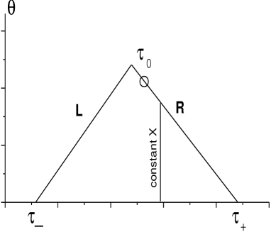
Figure 5: Line of constant $(\partial_{\mu}\phi)^{2}$ in $(\tau,\theta)$-plane.

A line of constant $\tau$, i.e., a line of constant $X\equiv(\partial_{\mu}\phi)^{2}$, shown in fig. 5, hits the singularity. According to eqs. (41) and (42), at large $t$ and $x$ this line becomes a straight line in $(x,t)$-plane, with the slope

$$\frac{x}{t}=\frac{\cosh(\tau_{+}-\tau)-\rho\,\tau_{,\rho}\sinh(\tau_{+}-\tau)}{\rho\,\tau_{,\rho}\cosh(\tau_{+}-\tau)-\sinh(\tau_{+}-\tau)}$$ (43)

where we made use of the relation (39) to express $\theta$ through $\tau$. For $\tau$ sufficiently close to $\tau_{+}$, the lines of constant $X$ move towards positive $x$, so there is a wave moving right. In the case of the bubble of fig. 2 this wave moves inwards the bubble.

For generic initial data there is a point on the right singularity line R where the two terms in the numerator in eq. (43) cancel each other (shown by a circle in fig. 5). Then left of this point (i.e., at $\tau<\tau_{0}$) the coordinate $x$ is negative (and tends to $-\infty$ as the line of constant $\tau$ approaches the singularity line). In this region, the lines of constant $(\partial_{\mu}\phi)^{2}$ move left, so there is a left-moving wave. In between the left-moving and right-moving waves, the space is gradually occupied by “constant” ghost condensate

$$\phi_{,t} = \rho(\tau_{0})\cosh(\tau_{+}-\tau_{0})$$

$$\phi_{,x} = \rho(\tau_{0})\sinh(\tau_{+}-\tau_{0})$$ (44)

The final point to mention about the right singularity line is that the slope (43) increases as $\rho$ increases, so the lines of constant $X$ do not intersect on $(x,t)$-plane, see fig. 6. Indeed, one finds

$$\left(\frac{x}{t}\right)_{,\rho} = \frac{2\rho^{3}}{\sqrt{1+2P^{\prime\prime}\rho^{2}/P^{\prime}}}$$ (45)

$$\times\frac{1}{[\rho\,\tau_{,\rho}\cosh(\tau_{+}-\tau)-\sinh(\tau_{+}-\tau)]^{2}}$$

$$\times\left(3\frac{P^{\prime\prime 2}}{P^{\prime 2}}-\frac{P^{\prime\prime\prime}}{P^{\prime}}\right)$$

which is positive for large class of the potentials $P$. As it evolves, the wave gets spread over larger interval of $x$. The asymptotic velocity of the wave is always smaller than the speed of light: the maximum slope (43) is attained in the lower right corner where $\tau\approx\tau_{+}$ and $\theta\approx 0$, and there

$$\frac{x}{t}=\frac{1}{(\rho\,\tau_{,\rho})(\tau_{+})}<1$$

For initial data close to the minimum of $P$, the maximum slope, and hence the velocity of the wave are small, since $\rho\,\tau_{,\rho}$ is large, see eq. (29).

Figure 6: Lines of constant $X\equiv(\partial_{\mu}\phi)^{2}$ in $(x,t)$-plane. Regions R and L correspond at large $t$ to regions near the lines R and L in fig. 4.

Let us turn to the left singularity line L. This line corresponds to

$$\theta=\tau-\tau_{-}$$

and the solution near the singularity line has the form, cf. eq. (40),

$$u=A(\tau)C_{-}(\tau-\theta)$$ (46)

The function $C_{-}$ is rapidly varying; it is an increasing function of its argument with the property

$$C_{-}(z)\to-\infty\;,\;\;\;\;z\equiv(\tau-\theta)\to\tau_{-}+0$$

At the very first sight the situation here is similar to that near the line R. This is not quite true, however. The expressions for $t$ and $x$ near the line L (analogs of eqs. (41) and (42)) are

$$t = \frac{A(\tau)}{\rho(\tau)}C_{-}^{\prime}(\tau-\theta)(\rho\,\tau_{,\rho}\cosh\theta+\sinh\theta)$$ (47)

$$x = -\frac{A(\tau)}{\rho(\tau)}C_{-}^{\prime}(\tau-\theta)(\rho\,\tau_{,\rho}\sinh\theta+\cosh\theta)$$ (48)

Time $t$ is again positive while $x$ is now negative. Thus the left part of fig. 4 describes a wave moving left. In the context of a bubble of fig. 2 this wave moves outwards.

The point, however, is that the absolute values of the slopes of lines of constant $\tau$ (i.e., constant $X$) on the $(x,t)$-plane increase as $\rho$ increases: the relevant formula is again given by eq. (45), but with the opposite overall sign (the wave moves left) and with $(\tau-\tau_{-})$ substituted for $(\tau_{+}-\tau)$. Thus, at given large $t$, points (in $x$-space) with larger $\rho$ are to the left of points with smaller $\rho$. On the other hand, at $t=0$ the situation is opposite, since the initial data are such that $\phi_{,t}=\rho$ increases with $x$ as shown in fig. 3. This means that lines of constant $X$ intersect on $(x,t)$-plane, see fig. 6. Of course, the whole treatment breaks down when these lines intersect, as there emerges a singularity on $(x,t)$-plane. This singularity is of the type of shock wave, or kink, at which the first derivatives $\phi_{,t}$ and $\phi_{,x}$ are step functions: just before the lines of constant $X$ intersect, the values of $X(x)$, and hence $\phi_{,t}$ and $\phi_{,x}$ are substantially different at neighboring points of space. From the above analysis it follows that this shock wave moves left in fig. 3, at least at the moment when it gets formed — in the context of a bubble this is the motion outwards.

III.1.3 Numerical analysis

Equation (15) for the evolution of the ghost field can be studied numerically. For the purpose, we found it convenient to take $\xi=\phi_{,t}$ and $\eta=\phi_{,x}$ as new dependent field variables. In terms of these, the equation of motion can be recast into the form

$$(P^{\prime}+2P^{\prime\prime}\xi^{2})\xi_{,t}-4P^{\prime\prime}\eta\xi\xi_{,x}-(P^{\prime}-2P^{\prime\prime}\eta^{2})\eta_{,x}=0$$ (49)

where $P=P(\xi^{2}-\eta^{2})$, with the additional constraint

$$\eta_{,t}=\xi_{,x}$$ (50)

We discretize now the space dependence of the variables $\xi,\eta$ by introducing a lattice with uniform lattice spacing $a$ and defining

$$\xi_{n} = \xi(na)$$

$$\eta_{n} = \eta(na)$$ (51)

We also make the overall lattice finite imposing $-N\leq n\leq N$, introduce Neumann boundary conditions on $\phi$, and replace the derivatives $\xi_{,x},\eta_{,x}$ with their central difference approximations $(\nabla\xi)_{n}=(\xi_{n+1}-\xi_{n-1})/(2a),(\nabla\eta)_{n}=(\eta_{n+1}-\eta_{n-1})/(2a)$. After these steps eqs. (49), (50) take the form of a set of coupled ordinary differential equations of the first order for the time dependence of the variables $\xi_{n},\eta_{n}$:

$$\frac{d\xi}{dt} = \frac{4P^{\prime\prime}\eta\xi\nabla\xi+(P^{\prime}-2P^{\prime\prime}\eta^{2})\nabla\eta}{(P^{\prime}+2P^{\prime\prime}\xi^{2})}$$ (52)

$$\frac{d\eta}{dt} = \nabla\xi$$ (53)

We integrated these equations in time by using the second order Runge-Kutta formula.

We would like to make a few observations about our numerical procedure. The main concern in integrating evolution equations such as the ones at hand is the possible onset of numerical instabilities. The avoidance of such instabilities limits the maximum time step to values that are generally small enough to render the use of higher order integration formulae unwarranted. This is why we used the second order Runge-Kutta algorithm. The adequacy of this algorithm was confirmed by the conservation of energy, which, in the stability region, was accurate to better that one part per million. However, the time integration can become unstable. This happens a) when the formation of a shock wave generates a wave-front spanning only a few lattice spacings and b) when the signature of the equation is elliptic over some domain of values of $x$. In the case (a) the approximation to the space derivative obviously fails, and this leads to instabilities in the time integration. We have noticed, incidentally, that the onset of such instabilities is more serious if one uses $\phi$ itself, rather than $\eta=\phi_{,x}$, as one of the independent variables. The use of $\eta$ avoids the need of discretizing second derivatives with respect to $x$ and leads to a better behaved integration algorithm. From the physical point of view, one can also argue that $\phi_{,x}$ plays a more fundamental role than $\phi$ in the system under consideration.

The instabilities that occur in the case (b), namely in the domains where the equation is elliptic, are of physical nature, and not caused by shortcomings of the integration procedure. Indeed, with an elliptic equation, perturbations grow exponentially when one integrates the equation forward in time. The damping of such instabilities would be left to the UV completion of the theory.

Whether due to a shock wave or to a domain of elliptic signature, numerical instabilities are characterized by an exponential growth of the short range fluctuations. In order to tame such instabilities we supplemented our evolution algorithm with an additional step, which serves to dampen the growth of those fluctuations. Namely, after the standard Runge-Kutta integration step, we use a fast Fourier transform (FFT) to calculate

$$\tilde{\xi}_{k} = \sum_{n}e^{2\pi\imath kn/N}\,\xi_{n}$$

$$\tilde{\eta}_{k} = \sum_{n}e^{2\pi\imath kn/N}\,\eta_{n}$$ (54)

and dampen $\tilde{\xi},\tilde{\eta}$ by replacing

$$\tilde{\xi}_{k} \to \tilde{\xi}_{k}^{\prime}=e^{-\alpha[1-\cos(2\pi k/N)]\,dt/a^{2}}\,\tilde{\xi}_{k}$$

$$\tilde{\eta}_{k} \to \tilde{\eta}_{k}^{\prime}=e^{-\alpha[1-\cos(2\pi k/N)]\,dt/a^{2}}\,\tilde{\eta}_{k}$$ (55)

$dt$ being the integration time step and $\alpha$ suitable parameter. After this step, we go back to the original variables by the inverse FFT.

We have found that, with a judicious choice of the damping factor $\alpha$, we were able to evolve the equations well past the formation of the shock wave and also for some time in the presence of an elliptic domain, while preserving the conservation of energy to a few per cent, or better. Of course, the front of the shock gets slightly smoothed out and, in the elliptic domain, the short range fluctuations, after some initial wild growth, get gradually damped down and become intolerable only at relatively late times. It is interesting to observe that our procedure, while mainly motivated by the desire to keep the numerical integration under control, could also be thought of as a way to mimic the effects of the UV completion.

Finally, the discretization of the equations for the three-dimensional evolution with spherical symmetry proceeds along the same lines, after having inserted the appropriate metric factors (powers of $r$).

In fig. 7 we show the profile of the field configuration obtained by solving eq. (15) numerically, with the potential $P$ given by eq. (2) and initial data similar to those shown in fig. 3. This solution clearly demonstrates the formation of the shock wave and its motion to the left. There is also a soft wave slowly propagating to the right. In our numerical simulations we always observed this behavior of solutions for initial data of the type shown in fig. 3.

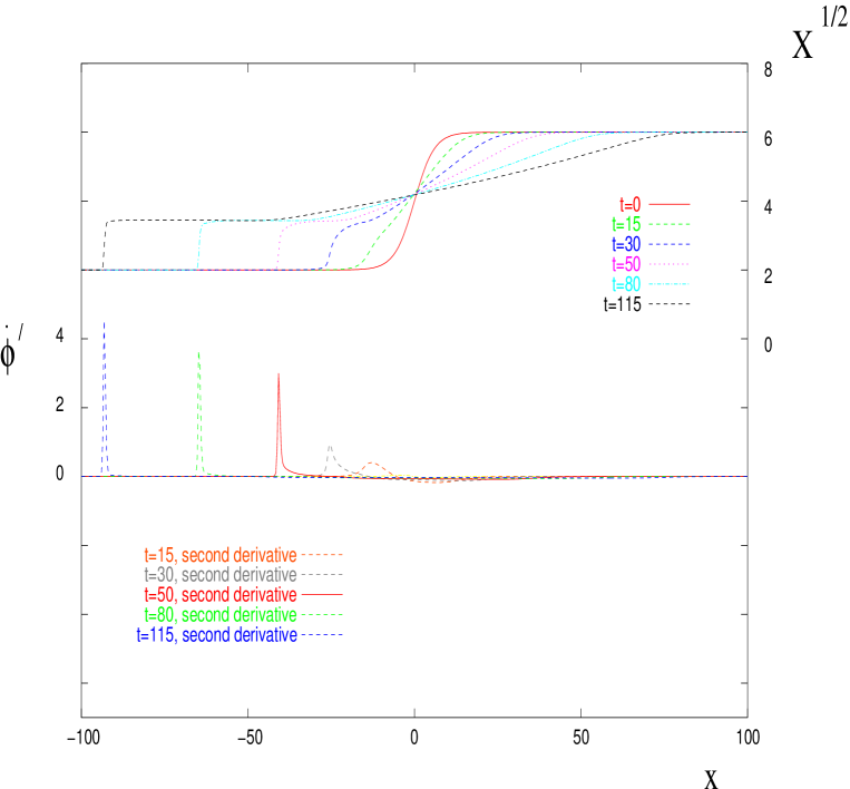
Figure 7: (1+1)-dimensional system. Profiles of $\sqrt{X}\equiv\sqrt{\dot{\phi}^{2}-\phi^{\prime 2}}$ (upper part) and $\dot{\phi}^{\prime}$ are shown at different times. Scales of $x$ and $t$ are arbitrary.

III.1.4 Around the critical point

Let us now consider another initial configuration, again with $\phi_{,x}=0$ but with the profile of $\phi_{,t}$ shown in fig. 8. This configuration corresponds to the region $r\lesssim a$ in fig. 2, i.e., the region near the point where $\phi_{,t}=c_{*}$ (in fig. 8 the bubble is meant to be on the left, like in fig. 2, and unlike in fig. 3). At the left of the critical point $\phi_{,t}=c_{*}$ the system is unstable. Let us study whether this instability propagates into the region on the right of this critical point, and also study the motion of this critical point as time evolves.

Figure 8: Initial data in the interior of a bubble.

Let us consider the behavior of the solution $\phi(x,t)$ in the region where $X\geq c_{*}^{2}$. In this region one can still use the variables $\rho$ and $\theta$ (or, equivalently, $\tau$ and $\theta$) in the Legendre conjugate problem. Now, the critical point $X\equiv\rho^{2}=c_{*}^{2}$ corresponds to $\tau=0$, and in the vicinity of this point the function $u(\tau,\theta)$ obeys eq. (30). ¿From the analogy to $O(2)$-symmetric $(2+1)$-dimensional problem it is clear that the solution and its derivatives never become singular at $\tau=0$, provided initial data are smooth. Futhermore, the solution is uniquely determined by the initial data at $X\geq c^{2}_{*}$. This means that the behavior of the solution $\phi(x,t)$ in the region $X\geq c^{2}_{*}$ is not sensitive to its behavour at $X<c^{2}_{*}$; the regions right of the critical point and left of the critical point do not talk to each other; whatever happens in the inner, tachyonic region of the bubble, has no effect on the outer region.

Let us see that the critical point $X=c^{2}_{*}$ moves left in fig. 8, i.e., inwards the bubble. To this end, we note that the initial data for the Legendre problem are again formulated in a finite interval of $\rho$, which is now $c_{*}\leq\rho<\rho_{+}$, i.e., in a finite interval $0<\tau<\tau_{+}$. The initial data is $u(\theta=0,\tau)=0$, while $u_{,\theta}(\theta=0,\tau)$ is singular at $\tau=\tau_{+}$. At non-zero $\theta$, the singularity propagates along the light-like line $\theta=\tau_{+}-\tau$, as shown in fig. 9. Near the singularity line the solution still has the form given by eq. (40), and this line again corresponds to $t\rightarrow\infty$. The slope (43) is positive on the lower right part of this line where $(\tau_{+}-\tau)$ is small, so the wave corresponding to the region near the corner $\theta=0$, $\tau=\tau_{+}$ is again moving right in fig. 8. This is now the motion outwards the bubble.

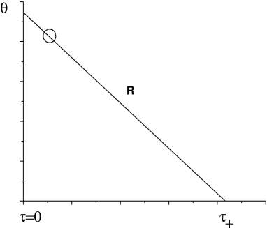
Figure 9: Singularity line in $(\tau,\theta)$-plane for initial data of fig. 8.

At $\rho$ close to $c_{*}$ one has $\rho\,\tau_{,\rho}=(\rho/c_{*}-1)^{-1/2}$, see eq.(29), which is large. Thus there is always a point denoted by a circle on the singularity line $R$, at which the slope (43) vanishes. Regions right and left of this point correspond to motion right and left in fig. 8, i.e. outwards and inwards the bubble, respectively. In particular, the critical point $\tau=0$ (i.e., $X=c_{*}^{2}$) moves left in fig. 8, i.e., inwards the bubble.

Another, direct way to see that the regions with $X<c_{*}^{2}$ and $X>c_{*}^{2}$ do not communicate with each other is to consider eq. (15) itself. Rescaling the field in such a way that

$$c_{*}=1$$

one has near the critical point

$$P^{\prime}=X-1$$

Equation (15) then reads

$$(3\phi_{,t}^{2}-\phi_{,x}^{2}-1)\phi_{,tt}-4\phi_{,x}\phi_{,t}\phi_{,xt}-(\phi_{,t}^{2}-3\phi_{,x}^{2}-1)\phi_{,xx}=0$$ (56)

This may be viewed as a wave equation with coefficients depending on $\phi_{,x}$ and $\phi_{,t}$. Let us find the characteristics of this equation that starts at a point $(x,t)$ where $X\equiv\phi_{,t}^{2}-\phi_{,x}^{2}=1$, i.e., at the critical point. At this point, eq. (56) reduces to

$$\phi_{,t}^{2}\phi_{,tt}-2\phi_{,x}\phi_{,t}\phi_{,xt}+\phi_{,x}^{2}\phi_{,xx}=0$$ (57)

Thus, the equation for the characteristics is

$$\phi_{,x}^{2}\cdot dt^{2}+2\phi_{,x}\phi_{,t}\cdot dxdt+\phi_{,t}^{2}\cdot dx^{2}=0$$

We see that the characteristics are degenerate and obey

$$\frac{dx}{dt}=-\frac{\phi_{,x}}{\phi_{,t}}$$ (58)

Let us now see that the critical point where $X=1$ moves precisely along this characteristic. The motion of the critical point is determined by the equation

$$d(\phi_{,t}^{2}-\phi_{,x}^{2}-1)\equiv(\phi_{,t}^{2}-\phi_{,x}^{2}-1)_{,t}dt+(\phi_{,t}^{2}-\phi_{,x}^{2}-1)_{,x}dx=0$$

which gives

$$\frac{dx}{dt}=-\frac{\phi_{,t}\phi_{,tt}-\phi_{,x}\phi_{,xt}}{\phi_{,t}\phi_{,xt}-\phi_{,x}\phi_{,xx}}$$

Making use of eq. (57) we find that the right hand side of this expression is precisely the same as the right hand side of eq. (58), so the charactristic and the world line of the point where $X=1$, indeed coincide.

Since the line $X=1$ is a characteristic, signals emitted on the left of this line do not propagate to the right of this line, and vice versa, i.e., the regions with $X<c_{*}^{2}$ and $X>c_{*}^{2}$ indeed evolve independently. Equation (58) determines the motion of the critical point; for an initial configuration shown in fig. 8 the velocity of this point initially vanishes (since $\phi_{,x}=0$ at $t=0$), and then becomes negative, as positive $\phi_{,x}$ develops. The critical point indeed moves inwards the bubble.

One way to understand the unusual property that the evolution in the regions with $X<c_{*}^{2}$ and $X>c_{*}^{2}$ proceeds independently, is to recall the expressions for the energy-momentum tensor and conserved current,

$$T_{\mu\nu} = 2P^{\prime}(X)\partial_{\mu}\phi\partial_{\nu}\phi-P(X)\eta_{\mu\nu}$$ (59)

$$j_{\mu} = P^{\prime}(X)\partial_{\mu}\phi$$ (60)

One observes that all components of $T_{\mu\nu}$ and $j_{\mu}$ are equal to zero at the surface in space where $X=c_{*}^{2}$. Thus, there is no transfer of energy and charge between the regions with $X<c_{*}^{2}$ and $X>c_{*}^{2}$. This explains, at least partially, the independence of the evolution in these two regions. It is worth stressing that this argument works in any number of dimensions.

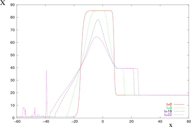
Figure 10: Initial stages of evolution of a bubble in $(1+1)$ dimensions. Profiles of $X$ are shown at different times. The irregular pattern at $x\lesssim-40$ for $t=22$ is due to instabilities in the tachyonic region where $X<c_{*}^{2}\equiv 1$.

III.1.5 Overall evolution

Combining the two pictures, corresponding to the initial data of figs. 3 and 8, we obtain the following qualitative properties of the evolution of a bubble, still in $(1+1)$ dimensions. The inner part of the bubble is unstable due to the tachyonic character of the region $c_{**}^{2}<X<c_{*}^{2}$. Nevertheless, the region $X\geq c_{*}^{2}$ is not sensitive to this instability. The critical point where $X=c_{*}^{2}$ moves towards the center of the bubble, so the region of large fields (hole in the ghost condensate) remains of small size. In the outer part, a wave moving outwards the bubble develops. Eventually this wave forms a kink. We show in fig. 10 the evolution of a bubble, which we obtained by solving eq. (15) numerically with the bubble-like initial data (in particular, initially $\phi_{,x}=0$). The region left of $x\approx-20$ in this figure (units of $x$ and $t$ are arbitrary) has initially $X<1$. The field at large negative $x$ is thus unstable; this instability is manifest in fig. 10. The motion of the boundary of the tachyonic region to the left (inwards the bubble) and a shock wave moving right are also clearly visible.

III.2 Four dimensions

Although the above analysis has been performed in $(1+1)$ dimensions, we argue that our main findings are valid in $(3+1)$-dimensional theory as well, at least for $O(3)$-symmetric bubbles. At large distances from the bubble center, the curvature of a sphere $r=\mbox{const}$ is small, so the evolution is similar to that in $(1+1)$-dimensional theory. There are two consequences of this simple observation. First, the tachyonic region, where $X<c_{*}^{2}$, does not expand; instead, it shrinks and forms a hole in the ghost condensate. The energy of this region is negative but finite at the moment of nucleation. According to eq. (59), there is no transfer of energy from the hole to the outer region where $X>c_{*}^{2}$, so the overall energy of the outer region, referenced from the energy of the original background $\dot{\phi}=c$, remains a finite constant.

Second, an outgoing wave of positive energy eventually forms a shock. It is conceivable that the UV effects smoothen out the profile of the wave. In front of the wave, i.e., at large $r$, the ghost field is still in its original state, $\vec{\nabla}\phi=0$, $\dot{\phi}=c$. Let us discuss the field behind the wave.

Let us first consider the special value of the original background, $\dot{\phi}=c_{*}$. In that case the conservation of energy requires that the background behind the outgoing wave is also $\dot{\phi}=c_{*}$, $\vec{\nabla}\phi=0$. This follows from the fact that the energy density of the original background is zero, while the overall energy of the positive energy region (outside the hole) is finite. This implies that $X=c_{*}^{2}$ behind the outgoing wave, otherwise the energy of the positive energy region would increase as $r^{3}(t)$ where $r(t)$ is the radius of the wave, which grows in time, $r(t)\to\infty$ as $t\to\infty$. The property that $X=c_{*}^{2}$ behind the wave, does not guarantee by itself that the background behind the wave is the same as the original background. However, the energy density of the wave decreases in time (otherwise its total energy would grow as $r^{2}(t)$). Therefore the amplitude of the wave decays, which is only possible if $\vec{\nabla}\phi=0$, $\dot{\phi}=c_{*}$ both in front of and behind the wave.

The above argument does not work for the general values of the original background, $\dot{\phi}=c>c_{*}$. In that case the conservation of energy and charge does not forbid that the energy density behind the outgoing wave be smaller than the energy density of the original background (i.e., of the field in front of the wave). However, in our numerical simulations the background behind the outgoing wave(s) always settled down to its original value, so the energy of the wave did not grow in time, and the amplitude of the wave decreased as it moved away from the bubble center.

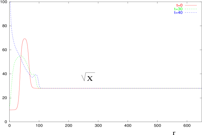
Figure 11: Initial stages of evolution of a bubble in $(3+1)$ dimensions. Profiles of $\sqrt{X}$ are shown at different times. Outgoing and incoming waves are formed, the incoming wave eventually bounces from the origin.

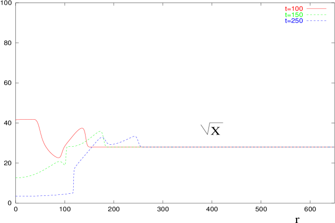
Figure 12: The second outgoing wave forms a kink. Note that the value of $X$ near the origin temporarily becomes smaller than in the original background.

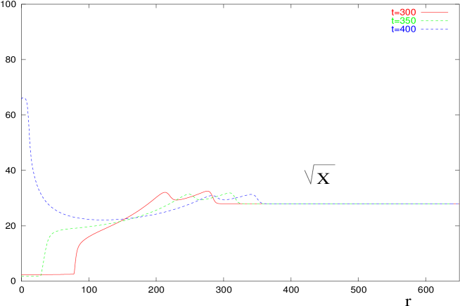
Figure 13: The second kink moves back and hits the origin.

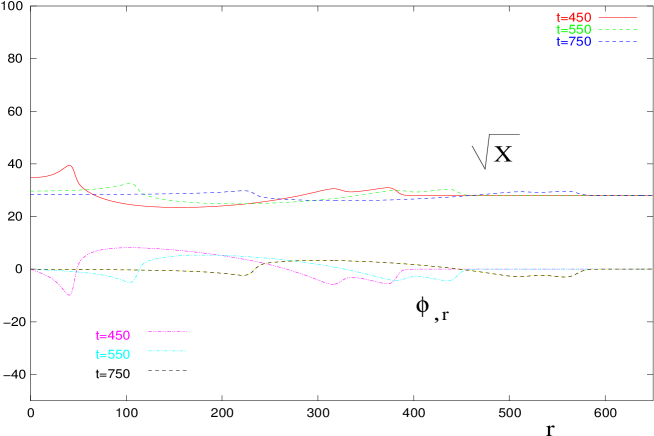
Figure 14: The third outgoing wave is formed; the background behind the outgoing waves settles down to its original value.

In numerical simulations, we observed a fairly complex behavior of the system even in the $O(3)$-symmetric case. As a reservation, we did not incorporate the region where $X<c_{*}^{2}$ into our numerical study of the long-time properties of the solutions. The reason is that the system is unstable for $X<c_{*}^{2}$, and this instability becomes intolerable in numerical simulations too early. Instead, we considered initial data such that $\vec{\nabla}\phi=0$, $\dot{\phi}\geq c_{*}$. To mimic possible effects of the boundary of the stable region (a surface at which $X=c_{*}^{2}$), we considered various boundary conditions near the origin, namely (i) smoothness at the origin, $\phi_{,r}=0$ at $r=0$; (ii) free boundary condition at some fixed $r=r_{h}$ (meant to be the radius of the hole); (iii) $X\equiv\phi_{,t}^{2}-\phi_{,r}^{2}=c_{*}^{2}$ at $r=r_{h}$. The overall behavior of the solutions at $r\gg r_{h}$ was essentially independent of the choice of the boundary condition.

A typical sphericaly symmetric solution in the theory with the potential (2) is shown in figs. 11 – 14. The initial data for this solution are such that $\phi_{,r}=0$ while $\dot{\phi}$ has the bubble-like shape, as shown in fig. 11. The initial stages of the evolution, shown in figs. 11 – 13, are indeed quite complex, but at late times the solution is simple: there is a sequence of outgoing waves with the backgrond behind them equal to the background in front, see fig. 14. The amplitudes of the outgoing waves indeed decrease in time, so the system settles down back to the homogeneous configuration $\phi_{,r}=0$, $\dot{\phi}=c$.

Thus, the outcome of the entire process discussed in this paper is a hole in ghost condensate plus a few outgoing “ghost waves” (in quantum theory the latter are particles of the ghost field $\phi$). Without knowing the UV-complete theory one cannot tell much about the properties of the negative energy holes. Our analysis implies that these holes do not expand, and thus remain of microscopic size. Although in the theory with the action (1) per se the field inside the hole is unstable, it is conceivable that the state of the hole gets stabilized due to UV effects. It is of interest to further investigate the phenomenology of ghost condensate with holes.

The authors are indebted to N. Arkani-Hamed, F. Bezrukov, S. Dubovsky, D. Gorbunov, A. Gorsky, D. Levkov, M. Libanov, M. Luty and S. Sibiryakov for stimulating discussions. This work was supported in part by RFBR grant 02-02-17398, CRDF award RP-1-2364-MO-02 and US-DOE grant DE-FG02-91ER40676. D.K. acknowledges the support by Dynasty Foundation.

References

-
(1)
C. Charmousis, R. Gregory and V. A. Rubakov,
Phys. Rev. D 62 (2000) 067505
[arXiv:hep-th/9912160];
R. Gregory, V. A. Rubakov and S. M. Sibiryakov, Phys. Rev. Lett. 84 (2000) 5928 [arXiv:hep-th/0002072]. - (2) I. I. Kogan, S. Mouslopoulos, A. Papazoglou, G. G. Ross and J. Santiago, Nucl. Phys. B 584 (2000) 313 [arXiv:hep-ph/9912552].
- (3) G. R. Dvali, G. Gabadadze and M. Porrati, Phys. Lett. B 485 (2000) 208 [arXiv:hep-th/0005016].
- (4) T. Jacobson and D. Mattingly, Phys. Rev. D 64, 024028 (2001).
- (5) K. Freese and M. Lewis, Phys. Lett. B 540, 1 (2002) [arXiv:astro-ph/0201229].
- (6) S. M. Carroll, V. Duvvuri, M. Trodden and M. S. Turner, arXiv:astro-ph/0306438.
- (7) N. Arkani-Hamed, H. C. Cheng, M. A. Luty and S. Mukohyama, arXiv:hep-th/0312099.
- (8) B. Holdom, arXiv:hep-th/0404109.
- (9) C. Armendariz-Picon, V. Mukhanov and P. J. Steinhardt, Phys. Rev. Lett. 85, 4438 (2000) [arXiv:astro-ph/0004134]. C. Armendariz-Picon, V. Mukhanov and P. J. Steinhardt, Phys. Rev. D 63, 103510 (2001) [arXiv:astro-ph/0006373].
- (10) S. L. Dubovsky, arXiv:hep-ph/0403308.
- (11) M. Peloso and L. Sorbo, arXiv:hep-th/0404005.
- (12) A. V. Frolov, arXiv:hep-th/0404216.
- (13) I. Y. Kobzarev, L. B. Okun and M. B. Voloshin, Sov. J. Nucl. Phys. 20, 644 (1975) [Yad. Fiz. 20, 1229 (1974)].
- (14) S. R. Coleman, Phys. Rev. D 15, 2929 (1977) [Erratum-ibid. D 16, 1248 (1977)].
- (15) G. N. Felder, L. Kofman and A. Starobinsky, JHEP 0209, 026 (2002) [arXiv:hep-th/0208019].
- (16) G. W. Gibbons, arXiv:hep-th/0302199.
- (17) K. M. Lee, Phys. Rev. Lett. 61, 263 (1988).
- (18) S. R. Coleman and K. M. Lee, Nucl. Phys. B 329, 387 (1990).