Multi-leg calculations with the GRACE/1-LOOP system
— Toward Radiative Corrections to $e^{+}e^{-}\rightarrow\mu^{-}\overline{\nu}u\overline{d}$ —

Abstract

We performed the calculation of the full $O(\alpha)$ corrections to $e^{+}e^{-}\rightarrow\mu^{-}\overline{\nu}u\overline{d}$ with the help of the GRACE/1-LOOP system. We discuss how a finite decay width introduces a serious gauge invariance breaking, particularly for infrared 5-point functions. This is related to the way the reduction of those functions is performed and to the treatment of the width in the reduction.

KEK–CP–154
LAPTH–1053

1 Introduction

The first calculation of the full $O(\alpha)$ corrections to $e^{+}e^{-}\rightarrow\nu\overline{\nu}H$ was presented at the RADCOR/L&L 2002 workshop[1]. Since then, several authors published the radiative corrections to several important $2\rightarrow 3$ processes: $e^{+}e^{-}\rightarrow\nu\overline{\nu}H$[2, 3, 4, 5], $e^{+}e^{-}\rightarrow t\overline{t}H$[6, 7, 8, 9], $e^{+}e^{-}\rightarrow ZHH$[10, 11], $\gamma\gamma\rightarrow t\overline{t}H$[12], $e^{+}e^{-}\rightarrow e^{+}e^{-}H$[13], and $e^{+}e^{-}\rightarrow\nu\overline{\nu}\gamma$[13]. Now, full EW 1-loop calculations are well under control for $2\rightarrow 3$ processes in the SM. In this paper, we discuss the case for a $2\rightarrow 4$ process.

As a first trial we take a typical LEP-2 process $e^{+}e^{-}\rightarrow\mu^{-}\overline{\nu}u\overline{d}$. Although a status report on a similar attempt has appeared[14], there still is no complete result.

2 Motivation

For LEP2 experiments, the Double Pole Approximation(DPA)[15] and the fermion loop scheme[15] were used to predict the cross sections for $e^{+}e^{-}\rightarrow$ 4-fermions. They have the following features:(1) Gauge invariance is guaranteed. (2) It was sensible to split all 10 tree diagrams(CC10) into the doubly resonant ones(CC03) and others. The constant width is introduced in a naive way. In the energy region at the future linear-collider, however, non-CC03 diagrams are not negligible. For example, at $\sqrt{s}=500$ GeV, the tree level cross sections for CC03 and CC10 are 213.56 fb and 222.39 fb, respectively. The difference between them reaches 4%. Therefore, the size of the radiative corrections to CC10 should be carefully estimated at the TeV energy region.

3 Structure of the calculations

GRACE/1-LOOP[16] has been used for the calculation which proceeds through the following steps: 1) Evaluation of the numerators, for which the symbolic manipulation system is used. In order to shorten the size of the matrix elements, the fermion masses $m_{e},m_{\mu}$, $m_{u},m_{d}$ are neglected when integrating over phase space. 2) Evaluation of the loop integrals. After 5- and 6-point integrals are reduced to 4-point functions, FF[17] and other analytic formulas are invoked for 4-, 3-and 2-point integrals. All masses are kept in the loop integrals. 3) Construction of kinematics. Here masses are also kept exactly.

4 The reduction algorithm of $N(\geq 5)$ point functions

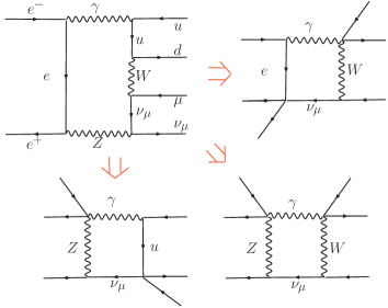
Figure 1: Example of unstable 4-point functions obtained in the reduction of a 6-point function

The amplitude with 5-point function[18, 3, 10] is

$$T^{(5)} \propto \int\frac{d^{n}l}{(2\pi)^{n}i}\frac{l_{\mu}l_{\nu}\cdots l_{\rho}}{D_{0}D_{1}\cdots D_{4}},$$ (1)

where $D_{0}=l^{2}-m_{0}^{2}$ and $D_{i}=(l+s_{i})^{2}-m_{i}^{2},i=1,\cdots,4$ and $s_{i}$ is a combination of external momenta.

Multiplying the identities

$$g^{\mu\nu}=\sum_{i,j=1}^{4}s_{i}^{\mu}(A^{-1})_{ij}s_{j}^{\nu},$$

with the loop momentum $l$,

$$l^{\mu} = \sum_{i,j}s_{i}^{\mu}(A^{-1})_{ij}(l\cdot s_{j}),$$ (2)

$$= \frac{1}{2}\sum_{i,j}(A^{-1})_{ij}(D_{j}-D_{0}-\Delta_{j})s_{i}^{\mu},$$

where $A_{ij}=s_{i}\cdot s_{j}$ and $\Delta_{i}=s_{i}^{2}-m_{i}^{2}$, we can reduce the numerator to

$$l_{\mu}l_{\nu}\cdots l_{\rho}=\frac{1}{2}\sum_{i,j}(A^{-1})_{ij}(D_{i}-D_{0}-\Delta_{i})s_{j}^{\mu}l_{\nu}\cdots l_{\rho}.$$ (3)

This method is also applicable for the reduction of a 6-point function to a sum of 4-point functions. There is also a standard reduction method where the following identity is used;

$$l^{2}=\sum_{i,j}(l\cdot s_{i})A_{ij}(l\cdot s_{j}).$$ (4)

Because this method not only raises the rank of the momentum tensor in the numerator but makes the resultant source codes very lengthy compared with Eq.3, GRACE/1-LOOP uses this identity only as an option. As mentioned the system employs the FF package for the evaluation of 4-point functions. It happens, however, that this package leads to numerical instabilities or inconsistency in some cases having to do with some infra-red boxes. This occurs for instance when an internal massless particle is involved in some non-IR boxes like those obtained from a 6-point function as shown in Fig.1. Some infra-red boxes also need to be regulated by the introduction of a width for the particle($W$ or $Z$) circulating in the loop. We implement a constant fixed width for such cases. For all these particular cases we use special in-house routines. For the computations we performed till now these routines have worked quite well for any $2\rightarrow 2$ and all $2\rightarrow 3$ one-loop processes. However, for the problem at hand, we have met a difficulty in carrying out the evaluation of a $5$-point function when the $W$ width is required.

Table 1: Stability of the matrix element squared, Eq. 5, against the changes of $C_{UV}$ and $\lambda$.

graph	$C_{UV}$	$\lambda=10^{-18}$ GeV	$\lambda=10^{-21}$ GeV
full	0	-0.85388129300841993023002220162E-03	-0.85388129300794622839025322460E-03
full	100	-0.85388129300841993023002220166E-03	-0.85388129300794622839025322465E-03
prod.	0	-0.85388086448063959950419248157E-03	-0.85388086990548652947683563335E-03
prod.	100	-0.85388086452253511266116024563E-03	-0.85388086994738204263380339741E-03

5 1-loop diagrams for $e^{+}e^{-}\rightarrow\mu^{-}\overline{\nu}u\overline{d}$

We introduce two sets of diagrams, the full set and the production set. In the standard model and within the non-linear gauge fixing conditions[19], one counts 44 tree-level and 6094 1-loop diagrams. This defines the full set.

When the masses of the electron, $\mu$, $u$- and $d$-quark are ignored in the numerator of the matrix elements, we obtain the production set which consists of 10 tree diagrams(CC10) and 668 1-loop diagrams (with 88 pentagon and 60 hexagon graphs).

6 Check of codes

The following set of input parameters are used in the calculation: Throughout this paper, the results are expressed in terms of the fine structure constant in the Thomson limit $\alpha_{QED}^{-1}=137.0359895$ and the $Z$ mass $M_{Z}=91.1876$GeV. The on-shell renormalization scheme uses $M_{W}$ as an input parameter. Nevertheless the numerical value of $M_{W}$ is derived through $\Delta r$[20]. $M_{W}$ thus changes as a function of $M_{H}$. We take $m_{u}=m_{d}=63$ MeV, $m_{s}=92$ MeV, $m_{c}=1.5$ GeV, $m_{b}$=4.7GeV. This set of masses gives a “perturbative” value of $\alpha(M_{Z})$ compatible with the current value derived experimentally. We also take $m_{top}$=180GeV. With these values, we find $M_{W}$ =80.4163 and $\Gamma_{Z}$=2.4952GeV for $M_{H}$=120GeV. $\Gamma_{W}$=2.118GeV is taken from PDG.

The results of the calculation are checked by performing four kinds of tests at few points in phase space. For this we worked with the full set of diagrams in quadruple precision. The first check is the ultraviolet finiteness test. The regulator constant $C_{UV}=1/\varepsilon-\gamma_{E}+\log 4\pi,n=4-2\varepsilon$ is kept in the matrix elements. In varying this parameter $C_{UV}$, we found that the result is stable with an accuracy reaching $29$ digits. Infrared(IR) finiteness is also checked by introducing a fictitious photon mass $\lambda$, treated as an input parameter in the code. The sum of loop and bremsstrahlung contributions stays stable against variations in $\lambda$ with an accuracy of $12$ digits. Table 1 shows the stability for both cases of full set and production set(prod.). For the latter the accuracy worsens to order $O(m_{\mu}^{2}/s)$ because the masses of the fermions are neglected in the numerator.

The third check relates to the independence on the parameter $k_{c}$ which is a soft photon cut parameter that separates soft photon radiation(analytical formula) and the hard photon performed by the Monte-Carlo integration. Gauge parameter independence of the result is performed as the last check through a set of five gauge fixing parameters. For the latter a generalized non-linear gauge fixing condition[19] has been chosen. In total the amplitude contains 5 free parameters: $\tilde{\alpha},\tilde{\beta},\tilde{\delta},\tilde{\varepsilon}$ and $\tilde{\kappa}$. In this check we set $\Gamma_{W}=\Gamma_{Z}=0$ and keep all masses in the numerator. The whole matrix element shows no dependence on any of the gauge parameters in more than 21 digits.

Table 2: Cancellation between each 4-point function in Eq.(8) at a phase point with the matrix elements of Fig.2

box	$\Gamma_{W}=0$	$\Gamma_{W}\neq 0$
	(real, imag)	(real, imag)
1	( $-17.69217505$,    66.88369265)	(   $-4.22744975$,   2.9465712570)
2	($-929.96695924$,  1372.81890328)	( $-120.36833308$,  39.2204483424)
3	( 782.70500402, -5690.37576950)	(  321.80994609, $-283.271079293$)
4	( 410.83071602,  4557.14502347)	( $-199.63435655$,  275.873356743)
5	($-245.31384970$,  -301.36098220)	(    0.65534291,  $-27.683645798$)
sum	(   0.56273604,     5.11086770)	(   $-1.76485038$,    7.085651250)

Figure 2: An IR 5-point function and a tree diagram.

7 Status of calculation

All the calculations were done in quadruple precision. When we sampled points in phase space to carry out the MC integration, we encountered an unstability with IR 5-point diagrams. In Fig.2 we show such an example with a product of a 1-loop IR diagram and a tree diagram. It is to be noted that the 1-loop graph is obtained from the tree by adding a photon that joins $e^{-}$ and $u$. A 5-point diagram is written as a sum of five 4-point integrals. For the product of the two diagrams (the labelling is assigned automatically by the system), we then write

$$[\hbox{IR-loop}]^{(5)}\equiv 2T_{5245}T_{41}^{\dagger}$$ (5)

$$= I^{(4)IR}_{1}+I^{(4)IR}_{2}+I^{(4)}_{3}+I^{(4)}_{4}+I^{(4)}_{5},$$

which contains two infrared divergent boxes. Currently the widths $\Gamma_{W}$ and $\Gamma_{Z}$ are retained only in the IR part of the box integrals in such a way

$$I^{(4)IR}_{1}\sim{1\over D_{W}(q^{2})}\left[\log{\lambda\sqrt{\tilde{M}_{W}^{2}}\over D_{W}(q^{2})}\log(\cdots)+\cdots\right],$$ (6)

$$D_{W}(q^{2}) \equiv q^{2}-\tilde{M}_{W}^{2}=q^{2}-M_{W}^{2}+i\Gamma_{W}M_{W}$$

and also in the reduction formulas for 4-points. Without the width, 3 digits cancellation is observed among the boxes, as shown in Table 2 at some phase space point near the $W$-pole,

$$(q^{2}-M_{W}^{2}+i\Gamma_{W}M_{W})_{ud}$$

$$=-169.3611+167.1833i\qquad({{\rm GeV}}^{2})$$ (7)

On the other hand, when $\Gamma_{W}\neq 0$, Table 2 shows less cancellation. This led to a bad convergence of the phase space integration as we will clearly demonstrate below. Though the mechanism for this cancellation with zero width is not fully understood now, it is highly probable that an identity including

$$\{(l.p_{1})\varepsilon(p_{2},p_{3},p_{4},p_{5})-(l.p_{2})\varepsilon(p_{1},p_{3},p_{4},p_{5})$$

$$+(l.p_{3})\varepsilon(p_{1},p_{2},p_{4},p_{5})-(l.p_{4})\varepsilon(p_{1},p_{2},p_{3},p_{5})$$

$$+(l.p_{5})\varepsilon(p_{1},p_{2},p_{3},p_{4})\}\times(l.p_{6})=0$$

causes the trouble. This identity relates the five box integrals among each other. No such phenomenon took place for 6-point diagrams nor non-IR 5-points. Also we did not encounter such difficulty in all $2\to 3$ processes we studied till now. The number of independent fermion lines may be related to this undesirable situation. As mentioned above, GRACE/1-LOOP adopts Eq.3 for the reduction. We found, however, that when we used Eq.4 no such problem happened.

8 Test run of integration

In order to confirm that an improper treatment of the width in the infrared divergent 5-point function is the cause of bad convergence, we temporarily took the following ad hoc regularization in the loop amplitude

$$\sigma^{(5)}=2\Re\left(T_{\hbox{IR-loop}^{(5)}}T_{\hbox{tree}}^{\dagger}\right)$$

$$\Longrightarrow 2\Re\left[{q^{2}-M_{W}^{2}\over q^{2}-\tilde{M}_{W}^{2}}\left(T_{\hbox{IR-loop}^{(5)}}\right)_{\Gamma_{W}=0}T_{\hbox{tree}}^{\dagger}\right]$$

(8)

and integrated all the diagrams in the phase space. The integration is carried out by BASES. Those diagrams which contribute less than 0.01 fb were omitted to leave 361 1-loop diagrams. Hard photon emission is also included.

At $\sqrt{s}=500~{}{\rm GeV}$, $\sigma_{tree}=222.39\pm 0.01$fb. Table 3 shows the results of the integrated cross section for each set of $n$-point diagrams with 50,000 sampling points, together with their MC error. The column “original(IR)” shows the results of the diagrams related to the infrared divergence as extracted normally through Eqs. 5-6 or an equivalent form for the other $n-$point IR diagrams. On the other hand “ad hoc(IR)” is the result after making the modification in Eq.8 for the same sets of diagrams as “original(IR)”. The last column contains those diagrams which do not have any infrared divergence. For the case of 5-point functions of the type “original(IR)”, the integrated error is extremely huge due to the mismatch between its corresponding 4-point parts as mentioned earlier. After applying Eq.8, there is a drastic improvement in the error and the central value of the integration is also shifted. Other contributions from $n$-point functions remain the same within the integration error if one applies the “ad hoc” prescription. Table 3 suggests that a proper treatment of the width in 5-point functions is crucial to improve the situation but one still needs to find a proper justification for the factorization.

Table 3

Integrated cross sections in fb showing the contribution of each set of $n$-point diagrams for the test run. The parentheses show the MC integration error.

graph	original(IR)	ad hoc(IR)	non-IR
6-pnt	-921(  16)	-914( 6)	small
5-pnt	-4221(2224)	+2729(17)	-80(10)
4-pnt	-4041(  26)	-3999(26)	+216(7)
3-pnt	+735(   6)	+735( 6)	-258(2)
2-pnt			-27(0.3)
self	-104(   2)	-104( 2)	-9(0.08)
cnt	+305(  26)	+305(26)	small
soft	+990( 8)
hard			+461(0.5)
total	-7257(2223)	-258( 9)	+302(9)

9 Summary

One-loop amplitudes of the full $6094$ diagrams for $e^{+}e^{-}\rightarrow\mu^{-}\overline{\nu}u\overline{d}$ were generated by the GRACE/1-LOOP system. Non-linear gauge invariance has shown the consistency of the full set of amplitudes and the system itself. A new reduction algorithm from a 6-point function to 4-point function works well. A finite decay width brings a serious breaking of gauge invariance, particularly for 5-point infrared integrals. It is clear now that the radiative corrections to $2\to 4$ processes are calculable, though more improvements are inevitable.

10 Acknowledgment

This work is part of a collaboration between the Minami-Tateya group and LAPP/LAPTH. D. Perret-Gallix and G. Bélanger deserve special thanks for their contribution. The author(J.F.) also would like to acknowledge the local organizing committee of LOOPS/LEGS 2004 for a stimulating workshop and for their nice organization. This work was supported in part by Japan Society for Promotion of Science under the Grant-in-Aid for scientific Research B(no. 14340081) and GDRI of the French National Centre for Scientific Research (CNRS).

References

- [1] G. Bélanger et.al, Nucl. Phys. B116(Proc. suppl.) (2003)353.
- [2] F. Jegerlehner and O. V. Tarasov, Nucl. Phys. B116(Proc. suppl.) (2003)83.
- [3] G. Bélanger, F. Boudjema, J. Fujimoto, T. Ishikawa, T. Kaneko, K. Kato and Y. Shimizu, Phys. Lett. B 559(2003)252.
- [4] A. Denner, S. Dittmaier, M. Roth and M. M. Weber, Phys. Lett. B 560(2003)196.
- [5] A. Denner, S. Dittmaier, M. Roth and M. M. Weber, Nucl. Phys. B660(2003)289.
- [6] You Yu, Ma Wen-Gan, Chen Hui, Zhang Ren-You, Sun Yan-Bin and Hou Hong-Sheng, Phys. Lett. B 571(2003)85.
- [7] G. Bélanger, F. Boudjema, J. Fujimoto, T. Ishikawa, T. Kaneko, K. Kato, Y. Shimizu and Y. Yasui, Phys. Lett. B 571(2003)163.
- [8] A. Denner, S. Dittmaier, M. Roth and M. M. Weber, Phys. Lett. B 575(2003)290.
- [9] A. Denner, S. Dittmaier, M. Roth and M. M. Weber, Nucl. Phys. B680(2004)85.
- [10] G. Bélanger, F. Boudjema, J. Fujimoto, T. Ishikawa, T. Kaneko, K. Kato and Y. Shimizu, Phys. Lett. B 576(2003)152.
- [11] Zhang Ren-You, Ma Wen-Gan, Chen Hui, Sun Yan-Bin and Hou Hong-Sheng, Phys. Lett. B 578(2004)349.
- [12] Chen Hui, Ma Wen-Gan, Zhang Ren-You, Zhou Pei-Jun, Hou Hong-Sheng and Sun Yan-Bin, Nucl. Phys. B683(2004)196.
- [13] F. Boudjema et.al.,hep-ph/0404098 and hep-ph/0407065.
- [14] A. Vicini, talk at ”LoopFest at BNL”(May 2002).
- [15] see M.W. Grünewald et.al. in Reports of the Working Group on Precision Calculations for LEP2 Physics, eds. S. Jadach, G. Passarino and R. Pittau(CERN2000-009, Geneva, 2000), 1 and references are therein.
- [16] G. Bélanger et.al, hep-ph/0308080.
- [17] G.J. van Oldenborgh, Z. Phys. C46(1990)425.
- [18] A. Denner and S. Dittmaier, Nucl. Phys. B658(2003)175.
- [19] F. Boudjema and E. Chopin, Z. Phys. C73(1996)85.
- [20] Z. Hioki, Acta. Phys. Polon. B27(1996)2573.