Abstract

The shape of the electron energy spectrum in ³H $\beta$-decay permits a direct assay of the absolute scale of the neutrino mass; a highly accurate theoretical description of the electron energy spectrum is necessary to the empirical task. We update Sirlin’s calculation of the outer radiative correction to nuclear $\beta$-decay to take into account the non-zero energy resolution of the electron detector. In previous ³H $\beta$-decay studies the outer radiative corrections were neglected all together; only Coulomb corrections to the spectrum were included. This neglect artificially pushes $m_{\nu}^{2}<0$ in a potentially significant way. We present a computation of the theoretical spectrum appropriate to the extraction of the neutrino mass in the sub-eV regime.

Empirical evidence of neutrino oscillations in atmospheric, solar, and reactor neutrino data [2, 3, 4] compels the existence of non-zero neutrino masses, yet such experiments are insensitive to the absolute scale of a neutrino mass, for the oscillation experiments determine $\Delta m_{ij}^{2}\equiv m_{i}^{2}-m_{j}^{2}$, where $m_{i}$ is the mass of neutrino $i$. To determine the absolute value of the neutrino mass requires different methods. Cosmological constraints on the neutrino mass do exist [5], though our focus shall be on the study of the electron energy spectrum in tritium $\beta$-decay near its endpoint, as this represents the most sensitive terrestrial measurement. The spectrum shape constrains the mass of the neutrino, be it of Dirac or Majorana character, and the inferred mass is insensitive to phases in the neutrino mixing matrix — in contradistinction to the constraint on the neutrino mass from neutrinoless double $\beta$-decay. An accurate theoretical description of the expected electron energy spectrum is crucial to the determination of the neutrino mass; this demand grows as the sensitivity of the experiments increase. Indeed, future studies expect to probe the neutrino mass at the sub-eV level [6]. It is our purpose to realize a theoretical form of the requisite accuracy, though we shall begin by describing the form used in earlier tritium experiments.

With an anti-electron neutrino of mass $m_{\nu}$, neglecting neutrino mixing for simplicity, the Fermi form of the electron energy spectrum for tritium $\beta$-decay is [7]

$$\frac{d\Gamma_{F}}{dE_{e}}=\frac{G_{F}^{2}}{2\pi^{3}}|{\cal M}|^{2}F(Z,R_{\rm e},E_{e})p_{e}E_{e}(E_{e}^{\rm max}-E_{e})\sqrt{(E_{e}^{\rm max}-E_{e})^{2}-m_{\nu}^{2}}\,,$$ (1)

where $G_{F}$ is the Fermi constant, $p_{e}$, $E_{e}$, and $E_{e}^{\rm max}$ are the momentum, energy, and maximum endpoint energy, respectively, of the electron, and $|{\cal M}|^{2}$ is the absolute square of the nuclear matrix element, with $|{\cal M}|^{2}\sim 5.3$. A form of this ilk has been used to bound $m_{\nu}$ in previous experimental analyses of molecular tritium $\beta$-decay [8, 9, 10, 11, 12, 13, 14, 15]. Following the usual practice, we include a non-zero neutrino mass in the phase space contribution only. We set $\hbar=c=1$ throughout. The Fermi function, $F(Z,R_{\rm e},E_{e})$, captures the correction due to the Coulomb interactions of the electron with the charge $Ze$ of the daughter nucleus [16]. We adopt the usual expression [17], derived from the solutions of the Dirac equation for the point-nucleus potential $-Z\alpha/r$ evaluated at the nuclear radius $R_{\rm e}$ [18]; it differs from unity by a contribution of ${\cal O}(\alpha)$. The Fermi function includes the dominant electromagnetic effect, though an accurate extraction, or bound, of the neutrino mass does demand the inclusion of the remaining ${\cal O}(\alpha)$ correction. We shall demonstrate this point explicitly. This last effect, termed the radiative correction, is conventionally separated into an “inner” piece $\Delta_{R}$, which is absorbed in $|{\cal M}|^{2}$, as it is energy independent and thus of no consequence to our current study, and an “outer” piece $\delta_{R}$ [19]. The outer radiative correction applied in $\beta$-decay studies is due to Sirlin [19]:

$$\frac{d\Gamma}{dE_{e}}=\frac{d\Gamma_{0}}{dE_{e}}\left(1+\frac{\alpha}{2\pi}g_{S}(E_{e},E_{e}^{\rm max})\right)\,,$$ (2)

where $d\Gamma_{0}/dE_{e}=G_{F}^{2}|{\cal M}|^{2}p_{e}E_{e}(E_{e}^{\rm max}-E_{e})^{2}/(2\pi^{3})$, and, noting $\beta=p_{e}/E_{e}$,

$$g_{S}(E_{e},E_{e}^{\rm max}) = 3\ln\left(\frac{M}{m_{e}}\right)-\frac{3}{4}+4\left[\frac{\tanh^{-1}\beta}{\beta}-1\right]\left[\frac{(E_{e}^{\rm max}-E_{e})}{3E_{e}}-\frac{3}{2}+\ln\Big{\{}\frac{2(E_{e}^{\rm max}-E_{e})}{m_{e}}\Big{\}}\right]$$ (3)

$$+\frac{4}{\beta}L\left(\frac{2\beta}{1+\beta}\right)+\frac{\tanh^{-1}\beta}{\beta}\left[2(1+\beta^{2})+\frac{(E_{e}^{\rm max}-E_{e})^{2}}{6E_{e}^{2}}-4\tanh^{-1}\beta\right]\,,$$

with $M$ and $m_{e}$ the proton and electron mass, respectively, and $L(x)$ the Spence function. As in Ref. [19], we neglect terms of relative order $\alpha(E_{e}/M)\ln(M/E_{e})$, $\alpha E_{e}/M$, and smaller, throughout. The total ${\cal O}(\alpha)$ correction is given by $F(Z,R_{\rm e},E_{e})-1+(\alpha/2\pi)g_{S}(E_{e},E_{e}^{\rm max})$. Note that $\delta_{R}$ results from averaging $(\alpha/2\pi)g_{S}(E_{e},E_{e}^{\rm max})$ over the electron energy spectrum. To assess the relative sizes of $F$ and $g_{S}$, we note that in the endpoint region of tritium $\beta$-decay, for $E_{e}-m_{e}=18.5$ keV, e.g., $F\sim 1.19$, whereas $(\alpha/2\pi)g_{S}\sim 0.02$.

Since the absolute neutrino mass scale is inferred through the shape of the electron energy spectrum in the endpoint region, it is crucial to predict the shape of the theoretical spectrum with high accuracy. To this end, we update the calculation of Ref. [19] to take the energy resolution of the electron detector into account. To understand the significance of this, we recall that Sirlin’s function contains not only virtual photon corrections to the $\beta$-decay process but also bremsstrahlung contributions, to yield an additional real photon in the final state. Only their sum is infrared finite; the infrared divergence in each contribution is regulated by giving the photon a small mass $\lambda$, with the $\lambda\to 0$ limit to be taken after the sum has been computed and the infrared divergent pieces cancelled. The finite portion of the bremsstrahlung contribution is sensitive to the precise manner in which the experiment is effected. In Sirlin’s function the energy resolution of the electron detector is implicitly assumed to be zero; that is, the $e^{-}$ and $\gamma$ are always distinguishable. A consequence of this is that Eq. (3) contains a logarithmic divergence as $E_{e}\to E_{e}^{\rm max}$. This singularity can be removed by including soft photon contributions to all orders in perturbation theory [20]; however, it can also be removed by taking the energy resolution of the detector into account, as we consider here. The bremsstrahlung contribution comes from integrating the photon energy over its entire kinematic range, namely

$$\frac{\alpha}{2\pi}\left(\frac{d\Gamma_{0}}{dE_{e}}\right)g_{S,b}(E_{e},E_{e}^{\rm max})=\int_{\lambda}^{E_{e}^{\rm max}-E_{e}}dE_{\gamma}\left(\frac{d^{2}\Gamma_{\gamma}(E_{e},E_{\gamma})}{dE_{e}dE_{\gamma}}\right)\,,$$ (4)

where $d^{2}\Gamma_{\gamma}(E_{e},E_{\gamma})/dE_{e}dE_{\gamma}$ is the doubly differential decay rate for the radiative $\beta$-decay process. Nevertheless, the detector energy resolution $\Delta E$ can, in principle, influence the shape of the electron energy spectrum. That is, for $E_{\gamma}\leq\Delta E$, the electron and photon cannot be distinguished; indeed, this is precisely why the bremsstrahlung contribution can enter to render an infrared-finite, ${\cal O}(\alpha)$ radiative correction to $\beta$-decay. In this event the detector records the sum of the electron and photon energies as the “electron” energy. For $E_{\gamma}>\Delta E$, however, the electron and photon energies are distinguishable, and their energies can be recorded separately. To separate the contributions we note that the total bremsstrahlung contribution to $\delta_{R}$ must be insensitive to such experimental details. In passing, we note related discussions of the impact of the detection threshold for bremsstrahlung photons in the radiative corrections to $\nu$ capture on deuterium [21, 22, 23, 24], as well as to $\nu-e$ scattering [25]. The bremsstrahlung contribution to the total outer radiative correction $\delta_{R}$ — we retain the photon mass $\lambda$ throughout — is

$$\tilde{\delta}_{R,b}=\int_{m_{e}}^{E_{e}^{\rm max}-\lambda}dE_{e}\int_{\lambda}^{E_{e}^{\rm max}-E_{e}}dE_{\gamma}\,f(E_{e},E_{\gamma})\,,$$ (5)

where $f(E_{e},E_{\gamma})\equiv d^{2}\Gamma_{\gamma}(E_{e},E_{\gamma})/dE_{e}dE_{\gamma}$. To find $\delta_{R}$ we must divide $\tilde{\delta}_{R,b}$ by a normalization factor $N$, determined by integrating Eq. (1) over the allowed phase space with $F=1$ and $m_{\nu}=0$. However, if the detector energy resolution is “infinite,” that is, if the electron detector always records ${\cal E}=E_{e}+E_{\gamma}$ [21], the total bremstrahlung contribution can be rewritten as

$$\tilde{\delta}_{R,b}=\int_{m_{e}+\lambda}^{E_{e}^{\rm max}}d{\cal E}\int_{\lambda}^{{\cal E}-m_{e}}dE_{\gamma}\,f({\cal E}-E_{\gamma},E_{\gamma})\,.$$ (6)

In both Eqs. (5) and (6), the integration over $E_{\gamma}$ yields the bremstrahlung correction to the electron energy spectrum. Although $\tilde{\delta}_{R,b}$ is universal, the shape correction to the electron energy spectrum is not. Let us now determine the shape correction for a finite energy resolution $\Delta E$. That is, for $E_{\gamma}\leq\Delta E$, ${\cal E}=E_{e}+E_{\gamma}$ is recorded, whereas for $E_{\gamma}>\Delta E$, $E_{e}$ is recorded. We can reorganize the total bremsstrahlung contribution in the following way:

$$\tilde{\delta}_{R,b} = \int_{m_{e}+\lambda}^{\Delta E+m_{e}}d{\cal E}\int_{\lambda}^{{\cal E}-m_{e}}dE_{\gamma}\,f({\cal E}-E_{\gamma},E_{\gamma})+\int_{\Delta E+m_{e}}^{E_{e}^{\rm max}}d{\cal E}\int_{\lambda}^{\Delta E}dE_{\gamma}\,f({\cal E}-E_{\gamma},E_{\gamma})$$ (7)

$$+\int_{m_{e}}^{E_{e}^{\rm max}-\Delta E}dE_{e}\int_{\Delta E}^{E_{e}^{\rm max}-E_{e}}dE_{\gamma}\,f(E_{e},E_{\gamma})\,.$$

Note that letting $\Delta E\to\lambda$ yields Eq. (5), whereas letting $\Delta E\to E_{e}^{\rm max}-m_{e}$ yields Eq. (6). If $\Delta E$ has a non-infinitesimal value, then infrared divergences are restricted to the first two terms — in the third, we may let $E_{\gamma}=\sqrt{k^{2}+\lambda^{2}}\to k$ with impunity. Thus we introduce

$$\frac{\alpha}{2\pi}\frac{d\Gamma_{0}}{d{\cal E}}{\cal I}_{\lambda}(k^{\rm max},{\cal E})=\int_{\lambda}^{k^{\rm max}}dE_{\gamma}\,f({\cal E}-E_{\gamma},E_{\gamma})\,$$

and

$$\frac{\alpha}{2\pi}\frac{d\Gamma_{0}}{dE_{e}}{\cal I}(\Delta E,E_{e})=\int_{\Delta E}^{E_{e}^{\rm max}-E_{e}}dE_{\gamma}\,f(E_{e},E_{\gamma})\to\int_{\Delta E}^{E_{e}^{\rm max}-E_{e}}dk\,f(E_{e},k)$$ (8)

to realize

$$g_{b}(\Delta E,E_{e},E_{e}^{\rm max}) = \Theta(\Delta E+m_{e}-E_{e}){\cal I}_{\lambda}(k^{\rm max}=E_{e}-m_{e},E_{e})$$ (9)

$$+ \Theta(E_{e}-(\Delta E+m_{e})){\cal I}_{\lambda}(k^{\rm max}=\Delta E,E_{e})$$

$$+ \Theta(E_{e}^{\rm max}-\Delta E-E_{e})){\cal I}(\Delta E,E_{e})\,.$$

With this, we determine that the radiative correction to the electron energy spectrum is

$$g(\Delta E,E_{e},E_{e}^{\rm max})=g_{b}(\Delta E,E_{e},E_{e}^{\rm max})+g_{v}(E_{e})\,,$$ (10)

where the virtual photon contribution $g_{v}\equiv 2{\cal A}-3/4$, with ${\cal A}$ as reported in Eq. (16) of Ref. [24]. To compute the integrals of Eq. (8) and thus $g_{b}(\Delta E,E_{e},E_{e}^{\rm max})$ we adapt the computation of radiative neutron $\beta$-decay in Ref. [26] to this case. In specific, we use the absolute squared matrix elements of Eqs. (13-16), and Eq. (20), dividing the latter by $8M^{2}$, in that work to determine $f(E_{e},E_{\gamma})$. In doing the integrals, we can neglect the recoil corrections to the phase space, so that $E_{\nu}=E_{e}^{\rm max}-E_{e}-k$. As a result, the dependence on the weak, hadron coupling constants is captured by $g_{V}^{2}+3g_{A}^{2}$, which we replace by $|{\cal M}|^{2}$; we also update the mass factors which appear as appropriate. We have verified that our computation of $g_{b}(\Delta E=0,E_{e},E_{e}^{\rm max})$ using this procedure and Eq. (5), in concert with $g_{v}$ of Ref. [24], yields Sirlin’s result [19], Eq. (3). For finite $\Delta E$ we find the following results:

$${\cal I}_{\lambda}(k^{\rm max},{\cal E})=6-4\left(1-\frac{\tanh^{-1}\beta_{\varepsilon}}{\beta_{\varepsilon}}\right)\ln\left(\frac{2k^{\rm max}}{\lambda}\right)+\frac{2\tanh^{-1}\beta_{\varepsilon}}{\beta_{\varepsilon}}+\frac{2}{\beta_{\varepsilon}}L\left(\frac{2\beta_{\varepsilon}}{1+\beta_{\varepsilon}}\right)$$

$$-\frac{2}{\beta_{\varepsilon}}(\tanh^{-1}\beta_{\varepsilon})^{2}+\frac{2}{\beta_{\varepsilon}}I_{k}^{-1}-\frac{2}{{\cal E}\beta_{\varepsilon}}I_{k}^{0}+\frac{1}{{\cal E}^{2}\beta_{\varepsilon}}I_{k}^{1}-4\frac{\sqrt{({\cal E}-k^{\rm max})^{2}-m_{e}^{2}}}{\sqrt{{\cal E}^{2}-m_{e}^{2}}}$$

$$+4\frac{1}{\beta_{\varepsilon}}\ln\left(\frac{{\cal E}-k^{\rm max}-\sqrt{({\cal E}-k^{\rm max})^{2}-m_{e}^{2}}}{{\cal E}-\sqrt{{\cal E}^{2}-m_{e}^{2}}}\right)$$

$$+4\ln\left(\frac{{\cal E}^{2}-m_{e}^{2}-{\cal E}k^{\rm max}+\sqrt{{\cal E}^{2}-m_{e}^{2}}\cdot\sqrt{({\cal E}-k^{\rm max})^{2}-m_{e}^{2}}}{2({\cal E}^{2}-m_{e}^{2})}\right)\,,$$ (11)

noting $\beta_{\varepsilon}=\sqrt{{\cal E}^{2}-m_{e}^{2}}/{\cal E}$, and

$$I_{k}^{-1}=\int_{0}^{k^{\rm max}}dk\,\frac{1}{k}\ln\left(\frac{1+\beta_{k}}{1+\beta_{\varepsilon}}\cdot\frac{1-\beta_{\varepsilon}}{1-\beta_{k}}\right)\;\;\;,\;\;\;I_{k}^{n}=\int_{0}^{k^{\rm max}}dk\,k^{n}\ln\left(\frac{1+\beta_{k}}{1-\beta_{k}}\right)\;\;\;\hbox{with}\;\;\;n=0,1\,,$$ (12)

where $\beta_{k}=\sqrt{({\cal E}-k)^{2}-m_{e}^{2}}/({\cal E}-k)$. (We note that $I_{k}^{n}$ can be brought to closed form via the substitution $t=\beta_{k}$, though we omit the resulting expressions here.) Moreover,

$${\cal I}(\Delta E,E_{e})=-4\ln\left(\frac{E_{e}^{\rm max}-E_{e}}{\Delta E}\right)-4\frac{(E_{e}^{\rm max}-E_{e}-\Delta E)}{E_{e}}+8\frac{(E_{e}^{\rm max}-E_{e}-\Delta E)}{(E_{e}^{\rm max}-E_{e})}$$

$$+4\frac{((E_{e}^{\rm max}-E_{e})^{2}-(\Delta E)^{2})}{E_{e}(E_{e}^{\rm max}-E_{e})}-2\frac{((E_{e}^{\rm max}-E_{e})^{2}-(\Delta E)^{2})}{(E_{e}^{\rm max}-E_{e})^{2}}-\frac{4}{3}\frac{((E_{e}^{\rm max}-E_{e})^{3}-(\Delta E)^{3})}{E_{e}(E_{e}^{\rm max}-E_{e})^{2}}$$

$$+\frac{2}{\beta}\tanh^{-1}\beta\Bigg{[}2\ln\left(\frac{E_{e}^{\rm max}-E_{e}}{\Delta E}\right)+2\frac{(E_{e}^{\rm max}-E_{e}-\Delta E)}{E_{e}}+\frac{((E_{e}^{\rm max}-E_{e})^{2}-(\Delta E)^{2})}{2E_{e}^{2}}$$

$$-4\frac{(E_{e}^{\rm max}-E_{e}-\Delta E)}{(E_{e}^{\rm max}-E_{e})}-2\frac{((E_{e}^{\rm max}-E_{e})^{2}-(\Delta E)^{2})}{E_{e}(E_{e}^{\rm max}-E_{e})}-\frac{2}{3}\frac{((E_{e}^{\rm max}-E_{e})^{3}-(\Delta E)^{3})}{E_{e}^{2}(E_{e}^{\rm max}-E_{e})}$$

$$+\frac{((E_{e}^{\rm max}-E_{e})^{2}-(\Delta E)^{2})}{(E_{e}^{\rm max}-E_{e})^{2}}+\frac{2}{3}\frac{((E_{e}^{\rm max}-E_{e})^{3}-(\Delta E)^{3})}{E_{e}(E_{e}^{\rm max}-E_{e})^{2}}+\frac{1}{4}\frac{((E_{e}^{\rm max}-E_{e})^{4}-(\Delta E)^{4})}{E_{e}^{2}(E_{e}^{\rm max}-E_{e})^{2}}\Bigg{]}\,.$$ (13)

We note that the $\ln\lambda$ term in ${\cal I}_{\lambda}(k^{\rm max},{\cal E})$ cancels the concommitant infrared divergent term in $g_{v}$ to yield a finite result in the $\lambda\to 0$ limit, irrespective of the detector energy resolution $\Delta E$. Using these formulae, we find our $g(\Delta E=E_{e}^{\rm max}-m_{e},E_{e},E_{e}^{\rm max})$ is in accord with the result of Vogel, Ref [21]. We report $g(\Delta E,E_{e},E_{e}^{\rm max})$ in the endpoint region of tritium $\beta$-decay, which results from Eqs. (8-13), in Fig. 1. We have verified that the integration of $(d\Gamma_{0}/dE_{e})g(\Delta E,E_{e},E_{e}^{\rm max})$ over $E_{e}$ yields a universal value of $\tilde{\delta}_{R,b}$ for all $\Delta E$. The inclusion of a finite value of $\Delta E$ removes the logarithmic divergence in Sirlin’s function as $E_{e}\to E_{e}^{\rm max}$. The numerical shifts associated with the inclusion of the $\Delta E$ dependence generally are crudely comparable in size to the leading ${\cal O}(Z\alpha^{2})$ correction [27], $-Z\alpha^{2}\ln(M/m_{e})$, though the latter, of course, contains no $E_{e}$ dependence.

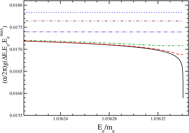
Figure 1: The “outer” radiative correction $g(\Delta E,E_{e},E_{e}^{\rm max})$ as a function of the electron detector resolution $\Delta E$ and the electron energy $E_{e}$ in the endpoint region of tritium $\beta$-decay. The solid line is Sirlin’s result [19], for which $\Delta E=0$. The dotted line corresponds to Vogel’s result [21], for which $\Delta E=E_{e}^{\rm max}-m_{e}$. The remaining curves correspond to $\Delta E=1$ [6], $6$ [12], $100$, and $1000$ eV, respectively, moving in sequence from the solid line to the dotted one. The chosen values of $\Delta E$ correspond to those of the planned and recent experiments to which we refer.

We can now proceed to evaluate the changes these theoretical corrections make to the shape assumed in previous experimental assays of the $\nu$ mass. For definiteness, we also include the leading-order recoil corrections to the electron energy spectrum. We may once again adapt the results from neutron decay to this case. We adopt the notation of Bender et al. in Ref. [28], though the couplings of the hadronic weak current are now nuclear form factors evaluated at zero momentum transfer. Noting Ref. [28], we replace the absolute, squared nuclear transition matrix element, which we have taken to be $|{\cal M}|^{2}=|{\cal M}_{0}|^{2}=g_{V}^{2}+3g_{A}^{2}$, with

$$|{\cal M}|^{2}\to|{\cal M}_{0}|^{2}(1+{\cal R})\;,$$ (14)

where

$$\!\!\!\!\!\!\!\!{\cal R}=\frac{1}{(g_{V}^{2}+3g_{A}^{2})}\Bigg{[}g_{A}f_{2}\left(-4\frac{m_{e}^{2}}{M_{A}E_{e}}-4\frac{E_{e}^{\rm max}}{M_{A}}+8\frac{E_{e}}{M_{A}}\right)+g_{V}^{2}\left(2\frac{E_{e}}{M_{A}}\right)$$

$$\!\!\!\!\!\!\!\!+g_{A}^{2}\left(-2\frac{m_{e}^{2}}{M_{A}E_{e}}-2\frac{E_{e}^{\rm max}}{M_{A}}+10\frac{E_{e}}{M_{A}}\right)+g_{V}g_{A}\left(-2\frac{m_{e}^{2}}{M_{A}E_{e}}-2\frac{E_{e}^{\rm max}}{M_{A}}+4\frac{E_{e}}{M_{A}}\right)\Bigg{]}\,.$$ (15)

Note that $M_{A}=2809.4319$ MeV [29] is the tritium mass and $E_{e}^{\rm max}-m_{e}=18.57$ keV [15], so that $E_{e}^{\rm max}/M_{A}\sim 1.9\cdot 10^{-4}$. Since $|{\cal M}_{0}|^{2}$ can be absorbed into the overall normalization of the decay rate, the function ${\cal R}$ represents the first appearance of nuclear-structure effects in the prediction of the electron-energy spectrum in tritium $\beta$-decay. The form factors which enter are largely determined by the symmetries of the Standard Model (SM), so that the subsequent uncertainty in the predicted recoil correction, which is itself of small numerical size, is very small. In writing Eq. (15), we have assumed the validity of the conserved-vector-current (CVC) hypothesis and have neglected the form factors associated with second-class-current contributions. In the context of the SM, this is tantamount to neglecting the effects of isospin violation, so that the recoil term is subject to corrections of ${\cal O}(1\%)$. The vector coupling $g_{V}$ is also unity by the CVC hypothesis; the computed correction due to charge-symmetry breaking in the overlap of the ³H-³He wave functions, due to Towner, is $\delta_{c}=0.06\%$ [31]; we note $g_{V}^{2}={g_{V}^{\prime}}^{2}(1-\delta_{c})$, where ${g_{V}^{\prime}}^{2}$ absorbs the inner radiative correction $\Delta_{R}$ and $|V_{ud}|^{2}$, with $V_{ud}$ a CKM matrix element. The CVC hypothesis determines the weak-magnetism coupling $f_{2}$ from the measured ³H and ³He magnetic moments [29], to yield $f_{2}/g_{V}^{\prime}=-3.0533$; we ignore the possibility of a inner radiative correction idiosyncratic to $f_{2}$. The ³H half-life determines $g_{V}^{2}+3g_{A}^{2}$ up to corrections of recoil order; this is sufficient to determine the couplings which appear in the recoil-order expression. In specific, we have [31] $(1-\delta_{c}+3g_{A}^{2}/{g_{V}^{\prime}}^{2})^{-1}=G_{F}^{2}{g_{V}^{\prime}}^{2}f(1+\delta_{R})t_{1/2}/K$ with ${g_{V}^{\prime}}^{2}=(1+\Delta_{R})|V_{ud}|^{2}$ and $K=2\pi^{3}\ln 2/m_{e}^{5}$. We use $G_{F}$, $\alpha$, $m_{e}$, and $\hbar$ as given in Ref. [32], $\Delta_{R}=0.0240$, $V_{ud}=0.9740$ as in Ref. [33], and the half-life $t_{1/2}=12.3$ yrs as recommended in Ref. [29]. Finally we use the integral of $F+(\alpha/2\pi)g_{S}$, noting Eq. (4) of Ref. [17] for $F$, over the allowed phase space to fix $f(1+\delta_{R})$, for which we find $2.9109\cdot 10^{-6}$. We use $R_{e}=1.68$ fm throughout [30, 29]. This yields $g_{A}/g_{V}^{\prime}=1.22$; note that this ratio of couplings implicitly contains the quenching of the Gamow-Teller matrix element due to nuclear structure effects.

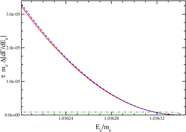
Figure 2: The change in the electron energy spectrum, $d\Gamma/dE_{e}$, upon the inclusion of $g(\Delta E,E_{e},E_{e}^{\rm max})$, as a function of $E_{e}$. The solid line has $\Delta E=4.4$ eV as per Ref. [15]; the dashed line also includes recoil corrections as per Eq. (14). For reference the change in the theoretical form of the energy spectrum assumed in Ref. [15], if $m_{\nu}^{2}=0\to-4$ eV², is shown as the dot-dashed line as well.

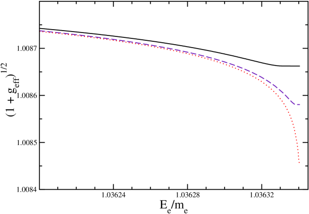
Figure 3: The ratio of the corrected to uncorrected Kurie plots, namely $(1+g_{\rm eff})^{1/2}$, with $g_{\rm eff}\equiv{\cal R}+(\alpha/2\pi)g(\Delta E,E_{e},E_{e}^{\rm max})$, as a function of $E_{e}$. The solid line has $\Delta E=4.4$ eV, the dashed line has $\Delta E=1$ eV, and the dotted line has $\Delta E=0.1$ eV.

Armed with these results, we now proceed to evaluate the change in the electron energy spectrum upon the inclusion of the outer radiative correction, $g(\Delta E,E_{e},E_{e}^{\rm max})$. We illustrate $\Delta(d\Gamma/dE_{e})=(d\Gamma_{0}/dE_{e})\alpha g(\Delta E,E_{e},E_{e}^{\rm max})/(2\pi)$ in Fig. 2, using the energy resolution of the Mainz experiment [15], $\Delta E=4.4$ eV. In this figure, the inclusion of the $\Delta E$ dependence is of little impact; the resulting curve is hardly distinguishable from that which results from the use of Sirlin’s function, Eq. (3). The recoil corrections are included as well, so that we employ $d\Gamma/dE_{e}=d\Gamma_{0}/dE_{e}(1+{\cal R}+F+\alpha/(2\pi)g(\Delta E,E_{e},E_{e}^{\rm max}))$; they are rather small, though they are appreciable. The analysis of Ref. [15] assumes the theoretical form given in Eq. (1), inferring $m_{\nu}^{2}=-3.7\pm 5.3\pm 2.1$ eV² from their experimental data. Thus, for reference, we also show $\Delta(d\Gamma/dE_{e})=d\Gamma_{F}(m_{\nu}^{2}=-4\hbox{eV}^{2})/dE_{e}-d\Gamma_{F}(m_{\nu}^{2}=0\hbox{eV}^{2})/dE_{e}$ in Fig. 2. Note that employing $m_{\nu}^{2}>0$ yields a $\Delta(d\Gamma/dE_{e})$ which differs in sign from that generated with $g(\Delta E,E_{e},E_{e}^{\rm max})$. It is apparent that the change in the theoretical energy spectrum due to the neglected ${\cal O}(\alpha)$ correction acts to increase the electron energy spectrum; this effect is also realized through a negative value of $m_{\nu}^{2}$ in Eq. (1). The neglect of the outer radiative correction generates a negative shift in $m_{\nu}^{2}$. We emphasize that this shift is a consequence of the change in shape in the electron energy spectrum induced by the outer radiative correction. We illustrate this in Fig. 3, in which we show the ratio of the corrected to uncorrected Kurie plots, recalling that the Kurie plot is $K(E_{e})\equiv[(d\Gamma/dE_{e})(1/Fp_{e}E_{e})]^{1/2}$ versus $E_{e}$. This ratio is simply $(1+g_{\rm eff})^{1/2}$ to ${\cal O}(\alpha)$, where $g_{\rm eff}\equiv{\cal R}+(\alpha/2\pi)g(\Delta E,E_{e},E_{e}^{\rm max})$.

To estimate the impact of the remaining ${\cal O}(\alpha)$ correction on the value of the neutrino mass, we introduce the fit function used in earlier work [15]:

$$\tau m_{e}\frac{d\Gamma}{dE_{e}}=Am_{e}^{-4}F(Z,R_{\rm e},E_{e})p_{e}E_{e}(E_{e}^{\rm max}-E_{e})\sqrt{(E_{e}^{\rm max}-E_{e})^{2}-m_{\nu}^{2}}+B\,,$$ (16)

where $A$, $E_{e}^{\rm max}$, $m_{\nu}^{2}$, and $B$ are all fit to the electron energy spectrum. For our comparison, which we effect for purposes of illustration, we have neglected the contributions associated with the excited final states of the daughter ³He⁺ - T molecule and include the elastic contribution only. Note that $B$ represents a constant experimental background, so that we set $B=0$. Fitting the remaining parameters in Eq. (16) to the dashed curve in Fig. 2 yields the comparisons shown in Fig. 4. We fit the last 70 eV of the electron energy spectrum and set $\Delta E$=4.4 eV, in an attempt to simulate the conditions in Sec. 6.3 of Ref. [15], for which $m_{\nu}^{2}=-3.7\pm 5.3\pm 2.1$ eV² was inferred. We fit the quantity $\tau m_{e}d\Gamma/dE_{e}$, where the lifetime $\tau$ is $\tau=t_{1/2}/\ln{2}$, noting, for reference, that $A=3.43537\cdot 10^{5}$ in our theoretical curves. Using the MIGRAD minimization program in the CERN package ROOT [34], we find two different fits of comparable quality, which possess very different values of $m_{\nu}^{2}$; apparently a significant shift in $m_{\nu}^{2}$ can be accommodated by normalizations $A$ which differ by $\sim 2$%. In both cases $m_{\nu}^{2}<0$; we cannot successfully fit our curves using a non-negative value of $m_{\nu}^{2}$ in Eq. (16). In constrast, if we fit Eq. (16) to a curve containing the Fermi function only, these features do not occur. In this case, we find fits with $|m_{\nu}^{2}|<1$ eV² are consistent with the input curve; $m_{\nu}^{2}$ need not be negative definite.

The refinements we have introduced, namely, the $\Delta E$ dependence to the outer radiative corrections cum the recoil corrections, shift $m_{\nu}^{2}$ at no larger than the ${\cal O}(1\,\hbox{eV}^{2})$ level. As Fig. 3 makes clear, this conclusion is sensitive to the precise value of $\Delta E$, as well as the interval in $E_{e}$ over which the neutrino mass is fit. For other choices of these parameters, their relative impact could be more significant. Given the results shown in Fig. (4), we cannot make a robust conclusion concerning the absolute scale of the shift in $m_{\nu}^{2}$ our previously neglected theoretical corrections would induce in a more realistic analysis; nevertheless, we can say that the consequence of neglecting these terms is to push $m_{\nu}^{2}<0$ in an artificial way. We presume that with the replacement of Eq. (16) with a fit function incorporating the radiative and recoil corrections we have calculated such artificial shifts would disappear. In the analysis we have effected, this turns out to be the case.

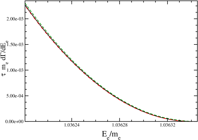
Figure 4: The electron energy spectrum for $E_{e}^{\rm max}-E_{e}\leq 70$ eV, as a function of $E_{e}$. The solid curve shows the theoretical spectrum to be fit, which includes $g(\Delta E,E_{e},E_{E}^{\rm max})$ with $\Delta E$=4.4 eV and recoil corrections as per Eqs. (14,15). The dashed curve is realized from Eq. (16) using $E_{e}^{\rm max}=18.57$ keV, $A=3.55020\cdot 10^{5}$, and $m_{\nu}^{2}=-67$ eV². In constrast, the dot-dashed curve has $A=3.49446\cdot 10^{5}$ and $m_{\nu}^{2}=-0.01$ eV².

In this letter we have evaluated the ${\cal O}(\alpha)$ outer radiative correction, $g(\Delta E,E_{e},E_{e}^{\rm max})$, to the electron energy spectrum in ³H $\beta$-decay, so that $(\alpha/2\pi)g+F-1$, where $F$ is the Fermi function, constitutes the complete ${\cal O}(\alpha)$ correction to the electron energy spectrum. We have updated the calculation of Sirlin [19] to include the dependence of the outer radiative correction on the detector energy resolution $\Delta E$; as a consequence the ${\cal O}(\alpha)$ correction we compute to the shape of the electron energy spectrum is finite as $E_{e}\to E_{e}^{\rm max}$. However, as necessary, it has no impact on the radiative correction to the total decay rate. Interestingly, the outer radiative correction was omitted all together in earlier studies of tritium $\beta$-decay [8, 9, 10, 11, 12, 13, 14, 15, 6]; we have shown that the shape correction associated with this $\sim 2\%$ shift mimicks a negative value of $m_{\nu}^{2}$. We believe it is necessary to update earlier experimental analyses to take this theoretical correction into account, to realize an accurate determination of the neutrino mass. A highly accurate theoretical spectrum can be found by modifying Eq. (1), the form used in earlier experimental analyses of ³H $\beta$-decay, through the substitution $F\to F^{\ast}+(\alpha/2\pi)g(\Delta E,E_{e},E_{e}^{\rm max})+{\cal R}$, using Eqs. (8-13) and Eq. (15). Our focus has been on $g(\Delta E,E_{e},E_{e}^{\rm max})$ and ${\cal R}$; theoretical corrections to these terms accrue from i) ${\cal O}(Z\alpha^{2})$ corrections, which are known [27], and ii) ${\cal O}(1\%)$ corrections to the recoil-order term, Eq. (15), but such corrections would appear beyond the scope of current and planned experiments. The corrected Fermi function $F^{\ast}$, which includes corrections such as those due to the finite nuclear size and to charge screening of the nuclear charge by atomic electrons, is detailed in Ref. [35]; recoil corrections [28] and outer radiative corrections, as calculated by Sirlin [19], are considered in this reference as well. The outer radiative corrections are the largest of these corrections [35]. Realistic experimental conditions demand that Eq. (16), as well as the fit form we advocate, be adapted to include the population of all the excited final states $i$ of the daughter He⁺-T molecule; the excitation energies and amplitudes are computed from atomic theory. As a consequence, the elucidation of the neutrino mass in ³H $\beta$-decay relies on atomic physics input which cannot be wholly subjected to exhaustive, independent empirical test. Nevertheless, from the viewpoint of the theoretical radiative and recoil corrections, a sub-eV determination of the neutrino mass should be possible.

Acknowledgements

The work of S.G. is supported in part by the U.S. Department of Energy under contract number DE-FG02-96ER40989. We thank Wolfgang Korsch for helpful discussions and much-needed assistance with ROOT and Christian Weinheimer for useful comments and correspondence. S.G. thanks the SLAC theory group for hospitality during the completion of this manuscript. We are grateful to Burton Richter for suggestions helpful in improving our presentation.

References

[1]
[2]
Y. Fukuda et al. [Super-Kamiokande Collaboration],
Phys. Rev. Lett. 81 (1998) 1562.
[3]
Q. R. Ahmad et al. [SNO Collaboration],
Phys. Rev. Lett. 89 (2002) 011301.
[4]
K. Eguchi et al. [KamLAND Collaboration],
Phys. Rev. Lett. 90 (2003) 021802.
[5]
A. Pierce and H. Murayama,
Phys. Lett. B 581 (2004) 218;
S. Hannestad,
JCAP 0305 (2003) 004.
[6] A. Osipowicz et al. [KATRIN Collaboration],
arXiv:hep-ex/0109033.
[7]
R. G. H. Robertson and D. A. Knapp,
Ann. Rev. Nucl. Part. Sci. 38 (1988) 185.
[8]
R. G. H. Robertson et al.,
Phys. Rev. Lett. 67 (1991) 957.
[9]
H. Kawakami et al., Phys. Lett. B 256 105 (1991).
[10]
E. Holzschuh et al., Phys. Lett. B 287 381 (1992).
[11]
H. C. Sun et al., CJNP 15 261 (1993).
[12] Ch. Weinheimer et al.,
Phys. Lett. B 300 (1993) 210.
[13]
W. Stoeffl and D. J. Decman,
Phys. Rev. Lett. 75, 3237 (1995).
[14]
V. M. Lobashev et al.,
Phys. Lett. B 460 (1999) 219.
[15]
Ch. Weinheimer et al.,
Phys. Lett. B 460 (1999) 227.
[16]
S. M. Berman,
Phys. Rev. 112 (1958) 267;
T. Kinoshita and A. Sirlin, Phys. Rev. 113 (1959) 1652.
[17] S. Raman, C. A. Houser, T. A. Walkiewicz, and I. S.
Towner, At. Data Nucl. Data Tables 21 (1978) 567.
[18] E. J. Konopinski, The Theory of Beta Radioactivity
(Clarendon Press, Oxford, 1966); H. Schopper, Weak Interactions
and Nuclear Beta Decay (North-Holland, Amsterdam, 1969).
[19] A. Sirlin, Phys. Rev. 164 (1967) 1767.
[20] W. W. Repko and C. Wu, Phys. Rev. C 28 (1983) 2433;
note also D. R. Yennie, S. C. Frautschi, and H. Suura,
Ann. Phys. 13 (1961) 379.
[21]
P. Vogel,
Phys. Rev. D 29 (1984) 1918.
[22]
I. S. Towner,
Phys. Rev. C 58 (1998) 1288.
[23] J. F. Beacom and S. J. Parke,
Phys. Rev. D 64 (2001) 091302.
[24]
A. Kurylov, M. J. Ramsey-Musolf, and P. Vogel,
Phys. Rev. C 65 (2002) 055501.
[25]
M. Passera,
Phys. Rev. D 64 (2001) 113002.
[26]
V. Bernard, S. Gardner, U.-G. Meißner, and C. Zhang,
Phys. Lett. B 593 (2004) 105.
[27]
W. Jaus and G. Rasche, Nucl. Phys. A 143 (1970) 202;
W. Jaus, Phys. Lett. 40 (1972) 616;
A. Sirlin and R. Zucchini, Phys. Rev. Lett. bf 57 (1986) 1994;
W. Jaus and G. Rasche,
Phys. Rev. D 35 (1987) 3420;
A. Czarnecki, W. J. Marciano, and A. Sirlin,
arXiv:hep-ph/0406324.
Recall that the additive
radiative correction is defined
as what remains after the product is computed.
[28]
S. M. Bilen’kii et al., Sov. Phys. JETP 37 (1960) 1241;
I. Bender, V. Linke, and H. J. Rothe, Z. Phys. 212 (1968) 190.
[29]
http://www.tunl.duke.edu/NuclData/
[30] H. Collard et al., Phys. Rev. Lett. 11
(1963) 132.
[31] J. J. Simpson, Phys. Rev. C 35 (1987) 752.
[32]
K. Hagiwara et al. [Particle Data Group Collaboration],
Phys. Rev. D 66 (2002) 010001.
[33]
I. S. Towner and J. C. Hardy,
arXiv:nucl-th/9809087.
[34] http://root.cern.ch/
[35] D. H. Wilkinson, Nucl. Phys. A 526 (1991) 131.