SLAC-PUB-10510 July 2004

Monte Carlo Exploration of Warped Higgsless Models

J.L. Hewett^a, B. Lillie^b, and T.G. Rizzo^c

Stanford Linear Accelerator Center, 2575 Sand Hill Rd., Menlo Park, CA, 94025

We have performed a detailed Monte Carlo exploration of the parameter space for a warped Higgsless model of electroweak symmetry breaking in 5 dimensions. This model is based on the $SU(2)_{L}\times SU(2)_{R}\times U(1)_{B-L}$ gauge group in an AdS₅ bulk with arbitrary gauge kinetic terms on both the Planck and TeV branes. Constraints arising from precision electroweak measurements and collider data are found to be relatively easy to satisfy. We show, however, that the additional requirement of perturbative unitarity up to the cut-off, $\simeq 10$ TeV, in $W_{L}^{+}W_{L}^{-}$ elastic scattering in the absence of dangerous tachyons eliminates all models. If successful models of this class exist, they must be highly fine-tuned.

1 Introduction

As the time of the LHC turn-on draws nearer, the search for alternative theories to the standard single Higgs boson picture of electroweak symmetry breaking is intensifying. One such scenario [1] is particularly appealing in that it employs a minimal particle content in a 5-dimensional spacetime and exploits the geometry of the additional dimension to break the electroweak symmetry. The model is based on the Randall-Sundrum framework [2] with an $SU(2)_{L}\times SU(2)_{R}\times U(1)_{B-L}$ gauge group in 5-d Anti-de Sitter space. The AdS₅ slice is bounded by two branes, with the scale of physics on the IR(TeV)-brane being given by $\Lambda_{\pi}\equiv\overline{M}_{Pl}e^{k\pi r_{c}}$, with $k$ corresponding to the RS curvature parameter and $r_{c}$ being the radius of the compactified dimension. The set of boundary conditions, which differ for the two branes, generate the breaking chain $SU(2)_{R}\times U(1)_{B-L}\rightarrow U(1)_{Y}$ at the Planck scale with the subsequent breaking $SU(2)_{L}\times U(1)_{Y}\rightarrow U(1)_{QED}$ at the TeV scale. The electroweak symmetry is thus broken without the introduction of a Higgs field. After the Planck scale symmetry breaking occurs, a global $SU(2)_{L}\times SU(2)_{R}$ symmetry is present in the brane description. This breaks on the TeV-brane to a diagonal group $SU(2)_{D}$ which corresponds [3] to the custodial $SU(2)$ symmetry of the Standard Model (SM) and helps preserve the SM tree-level relation $\rho=1$. We denote this scenario as the Warped Higgsless Model (WHM).

In this scenario, the role of the Goldstone boson in generating masses for the $W$ and $Z$ bosons is played by the would be zero-mode of the KK tower corresponding to the $5^{th}$ component of the bulk gauge fields (i.e., $A^{5}_{0}$). The $Z$ boson observed at LEP/SLC/Tevatron is the first excitation of a neutral gauge boson KK tower, while the photon corresponds to the massless zero-mode of this tower. The $W$ boson observed in experiments is then the first state of a KK tower of charged gauge bosons, and there is no charged massless zero-mode. The experimentally observed values of the $W$ and $Z$ masses and couplings are essentially reproduced in this model. However, the presence of the gauge KK states affect a number of processes. In particular, much work has been performed analyzing the contributions to the set of precision electroweak measurements in Higgsless scenarios [4, 5, 6, 7, 8, 9, 10, 11, 12]. In the flat space analog of the WHM [13], i.e., a Higgsless model based on a flat higher dimensional spacetime, unacceptably large deviations from precision electroweak data are generated. However, good agreement with the data can be obtained at tree-level in the warped Higgsless scenarios, provided that the masses of the KK excitations are sufficiently heavy. In addition, the KK excitations must satisfy the constraints from direct production of new gauge bosons at the Tevatron and from their contribution to contact interactions in four fermion processes at LEPII.

Note that precision observables are sensitive to one-loop electroweak effects. In general, the loop corrections in this model will be qualitatively similar to those in the SM (up to small shifts in the couplings). However, there are three types of loop corrections that may cause large deviations: the gauge KK excitations, the absence of loops with a physical higgs, and the top quark. Since the gauge KKs are playing the role of the physical Higgs in WW scattering, it is expected that they will do the same here, so the first two effects should largely cancel. In our model all fermions are localized to the Planck brane, and the parameters of the model are adjusted so the couplings are as close to the SM couplings as possible. Hence, the top corrections should again approximate the Standard Model values. (In a model where the top mass is generated on the TeV brane [14] a more careful treatment would be needed.) Since we expect all loop corrections to qualitatively approximate the SM corrections, we will require that the tree level WHM approximate the tree level SM as closely as possible in the analysis below.

In the absence of a Higgs boson, or any other new physics, perturbative unitarity (PU) in elastic $W_{L}^{+}W_{L}^{-}$ scattering is violated at an energy scale of $\simeq 1.7$ TeV. However, in these Higgsless scenarios, it is in principle possible that the exchange of the neutral gauge KK tower in $W_{L}^{+}W_{L}^{-}\rightarrow W_{L}^{+}W_{L}^{-}$ can restore PU, provided that a set of conditions on the KK masses and couplings are satisfied [13]. This works well in the flat space analog of the WHM, but is problematic within the warped scenario. In particular, the region of parameter space which enjoys good agreement with the precision electroweak and collider data leads to low-scale ($\sim 2$ TeV) perturbative unitarity violation (PUV) in gauge boson scattering [6]. One would at least expect the theory to remain perturbative up to the cutoff scale of the effective theory on the TeV-brane, $\Lambda_{\pi}$, where $\Lambda_{\pi}$ is roughly on the order of 10 TeV. This leads to a tension in the model parameter space in terms of finding a region which simultaneously satisfies all of the model building requirements as well as the experimental constraints.

In [8, 15] the effects of including the IR-brane terms associated with the $U(1)_{B-L}$ and $SU(2)_{D}$ gauge symmetries were examined; the presence of such terms is known to alter the corresponding KK spectrum and couplings [16]. In these analyses it was found that the addition of the $U(1)_{B-L}$ IR-brane term could lead to improved agreement with the electroweak data [8] and the inclusion of the $SU(2)_{D}$ brane term could delay PUV in $W_{L}^{+}W_{L}^{-}\rightarrow W_{L}^{+}W_{L}^{-}$ to scattering energies of order $\sim 6-7$ TeV [15]. However, a scan of the full parameter space was not performed in order to determine whether there exists a region where all the constraints discussed above are simultaneously satisfied.

In this paper, we perform a detailed exploration of the WHM parameter space via Monte Carlo techniques. There are a number of parameters present in this scenario: (i) the set of coupling strengths for each gauge symmetry: $g_{5L}$ which is fixed by $G_{F}$, the ratio $\lambda\equiv g_{5B}/g_{5L}$ which is fixed by the value of $M_{Z}$, and the ratio $\kappa\equiv g_{5R}/g_{5L}$ which lies in the restricted range $0.75\,\,\hbox to0.0pt{\raise 3.0pt\hbox{$<$}\hss}{\lower 3.0pt\hbox{$\sim$}}\,\,\kappa\,\,\hbox to0.0pt{\raise 3.0pt\hbox{$<$}\hss}{\lower 3.0pt\hbox{$\sim$}}\,\,4.0$, but is otherwise free. (ii) The brane kinetic terms associated with the IR-brane, $\delta_{B,D}$, and the UV-brane, $\delta_{L,Y}$. Here the brane terms will be treated as free phenomenological parameters but should in principle be calculable from the full theory once the UV-completion is known. The parameter space is sufficiently large such that it is best scanned by Monte Carlo sampling. For each set of parameters, we subject the model to a succession of tests: (i) model requirements, such as the absence of ghosts and tachyon states, (ii) consistency with the precision electroweak data, (iii) consistency with the direct and indirect collider bounds on new gauge boson production, and (iv) PU in elastic $W_{L}^{+}W_{L}^{-}$ scattering. In particular, we require that this scattering process be unitary up to $\Lambda_{\pi}\simeq 10$ TeV. We find that the conditions (i-iii) are relatively easy to simultaneously satisfy, but that none of the models satisfied perturbative unitarity beyond the scale of $\simeq 2$ TeV. We conclude that if a successful model of this type exists, it must be highly fine-tuned, or must contain other sources of new physics.

We present our analysis in the next two sections. The formalism of the WHM is presented in detail in our earlier work [6, 15] and will not be reproduced here.

2 Analysis: Electroweak and Collider Constraints

As discussed above, the model in its present form contains five free parameters: $\kappa=g_{R}/g_{L}$, the ratio of the two $SU(2)_{L,R}$ gauge couplings which is expected to be of order unity, and the four brane kinetic term parameters, $\delta_{B,D,L,Y}$, corresponding to the various unbroken gauge groups on the TeV and Planck branes: $U(1)_{B-L},SU(2)_{D},SU(2)_{L}$ and $U(1)_{Y}$, respectively. Our approach is to choose a value for $\kappa$ and then explore the parameter space spanned by $\delta_{B,D,L,Y}$ via Monte Carlo methods. To be definitive we will assume that all the $\delta_{i}$ are constrained to lie in the range $-\pi kr_{c}\leq\delta_{i}\leq\pi kr_{c}$ as suggested in [16], and we fix $kr_{c}=11.27$ in our numerical study. For each set of values of the $\delta_{i}$ we define a successful model as one which passes through a number of cuts and filters that we now describe in some detail. Our results are compiled in Tables 1 and 2, which displays the amount of statistics generated for each value of $\kappa$ and the number of models which survive each successive constraint. Our statistics are concentrated near $\kappa=1$ as in this case the KK spectrum is relatively light and we are more hopeful that PU constraints will be satisfied.

Upon generating a set of $\delta_{i}$ we first calculate a group of model parameters which are associated with the lightest massive charged and neutral gauge bosons, and ensure that they are identified with the observed SM fields, $W_{1}=W$ and $Z_{1}=Z$. We take the experimental values of their masses $M_{Z}=91.1875$ GeV and $M_{W}=80.426$ GeV [17] as input to our analysis. This numerically fixes the low energy scale $ke^{-\pi kr_{c}}$ that gives the masses of the KK excitations in the RS model, as well as the value of the on-shell weak mixing angle, $\sin^{2}\theta_{OS}=1-M_{W}^{2}/M_{Z}^{2}$. Next, the requirement of the absence of ghosts in the unitary gauge of any physical theory implies that these two states, $W_{1}$ and $Z_{1}$, must have positive norms. Similarly, the field that represents the photon must also have a positive norm. In addition to these constraints, we demand that the ratio of the squares of the gauge couplings, $\lambda^{2}=g_{B-L}^{2}/g_{L}^{2}$, be positive definite. As can be seen from Table 1, these few simple cuts can remove as much as $\sim 40\%$ of the parameter space volume.

Assuming that the SM fermions (at least the first two generations) are localized near the Planck brane we can now calculate a number of electroweak quantities. Recall that our philosophy is that we want the tree level Higgsless model to match the tree level SM as closely as possible, outside of the Higgs sector, since in many cases we expect approximately similar one-loop radiative corrections. As we found in our earlier works [6, 15], a description of the $\gamma,W$ and $Z$ couplings to the SM matter fields can be parameterized in terms of two other definitions of the weak mixing angle in addition to $\sin^{2}\theta_{OS}$. These two additional angles are defined via: $\sin^{2}\theta_{eg}=e^{2}/g_{W}^{2}$, with $g_{W}=g_{ffW_{1}}$ being the coupling of the $W$ to SM fermions on the Planck brane, and $\sin^{2}\theta_{eff}$ being given by the couplings of the $Z$ to the same fermions at the $Z$-pole as discussed below. The electromagnetic coupling is, as usual, defined through the interaction of the massless neutral mode, $Z_{0}$, which we identify as the photon, to the SM fields. All three definitions of the weak mixing angle are identical at the tree level in the SM but are, in general, quite different numerically in the WHM.

Cuts             $\kappa$	0.75	0.9	1.0	1.25	1.5	2.0	3.0	4.0
Initial Sample	308,710	141,950	1,307,463	251,970	271,570	145,570	181,274	136,920
$\lambda^{2}>0$	130,286	62,202	585,011	115,455	125,035	67,662	82,583	16,204
No $\gamma,Z$ ghosts	130,286	62,202	585,011	115,455	125,035	67,662	82,583	16,204
$|\delta\rho|<0.005$	16,181	7,887	76,994	16,728	20,183	13,799	24,223	2,958
$|s^{2}_{\rm eff}-s^{2}_{\rm os}|<0.005s^{2}_{\rm os}$	676	387	3,665	875	1,356	1,328	3,838	2,899
$|s^{2}_{\rm eg}-s^{2}_{\rm os}|<0.005s^{2}_{\rm os}$	242	159	1,539	332	545	576	1,805	2,013
No $Z^{\prime}$ ghost	242	159	1,539	322	545	576	1,805	2,013
$Z^{\prime}$ Tevatron	150	102	1134	217	393	439	1,556	1,830
$m_{Z^{\prime}}<1.5$ TeV	74	50	644	90	180	202	828	1,581
LEPII indirect	70	45	550	72	80	175	796	1,178
Isospin coupling	24	13	112	12	8	12	65	0
No Tachyons	0	0	0	0	0	0	7	0
PUV	0	0	0	0	0	0	0	0

Table 1: Data samples and their responses to the various constraints as described in the text. The values represent the number of cases surviving each of the cuts.

Writing the $Z$-pole couplings to SM fermions as

$${g_{Z}\over{c_{OS}}}(T_{3}-\sin^{2}\theta_{eff}~{}Q)\,,$$ (1)

in obvious notation, we also can define an auxiliary quantity, $\rho_{eff}^{Z}=g_{Z}^{2}/g_{W}^{2}$, which relates the strengths of the $W$ and $Z$ gauge boson interactions. We identify $g_{Z}/c_{OS}=g_{ffZ_{1}}$. In the SM at tree-level $\rho_{eff}^{Z}=1$, of course. We note that all of the electroweak observables at the $W,Z$ mass scale can now be described in terms of the three weak mixing angles, $M_{Z}$, and $\rho_{eff}^{Z}$ and we have no need to introduce any other parameterizations. It is clear that if we wish to reproduce the tree-level SM we must have all three values of $\sin^{2}\theta$ be almost equal as well as require that $\rho_{eff}^{Z}$ be very close to unity. In our numerical study we will demand that the three definitions of $\sin^{2}\theta$ all be equal within $0.5\%$ and additionally require $|\delta\rho_{eff}^{Z}|=|\rho_{eff}^{Z}-1|$ to be less than 0.005. The magnitude of these constraints should be comparable to the size of the one-loop generated electroweak corrections. This set of constraints is extremely powerful for the full WHM parameter space, but is especially strong for low values of $\kappa$ as can be seen from Table 1; only a few percent of the original model parameter space remains after applying these cuts. Note that models with larger values of $\kappa$ are generally favored by these electroweak constraints. This is not unexpected; we saw in our earlier work that the SM limit is approached rapidly as the value of $\kappa$ is increased. The price one pays for this is a rapid increase in the masses of the KK states leading to an obvious failure in PU as discussed below.

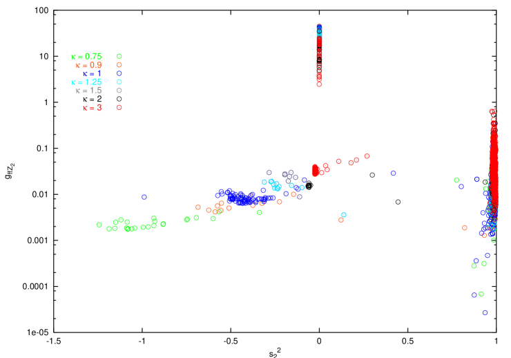
Figure 1: The coupling strength of the first neutral KK excitation beyond the $Z$ in units of $g_{W}$ as a function of its effective $\sin^{2}\theta$. The color coding labels models with different values of $\kappa$. All electroweak constraints have been applied to the cases shown as well as the bounds from the TeVII direct searches. A cut of $M_{Z_{2}}<1.5$ TeV has also been applied. Indirect LEPII constraints have not yet been imposed.

We now turn our attention to the mass and couplings of the next lightest neutral KK state, $Z_{2}$; these parameters are highly constrained by both experimental data as well as our requirement of PU as we will see below. We first impose the obvious constraints that this state not be a ghost and that it has not (yet) been observed in direct $Z^{\prime}$-like production searches at LEPII or the Tevatron[19, 20]. This places a correlated cut on the mass of this state as a function of its couplings to the SM fermions on the Planck brane. Futhermore, we note that the indirect search constraints for $Z^{\prime}$-like states must also be satisfied. To be specific we will demand that the masses of the $Z_{2}$’s as well as their couplings to SM fermions are such as to have avoided the LEPII contact interaction constraints[20]. This constraint is actually quite powerful and removes an entire region in the $Z_{2}$ mass vs. coupling plane which survives the electroweak and Tevatron bounds. After imposing all these requirements we see from Table 1 that there are a respectable number of surviving cases.

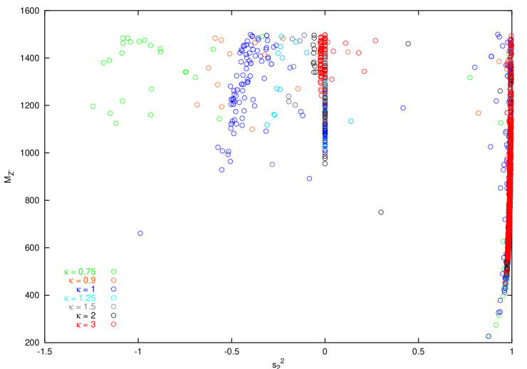
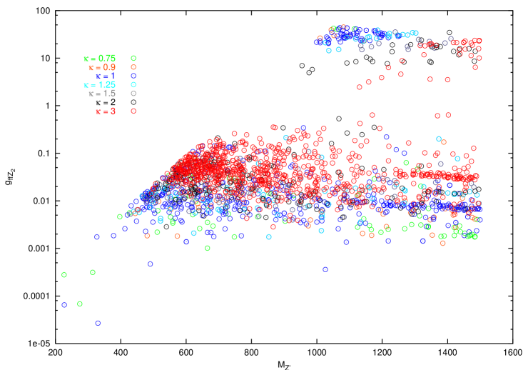
Figure 2: Same as in the previous figure but now showing the mass-coupling strength and $s_{2}^{2}$ correlations.

The particular properties of the surviving cases will be examined in detail below. Figures. 1 and 2 show the values of the $Z_{2}$ mass and coupling for those models passing all of our above cuts except the constraints imposed by LEPII; in these figures an additional requirement for PU that $M_{Z_{2}}\leq$ 1.5 TeV, to be discussed further below, has been imposed. The Tevatron direct search constraint is responsible for the sharp diagonal boundary in the bottom panel of Fig. 2. Note that the couplings of the $Z_{2}$ can always be written in a form similar to the $Z$ above except we denote the overall coupling strength as $g_{ffZ_{2}}$ and the value of the corresponding weak mixing angle as $s_{2}^{2}=\sin^{2}\theta_{eff}(Z_{2})$, i.e., $(g_{ffZ_{2}}/c_{w})(T^{f}_{3L}-s^{2}_{2}Q^{f})$. Note the large set of models near $s_{2}^{2}=0$ and 1, the former with large couplings and masses between $\sim$ 1 and 1.5 TeV. These strongly coupled cases are entirely removed by the LEPII contact interaction bound and will not concern us further. It is important to note that at this point there are a reasonable of surviving models subsequent to applying this rather strict set of electroweak and collider constraints on the model parameter space. This situation is in contrast with results previously obtained by Barbieri et al.[9] in the case of the flat space analog where no warping is present. These authors showed that there was no significant region of parameter space which simultaneously satisfied the collider and precision electroweak constraints. We have performed a Monte Carlo study of the flat space analog model, imposing the constraints presented above, and effectively confirm their results. We note for completeness that if we strengthen our electroweak cuts such that $0.5\%\rightarrow 0.1\%$ in the analysis above, the number of surviving cases is reduced by a factor $\simeq 10$.

3 Analysis: Perturbative Unitarity and Tachyons

Unitarity is an important property of any gauge theory[21, 22, 23]. Before examining PU directly, two further filters can be applied that will help us to focus on models which may satisfy our basic requirements. If the $Z_{2}$ in any of the models that survive both the electroweak and collider constraints is to contribute significantly to the $W_{L}^{+}W_{L}^{-}$ amplitude it must predominantly couple to isospin and not to $B-L$ or hypercharge $Y$. Note that when $s_{2}^{2}$ is near unity(zero), the $Z_{2}$ couples almost purely to $Y$(isospin). To ensure that the $Z_{2}$ has significant isospin-like coupling, we will demand that $s_{2}^{2}<0.7$. We make exception for the special set of cases where the $Z_{2}$ mass is less than $\simeq 400$ GeV. The reason for keeping these $B-L$-like coupled states is that their light masses may help induce a potentially large contribution to the $W_{L}^{+}W_{L}^{-}$ elastic scattering amplitude. Furthermore, there may exist somewhat heavier excitations not too far away in mass which are coupled to isospin. This cut on $s_{2}^{2}$ appears to be rather loose, but many of the surviving models have great difficulty satisfying it. It is interesting to note that at this point in the parallel analysis of the flat space analog model [13] none of the cases satisfy this constraint; all of the possible cases in the flat space model surviving both collider and electroweak constraints are found to essentially couple to $B-L$ or $Y$.

In addition to the above, the $Z_{2}$ satisfying the collider constraints must still be sufficiently light as to make a significant contribution to $W_{L}^{+}W_{L}^{-}$ elastic scattering. Recall that in the SM without a Higgs boson, PUV occurs near $\sqrt{s}\simeq 1.7$ TeV. This implies that there must be at least one, and more likely several, neutral KK states below this scale if they are to ‘substitute’ for the SM Higgs in restoring unitarity. We thus impose the rather weak requirement that the lightest new neutral KK state, $Z_{2}$, must exist with a mass below 1.5 TeV; we make no further requirements on the spectrum for now.

This pair of constraints on the mass and nature of the $Z_{2}$ couplings are rather difficult to satisfy simultaneously for the models that have passed the electroweak and collider cuts; relatively few cases survive at this point as can be seen from Table 1. Most of the models passing the electroweak and collider bounds tend to be either too massive or predominantly coupled to hypercharge. We can also see this from Figs. 1 and 2 where the densely populated region near $s_{2}^{2}=1$ with a mass greater than 400 GeV is now removed by these cuts. At this point, the remaining models are presented in Figs. 3 and 4; their distribution in $\delta_{i}$ space is shown in Fig. 5.

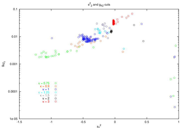
Figure 3: Same as Fig.1, but now applying the constraints from LEPII and the correlated mass-$s_{2}^{2}$ cuts to remove the KK states coupling to $B-L$ and hypercharge as described in the text.

At this point we are ready to examine the PU characteristics of the remaining cases shown in Figs. 3-5 in detail. First we note that these models fall into two broad classes: those few with all positive $\delta_{i}$ and those with at least one of the $\delta_{i}$ being negative. An analysis of PU in $W_{L}^{+}W_{L}^{-}$ elastic scattering for the cases with all positive $\delta_{i}$ follows the standard procedure described in our earlier work [6, 15] which makes use of the scattering amplitude as given by [24] augmented to include additional neutral KK exchanges. Our proceedure is to calculate the complete amplitude using the expressions of Duncan et al.[24] which we modify to include an an arbitrary number of neutral KK exchanges in the $s-$ and $t-$ channels as well as an arbitrary $W$ 4-point coupling. We then integrate this amplitude to extract out the $J=0$ patial wave, $a_{0}$, subject to angular integration cuts imposed to avoid the photon $t-$channel pole. For our test of PU we demand that $|Re~{}a_{0}|<1/2$, as is widely done in the literature. This analysis reveals that none of these models are much improved in comparison to the SM without a Higgs boson, i.e., PUV occurs at $\simeq 2$ TeV. The main reason for this is that these cases tend to have a light $Z_{2}$ which is predominantly coupled to $Y$ as discussed above. To restate, if the $\delta_{i}$ are all chosen positive, the models surviving the electroweak and collider constraints do not lead to theories which have PU beyond the $\simeq 2$ TeV scale.

Cuts             $\kappa$	1.0	1.5	2.0	2.5	2.75	3.0	4.0
Initial Sample	611,150	304,680	178,320	122,801	266,801	169,862	70,661
$\lambda^{2}>0$	611,150	304,680	178,320	122,801	266,801	169,862	70,661
No $\gamma,Z$ ghosts	611,150	304,680	178,320	122,801	266,801	169,862	70,661
$|\delta\rho|<0.005$	168,732	159,537	107,709	89,124	211,944	146,087	69,867
$|s^{2}_{\rm eff}-s^{2}_{\rm os}|<0.005s^{2}_{\rm os}$	0	502	1,506	2,734	8,600	7,456	8,724
$|s^{2}_{\rm eg}-s^{2}_{\rm os}|<0.005s^{2}_{\rm os}$	0	244	760	1,505	4,887	4,308	5,317
No $Z^{\prime}$ ghost	0	244	760	1,505	4,887	4,308	5,317
$Z^{\prime}$ Tevatron	0	6	145	530	2,204	2,233	4,174
$m_{Z^{\prime}}<1.5$ TeV	0	6	143	530	2,086	2,112	3,919
LEPII indirect	0	6	143	509	2,086	2,112	3,919
Isospin coupling	0	0	0	0	0	0	0
No Tachyons	0	0	0	0	0	0	0
PUV	0	0	0	0	0	0	0

Table 2: Same as the previous table but now for a special set of runs assuming all the $\delta_{i}\geq 0$. Note that many cases survive until the $B-L$ or $Y$ cut is employed.

In order to verify this result we generated a larger statistical sample, an additional $\sim 1.7\cdot 10^{6}$ models, distributed over various values of $\kappa$, assuming all of the $\delta_{i}\geq 0$. The results from performing these runs are shown in Table 2 using the same cuts as above. Here we see that although many models pass the combined collider and electroweak constraints none of them survive the non-$B-L/Y$ coupling requirement. Thus all of these models fail, confirming our previous results. We checked that this also occurs in the analog flat space model.

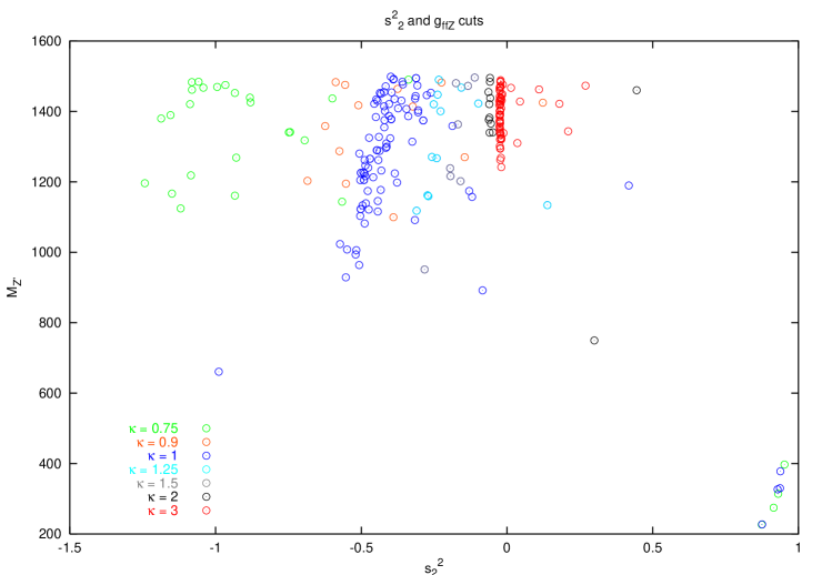
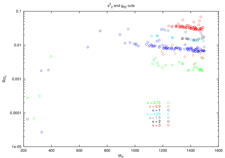
Figure 4: Same as in the previous figure but now showing the alternate projections in the mass-coupling strength-$s_{2}^{2}$ parameter space.

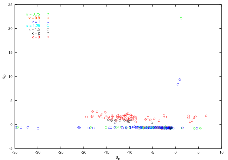
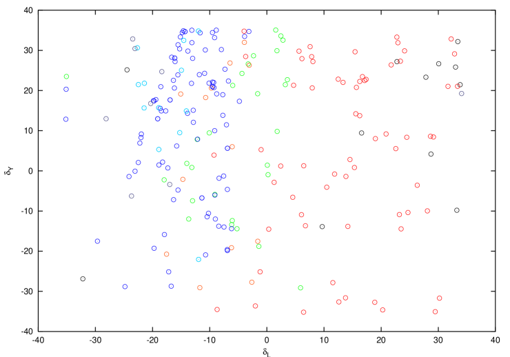
Figure 5: Same as in the previous figure but now showing the values of the $\delta_{i}$ for the surviving models..

We now return to the models with at least one negative $\delta_{i}$. Ordinarily, such models would not be considered since having negative $\delta_{i}$ at the tree-level implies the existence of tachyons with all their related difficulties [25]. Indeed, we have verified numerically that such tachyonic states do indeed exist in the spectrum for all the models in this class, and found that the tachyon masses are quite sensitive to the magnitudes of the $\delta_{i}$. Nomura [4], however, has argued that potentially large and negative boundary terms associated with the Planck brane may be benignly generated at loop level without the significant influence of tachyons. These negative brane terms can be of sufficient importance numerically as to require their inclusion in a detailed tree-level analysis such as we are performing here. In such a case one could view the existence of tachyons as an artifact of including only partial one-loop effects. Since we are ignorant of the possible origin of negative $\delta_{i}$ in the full UV-completed theory, we must in principle consider these cases further.

When analyzing the models with negative $\delta_{i}$, one has to take care that the existence of tachyons at the tree level does not have important phenomenological effects, e.g., tachyons that have significant couplings to SM fermions or which contribute substantially to SM processes such as $W_{L}^{+}W_{L}^{-}$ scattering. At the very least, if we are to consider models with such states, the tachyons must be truly benign. Certainly models where these tachyons can lead to important physical effects must not be allowed. However, if the tachyons are significantly decoupled from the SM fields we will consider such theories as benign and examine their PU properties. Based on the analysis of Nomura [4], as well as our previous work [6, 15], one might suspect that the tachyons induced by Planck brane kinetic terms, $\delta_{L,Y}$, are benign while those arising from kinetic terms on the TeV-brane, $\delta_{B,D}$, may not be.

As an initial filter, we analyze the couplings of tachyons to the SM fermions localized near the Planck brane; clearly, these couplings can depend sensitively on the magnitude of the $\delta_{i}$. First, we must determine the number of tachyon states that are in the spectrum. In the flat space analog [13] of WHM it is easy to see that there can be only a single complex conjugate pair of tachyons in each of the neutral and charged KK towers; we expect this result to be equally valid in the warped case. A numerical study verifies these expectations and so we need to concern ourselves with only two tachyonic states, $T^{0}$ and $T^{\pm}$. We find that in all the sample cases examined the relevant couplings of these states to the SM fermions are suppressed by powers of $\epsilon=e^{-\pi kr_{c}}$ and are thus exponentially small. Such a result might have been anticipated since the Bessel functions of an imaginary argument, $I_{n}$ and $K_{n}$, which are needed to describe the tachyonic wavefunctions, are asymptotic to exponentials instead of sines and cosines as is case for the usual $J_{n}$ and $Y_{n}$. This suppression of couplings is similarly observed to take place in the flat space analog of the current model, though in a more modest fashion due to the absence of warping, where sinh’s and cosh’s replace the usual sines and cosines in the expression for the tachyonic wavefunctions. Thus consideration of the fermion-fermion-tachyon coupling places no additional constraints on any of the models under consideration. One should note, however, that such constraints may be of some importance in a wider class of models.

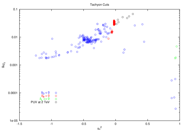
Figure 6: Same as Fig.3 but now showing the effects of removing the models with potentially dangerous tachyons. The models surviving the tachyon cuts are also shown.

As a second test we turn to $W_{L}^{+}W_{L}^{-}$ elastic scattering. Here we expect a different result as the gauge fields are in the bulk and their wave functions sample the entire region between, as well as on, the two branes. A quick way to analyze this case is to consider the contribution of the neutral tachyon to the first sum rule of Csaki et al. [13], which is one of the conditions for PU. Their derivation of this sum rule relies heavily on the completeness of the set of eigenstates of Hermitian operators; thus the neutral KK spectrum in the case of $\delta_{i}<0$ is not complete unless the tachyon state is included. Clearly as the magnitude of the negative brane terms increase the couplings of the tachyon to SM gauge fields will also increase and the tachyon will become lighter. The important issue for us is whether or not the tachyon state makes a numerically significant contribution to the sum rule.

Our results show that there are essentially three possibilities: ($i$) When $\delta_{D}<0$, we find that the tachyon makes a substantial contribution to the sum rule, which is on the order of $10\%$ or more of that of the photon, even when the magnitude of $\delta_{D}$ is small. In addition, this contribution is negative, i.e., the tachyon is also a ghost state! Certainly all such cases must be excluded. This is a powerful constraint as many of the surviving models shown in Figs. 3-5 have negative values of $\delta_{D}$ in the region near $\sim-0.7$. ($ii$) When $\delta_{L,Y}<0$, the tachyon is generally sufficiently decoupled as to make almost no significant contribution to the sum rule. Not only are the couplings weak but the masses tend to lie in the multi-TeV range. For example, when $\delta_{L}\simeq-35$, a very extreme value, the tachyon coupling to $WW$ is found to be $g_{T}^{2}\sim 10^{-6}$ which is only dangerous if the tachyon is light. For $\delta_{L}$ values of lesser magnitude the couplings are significantly smaller. This is as expected since we showed in our earlier work[6] that in, e.g., a model with $\delta_{L}\sim-7.5$, the sum rules were very well satisfied without including any tachyonic contributions. Thus we will retain all such models for further study. ($iii$) The remaining case where $\delta_{B}<0$ is a bit more problematic. As we saw in earlier [15], $\delta_{B}\neq 0$ has little influence on $W_{L}^{+}W_{L}^{-}$ elastic scattering since it only modifies the spectrum and couplings of the neutral KK’s which couple predominantly to $B-L/Y$. The tachyon $W_{L}^{+}W_{L}^{-}$ coupling is found to be generally intermediate in strength between that of the $\delta_{D}<0$ case and those for $\delta_{L,Y}<0$, unless the magnitude of $\delta_{B}$ is reasonably large $\simeq 10$. Our analysis of the surviving sample of models, however, indicates that the values of $\delta_{B}$ are indeed of this magnitude or larger. Correspondingly the masses of these states are also dangerously light implying that they can significantly contribute to SM processes. We thus drop these cases from further consideration below.

Summarizing, our numerical study confirms our expectations that the tachyons induced by negative TeV-brane kinetic terms are dangerous while those induced by the corresponding Planck brane terms are benign unless $\delta_{L}$ is very near its lower bound. Figures 6 and 7 show what little remains of our surviving models after we employ the requirement that $\delta_{B,D}\geq 0$. These 10 cases are mostly clustered (those with large negative $\delta_{Y}$) at high $Z_{2}$ masses in excess of 1.3 TeV and have pure isospin-like couplings. Those with negative $\delta_{L}$ tend to have much lighter $Z_{2}$ masses, of order less than 400 GeV. Their rather small couplings to fermions place them outside the range accessible to the Tevatron. These are the cases with small masses and large $B-L/Y$-like couplings that have survived the $B-L/Y$ cut imposed above. Unfortunately, these models all have values of $\delta_{L}\simeq-\pi kr_{c}$ and thus have light tachyons with potentially significant couplings $\sim 10^{-6}$ and are thus dropped from further consideration. This leaves only the 7 cases with negative $\delta_{Y}$ for further examination.

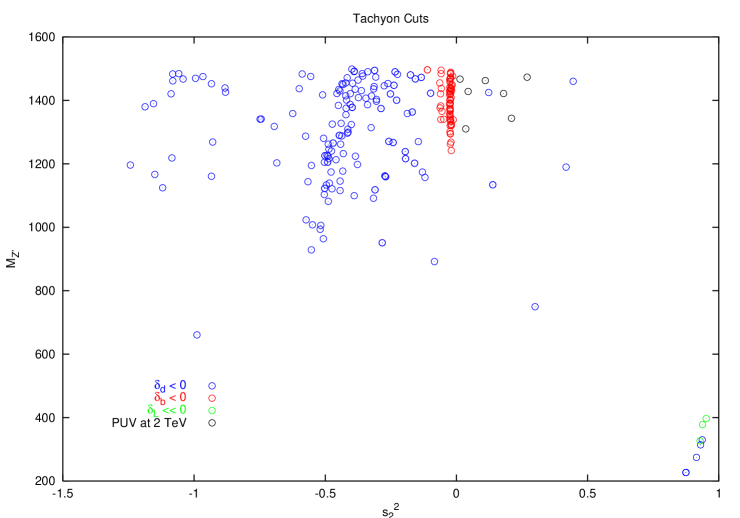
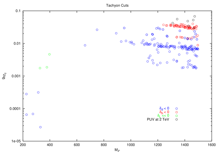
Figure 7: Same as in the previous figure but now showing the alternate projections in the mass-coupling strength-$s_{2}^{2}$ parameter space.

We now turn to the PU characteristics of these few surviving models; naively we expect all these cases to be problematic since the first KK excitation is always in excess of 1.3 TeV even though they are isospin-like coupled. Indeed all of these cases lead to PUV in the 1.9-2.2 TeV range which is not a significant improvement over the case of the SM without a Higgs boson. We thus conclude that none of the surviving models pass our PU requirements leaving us with no remaining models. Note that in obtaining these results we have not required PU to be valid up to the cutoff but only that the successful model to reasonably better than the SM without a Higgs.

Since we found that PUV occured at $\sqrt{s}\simeq 2$ TeV in the surviving models it is interesting to compare this value to that of the cutoff scale, $\Lambda$, as determined by Naive Dimensional Analysis[26], i.e.,

$$\Lambda=\epsilon{24\pi^{3}\over{g_{5L}^{2}}}\,,$$ (2)

Following the notation of our earlier work, $g_{W}^{2}=N_{\delta}g_{5L}^{2}/2\pi r_{c}$, where $N_{\delta}$ is a number near unity which depends in detail on the values of the $\delta_{i}$. With $g_{W}$ fixed via $G_{F}$ this now yields

$$\Lambda={12\pi^{2}\over{g_{W}^{2}}}{N_{\delta}\over{kr_{c}}}{k\epsilon}\,,$$ (3)

where $kr_{c}=11.27$ in our analysis. Taking typical model values we find that $\Lambda\simeq\Lambda_{\pi}\simeq 10$ TeV, which is much larger that the $\sqrt{s}$ values obtained above for PUV. Thus PUV is apparently lost long before the cutoff is reached.

4 Conclusions

In this paper we have performed a detailed tree-level Monte Carlo exploration of the parameter space of the 5-d warped Higgsless model which is based on the $SU(2)_{L}\times SU(2)_{R}\times U(1)_{B-L}$ gauge group in the Randall-Sundrum bulk. We have generated several millions of test models allowing for arbitrary gauge kinetic terms on both the Planck and TeV branes which are parameterized through the $\delta_{i}$ coefficients. As we have seen from our earlier work this scenario suffers from a serious tension between constraints arising from precision electroweak measurements and collider data as well as the requirements of perturbative unitarity in $W_{L}^{+}W_{L}^{-}$ elastic scattering up to the $\Lambda_{\pi}\sim 10$ TeV scale. We have shown that it is relatively easy to find a class of models which satisfy all of the current direct and indirect collider bounds and yet has electroweak properties which are extremely close to those of the tree-level SM. As before, the size of the parameter space that satisfies the precision EW constraints increases dramatically as $\kappa$ increases. The real difficulty arises when we require the same theories to also satisfy perturbative unitarity while being free of dangerous tachyons. Though we have generated a fairly large data sample, none of the models we have examined have been able to satisfy all of our requirements simultaneously. We do note that if a generic solution of the PUV problem is found, there appears to be enough room in the parameter space to accomodate precision EW constraints. Absent such a solution, we can thus conclude that either successful models of this type are highly fine-tuned or must include additional sources of new physics [27] which unitarizes the $W_{L}^{+}W_{L}^{-}$ scattering amplitude.

Acknowledgements

We would like to thank Csabi Csaki, Hooman Davoudiasl, Christophe Grojean, Tao Han, Graham Kribs, and John Terning for discussions related to this work. T. Rizzo would like to thank Atul Gurtu for his suggesting this type of analysis.

References

- [1] C. Csaki, C. Grojean, L. Pilo and J. Terning, “Towards a realistic model of Higgsless electroweak symmetry breaking,” arXiv:hep-ph/0308038.
- [2] L. Randall and R. Sundrum, Phys. Rev. Lett. 83, 3370 (1999) [arXiv:hep-ph/9905221].
- [3] K. Agashe, A. Delgado, M. J. May and R. Sundrum, “RS1, custodial isospin and precision tests,” JHEP 0308, 050 (2003) [arXiv:hep-ph/0308036].
- [4] Y. Nomura, “Higgsless theory of electroweak symmetry breaking from warped space,” arXiv:hep-ph/0309189.
- [5] R. Barbieri, A. Pomarol and R. Rattazzi, “Weakly coupled Higgsless theories and precision electroweak tests,” arXiv:hep-ph/0310285.
- [6] H. Davoudiasl, J. L. Hewett, B. Lillie and T. G. Rizzo, “Higgsless electroweak symmetry breaking in warped backgrounds: Constraints and signatures,” to appear in Phys. Rev D, arXiv:hep-ph/0312193.
- [7] G. Burdman and Y. Nomura, “Holographic theories of electroweak symmetry breaking without a Higgs boson,” arXiv:hep-ph/0312247.
- [8] G. Cacciapaglia, C. Csaki, C. Grojean and J. Terning, “Oblique corrections from Higgsless models in warped space,” arXiv:hep-ph/0401160.
- [9] R. Barbieri, A. Pomarol, R. Rattazzi and A. Strumia, “Electroweak symmetry breaking after LEP1 and LEP2,” arXiv:hep-ph/0405040.
- [10] R. S. Chivukula, E. H. Simmons, H. J. He, M. Kurachi and M. Tanabashi, “The structure of corrections to electroweak interactions in Higgsless models,” arXiv:hep-ph/0406077.
- [11] N. Evans and P. Membry, “Higgless W Unitarity from Decoupling Deconstruction,” arXiv:hep-ph/0406285.
- [12] R. Casalbuoni, S. De Curtis and D. Dominici, “Moose models with vanishing S parameter,” arXiv:hep-ph/0405188.
- [13] C. Csaki, C. Grojean, H. Murayama, L. Pilo and J. Terning, “Gauge theories on an interval: Unitarity without a Higgs,” arXiv:hep-ph/0305237.
- [14] C. Csaki, C. Grojean, J. Hubisz, Y. Shirman and J. Terning, “Fermions on an interval: Quark and lepton masses without a Higgs,” arXiv:hep-ph/0310355.
- [15] H. Davoudiasl, J. L. Hewett, B. Lillie and T. G. Rizzo, JHEP 0405, 015 (2004) [arXiv:hep-ph/0403300].
- [16] M. Carena, T. M. P. Tait and C. E. M. Wagner, Acta Phys. Polon. B 33, 2355 (2002) [arXiv:hep-ph/0207056]; H. Davoudiasl, J. L. Hewett and T. G. Rizzo, Phys. Rev. D 68, 045002 (2003) [arXiv:hep-ph/0212279]; JHEP 0308, 034 (2003) [arXiv:hep-ph/0305086]; M. Carena, E. Ponton, T. M. P. Tait and C. E. M. Wagner, Phys. Rev. D 67, 096006 (2003) [arXiv:hep-ph/0212307].
- [17] For a review, see M. Grünwald, “Precision electroweak measurements and fits,” talk given at APS2004, Denver, CO. May, 2004.
- [18] G. Altarelli and R. Barbieri, “Vacuum Polarization Effects Of New Physics On Electroweak Processes,” Phys. Lett. B 253, 161 (1991).
- [19] The strongest bounds at present are given by the D0 Collaboration in D0note 4375-Conf, v2.1 based on of Run II data.
- [20] The analysis of LEPII data leading to bounds on new gauge boson-like signatures can be found in C. Geweniger et al., LEP Electroweak Working Group note LEP2FF/02-03(2002)
- [21] C. Schwinn, “Higgsless fermion masses and unitarity,” arXiv:hep-ph/0402118.
- [22] J. Hirn and J. Stern, “The role of spurions in Higgs-less electroweak effective theories,” arXiv:hep-ph/0401032.
- [23] T. Ohl and C. Schwinn, “Unitarity, BRST symmetry and Ward identities in orbifold gauge theories,” arXiv:hep-ph/0312263.
- [24] M. J. Duncan, G. L. Kane and W. W. Repko, Nucl. Phys. B 272, 517 (1986).
- [25] See for example, T. Jacobson, N.C. Tsamis and R.P. Woodard, Phys. Rev. D38, 1823 (1988), and references therein.
- [26] M. Papucci, “NDA and perturbativity in Higgsless models,” arXiv:hep-ph/0408058.
- [27] S. Gabriel, S. Nandi and G. Seidl, “6D Higgsless standard model,” arXiv:hep-ph/0406020.