NLO Corrections to the $\gamma^{*}$ Impact Factor:
First Numerical Results for the Real Corrections to $\gamma_{L}^{*}$

Abstract

We analytically perform the transverse momentum integrations in the real corrections to the longitudinal $\gamma^{*}_{L}$ impact factor. The resulting integrals are Feynman parameter integrals, and we provide a MATHEMATICA file which contains the integrands. The remaining integrals are carried out numerically. We perform a numerical test, and we compute those parts of the impact factor which depend upon the energy scale $s_{0}$: they are found to be negative and, with decreasing values of $s_{0}$, their absolute value increases.

I Introduction

The NLO corrections to the ${\gamma^{*}}$ impact factor are calculated from the photon-Reggeon vertices for $q\bar{q}$ and $q\bar{q}g$ production, respectively. NLO corrections to the $q\bar{q}$ intermediate state involve the production vertex at one-loop level, $\Gamma_{\gamma^{*}\to q{\bar{q}}}^{(1)}$, These virtual corrections have been calculated in virt ; kot . As to the real corrections, the squared vertex $|\Gamma^{(0)}_{\gamma^{*}\to q{\bar{q}}g}|^{2}$ is needed at tree level; it has been computed in real and combine for longitudinal and transverse photon polarisation, respectively (cf. also fad ; kot ). In combine we have combined the infrared divergences of the virtual and of the real parts, and we have demonstrated their cancellation. What remains to complete the NLO calculation of the photon impact factor are the integrations over the $q\bar{q}$ and $q\bar{q}g$ phase space, respectively. A slightly different approach of calculating the NLO corrections of the photon impact factor has been proposed in FIK . Recently, the NLO calculation of another impact factor has been completed IKP , the impact factor for the transition of a virtual photon to a light vector meson.

In this paper we perform, for the case of the longitudinal photon polarisation, the phase space integration in the real corrections. Our aim is to have, as long as possible, analytic expressions which allow for further theoretical investigations. The main obstacle is the (infinite) integration over transverse momenta: in order to be able to perform the integration analytically, we introduce Feynman parameters. This will allow for further theoretical investigations of the photon impact factor. In particular, the Mellin transform of the real corrections w.r.t the Reggeon momentum can be calculated. This representation (together with an analogous representation of the virtual corrections) will also allow to study the impact factor in the collinear limit and to compare with known NLO results; it can also be a starting point for the resummation of the next-to-leading logs(1/x) in the quark anomalous dimensions.

Starting from the results of real , we have to integrate a sum of expressions, corresponding to products of Feynman diagrams that differ in their denominator structure. In order to introduce Feynman parameters we therefore split this sum and treat each Feynman diagram (or small groups of them) independently. This gives rise to divergences, which in the sum of all diagrams will cancel but show up in individual diagrams. The main task in the program of performing the integration analytically is the regularisation of these divergences in each individual diagram: for this we use the subtraction method. After carrying out the integration over transverse momenta we arrive at analytic expressions for each diagram. These expressions are convergent integrals over the Feynman parameters and the momentum fractions of the quark and the gluon. Since the expressions are somewhat lengthy, we do not list them in this paper but provide a MATHEMATICA code which we describe in the appendix. As a first application of our results, we carry out the remaining parameter integrals numerically and perform first tests of our calculation. In particular, we study the dependence of the photon impact factor on the energy scale which is entirely contained in the real corrections: it turns out to be in agreement with the expectations.

Our paper is organized as follows. In the next section we will recall the structure of the real corrections and specify the expressions we have to integrate, following very much the strategy described in combine . In the following section we introduce Feynman parameters and perform analytically the integration over transverse momenta. The main emphasis lies on the regularisation of the divergences, which appear in the individual diagrams. Finally, the numerical results are discussed. An appendix describes the files that provide the Feynman parameter representations of the individual diagrams.

II The real corrections

The starting point for the real corrections is the squared vertex $|\Gamma^{(0)}_{\gamma^{*}\to q{\bar{q}}g}|^{2}$ which, starting from the process ${\gamma^{*}}+q\to q\bar{q}g+q$ for the longitudinal photon polarisation, has been calculated in real . The notations are shown in fig.1. The momenta are expressed in terms of Sudakov variables: $k=\alpha q^{\prime}+\beta p+k_{\perp},\ell=\alpha_{\ell}\,q^{\prime}+\beta_{\ell}\,p+\ell_{\perp}$, with $q^{\prime}=q+xp$, $Q^{2}=-q^{2}$ and $\bm{k}^{2}=-k^{2}_{\perp}$.

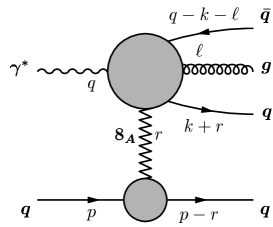
Figure 1: Kinematics of the process $\gamma^{*}+q^{\prime}\to q\bar{q}g+q^{\prime}$.

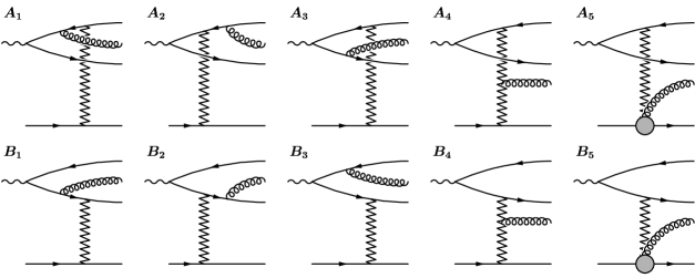
Figure 2: The diagrams contributing to $\Gamma_{{\gamma^{*}}\to q\bar{q}g}$

Fig.2 shows the Feynman diagrams. The product of two diagrams, summed over helicities and colors of the external particles, is labelled following the notation of the diagrams (e.g.: ${\cal A}{\cal B}_{12}=A_{1}B_{2}$). The expressions for the products ${\cal A}{\cal A}_{ij},{\cal A}{\cal B}_{ij},...$ that we use here are taken from real where, with one exception, we have used the same notation: in the present paper we combine, for the sake of simplification, the diagrams 4 and 5 in the product with diagram 4, i.e. we set:

$${\cal A}{\cal A}_{44} +{\cal A}{\cal A}_{45}+{\cal A}{\cal A}_{54}\,\longrightarrow{\cal A}{\cal A}_{44},$$

$${\cal A}{\cal A}_{45} ,{\cal A}{\cal A}_{54}\,\longrightarrow 0,$$

$${\cal A}{\cal B}_{44} +{\cal A}{\cal B}_{45}+{\cal A}{\cal B}_{54}\,\longrightarrow{\cal A}{\cal B}_{44},$$

$${\cal A}{\cal B}_{45} ,{\cal A}{\cal B}_{54}\,\longrightarrow 0,$$

and similarly for ${\cal B}{\cal A}$ and ${\cal B}{\cal B}$. All products ${\cal A}{\cal A}$ etc. have (transverse) dimension $-6$; in order to deal with dimensionless expressions we multiply with $(Q^{2})^{3}$. Let us introduce dimensionless variables:

$$\bm{k},\bm{\ell},\bm{r},\Lambda,\sqrt{s_{0}}\,\rightarrow\,\frac{1}{|Q|}(\bm{k},\bm{\ell},\bm{r},\Lambda,\sqrt{s_{0}})$$ (1)

(the meaning of $\Lambda$ and $s_{0}$ will become clear in a moment). From now on we will use only these new variables. We also define the abbreviations

$$\alpha_{1} \equiv\alpha\;,$$

$$\bar{\alpha}_{1} \equiv(1-\alpha-\alpha_{\ell})\;,$$

$$\alpha_{2} \equiv(1-\alpha)\;,$$

$$\bar{\alpha}_{2} \equiv(\alpha+\alpha_{\ell}).$$

Furthermore, we introduce the label ${\mathcal{A}\!\!\mathcal{B}}$, in order to denote a generic product of amplitudes (${\cal A}{\cal A},{\cal A}{\cal B},{\cal B}{\cal A}$ or ${\cal B}{\cal B}$):

$${\mathcal{A}\!\!\mathcal{B}} =\frac{(Q^{2})^{3}}{\alpha_{1}\bar{\alpha}_{1}}({\cal A}{\cal A}_{11}\;\mbox{or}\;{\cal A}{\cal A}_{12}\;\mbox{or}\;{\cal A}{\cal A}_{21}\,\ldots\,\mbox{or}\;{\cal A}{\cal B}_{11}.\ldots).$$ (2)

It is then easy to see that these ${\mathcal{A}\!\!\mathcal{B}}$’s are dimensionless and only depend on the dimensionless momenta $\bm{k},\bm{\ell}$ and $\bm{r}$. In (2) we have included a part of the $q\bar{q}g$ phase space measure in the definition of the ${\mathcal{A}\!\!\mathcal{B}}$’s, in order to simplify the expressions below. Finally, $|\Gamma^{(0)}_{\gamma^{*}\to q{\bar{q}}g}|^{2}$ will be proportional to the sum of all the ${\mathcal{A}\!\!\mathcal{B}}$.

The procedure of arriving at finite NLO corrections to the ${\gamma^{*}}$ impact factor has been described in combine . Let us briefly review the main steps. $|\Gamma^{(0)}_{\gamma^{*}\to q{\bar{q}}g}|^{2}$ has to be integrated over the $q\bar{q}g$ phase space. Before doing this integration, two restrictions have to be observed. First, we have to exclude that region of phase space where the gluon is separated in rapidity from the $q\bar{q}$ pair (central region); this configuration belongs to the LLA and has to be subtracted. To divide the $q\bar{q}g$ phase space an energy cutoff $s_{0}$ is introduced. This energy cutoff plays the role of the energy scale: when combining the NLO impact factor with the NLO BFKL Green function it will be important to use the same scale in all pieces. Since the virtual corrections to the NLO impact factor are independent of $s_{0}$, all dependence on the energy scale resides in the real corrections. As a result, the calculations described in this paper can already be used to study the $s_{0}$ dependence of the NLO impact factor. Next, we need to take care of the infrared infinities. The divergences in $|\Gamma^{(0)}_{\gamma^{*}\to q{\bar{q}}g}|^{2}$ due to the gluon being either soft or collinear to either of the fermions are regularised by subtracting the approximation of the squared vertex in the corresponding limit. These expressions are then re-added and integrated in $D=4-2\epsilon$ space-time dimensions, giving rise to poles in $\epsilon$, which drop out in combination with the virtual corrections and to finite pieces. The subtraction of the collinear limit requires the introduction of a momentum cutoff parameter, $\Lambda$. The final NLO corrections must be independent of this auxiliary parameter. In our numerical analysis we will perform this important test.

According to combine the full NLO corrections to the ${\gamma^{*}}$ impact factor have the following form:

$$\Phi_{{\gamma^{*}}}^{(1)}= \left.\Phi_{{\gamma^{*}}}^{(1,{\mathrm{v}irtual})}\right|^{\mathrm{f}inite}-\frac{2\Phi_{{\gamma^{*}}}^{(0)}}{(4\pi)^{2}}\left\{\beta_{0}\ln\frac{\bm{r}^{2}}{\mu^{2}}+C_{F}\ln(\bm{r}^{2})\right\}$$

$$+\int_{0}^{1}d\alpha\,\int\,\frac{d^{2-2\epsilon}\bm{k}}{(4\pi)^{2}}\,{\mathcal{I}}_{2}(\alpha,\bm{k})\,\bigg{\{}C_{A}\left[\ln^{2}\alpha(1-\alpha)s_{0}-\ln^{2}M^{2}\right]$$

$$\qquad\qquad+2C_{F}\left[8-3\ln\alpha(1-\alpha)\Lambda^{2}+\ln^{2}M^{2}+\ln^{2}\frac{\alpha}{1-\alpha}\right]\bigg{\}}$$

$$+C_{A}\left.\Phi_{{\gamma^{*}}}^{(1,{\mathrm{r}eal})}\right|_{C_{A}}^{\mathrm{f}inite}+C_{F}\left.\Phi_{{\gamma^{*}}}^{(1,{\mathrm{r}eal})}\right|_{C_{F}}^{\mathrm{f}inite}\;.$$ (3)

The terms multiplying $\Phi_{\gamma^{*}}^{(0)}$ stem from the UV renormalisation which belongs to the virtual corrections and does not need to be discussed in the present context. The finite pieces which are left after combining the IR singular pieces of the virtual and real corrections above are given in the second and third lines of eq.(II). ${\mathcal{I}}_{2}$ is proportional to the squared LO photon wave function:

$${\cal I}_{2}(\alpha,\bm{k})=\frac{2e^{2}e_{f}^{2}\sqrt{N_{c}^{2}-1}}{(2\pi)^{3-2\epsilon}(Q^{2})^{2\epsilon}}\alpha^{2}(1-\alpha)^{2}\left(\frac{1}{D(\bm{k})}-\frac{1}{D(\bm{k}+\bm{r})}\right)^{2}$$ (4)

with $D(\bm{k})=\bm{k}^{2}+\alpha(1-\alpha)$. Finally, the squared mass of the quark-antiquark pair, $M^{2}$, is a function of $\alpha,\bm{k},\bm{r}$, and it is not important for our present analysis.

Let us now focus on the last line of eq.(II). In terms of the products of single diagrams, ${\mathcal{A}\!\!\mathcal{B}}$, these finite contributions to the real corrections combine read:

$$\left.C_{F}\>\Phi_{{\gamma^{*}}}^{(1,{\mathrm{r}eal})}\right|_{C_{F}}^{\mathrm{f}inite}=\frac{e^{2}e_{f}^{2}\sqrt{N_{c}^{2}-1}}{(2\pi)^{6-4\epsilon}(Q^{2})^{2\epsilon}}\int d^{2-2\epsilon}\bm{k}\,d^{2-2\epsilon}\bm{\ell}\int_{0}^{1}d\alpha\int_{0}^{1-\alpha}\frac{d\alpha_{\ell}}{\alpha_{\ell}}\,$$

$$\hskip 19.91684pt\times\sum_{C_{F}}\Biggl{\{}{\mathcal{A}\!\!\mathcal{B}}-{\mathcal{A}\!\!\mathcal{B}}_{\mathrm{soft}}-\left({\mathcal{A}\!\!\mathcal{B}}_{\bar{\mathrm{q}}}-{\mathcal{A}\!\!\mathcal{B}}_{\bar{\mathrm{q}},\,soft}\right)\Theta(\alpha_{\ell}\Lambda-|\bm{\ell}^{\prime}|)$$

$${}\hskip 51.21504pt-\left({\mathcal{A}\!\!\mathcal{B}}_{\mathrm{q}}-{\mathcal{A}\!\!\mathcal{B}}_{{\mathrm{q}},\,soft}\right)\Theta(\alpha_{\ell}\Lambda-|\bm{\ell}\,^{\prime\prime}|)\Bigg{\}},$$ (5)

$$\left.C_{A}\>\Phi_{{\gamma^{*}}}^{(1,{\mathrm{r}eal})}\right|_{C_{A}}^{\mathrm{f}inite} =\frac{e^{2}e_{f}^{2}\sqrt{N_{c}^{2}-1}}{(2\pi)^{6-4\epsilon}(Q^{2})^{2\epsilon}}\int d^{2-2\epsilon}\bm{k}\,d^{2-2\epsilon}\bm{\ell}\int_{0}^{1}d\alpha\Bigg{\{}\int_{0}^{1-\alpha}\frac{d\alpha_{\ell}}{\alpha_{\ell}}$$

$$\times\sum_{C_{A}}\bigg{[}{\mathcal{A}\!\!\mathcal{B}}-{\mathcal{A}\!\!\mathcal{B}}_{\mathrm{soft}}-\left({\mathcal{A}\!\!\mathcal{B}}_{\mathrm{cen}}-{\mathcal{A}\!\!\mathcal{B}}_{\mathrm{cen,\,soft}}\right)\Theta(|\bm{\ell}|-\alpha_{\ell}\sqrt{s_{0}})\bigg{]}$$

$$- \int_{1-\alpha}^{\infty}\frac{d\alpha_{\ell}}{\alpha_{\ell}}\,\sum_{C_{A}}{\mathcal{A}\!\!\mathcal{B}}_{\mathrm{cen}}\,\Theta(|\bm{\ell}|-\alpha_{\ell}\sqrt{s_{0}})\Bigg{\}}.$$ (6)

The evaluation of these two expressions is the issue of this paper. The sums extend over the $C_{F}$ and $C_{A}$ parts of the ${\mathcal{A}\!\!\mathcal{B}}$’s, respectively. Note that the sum over all ${\mathcal{A}\!\!\mathcal{B}}$’s is essentially $|\Gamma^{(0)}_{\gamma^{*}\to q{\bar{q}}g}|^{2}$. Whereas the full sum is finite, the individual contributions ${\mathcal{A}\!\!\mathcal{B}}$’s, without further modifications, would be divergent: our task, therefore is to render them finite, diagram by diagram. This is the content of eqs.(II) and (II). In order to indicate the different limits where the integral of ${\mathcal{A}\!\!\mathcal{B}}$ diverges we use the following subscripts:

$$\mathrm{soft} :=\;\alpha_{\ell}\sim|\bm{\ell}|\to 0$$

$$\mathrm{\bar{q}} :=\;|\bm{\ell}^{\prime}|\to 0$$

$$\mathrm{q} :=\;|\bm{\ell}^{\prime\prime}|\to 0$$

$$\mathrm{cen} :=\;\alpha_{\ell}\to 0$$

$${\mathcal{A}\!\!\mathcal{B}}_{\mathrm{x,\,soft}} :=\left[{\mathcal{A}\!\!\mathcal{B}}_{\mathrm{x}}\right]_{\mathrm{soft}}.$$ (7)

Here $\bm{\ell}^{\prime}$ $\bm{\ell}\,^{\prime\prime}$ denote the two collinear vectors

$$\bm{\ell}^{\prime}=\bm{\ell}+\frac{\alpha_{\ell}}{\alpha_{2}}\bm{k}\quad,\quad\bm{\ell}\,^{\prime\prime}=\bm{\ell}-\frac{\alpha_{\ell}}{\alpha_{1}}\bm{(}\bm{k}+\bm{r}).$$ (8)

The parameter $\Lambda$ defines a cone around the collinear directions, specifying thereby the region of the subtraction. The exclusion of the central configuration (cen) is realised by subtraction: only the rapidity region $\alpha_{\ell}>|\bm{\ell}|/\sqrt{s_{0}}$ is counted as a contribution to the impact factor.

III The Integration

Our aim is, in eqs.(II,II), the analytic integration over $\bm{k}$ and $\bm{\ell}$. To this end we introduce Feynman parameters. Since different Feynman diagrams provide different denominators, we have to deal the ${\mathcal{A}\!\!\mathcal{B}}$’s independently rather than in the sum of all (as an alternative, an attempt the find common denominators would lead to expressions that have too lengthy numerators). As indicated in eqs.(II,II), in each single diagram ${\mathcal{A}\!\!\mathcal{B}}$ we have to combine the full expression with subtractions which are obtained from certain approximations (soft, cen,…), given by eq.(II). As a first step, we analyse the divergences of all diagrams. The table 1 shows, which diagram diverges in which limit. Both in the left hand and in the right hand part of the table, it is the second column which lists the divergent limits which in eqs.(II,II) require a suitable subtraction. The third columns contain an additional divergence that appears due to the separate treatment of the diagrams; we shall take care of them by making a further appropriate subtraction form each ${\mathcal{A}\!\!\mathcal{B}}$.

${\cal A}{\cal A}$			cen	cen/soft	soft	coll	l-uv	is	lr
11	$C_{F}$						$\times$
12	$C_{F}$,	$C_{A}$				$\bar{q}$	$\times$
22	$C_{F}$					$\bar{q}$	$\times$
13	$C_{F}$					$q$
23	$C_{F}$,	$C_{A}$			$\times$	$q,\,\bar{q}$
33	$C_{F}$					$q$
34		$C_{A}$				$q$
15		$C_{A}$	$\times$	$\times$				$\times$	$\times$
25		$C_{A}$	$\times$	$\times$	$\times$	$\bar{q}$			$\times$
35		$C_{A}$			$\times$	$q$		$\times$
14		$C_{A}$	$\times$				$\times$		$\times$
24		$C_{A}$	$\times$			$\bar{q}$	$\times$		$\times$
44		$C_{A}$	$\times$				$\times$		$\times$

${\cal A}{\cal B}$			cen	cen/soft	soft	coll	l-uv	is	lr
11	$C_{F}$,	$C_{A}$
12	$C_{F}$					$q$
22	$C_{F}$,	$C_{A}$			$\times$	$q,\,\bar{q}$
13	$C_{F}$,	$C_{A}$				$\bar{q}$
23	$C_{F}$					$\bar{q}$
33	$C_{F}$,	$C_{A}$			$\times$	$q,\,\bar{q}$
34		$C_{A}$				$q$
15		$C_{A}$	$\times$	$\times$				$\times$	$\times$
25		$C_{A}$	$\times$	$\times$	$\times$	$\bar{q}$			$\times$
35		$C_{A}$			$\times$	$q$		$\times$
14		$C_{A}$	$\times$						$\times$
24		$C_{A}$	$\times$			$\bar{q}$			$\times$
44		$C_{A}$	$\times$						$\times$

Table 1: The divergences of the diagrams ${\cal A}{\cal A}_{ij}$ and ${\cal A}{\cal B}_{ij}$

Let us go through these subtractions in some detail. Each product ${\mathcal{A}\!\!\mathcal{B}}$ has the general structure

$${\mathcal{A}\!\!\mathcal{B}}=\frac{Z}{D_{i}D_{j}D_{k}D_{l}}\quad,\qquad D_{n}=D_{n}(\bm{k},\bm{\ell},\bm{r}).$$ (9)

The denominators $D_{n}$ are given by (here we use definitions which slightly differ from those of real ):

$$D_{1} =\,\alpha_{\ell}\left[\alpha_{1}{\bar{\alpha}}_{1}+\alpha_{1}(\bm{k}+\bm{\ell}+\bm{r})^{2}+{\bar{\alpha}}_{1}(\bm{k}+\bm{r})^{2}\right]+\alpha_{1}{\bar{\alpha}}_{1}\bm{\ell}^{2}$$ (10)

$$D_{2} =\,\alpha_{1}\alpha_{2}+(\bm{k}+\bm{r})^{2}$$ (11)

$$D_{3} =(\alpha_{1}\,\bm{\ell}-\alpha_{\ell}\,(\bm{k}+\bm{r}))^{2}\,=\alpha_{1}^{2}\,\bm{\ell}^{{}^{\prime\prime}2}$$ (12)

$$D_{4} =(\bar{\alpha}_{1}\,\bm{\ell}+\alpha_{\ell}\,(\bm{k}+\bm{\ell}))^{2}\,=\alpha_{2}^{2}\,\bm{\ell}^{{}^{\prime}2}$$ (13)

$$D_{5} =\,\alpha_{\ell}\left(\alpha_{1}{\bar{\alpha}}_{1}+\alpha_{1}(\bm{k}+\bm{\ell})^{2}+{\bar{\alpha}}_{1}(\bm{k}+\bm{r})^{2}\right)+\alpha_{1}{\bar{\alpha}}_{1}(\bm{\ell}-\bm{r})^{2}$$ (14)

$$D_{6} =\alpha_{\ell}\left[\alpha_{1}{\bar{\alpha}}_{1}\,+{\bar{\alpha}}_{1}\bm{k}^{2}+\alpha_{1}\,(\bm{k}+\bm{\ell})^{2}\right]+\alpha_{1}{\bar{\alpha}}_{1}\,\bm{\ell}^{2}$$ (15)

$$D_{7} ={\bar{\alpha}}_{1}{\bar{\alpha}}_{2}\,+(\bm{k}+\bm{\ell})^{2}\;.$$ (16)

Note that, in some of the ${\mathcal{A}\!\!\mathcal{B}}$’s, two of the four $D^{\prime}s$ in eq.(9) may coincide. The numerator $Z$ is a polynomial in scalar products of the (dimensionless) transverse momenta:

$$Z=\lambda_{1}\,\bm{k}^{2}+\lambda_{2}\,\bm{\ell}^{2}+\lambda_{3}\,\bm{k}\bm{\ell}+\lambda_{4}\,\bm{k}\bm{r}+\lambda_{5}\,\bm{\ell}\bm{r}+\lambda_{6}\,\bm{r}^{2}+\lambda_{7}\>,\quad\lambda_{i}=\lambda_{i}(\alpha,\alpha_{\ell}).$$ (17)

(without our choice of dimensionless momenta, (1), the last term, $\lambda_{7}$, would have been proportional to $Q^{2}$). Let us now consider one single ${\mathcal{A}\!\!\mathcal{B}}$. Using

$$\prod_{i=1}\frac{1}{D_{i}^{p_{i}}}=\frac{\Gamma(\sum_{i}p_{i})}{\prod_{i}\Gamma(p_{i})}\;\int_{0}^{1}\prod_{i}\left(d\beta_{i}\,\beta_{i}^{p_{i}-1}\right)\,\frac{\delta(1-\sum_{i}\beta_{i})}{\left[\sum_{i}\beta_{i}D_{i}\right]^{\sum_{i}p_{i}}}.$$

we introduce the Feynman parameter representation:

$${\mathcal{A}\!\!\mathcal{B}}=6\int_{0}^{1}\; \prod_{i}d\beta_{i}\;\delta(1-\sum\beta_{i})\;f_{\beta}\>\>\frac{Z}{\left[\sum\beta_{i}D_{i}\right]^{4}}.$$ (18)

The $\beta_{i}$ carry the same labels as the denominators $D_{i}$ they belong to, and the sum in the denominator of (18) is understood to extend over those indices that occur in the diagram. $f_{\beta}$ stands for products and powers of the $\beta^{\prime}s$ in the numerator which appear in case of some of the four $D^{\prime}s$ being equal. For example, the product ${\cal A}{\cal B}_{13}$ reads

$$\frac{Z}{D_{1}^{2}\,D_{2}\,D_{3}}=6\int_{0}^{1}d\beta_{1}\,d\beta_{2}\,d\beta_{3}\;\frac{\delta(1-\sum\beta_{i})\>\beta_{1}\;Z}{\left[\beta_{1}D_{1}+\beta_{2}D_{2}+\beta_{3}D_{3}\right]^{4}}.$$ (19)

In order to determine the Feynman representation of the approximations of ${\mathcal{A}\!\!\mathcal{B}}$, we first consider the numerator and the denominator, in eq.(9), in the appropriate approximation; we denote the result by a subscript. Then, the Feynman representation is introduced as just described:

$${\mathcal{A}\!\!\mathcal{B}}_{x}=6\int_{0}^{1}\; \prod_{i}d\beta_{i}\;\delta(1-\mbox{$\sum$}\beta_{i})\>f_{\beta}\>\>\frac{Z|_{x}}{\left[\mbox{$\sum$}\beta_{i}\left.D_{i}\right|_{x}\right]^{4}}\>,\quad x=\mbox{$q$, $\bar{q}$, cen, ...}$$ (20)

Each limit in the original momentum space representation (in the $\{\bm{k},\bm{\ell},\alpha_{\ell}\}$ space) unambiguously corresponds to a ‘corner’ in the $\{\bm{k},\bm{\ell},\alpha_{\ell},\beta_{i}\}$ space of the Feynman parameter representation. By our way of calculating the Feynman representation of ${\mathcal{A}\!\!\mathcal{B}}_{\mathrm{soft}},{\mathcal{A}\!\!\mathcal{B}}_{\mathrm{q}},{\mathcal{A}\!\!\mathcal{B}}_{\mathrm{\bar{q}}},\ldots$, (20), we ensure that the cancellation between ${\mathcal{A}\!\!\mathcal{B}}$ and its approximations, which originally was formulated in the momentum space Feynman amplitudes, remains valid also after the introduction of Feynman parameters. The prescription (20) in particular ensures that our original expressions for the real corrections, eqs.(II, II), are exactly translated into the Feynman parameter space.

We now perform the integrations over $\bm{k}$ and $\bm{\ell}$. According to the different integration regions that occur in eqs.(II,II) we are faced with three different types of integrals. Let us discuss them in some detail. For convenience, we generalize to $2-2\epsilon$ transverse dimensions.

$\bullet\quad\int\>{\mathcal{A}\!\!\mathcal{B}}$

Let us consider the integration $\int d^{2-2\epsilon}\bm{k}\;d^{2-2\epsilon}\bm{\ell}\hskip 2.84544pt{\mathcal{A}\!\!\mathcal{B}}$. The $\bm{\ell}$-integration extends over the whole space. After the introduction of Feynman parameters, eq.(18), we have to integrate

$$J_{1}:=\int d^{2-2\epsilon}\bm{k}\;d^{2-2\epsilon}\bm{\ell}\>\frac{Z}{\left[\sum\beta_{i}D_{i}\right]^{4}}.$$ (21)

The generic structure of transverse momenta is:

$$J_{1}=\int d^{2-2\epsilon}\bm{k}\;d^{2-2\epsilon}\bm{\ell}\>\frac{\lambda_{1}\,\bm{k}^{2}+\lambda_{2}\,\bm{\ell}^{2}+\lambda_{3}\,\bm{k}\bm{\ell}+\lambda_{4}\,\bm{k}\bm{r}+\lambda_{5}\,\bm{\ell}\bm{r}+\lambda_{6}\,\bm{r}^{2}+\lambda_{7}}{\left[\tau\,\bm{k}^{2}+\rho\,\bm{\ell}^{2}+2\,\gamma\,\bm{k}\bm{\ell}+2\eta\,\bm{k}\bm{r}+2\mu\,\bm{\ell}\bm{r}+D_{r}\right]^{4}}.$$ (22)

The coefficients $\lambda_{i}$ in the numerator depend upon $\alpha,\alpha_{\ell}$. The coefficients in the denominator, $\tau,\rho,\gamma,...$, are functions of $\alpha,\alpha_{\ell}$ and of the Feynman parameters $\beta_{i}$. $D_{r}$ depends, in addition, on $\bm{r}^{2}$ (and on $Q^{2}$, which has been normalized to $1$). In order to eliminate, in the denominator, the mixed scalar products, we perform the shifts:

$$\bm{k} =\bm{k}^{\prime}-\frac{\gamma}{\tau}\bm{\ell}^{\prime}-\frac{1}{\mbox{det}\Omega}(\rho\eta-\gamma\mu)\bm{r}$$

$$\bm{\ell} =\bm{\ell}^{\prime}-\frac{1}{\mbox{det}\Omega}(\tau\mu-\gamma\eta)\bm{r}.$$ (23)

We arrive at:

$$J_{1}= \int d^{2-2\epsilon}\bm{k}^{\prime}\;d^{2-2\epsilon}\bm{\ell}^{\prime}\;\frac{A\,\bm{k}^{{}^{\prime}2}+B\,\bm{\ell}^{{}^{\prime}2}+C}{[\tau\bm{k}^{{}^{\prime}2}+\omega\bm{\ell}^{{}^{\prime}2}+R]^{4}},$$ (24)

where we have introduced the definitions

$$\omega=\frac{1}{\tau}\,\mbox{det}\Omega\>,\quad R=D_{r}-\frac{1}{\mbox{det}\Omega}(\eta^{2}\rho+\tau\mu^{2}-\eta\mu\gamma)\bm{r}^{2}\>,\quad\Omega=\left(\begin{array}[]{cc}\tau&\gamma\\ \gamma&\rho\end{array}\right).$$ (25)

In the numerator of (24) we have already dropped the mixed scalar products $(\bm{k}^{\prime}\,\bm{\ell}^{\prime},\bm{k}^{\prime}\,\bm{r}^{\prime},\bm{\ell}^{\prime}\,\bm{r}^{\prime})$: when performing, in (22), the shifts, such scalar products appear. However, after angular integration their contribution vanishes. Note that except for $A=\lambda_{1}$ all coefficient functions appearing in eq.(24), in general, depend on the Feynman parameters $\beta_{i}$ and on $\alpha,\alpha_{\ell}$. Performing the momentum integrations we get:

$$J_{1}= \int d^{2-2\epsilon}\bm{k}\;d^{2-2\epsilon}\bm{\ell}\;\frac{A\,\bm{k}^{2}+B\,\bm{\ell}^{2}+C}{[\tau\bm{k}^{2}+\omega\bm{\ell}^{2}+R]^{4}}$$

$$= \,\frac{\pi^{2-2\epsilon}}{6\,(\tau\omega)^{1-\epsilon}R^{1+2\epsilon}}\,\Bigg{\{}(1-\epsilon)\Gamma(1-2\epsilon)\,\left(\frac{A}{\tau}\;+\;\frac{B}{\omega}\right)\,+\Gamma(2+2\epsilon)\frac{C}{R}\,\Bigg{\}}.$$ (26)

Note that the integral converges for $\epsilon=0$. We will need the general result ($\epsilon\neq 0$) later. As our final result for the Feynman parameter representation of ${\mathcal{A}\!\!\mathcal{B}}$ we define a quantity $X$ by

$$\int d^{2}\bm{k}\;d^{2}\bm{\ell}\>{\mathcal{A}\!\!\mathcal{B}} =6\int_{0}^{1}\;\prod_{i}d\beta_{i}\;\delta(1-\mbox{$\sum\beta_{i}$})\>\,f_{\beta}\>\left.J_{1}\right|_{\epsilon=0}$$

$$=\int\prod_{i}d\beta_{i}\;\delta(1-\mbox{$\sum\beta_{i}$})\>\;X.$$ (27)

For each diagram ${\mathcal{A}\!\!\mathcal{B}}$, the function $X$ is given as MATHEMATICA code, described in the appendix.

In order to integrate the soft ($\bm{\ell}\sim\alpha_{\ell}\to 0$) approximation of ${\mathcal{A}\!\!\mathcal{B}}$ we consider the numerator and the denominator of ${\mathcal{A}\!\!\mathcal{B}}$ in the soft approximation and introduce the Feynman parameter representation according to (20). We then carry out the momentum integration exactly as just described ending up with an expression which we call $X_{\mathrm{soft}}$:

$$\int d^{2}\bm{k}\;d^{2}\bm{\ell}\>{\mathcal{A}\!\!\mathcal{B}}_{\mathrm{soft}} =6\int\;\prod_{i}d\beta_{i}\;\delta(1-\mbox{$\sum$}\beta_{i})\>\int d^{2}\bm{k}\;d^{2}\bm{\ell}\frac{f_{\beta}\>Z|_{\mathrm{soft}}}{\left[\mbox{$\sum$}\beta_{i}\left.D_{i}\right|_{\mathrm{soft}}\right]^{4}}$$

$$=\int\prod_{i}d\beta_{i}\;\delta(1-\mbox{$\sum\beta_{i}$})\>\;X_{\mathrm{soft}}.$$ (28)

It is instructive to see how the soft limit in the momentum space translates into the Feynman parameter space. The corresponding region in the Feynman parameters space is determined by the behaviour of the denominators $D_{i}$ in the soft limit. One obtains $\sum\beta_{i}D_{i}|_{\mathrm{soft}}$ from $\sum\beta_{i}D_{i}$ by ‘weighting’ $\{\beta_{2},\beta_{5},\beta_{7}\}\to\{\beta_{2},\beta_{5},\beta_{7}\}\rho^{2}$, $\{\beta_{1},\beta_{6},\bm{\ell},\alpha_{\ell}\}\to\{\beta_{1},\beta_{6},\bm{\ell},\alpha_{\ell}\}\rho$, and then expanding around $\rho=0$ and by keeping only the most divergent term. The prescription for the $\beta$’s remains unchanged after the integration over $\bm{\ell}$ and $\bm{k}$; the soft region is therefore specified by:

$$\mathrm{soft:}\qquad\beta_{2},\beta_{5},\beta_{7}\quad\ll\quad\beta_{1},\beta_{6},\alpha_{\ell}\quad\ll\quad\beta_{3},\beta_{4}.$$ (29)

Hence, we can obtain $X_{\mathrm{soft}}$ either in the way given in eq.(III) or by considering $X$ (eq.(III)) in the limit (29) (indicated by the subscript):

$$\int d^{2}\bm{k}\;d^{2}\bm{\ell}\>{\mathcal{A}\!\!\mathcal{B}}_{\mathrm{soft}}$$

$$=6\int\;\prod_{i}d\beta_{i}\;\delta(1-\mbox{$\sum$}\beta_{i})\>\int d^{2}\bm{k}\;d^{2}\bm{\ell}\left[\frac{f_{\beta}\;Z}{\left[\mbox{$\sum$}\beta_{i}D_{i}\right]^{4}}\right]_{\textstyle\beta_{2},\beta_{5},\beta_{7}\ll\beta_{1},\beta_{6},\alpha_{\ell},\bm{\ell}\ll\beta_{3},\beta_{4}}$$

$$=\int\prod_{i}d\beta_{i}\;\delta(1-\mbox{$\sum$}\beta_{i})\>\;\left[X\right]_{\eqref{eq:softlimit}}$$ (30)

Note that we must not apply the approximation (29) to the argument $\delta$-function in eq.(30) (otherwise, the translation of the real corrections from the momentum space to the Feynman parameter space would be incorrect). This has the following consequence. After choosing any of the $\beta$-integrations to be done by means of the $\delta$-function we have

$$\int d\beta_{k}\prod_{i}d\beta_{i}\;\delta(1-\mbox{$\sum\beta_{i}$})\>\left(X-X_{\mathrm{soft}}\right)=\int\prod_{i}d\beta_{i}\;\>\left(\tilde{X}-\tilde{X}_{\mathrm{soft}}\right)$$ (31)

with the tilde symbol on the rhs indicating that $\beta_{k}$ is expressed in terms of the other $\beta_{i}$. Since the argument of the $\delta$-function is not approximated, $\tilde{X}_{\mathrm{soft}}$ is not equal to $\tilde{X}$ taken in the limit (29). However, both $\tilde{X}_{\mathrm{soft}}$ and $\tilde{X}$ become equal in this limit.

$\bullet\quad\int^{\Lambda}{\mathcal{A}\!\!\mathcal{B}}_{\mathrm{coll}}$

Next we turn to the collinear approximation of ${\mathcal{A}\!\!\mathcal{B}}$. We use the label ’coll’ to denote the two collinear limits which are defined as either $|\bm{\ell}^{\prime\prime}|\to 0$ or $|\bm{\ell}^{\prime}|\to 0$ (cf. eqs.(II) and (8)). Following the notation introduced in eq.(20) we use the collinear approximation of the numerator of ${\mathcal{A}\!\!\mathcal{B}}$ and of the $D^{\prime}s$. The region of integration is restricted to a cone around the collinear direction:

$$J_{2}:=\int d^{2-2\epsilon}\bm{k}\;d^{2-2\epsilon}\bm{\ell}\>\>\Theta(\alpha_{\ell}\Lambda-|\bm{\ell}_{c}|)\>\>\frac{Z_{\mathrm{coll}}}{\left[\sum\beta_{i}\left.D_{i}\right|_{\mathrm{coll}}\right]^{4}}\>,\>\quad\bm{\ell}_{c}=\bm{\ell}^{\prime},\bm{\ell}^{\prime\prime}.$$ (32)

Starting from eq.(32) we first express $\bm{\ell}$ in eq.(32) through $\bm{\ell}_{c}$. The list of the $D^{\prime}s$ in eqs.(10) - (16) shows that in the limit $\bm{\ell}^{\prime}\to 0$, in leading order, all $D_{i}$ become independent of $\bm{\ell}^{\prime}$, except for $D_{4}$ which is proportional to $\bm{\ell}^{{}^{\prime}2}$. The same holds for the the second collinear limit, with $D_{3}$ instead of $D_{4}$. The denominator in eq.(32) therefore depends on $\bm{\ell}_{c}$ only via $\bm{\ell}_{c}^{2}$ and the integrand is parametrised as

$$J_{2}=\int d^{2-2\epsilon}\bm{k}\; d^{2-2\epsilon}\bm{\ell}_{c}\>\Theta(\alpha_{\ell}\Lambda-|\bm{\ell}_{c}|)$$

$$\times\frac{\lambda_{1}\,\bm{k}^{2}+\lambda_{2}\,\bm{\ell}_{c}^{2}+\lambda_{3}\,\bm{k}\bm{\ell}_{c}+\lambda_{4}\,\bm{k}\bm{r}+\lambda_{5}\,\bm{\ell}_{c}\bm{r}+\lambda_{6}\,\bm{r}^{2}+\lambda_{7}}{\left[\tau\,\bm{k}^{2}+\rho\,\bm{\ell}_{c}^{2}+2\eta\,\bm{k}\bm{r}+D_{r}\right]^{4}}.$$ (33)

Note that, since we are using $\bm{\ell}_{c}$ instead of $\bm{\ell}$, the coefficients in eq.(III) are not the same as in eq.(22), taken in a collinear approximation. It is only for keeping the notation as simple as possible that we do not introduce new names for the coefficients. In order to diagonalise the denominator we only have to get rid of $\bm{k}\bm{r}$; the momentum $\bm{\ell}_{c}$, therefore, does not participate in the shift of momenta (III), and the limits of the $\bm{\ell}_{c}$ integration remain the same. Applying, to (III), the shift (III) with $\gamma=\mu=0$, we arrive at

$$J_{2}= \int d^{2}\bm{k}\;d^{2}\bm{\ell}\;\Theta(\alpha_{\ell}\Lambda-|\bm{\ell}|)\>\frac{A\,\bm{k}^{2}+B\,\bm{\ell}^{2}+C}{[\tau\bm{k}^{2}+\omega\bm{\ell}^{2}+R]^{4}}$$

$$= \;\frac{\pi^{2}\bar{\Lambda}^{2}}{6\,\tau\omega R(R+\bar{\Lambda}^{2})}\;\left[A\frac{1}{\tau}+B\frac{1}{\omega}\>\frac{\bar{\Lambda}^{2}}{R+\bar{\Lambda}^{2}}+C\frac{1}{R}\>\frac{2R+\bar{\Lambda}^{2}}{R+\bar{\Lambda}^{2}}\right]$$ (34)

$$\mbox{with :}\;\bar{\Lambda}^{2}=\omega(\alpha_{\ell}\Lambda)^{2}.$$

Below we will show that only the result for $\epsilon=0$ is needed. In analogy to eq.(III) we define $X_{\mathrm{coll}}$ to be $6f_{\beta}J_{2}$ after performing the integration over the transverse momenta:

$$\int d^{2}\bm{k}\;d^{2}\bm{\ell}\>{\mathcal{A}\!\!\mathcal{B}}_{\mathrm{coll}}\>\Theta(\alpha_{\ell}\Lambda-|\bm{\ell}_{c}|) =6\int_{0}^{1}\;\prod_{i}d\beta_{i}\;\delta(1-\mbox{$\sum\beta_{i}$})\>\,f_{\beta}\left.J_{2}\right|_{\epsilon=0}$$

$$=\int\prod_{i}d\beta_{i}\;\delta(1-\mbox{$\sum\beta_{i}$})\>\;X_{\mathrm{coll}}.$$ (35)

In the collinear limits all $D_{i}$, except $D_{4}$ ($D_{3}$), become independent of $\bm{\ell}_{c}$. In the $\beta_{i}$ space these limits therefore read:

$$\mathrm{coll}\;{\bar{q}}:\qquad \beta_{i\neq 4}\quad\ll\quad\beta_{4}$$ (36)

$$\mathrm{coll}\;q:\qquad \beta_{i\neq 3}\quad\ll\quad\beta_{3}.$$ (37)

However, in momentum space the integrals of ${\mathcal{A}\!\!\mathcal{B}}_{\mathrm{coll}}$ and ${\mathcal{A}\!\!\mathcal{B}}$ have different limits of integration. It turns out that, as a consequence, $X_{\mathrm{coll}}$, in the limit (36) or (37), can be written as a sum of two parts. The first one coincides with the collinear limit (either (36) or (37)) of $X$. The other term depends on $\Lambda$, and vanishes in the collinear limit (36) or (37).

Next we need to consider the soft limit of the collinear limit, the collinear-soft approximation ${\mathcal{A}\!\!\mathcal{B}}_{\mathrm{coll,soft}}$. In momentum space, this limit is calculated by taking, in ${\mathcal{A}\!\!\mathcal{B}}_{\mathrm{coll}}(\bm{k},\bm{\ell}_{c},\alpha_{\ell})$, the additional limit $\bm{\ell}_{c}\sim\alpha_{\ell}\to 0$ (cf. the definition of $\bm{\ell}_{c}$ in (8)). It is then integrated exactly in the same way as just described for $X_{\mathrm{coll}}$,

$$\int d^{2}\bm{k}\,d^{2}\bm{\ell}\;{\mathcal{A}\!\!\mathcal{B}}_{\mathrm{coll,soft}}\>\Theta(\alpha_{\ell}\Lambda-|\bm{\ell}_{c}|)=\int\mbox{$\prod$}\beta_{i}\;\delta(1-\mbox{$\sum\beta_{i}$})\>\;X_{\mathrm{coll,soft}}.$$ (38)

Turning to the collinear-soft limit in the $\beta_{i}$ space, one finds that the soft limits of the $D_{i}$ and of the $\left.D_{i}\right|_{\mathrm{coll}}$ coincide. However, the $\bm{\ell}_{c}$-integration of ${\mathcal{A}\!\!\mathcal{B}}_{\mathrm{coll,soft}}$ in (38), in contrast to the integral of ${\mathcal{A}\!\!\mathcal{B}}_{\mathrm{soft}}$, has an upper limit of integration. But one can show that due to the $\alpha_{\ell}$-dependence of the integration limit $\alpha_{\ell}\Lambda$ in eq.(38) the position of the soft limit in the $\{\alpha_{\ell},\beta_{i}\}$ subspace (of the $\{\bm{\ell}_{c},\alpha_{\ell},\beta_{i}\}$ space) is unchanged by the $\bm{\ell}_{c}$ integration. Also in case of the integration of ${\mathcal{A}\!\!\mathcal{B}}_{\mathrm{soft}}$ (without upper limit on $\bm{\ell}$) the soft region is unchanged by the $\bm{\ell}$ integration, see eq.(30). The soft limits of $X$ and $X_{\mathrm{coll}}$, therefore, are located in the same region of the $\beta_{i}$ space:

$$\mbox{soft of coll:}\qquad\beta_{2},\beta_{5},\beta_{7}\quad\ll\quad\beta_{1},\beta_{6},\alpha_{\ell}\quad\ll\quad\beta_{3},\beta_{4}.$$ (39)

$\bullet\quad\int_{s_{0}}{\mathcal{A}\!\!\mathcal{B}}_{\mathrm{cen}}$

The third type of integral appearing in the real corrections, eq.(II) and (II), deals with the central approximation ${\mathcal{A}\!\!\mathcal{B}}_{\mathrm{cen}}$, defined by the limit $\alpha_{\ell}\to 0$:

$$J_{3}:=\int d^{2-2\epsilon}\bm{k}\;d^{2-2\epsilon}\bm{\ell}\>\>\Theta(|\bm{\ell}|-\alpha_{\ell}s_{0})\>\>\frac{Z_{\mathrm{cen}}}{\left[\sum\beta_{i}\left.D_{i}\right|_{\mathrm{cen}}\right]^{4}}.$$ (40)

Its general form reads:

$$J_{3}=\int d^{2-2\epsilon}\bm{k}\; d^{2-2\epsilon}\bm{\ell}\>\>\Theta(|\bm{\ell}|-\alpha_{\ell}s_{0})\>\>$$

$$\times\frac{\lambda_{1}\,\bm{k}^{2}+\lambda_{2}\,\bm{\ell}^{2}+\lambda_{3}\,\bm{k}\bm{\ell}+\lambda_{4}\,\bm{k}\bm{r}+\lambda_{5}\,\bm{\ell}\bm{r}+\lambda_{6}\,\bm{r}^{2}+\lambda_{7}}{\left[\tau\,\bm{k}^{2}+\rho\,\bm{\ell}^{2}+2\,\gamma\,\bm{k}\bm{\ell}+2\eta\,\bm{k}\bm{r}+2\mu\,\bm{\ell}\bm{r}+D_{r}\right]^{4}}.$$ (41)

In order to keep the region of the $\bm{\ell}$-integration as simple as possible, we do not perform any shift in $\bm{\ell}$; this will leave us with angular dependent terms of the form $\bm{\ell}\bm{r}$, both in the numerator and in the denominator. We only perform the shift eq.(III) of $\bm{k}$, given by eq.(III), with $\bm{\ell}^{\prime}$ being expressed through $\bm{\ell}$ and $\bm{r}$:

$$\bm{k} =\bm{k}^{\prime}-\frac{\gamma}{\tau}(\bm{\ell}+\lambda\bm{r})-\frac{1}{\mbox{det}\Omega}\left(\rho\eta-\gamma\mu\right)\bm{r}\>,\quad\lambda=\frac{1}{\mbox{det}\Omega}(\tau\mu-\gamma\eta),$$ (42)

and we obtain

$$J_{3}= \int d^{2}\bm{k}\;d^{2}\bm{\ell}\>\Theta(|\bm{\ell}|-\alpha_{\ell}\sqrt{s_{0}})\>\frac{A\,\bm{k}^{2}+B\,\bm{\ell}^{2}+C+E\,\bm{\ell}\bm{r}}{[\tau\bm{k}^{2}+\omega(\bm{\ell}+\lambda\bm{r})^{2}+R]^{4}}$$

$$={} \frac{\pi^{2}}{6\tau\omega R}\;\left(\frac{A}{\tau}\;{\mathcal{C}}_{A}+\frac{B}{\omega}\;{\mathcal{C}}_{B}+\frac{C}{R}\;{\mathcal{C}}_{C}+\frac{E}{R}\lambda|\bm{r}|\;{\mathcal{C}}_{E}\right).$$ (43)

The coefficients $\omega$ and $R$ are given by eq.(25), expressed in terms of the coefficients in the denominator of eq.(III). Again, we only need the case $\epsilon=0$. The coefficients in the second line on the rhs of (III) are given by

$${\mathcal{C}}_{A} =\frac{1}{2}\left\{1-\frac{1}{\kappa}\Big{[}\bar{s}_{0}-(R+\bar{\bm{\lambda}}^{2})\Big{]}\right\}$$

$${\mathcal{C}}_{B} =\frac{1}{2}\left\{\frac{\bar{\bm{\lambda}}^{2}+R}{R}-\frac{1}{R\kappa}\,\Big{[}\bar{s}_{0}\,(R+\bar{\bm{\lambda}}^{2})-3R^{2}-\bar{\bm{\lambda}}^{4}\Big{]}\right.$$

$$\left.\hskip 28.45274pt-{}\frac{2}{\kappa^{3}}\,\Big{[}(R-\bar{\bm{\lambda}}^{2})(R+\bar{\bm{\lambda}}^{2})^{2}+\bar{s}_{0}\,(R^{2}+\bar{\bm{\lambda}}^{4}-6R\bar{\bm{\lambda}}^{2})\Big{]}\right\}$$

$${\mathcal{C}}_{C} =\frac{1}{2}\left\{1-\frac{1}{\kappa}\Big{[}\bar{s}_{0}+(R-\bar{\bm{\lambda}}^{2})\Big{]}+\frac{2R}{\kappa^{3}}\Big{[}\bar{s}_{0}\,(R-\bar{\bm{\lambda}}^{2})+(R+\bar{\bm{\lambda}}^{2})^{2}\Big{]}\right\}$$

$${\mathcal{C}}_{E} =-\frac{1}{2}\left\{1-\frac{1}{\kappa}\Big{[}\bar{s}_{0}+(R-\bar{\bm{\lambda}}^{2})\Big{]}+\frac{2R}{\kappa^{3}}\Big{[}\bar{s}_{0}\,(3R-\bar{\bm{\lambda}}^{2})+(R+\bar{\bm{\lambda}}^{2})^{2}\Big{]}\right\};$$ (44)

where we have defined :

$$\bar{s}_{0}\equiv\omega(\alpha_{\ell}\sqrt{s_{0}})^{2}\>,\qquad\bar{\bm{\lambda}}^{2}\equiv\omega\lambda^{2}\bm{r}^{2}$$

$$\mbox{and :}\quad\kappa\equiv\sqrt{\left(\bar{s}_{0}+R+\bar{\bm{\lambda}}^{2}\right)^{2}-4\bar{s}_{0}\,\bar{\bm{\lambda}}^{2}}.$$

In complete analogy to the previous integrations we finally define

$$\int d^{2}\bm{k}\,d^{2}\bm{\ell}\;{\mathcal{A}\!\!\mathcal{B}}_{\mathrm{cen}}\>\Theta(|\bm{\ell}|-\alpha_{\ell}\sqrt{s_{0}})=\int\mbox{$\prod$}\beta_{i}\;\delta(1-\mbox{$\sum\beta_{i}$})\>\;X_{\mathrm{cen}}.$$ (45)

Turning to the soft limit of the central-soft approximation, we again start in momentum space, introduce Feynman parameters, perform the momentum integration, and arrive at $X_{\mathrm{cen,soft}}$, in analogy to eq.(45). Due to the different limits of integration of ${\mathcal{A}\!\!\mathcal{B}}$ and ${\mathcal{A}\!\!\mathcal{B}}_{\mathrm{cen}}$, only a part of $X_{\mathrm{cen}}$ matches the central approximation of $X$, the rest depends on $s_{0}$ and vanishes in the central limit. Similar to the collinear approximation, the $\alpha_{\ell}$-dependence of the lower limit on the $\bm{\ell}$ integration (45) has the effect that the momentum integration does not change the position of the soft region in the $\{\alpha_{\ell},\beta_{i}\}$ space. The soft limit is located in the region:

$$\mbox{soft of cen:}\qquad\beta_{2},\beta_{5},\beta_{7}\quad\ll\quad\alpha_{\ell}\quad\ll\quad\beta_{1},\beta_{3},\beta_{4},\beta_{6}.$$ (46)

As we have mentioned before, when treating individual diagrams, ${\mathcal{A}\!\!\mathcal{B}}$, additional logarithmic divergences appear which do not show up in the sum. They occur in the following limits:

$$\bm{\ell}\!-\!\mathrm{uv}\; :\;|\bm{\ell}|\to\infty$$

is $$:\;|\bm{\ell}|\sim\sqrt{\alpha}_{\ell}\to 0$$

lr $$:\;\bm{\ell}\to\bm{r}.$$ (47)

Tab.1 contains, in the third columns, a list of those diagrams where these divergences appear. These divergences lead to additional subtractions which we have to describe in some detail. Let us start with the $C_{F}$ parts. They do not contribute to the central limit. The only additional divergence is of the type $\bm{\ell}\!-\!\mathrm{uv}$; in this limit, all denominators $D_{i}$ (10) - (16) are proportional to $\bm{\ell}^{2}$, except for $D_{2}$ which is independent of $\bm{\ell}$. Any ${\mathcal{A}\!\!\mathcal{B}}$ containing $D_{2}^{2}$ in the denominator and a term proportional to $\bm{\ell}^{2}$ in the numerator will therefore, in the limit $\bm{\ell}\to\infty$, be proportional to $1/\bm{\ell}^{2}$, leading to an UV divergent $\bm{\ell}$ integration. Subtracting from such diagram its approximation in this UV-limit, ${\mathcal{A}\!\!\mathcal{B}}_{\bm{\ell}\!-\!\mathrm{uv}}$, would cancel the $\bm{\ell}\!-\!\mathrm{uv}$ divergence. However, the $\bm{\ell}$ integration then becomes IR divergent instead, since ${\mathcal{A}\!\!\mathcal{B}}_{\bm{\ell}\!-\!\mathrm{uv}}\sim 1/\bm{\ell}^{2}$. We therefore define our subtraction term in the Feynman parameter space where it is easy to avoid this additional IR divergence. Let us demonstrate this at a simplified expression $A=1/[(c+\bm{\ell}^{2})D_{2}]$. $c$ is a constant and $D_{2}$ does not depend on $\bm{\ell}$. We introduce the Feynman representation and integrate over $\bm{\ell}$ (assuming already a term that cancels the $\bm{\ell}\!-\!\mathrm{uv}$ divergence):

$$\int_{0}^{\infty}d\bm{\ell}^{2}\>A=\int_{0}^{\infty}d\bm{\ell}^{2}\frac{1}{(c+\bm{\ell}^{2})D_{2}}=\int d\beta_{1}d\beta_{2}\int_{0}^{\infty}d\bm{\ell}^{2}\frac{\delta(1-\beta_{1}-\beta_{2})}{[\beta_{1}(\bm{\ell}^{2}+c)+\beta_{2}D_{2}]^{2}}$$

$$=\int d\beta_{1}d\beta_{2}\;\delta(1-\beta_{1}-\beta_{2})\>\frac{1}{\beta_{1}(\beta_{1}c+\beta_{2}D_{2})}=\int_{0}^{1}\frac{d\beta_{1}}{\beta_{1}(\beta_{1}(c-D_{2})+D_{2})}$$ (48)

The divergence at $\bm{\ell}\to\infty$ appears in the limit $\beta_{1}\to 0$ after the integration. The natural subtraction in the Feynman parameter space therefore reads

$$\int_{0}^{1}\left(\frac{d\beta_{1}}{\beta_{1}(\beta_{1}(c-D_{2})+D_{2})}-\frac{d\beta_{1}}{\beta_{1}D_{2}}\right).$$ (49)

As an alternative subtraction term we could use the $\bm{\ell}\!-\!\mathrm{uv}$ limit of $A$, which is $1/[\bm{\ell}^{2}D_{2}]$, in Feynman parameter representation. It is obtained by taking the integrand in the second line of eq.(III) in the limit $\beta_{1}\to 0$ excluding the argument of the $\delta$-function from this approximation. Carrying out the $\beta_{2}$ integration this results in

$$\frac{1}{\beta_{1}(1-\beta_{1})D_{2}}.$$

The additional divergence of this term at $\beta_{1}\to 1$ corresponds to the limit $\bm{\ell}\to 0$ in the momentum space and can be avoided by using the subtraction eq.(49).

We therefore regularise the $\bm{\ell}\!-\!\mathrm{uv}$ divergence of our diagrams in the following way. Due to the behaviour of the $D_{i}$’s in the $\bm{\ell}\!-\!\mathrm{uv}$ limit mentioned above, the region $\bm{\ell}\to\infty$ translates to the region $\beta_{i\neq 2}\ll\beta_{2}$ in the Feynman parameter space. Each $\bm{\ell}\!-\!\mathrm{uv}$ divergent diagram has a $D_{2}$ in the denominator. After the introduction of the Feynman representation and after carrying out the momentum integration we always perform the $\beta_{2}$ integration by means of the $\delta$-function in case of these diagrams. The subtraction term is then determined by taking the limit $\beta_{i\neq 2}\ll 1$ in $2-2\epsilon$ transverse dimensions:

$$\int d^{2-2\epsilon}\bm{k}\;d^{2-2\epsilon}\bm{\ell}\>{\mathcal{A}\!\!\mathcal{B}} =\int d\beta_{2}\,\prod_{i}d\beta_{i}\;\delta(1-\beta_{2}-\mbox{$\sum\beta_{i}$})\>\;X=\int\prod_{i}d\beta_{i}\;\tilde{X}$$

$$=\int\prod_{i}d\beta_{i}\;\left(\tilde{X}-\tilde{X}_{\mathrm{\bm{\ell}\!-\!\mathrm{uv}}}\right)+\int\prod_{i}d\beta_{i}\;\tilde{X}_{\mathrm{\bm{\ell}\!-\!\mathrm{uv}}},$$ (50)

$${}\qquad\mbox{with:}\quad\tilde{X}_{\mathrm{\bm{\ell}\!-\!\mathrm{uv}}}=\left.\tilde{X}\right|_{\beta_{i}\ll 1}$$

To perform the momentum integration we needed to calculate the integral in eq.(III) for $\epsilon\neq 0$. The tilde in eq.(III) indicates that $\beta_{2}$ in $X$ is expressed in terms of the other $\beta_{i}$. We perform the $\beta_{i}$ integration in the re-added piece analytically, obtaining an $\epsilon$-pole and finite terms. Summing up the re-added $\bm{\ell}\!-\!\mathrm{uv}$ subtractions from all diagrams we find that the poles cancel, as expected.

We can now write down the final result (after momentum integration) for the $C_{F}$ part of the real corrections (II). Using the definitions (III), (III), and (38) we obtain

$$\left.\Phi_{{\gamma^{*}}}^{(1,{\mathrm{r}eal})}\right|_{C_{F}}^{\mathrm{f}inite} =\frac{e^{2}e_{f}^{2}\sqrt{N_{c}^{2}-1}}{(2\pi)^{6}}\Bigg{\{}\sum_{C_{F}}\;\int_{0}^{1}d\alpha\int_{0}^{1-\alpha}\frac{d\alpha_{\ell}}{\alpha_{\ell}}\int_{0}^{1}\mbox{$\prod$}d\beta_{i}\>\delta(1-\mbox{$\sum$}\beta_{i})$$

$$\bigg{(}X-X_{\mathrm{soft}}-X_{\bm{\ell}\!-\!\mathrm{uv}}-(X_{q}-X_{q,\mathrm{soft}})-(X_{\bar{q}}-X_{{\bar{q}},\mathrm{soft}})\bigg{)}^{C_{F}}$$

$$+\frac{\pi^{2}}{24}\;(3\pi^{2}-28)\Bigg{\}}.$$ (51)

The superscript indicates that only the $C_{F}$ part of the bracket is taken, excluding the color factor $C_{F}$. To simplify notations, we have written the delta function $\delta(1-\mbox{$\sum$}\beta_{i})$ also for the $X_{\bm{\ell}\!-\!\mathrm{uv}}$ term. However, as discussed above, $\beta_{2}$ in $X_{\bm{\ell}\!-\!\mathrm{uv}}$ is understood to be already expressed in terms of the other $\beta_{i}$. We have set $\epsilon=0$ in (III) since the $\beta_{i}$ integrals are convergent by construction. This is why we needed to calculate the integrals over ${\mathcal{A}\!\!\mathcal{B}}_{\mathrm{coll}}$ and ${\mathcal{A}\!\!\mathcal{B}}_{\mathrm{cen}}$ only for the case $\epsilon=0$. The term in the third line of eq.(III) results from the sum of the re-added $\bm{\ell}\!-\!\mathrm{uv}$ subtractions.

Now we turn to the $C_{A}$ parts of the diagrams. We have to deal with collinear divergences. However, according to real the collinear approximations of all $C_{A}$ parts sum up to zero; we can therefore just subtract from the divergent ${\mathcal{A}\!\!\mathcal{B}}^{\prime}s$ their collinear approximation without re-adding it (as in the $C_{A}$ case, we restrict the integration to a cone since otherwise it would be UV divergent).

According to tab.1, in the $C_{A}$ parts we encounter all three types of additional divergences. As to the is(intersoft)-divergence, one finds in momentum space:

$$\sum_{C_{A}}\,({\mathcal{A}\!\!\mathcal{B}}-{\mathcal{A}\!\!\mathcal{B}}_{\mathrm{soft}})_{is}=0.$$

We can therefore regularise this divergence by subtracting, from $({\mathcal{A}\!\!\mathcal{B}}-{\mathcal{A}\!\!\mathcal{B}}_{\mathrm{soft}})$, its is-approximation, without re-adding it. In the appendix we provide the combinations $({\mathcal{A}\!\!\mathcal{B}}-{\mathcal{A}\!\!\mathcal{B}}_{\mathrm{soft}})_{is}$ in the $\beta_{i}$ space, $(X-X_{\mathrm{soft}})_{\mathrm{is}}$, which can be obtained from $X-X_{\mathrm{soft}}$ by taking the is-limit (before making use of the $\delta$-function):

$$\mathrm{is:}\qquad\beta_{2},\beta_{5},\beta_{7},\alpha_{\ell}\quad\ll\quad\beta_{1},\beta_{3},\beta_{4},\beta_{6}.$$ (52)

In the lr-limit ($\bm{\ell}\to\bm{r}$), it is the central approximation of certain diagrams that diverges. Let us recall the structure of the ${\cal A}{\cal A}$ and ${\cal A}{\cal B}$ diagrams in the central limit $\alpha_{\ell}\to 0$ (see real ):

$$\left.{\cal A}{\cal A}_{ij}\right|_{\mathrm{cen}} =\frac{\alpha_{1}^{3}\,\alpha_{2}^{3}\,C_{A}}{(\bm{\ell}-\bm{r})^{2}}\;\frac{1}{D^{2}(\bm{k}+\bm{r})}\;D_{ij}\;,$$ (53)

$$\left.{\cal A}{\cal B}_{ij}\right|_{\mathrm{cen}} =\frac{-\alpha_{1}^{3}\,\alpha_{2}^{3}\,C_{A}}{(\bm{\ell}-\bm{r})^{2}}\;\frac{1}{D(\bm{k}+\bm{r})D(\bm{k}+\bm{\ell})}\;D_{ij}\;.$$ (54)

where $D(\bm{k})=\alpha_{1}\alpha_{2}+\bm{k}^{2}$. The matrix $D_{ij}$ reads :

$$\begin{pmatrix}0&0&0&-\frac{1}{2}&\frac{\bm{r}^{2}}{\bm{\ell}^{2}}\\ 0&0&0&-\frac{1}{2}&\frac{\bm{r}^{2}}{\bm{\ell}^{2}}\\ 0&0&0&0&0\\ -\frac{1}{2}&-\frac{1}{2}&0&2&0\\ \frac{\bm{r}^{2}}{\bm{\ell}^{2}}&\frac{\bm{r}^{2}}{\bm{\ell}^{2}}&0&0&0\end{pmatrix}\;.$$

The denominators in eqs.(53) and (54) correspond to :

$$\left.D_{2}\right|_{\mathrm{cen}} =D(\bm{k}+\bm{r})$$

$$\left.D_{5}\right|_{\mathrm{cen}} =\alpha_{1}\alpha_{2}(\bm{\ell}-\bm{r})^{2}$$ (55)

$$\left.D_{7}\right|_{\mathrm{cen}} =D(\bm{k}+\bm{\ell})\,.$$

Eqs.(53) and (54) show that, if a diagram contributes to the central limit, its approximation in this limit is divergent as $\bm{\ell}\to\bm{r}$. However, for a given pair (i,j), eq.(53) and eq.(54) become equal with opposite sign as $\bm{\ell}\to\bm{r}$, since $\left.D_{7}\right|_{\mathrm{cen}}\to\left.D_{2}\right|_{\mathrm{cen}}$. To regularise the $\bm{\ell}\!-\!\mathrm{uv}$ divergence we therefore choose a common set of $\{\beta_{i}\}$ for ${\cal A}{\cal A}_{ij}$ and ${\cal A}{\cal B}_{ij}$ in the following way:

$${\cal A}{\cal A}_{ij}\sim\frac{1}{D_{x}D_{5}D_{2}^{2}} =\int\{d\beta_{i}\}\;\frac{\delta(1-\mbox{$\sum$}\beta_{i})}{[\beta_{x}D_{x}+\beta_{5}D_{5}+(\beta_{2}+\beta_{7})D_{2}]^{4}},$$ (56)

$${\cal A}{\cal B}_{ij}\sim\frac{1}{D_{x}D_{5}D_{2}D_{7}} =\int\{d\beta_{i}\}\;\frac{\delta(1-\mbox{$\sum$}\beta_{i})}{[\beta_{x}D_{x}+\beta_{5}D_{5}+\beta_{2}D_{2}+\beta_{7}D_{7}]^{4}}\,.$$

The momentum integration is performed in the same way as for all other diagrams. For the $\beta_{i}$ integration, we consider the sum (${\cal A}{\cal A}_{ij}+{\cal A}{\cal B}_{ij}$). Our parameterisation (56) ensures that the lr-divergence (in the $\beta_{i}$ space) cancels between the two diagrams. All what we have said about the lr-divergence in the ${\cal A}{\cal A}_{ij}$ and ${\cal A}{\cal B}_{ij}$ in an analogous way also applies to the ${\cal B}{\cal B}$ and ${\cal B}{\cal A}$ diagrams. The parameterisation of ${\cal B}{\cal B}_{ij}$ is given by eq.(56) with $D_{2}$ being replaced by $D_{7}$. Note that it is only those diagrams that are of type ${\cal A}{\cal A}$ or ${\cal B}{\cal B}$ and contribute to the central limit which need this special parameterisation.

The matrix $D_{ij}$ reveals another potential divergence: $\left.{\cal A}{\cal A}_{15}\right|_{\mathrm{cen}}$ and $\left.{\cal A}{\cal A}_{25}\right|_{\mathrm{cen}}$ are obviously divergent in the soft limit. Their soft approximations which we will subtract are proportional to $1/\bm{\ell}^{2}$ giving rise to an UV divergent $\bm{\ell}$ integration. However, one can show that this divergence is automatically cancelled by $\left.{\cal A}{\cal A}_{15}\right|_{\mathrm{is}}$ and $\left.{\cal A}{\cal A}_{25}\right|_{\mathrm{soft}}$, respectively.

Following (II), we have to subtract the central and central-soft approximations in the region where $|\bm{\ell}|>\alpha_{\ell}\sqrt{s_{0}}$. Eqs.(53) and (54) show that the central approximations of the diagrams 14,24,41,42,44 are also $\bm{\ell}\!-\!\mathrm{uv}$ divergent. In order to regularise this $\bm{\ell}\!-\!\mathrm{uv}$ divergence in the same way as discussed above one would need to calculate an $\bm{\ell}$-integral with non-zero lower limit in arbitrary dimensions. This can be avoided since, according to the structure of $D_{ij}$, $\sum_{14,24,41,42,44}\,{\mathcal{A}\!\!\mathcal{B}}_{\mathrm{cen}}=0$; we are therefore free to subtract the central approximation for these diagrams in the whole momentum space ($|\bm{\ell}|>0$) translating to: $X-X_{\alpha_{\ell}=0}$. The $\bm{\ell}\!-\!\mathrm{uv}$ divergence then is regularised by subtracting the $\bm{\ell}\!-\!\mathrm{uv}$ approximation of this combination, $(X-X_{\alpha_{\ell}=0})_{\bm{\ell}\!-\!\mathrm{uv}}$, after doing the $\beta_{2}$ integration by means of the $\delta$-function. Since the central and $\bm{\ell}\!-\!\mathrm{uv}$ approximations commute, this is equal to $(X_{\bm{\ell}\!-\!\mathrm{uv}}-\left.X_{\bm{\ell}\!-\!\mathrm{uv}}\right|_{\alpha_{\ell}=0})$. We re-add these subtractions, carry out the remaining $\beta_{i}$-integrations and find the expected cancellation of the $\epsilon$ poles.

Our final result for the $C_{A}$ part, defined in eq.(II), then reads:

$$\left.\Phi_{{\gamma^{*}}}^{(1,{\mathrm{r}eal})}\right|_{C_{A}}^{\mathrm{f}inite}=\frac{e^{2}e_{f}^{2}\sqrt{N_{c}^{2}-1}}{(2\pi)^{6}}\Bigg{\{}$$

$$\hskip 17.07182pt{}\sum_{12,14,24,44}^{*}\int_{0}^{1}d\alpha\int_{0}^{1-\alpha}\frac{d\alpha_{\ell}}{\alpha_{\ell}}\int_{0}^{1}\mbox{$\prod$}d\beta_{i}\>\delta(1-\mbox{$\sum$}\beta_{i})$$

$$\bigg{(}X-X_{\bm{\ell}\!-\!\mathrm{uv}}-(X-X_{\bm{\ell}\!-\!\mathrm{uv}})_{\alpha_{\ell}=0}-X_{\mathrm{soft}}-\left(X_{\mathrm{coll}}-X_{\mathrm{coll,soft}}\right)\bigg{)}^{C_{A}}$$

$$\hskip 17.07182pt{}+\sum_{rest}^{*}\int_{0}^{1}d\alpha\int_{0}^{1-\alpha}\frac{d\alpha_{\ell}}{\alpha_{\ell}}\int_{0}^{1}\mbox{$\prod$}d\beta_{i}\>\delta(1-\mbox{$\sum$}\beta_{i})$$

$$\bigg{(}X-X_{\mathrm{soft}}-\left(X_{\mathrm{cen}}-X_{\mathrm{cen,soft}}\right)-\left(X-X_{\mathrm{soft}}\right)_{is}-\left(X_{\mathrm{coll}}-X_{\mathrm{coll,soft}}\right)\bigg{)}^{C_{A}}$$

$$\hskip 17.07182pt{}-\sum_{C_{A}}^{*}\int_{0}^{1}d\alpha\int_{1-\alpha}^{\infty}\frac{d\alpha_{\ell}}{\alpha_{\ell}}\int_{0}^{1}\mbox{$\prod$}d\beta_{i}\>\delta(1-\mbox{$\sum$}\beta_{i})\>X^{C_{A}}_{\mathrm{cen}}$$

$$\hskip 17.07182pt{}-\frac{\pi^{2}}{48}\;(3\pi^{2}-28)\Bigg{\}}\,.$$ (57)

The summation in the second line is understood to extend over ${\cal A}{\cal A},{\cal A}{\cal B},\ldots$ and to include also 21,41,42; by ’rest’ we mean all other $C_{A}$ diagrams. The * on the sum indicates that in case of an lr-divergent diagram we are not allowed to separate the sum of ${\cal A}{\cal A}$ and ${\cal A}{\cal B}$ (${\cal B}{\cal B}$ and ${\cal B}{\cal A}$) diagrams . The term in the last line again is a result of the re-added $\bm{\ell}\!-\!\mathrm{uv}$ subtractions.

Let us summarise the procedure of deriving, from the ${\mathcal{A}\!\!\mathcal{B}}^{\prime}s$ given in real , the Feynman parameter representation of the real corrections written in eqs.(III) and (III). The results of combine , repeated in our eqs.(II) and (II), define, for the sum of all diagrams, the necessary subtractions of collinear and soft divergences and of the central region. We then turn to individual diagrams ${\mathcal{A}\!\!\mathcal{B}}$: we start from momentum space and calculate the various approximations required in (II) and (II). We then introduce the Feynman parameter representation, written in (18) and (20), retaining still the transverse momenta to be integrated over. In case of the collinear limit we change the integration variable $\bm{\ell}$ to $\bm{\ell}_{c}$. In the integrands, we explicitly write the squares and scalar products of transverse momenta. For each approximation we then obtain two sets of coefficient functions, $\{\lambda_{i}\}$ in the numerators and $\{\tau,\rho,\gamma,\ldots,D_{r}\}$ in the denominators of the integrand, respectively. From the latter set we calculate the quantities $\omega,R,\lambda$ in (25) and (42), and we define the appropriate shifts of the transverse momenta. Applying these shifts to the numerator gives the coefficients $A,B,C,E$. Now, we do the integration over transverse momenta, observing the necessary limits of integration. The results, eqs.(III), (III), and (III) are expressed in terms of the coefficient functions obtained before. Using the definitions (III), (III), and (45) we are finally left with a set of expressions $X,X_{\mathrm{cen}},X_{\mathrm{coll}},X_{\mathrm{soft}},\ldots$ which are functions of the momentum fractions $\alpha,\alpha_{\ell}$, of the Feynman parameters $\{\beta_{i}\}$, of the cutoff parameters $\Lambda$ and $s_{0}$, and of the virtuality of the t-channel gluons, $\bm{r}^{2}$. After calculating $X_{\bm{\ell}\!-\!\mathrm{uv}}$ and $\left(X-X_{\mathrm{soft}}\right)_{is}$ we have got everything that in eqs.(III, III) is needed for a finite integral representation of the single diagram, ${\mathcal{A}\!\!\mathcal{B}}$.

We have implemented this procedure into a MATHEMATICA program, and we have applied it to all ${\mathcal{A}\!\!\mathcal{B}}^{\prime}s$. The result are analytic expressions for all the $X,X_{\mathrm{cen}},X_{\mathrm{coll}},\ldots$ needed in eqs.(III) and (III). They are contained in a set of files described in the appendix.

IV Numerical results

For the final integrals in eqs.(III,III) we have carried out the remaining integrations over $\alpha,\alpha_{\ell},\beta_{i}$ numerically. We have done this for each ${\mathcal{A}\!\!\mathcal{B}}$ separately, except for the lr-divergent diagrams, where we have considered the combination ${\cal A}{\cal A}_{ij}+{\cal A}{\cal B}_{ij}$ and ${\cal B}{\cal B}_{ij}+{\cal B}{\cal A}_{ij}$, respectively. We have used the Monte-Carlo routine VEGAS. For each diagram the integrand is given in a FORTRAN code which is described in the appendix. As a result, we have obtained values of

$$\left.\Phi_{{\gamma^{*}}}^{(1,{\mathrm{r}eal})}\right|_{C_{A},C_{F}}^{\mathrm{f}inite}\>,\;\quad\mbox{as a function of }\;\bm{r}^{2},\Lambda\>\mbox{and}\>s_{0}.$$

To be precise, we start from the expression (II) of the NLO corrections to the ${\gamma^{*}}$ impact factor, and we combine the finite real corrections in the fourth line with the $\Lambda$ and $s_{0}$-dependent pieces in the second and third line:

$$\Phi_{{\gamma^{*}}}^{(1)}= \left.\Phi_{{\gamma^{*}}}^{(1,{\mathrm{v}irtual})}\right|^{\mathrm{f}inite}-\frac{2\Phi_{{\gamma^{*}}}^{(0)}}{(4\pi)^{2}}\left\{\beta_{0}\ln\frac{\bm{r}^{2}}{\mu^{2}}+C_{F}\ln(\bm{r}^{2})\right\}$$

$$+\int_{0}^{1}d\alpha\,\int\,\frac{d^{2}\bm{k}}{(4\pi)^{2}}\,{\mathcal{I}}_{2}(\alpha,\bm{k})\,\bigg{\{}-C_{A}\ln^{2}M^{2}$$

$$\qquad\quad+2C_{F}\left[8-3\ln\alpha(1-\alpha)+\ln^{2}M^{2}+\ln^{2}\frac{\alpha}{1-\alpha}\right]\bigg{\}}+\Phi_{{\gamma^{*}}}^{\mathrm{r}eal}$$ (58)

with

$$\Phi_{{\gamma^{*}}}^{\mathrm{r}eal}= \;C_{A}\left.\Phi_{{\gamma^{*}}}^{(1,{\mathrm{r}eal})}\right|_{C_{A}}^{\mathrm{f}inite}+C_{F}\left.\Phi_{{\gamma^{*}}}^{(1,{\mathrm{r}eal})}\right|_{C_{F}}^{\mathrm{f}inite}-3\,C_{F}\,\frac{\Phi_{{\gamma^{*}}}^{(0)}}{(2\pi)^{2}}\;\ln\Lambda$$

$$+ \,C_{A}\,\int_{0}^{1}d\alpha\,\int\,\frac{d^{2}\bm{k}}{(4\pi)^{2}}\,{\mathcal{I}}_{2}(\alpha,\bm{k})\,\ln^{2}\alpha(1-\alpha)s_{0}$$ (59)

$$= \,e^{2}e_{f}^{2}\;(\Phi_{A}+\Phi_{F}+\Delta_{\Lambda}+\Delta_{s_{0}})\,.$$ (60)

In eq.(60) we have introduced short hand notations for the four terms in eq.(59). The LO impact factor is given by $\Phi_{{\gamma^{*}}}^{(0)}=\int d^{2}\bm{k}\int_{0}^{1}d\alpha\,{\mathcal{I}}_{2}(\alpha,\bm{k})$, with $\mathcal{I}_{2}$ being defined in eq.(4). The integration of $\Delta_{\Lambda},\Delta_{s_{0}}$ is straightforward and we obtain $\Phi_{{\gamma^{*}}}^{\mathrm{r}eal}$ as a function of $\bm{r}^{2},\Lambda$ and $s_{0}$.

In our numerical analysis we restrict ourselves to two questions. First we investigate the $\Lambda$ dependence of the real corrections. The cutoff parameter $\Lambda$ specifies the region of the subtraction of the collinear approximations. Since these subtracted terms are re-added, the NLO corrections to the impact factor must be independent of $\Lambda$. This must also be true for $\Phi_{\gamma^{*}}^{\mathrm{r}eal}$, since it contains all $\Lambda$ dependent terms. $\Delta_{s_{0}}$ in eq.(60) does not depend on $\Lambda$, so $\Phi_{F}+\Delta_{\Lambda}$ and $\Phi_{A}$ must be $\Lambda$-independent separately.

Second, we study the $s_{0}$ dependence of the real corrections. Since the entire $s_{0}$ dependence of the NLO corrections is contained in the real corrections and in the finite term (cf.eqs.(59, 60), the results obtained in the present paper already allow to study the scale dependence of the NLO ${\gamma^{*}}$ impact factor. Whereas the complete scattering amplitude, involving the NLO impact factors and the NLO BFKL Green’s function, has to be invariant under changes of $s_{0}$, the impact factor alone is expected to vary. Since a decrease of $s_{0}$ in the energy dependence $(\frac{s}{s_{0}})^{\omega}$ will enhance the scattering amplitude, the combined $s_{0}$ dependence of the impact factors and of the BFKL Green’s function has to compensate this growth. We find that the $s_{0}$-dependent part of the NLO corrections to the $\gamma^{*}$ impact factor has the sign opposite to the LO impact factor and, in absolute value, becomes more significant when $s_{0}$ becomes smaller. As a result, this part of the NLO corrections, in fact, tends to make the LO impact factor smaller.

Fig.3 shows the dependence of the $\Lambda$ dependent parts of $\Phi_{\gamma^{*}}^{\mathrm{r}eal}$ on the momentum cutoff $\Lambda$ for $\bm{r}^{2}=s_{0}=1$ and $N_{c}=3$.

Figure 3: The dependence of the real corrections on $\Lambda$ (with $\bm{r}^{2}=s_{0}=1$)

According to eq.(59) the only $C_{A}$ term in $\Phi_{{\gamma^{*}}}^{\mathrm{r}eal}$ is $\Phi_{A}$. It includes $\Lambda$ dependent terms, since, as discussed above, we also performed collinear subtractions for the $C_{A}$ parts of the diagrams. Fig.3 shows that, in fact, the $\Lambda$ dependence is very weak. As to the $C_{F}$ terms, $\Phi_{F}$ turns out to be proportional to $\ln\Lambda$. This growth with $\Lambda$, however, is fully compensated by $\Delta_{\Lambda}$. Note that $\Phi_{F}$ is a sum of many Feynman diagrams, whereas $\Delta_{\Lambda}\sim\ln\Lambda$. The compensation of the $\Lambda$ dependence, therefore, represents a rather stringent test of the calculation of the ${\gamma^{*}}$ impact factor.

Next we address the dependence of the NLO ${\gamma^{*}}$ impact factor on the energy scale $s_{0}$. The full LO and NLO impact factor can be written as $\Phi_{\gamma^{*}}=g^{2}\Phi_{\gamma^{*}}^{(0)}+g^{4}\Phi_{\gamma^{*}}^{(1)}$, where $g^{2}=4\pi\alpha_{s}$. Since, at the moment, we only know the real corrections, we compute, as a part of the full answer:

$$\Phi^{\prime}_{\gamma^{*}}=g^{2}\Phi_{\gamma^{*}}^{(0)}+g^{4}\Phi_{\gamma^{*}}^{\mathrm{r}eal}.$$

We set $e^{2}e_{f}^{2}=1$. For the photon virtuality we choose, as a typical value in ${\gamma^{*}}{\gamma^{*}}$ scattering, $Q^{2}=15$ GeV². This choice affects the strong coupling, $\alpha_{s}(Q^{2})=0.18$ or $g=1.5$, and, through (1), the normalization of $\bm{r}^{2}$ and $s_{0}$. Fig.5 compares $\Phi^{\prime}_{\gamma^{*}}$ to the LO impact factor $g^{2}\Phi_{\gamma^{*}}^{(0)}$ as a function of $\bm{r}^{2}$ at different values of $s_{0}$.

Figure 4: $\Phi^{\prime}_{\gamma^{*}}$ at different different values of $s_{0}$

Figure 5: The ratio $\Phi^{\prime}_{\gamma^{*}}/(g^{2}\Phi^{(0)}_{\gamma^{*}})$ at different $s_{0}$

In agreement with gauge invariance, both the LO impact factor and the real corrections vanish at $\bm{r}^{2}=0$. The ratio of $\Phi^{\prime}_{\gamma^{*}}$ and $g^{2}\Phi_{\gamma^{*}}^{(0)}$ is shown in fig.5. The real corrections are negative and rather large. The overall magnitude is not of much significance, because we have considered only a part of the NLO corrections. More important is the fact that, in absolute terms, $\Phi^{\prime}_{\gamma^{*}}$ becomes more significant for smaller values of $s_{0}$. Since we included all $s_{0}$ dependent terms in $\Phi^{\prime}_{\gamma^{*}}$, this implies that the ${\gamma^{*}}$ impact factor tends to become smaller with decreasing $s_{0}$. This behaviour goes in the expected direction.

V Conclusion

In two previous publications real ; combine , the real corrections to the ${\gamma^{*}}$ impact factor have been computed, and in combine infrared finite combinations of real and virtual corrections have been obtained. The resulting integrals still contain the integration over the transverse momenta. In the present paper we have carried out this integration for the real corrections, restricting ourselves to the case of longitudinal photon polarisation. To allow for further theoretical analysis we have introduced Feynman parameter representations, and we have performed the integration over the transverse momenta analytically. Our results are finite Feynman parameter integral expressions for each diagram. These expressions which may serve as a basis for future studies are presented in a computer code, which we describe in an appendix.

In a first exploratory study we then have evaluated these integrals numerically. Two questions have been addressed: first, we have shown that the NLO corrections to the impact factor are independent of the parameter $\Lambda$ specifying the region of the collinear subtraction. Second, we have studied the dependence upon the energy scale $s_{0}$. A physical scattering amplitude (e.g. for the $\gamma^{*}\gamma^{*}$ scattering process), when consistently evaluated in NLO accuracy, has to be invariant under changes of $s_{0}$. The NLO impact factor, which is part of the scattering amplitude, will change when $s_{0}$ is modified. In our analysis, the NLO impact factor was found to be negative and to become more significant when the value of the energy scale $s_{0}$ is lowered. This is, at least, consistent with the general expectation.

What remains to be done for the real corrections, is the extension to the case of the transverse photon polarisation. It still requires some efforts, as there are additional divergences to be dealt with. However, with the tools developed in the longitudinal case and described in this paper, we hope to fulfill this task in the near future.

*

Appendix A

In this appendix we describe our MATHEMATICA and FORTRAN files that contain the analytic expressions of our diagrams and are available at:

http://www.desy.de/uni-th/smallx/kyrie/ImpFactor/index.html

A.      First, we provide the products of diagrams in momentum space. The ${\mathcal{A}\!\!\mathcal{B}}$’s, defined in eq.(2), are listed in six 2-dim. MATHEMATICA arrays, corresponding to the three groups of products, ${\cal A}{\cal A}_{ij},{\cal A}{\cal B}_{ij},{\cal B}{\cal B}_{ij}$ and the two color factors $C_{A},C_{F}$. With ${\cal A}{\cal A}_{ij}=C_{A}\;{\cal A}{\cal A}_{ij}^{C_{A}}+C_{F}\;{\cal A}{\cal A}_{ij}^{C_{F}}$ (and correspondingly ${\cal A}{\cal B}_{ij},{\cal B}{\cal B}_{ij},\ldots$) we define the following arrays:

$$\mathtt{M\_CFaa[[i,j]]}=\frac{(Q^{2})^{3}}{\alpha_{1}{\bar{\alpha}}_{1}}{\cal A}{\cal A}_{ij}^{C_{F}}\,,\quad \mathtt{M\_CAab[[i,j]]}=\frac{(Q^{2})^{3}}{\alpha_{1}{\bar{\alpha}}_{1}}{\cal A}{\cal B}_{ij}^{C_{A}},$$

and accordingly

$$\mathtt{M\_CFab[[i,j]]}\,,\quad\mathtt{M\_CFbb[[i,j]]}\,,\quad \mathtt{M\_CAaa[[i,j]]}\,,\quad\mathtt{M\_CAbb[[i,j]]}.$$

The six arrays are stored in the files

$\mathtt{M\_CFaa.m},\>\>\mathtt{M\_CFab.m},\>\>\mathtt{M\_CFbb.m}\quad$ and $\quad\mathtt{M\_CAaa.m},\>\>\mathtt{M\_CAab.m},\>\>\mathtt{M\_CAbb.m}$

In these arrays the following symbols are used:

$$\mathtt{L2}=\bm{\ell}^{2},\quad\mathtt{K2}=\bm{k}^{2},\quad\mathtt{R2}=\bm{r}^{2},\quad \mathtt{KL}=\bm{k}\bm{\ell},\quad\mathtt{KR}=\bm{k}\bm{r},\quad\>\mathtt{LR}=\bm{\ell}\bm{r},$$

$$\mathtt{ep}=\epsilon,\quad\mathtt{a} =\alpha,\quad\mathtt{al}=\alpha_{\ell},$$

$\mathtt{D1}\ldots\mathtt{D7}$ are the denominators as given in eqs.(10-16). The ${\cal B}{\cal A}$ products are obtained via $\mathtt{M\_CFba[[i,j]]}=\mathtt{M\_CFab[[j,i]]}$ and $\mathtt{M\_CAba[[i,j]]}=\mathtt{M\_CAab[[j,i]]}$.

B.      We also provide the analytic expressions $X,X_{\mathrm{soft}},\ldots$, used in the formulae for the real corrections in eqs.(III) and (III). For any diagram a set of expressions $X,X_{\mathrm{soft}},\ldots$ is needed. In accordance with our labelling of the diagrams, we use subscripts for the X’s and for their approximations. For instance, $[X_{\mathrm{soft}}]^{\mathrm{AB},C_{F}}_{ij}$ corresponds to the $C_{F}$ part of ${\cal A}{\cal B}_{ij}|_{\mathrm{soft}}$. We again list our results in six MATHEMATICA arrays, but each now having 3 dimensions. The first two indices of an array run from 1 to 5 and specifies the diagram. The last index, n, labels the approximation; the entry at n=1 is the substitution rule for one Feynman parameter as imposed by the delta function for that diagram. One is however free to choose any Feynman parameter except for the $\bm{\ell}\!-\!\mathrm{uv}$ divergent diagrams where it has to be $\beta_{2}$ (see text). Recall that in case of these diagrams the substitution of $\beta_{2}$ has already been applied to $X_{\bm{\ell}\!-\!\mathrm{uv}}$. If, in a given limit, a diagram does not diverge, the corresponding entry in the array is zero. The arrays are defined in the following way:

$$\mathtt{CFaa[[i,j,n]]}=\Big{[}\beta\to 1-\mbox{$\sum$}\beta,\> X,\>X_{\mathrm{cen}},\>X_{\mathrm{cen,soft}},\>X_{\mathrm{soft}},\>X_{\mathrm{q}},\>X_{\mathrm{q,soft}},$$

$$X_{\mathrm{\bar{q}}},\>X_{\mathrm{\bar{q},soft}},\>X_{\bm{\ell}\!-\!\mathrm{uv}},\>(X-X_{\mathrm{soft}})_{\mathrm{is}}\Big{]}^{\mathrm{AA},C_{F}}_{ij}$$

$$\mathtt{CAab[[i,j,n]]}=\Big{[}\beta\to 1-\mbox{$\sum$}\beta,\> X,\>X_{\mathrm{cen}},\>X_{\mathrm{cen,soft}},\>X_{\mathrm{soft}},\>X_{\mathrm{q}},\>X_{\mathrm{q,soft}},$$

$$X_{\mathrm{\bar{q}}},\>X_{\mathrm{\bar{q},soft}},\>X_{\bm{\ell}\!-\!\mathrm{uv}},\>(X-X_{\mathrm{soft}})_{\mathrm{is}}\Big{]}^{\mathrm{AB},C_{A}}_{ij}$$

and, in complete analogy: $\>\mathtt{CFab[[i,j,n]]},\>\>\mathtt{CFbb[[i,j,n]]}\>$ and $\>\mathtt{CAaa[[i,j,n]]},\>\>\mathtt{CAbb[[i,j,n]]}$ .

The six arrays are available in the files

$\mathtt{CFaa.m},\>\>\mathtt{CFab.m},\>\>\mathtt{CFbb.m}\quad$ and $\quad\mathtt{CAaa.m},\>\>\mathtt{CAab.m},\>\>\mathtt{CAbb.m}$

The remaining expressions for the ${\cal B}{\cal A}$ diagrams are obtained by the replacements:

$$\mathtt{CAba[[i,j,n]]} =\mathtt{CAab[[j,i,n]]}$$

$$\mathtt{CFba[[i,j,n]]} =\mathtt{CFab[[j,i,n]]}.$$

C.     In order to calculate numerical values for the real corrections one has to perform the integrations over $\alpha,\alpha_{\ell},\beta_{i}$ which, as indicated in eqs.(III) and (III), are interrelated by their limits of integration. For the numerical computation it is most suitable to have decoupled integrals; we therefore introduce new variables $x_{i}$ such that the integrals extend from 0 to 1

$$\alpha_{\ell},\beta_{i}\longrightarrow x_{0},x_{i}\,.$$ (61)

For a given diagram the integrand is a sum of expressions, ($X-X_{\mathrm{soft}}-\ldots$), each of them being divergent in some limit. In some cases this sum has to be cast in an analytic form, suitable for the numerics. We list here those integrands that we have used for the numerical integration. For each diagram we provide the quantities $\Omega,\Omega_{I}$ such that the real corrections in (III) and (III) read:

$$\left.\Phi_{{\gamma^{*}}}^{(1,{\mathrm{r}eal})}\right|_{C_{F}}^{\mathrm{f}inite}=\frac{e^{2}e_{f}^{2}\sqrt{N_{c}^{2}-1}}{(2\pi)^{6}}\left(\frac{\pi^{2}}{24}\;(3\pi^{2}-28)\right.$$

$$\left.\hskip 113.81102pt+\sum_{C_{F}}\>\int_{0}^{1}d\alpha\;dx_{0}\>dx_{1}\>dx_{2}\>dx_{3}\>\>\Omega^{C_{F}}\right)\,,$$ (62)

$$\left.\Phi_{{\gamma^{*}}}^{(1,{\mathrm{r}eal})}\right|_{C_{A}}^{\mathrm{f}inite}=\frac{e^{2}e_{f}^{2}\sqrt{N_{c}^{2}-1}}{(2\pi)^{6}}\left(-\frac{\pi^{2}}{48}\;(3\pi^{2}-28)\right.$$

$$\left.\hskip 113.81102pt+\sum_{C_{A}}\>\int_{0}^{1}d\alpha\;dx_{0}\>dx_{1}\>dx_{2}\>dx_{3}\>\left(\Omega\>-\Omega_{I}\right)^{C_{A}}\right)\,.$$ (63)

The sums extend over the $C_{F}$ and $C_{A}$ parts of all diagrams. $\Omega$ stands for the combination of $X$ and its subtractions, as required by eqs.(III,III), expressed in terms of the new variables. $\Omega_{I}$ corresponds to the sixth line in eq.(III); the substitution of $\alpha_{\ell}$ is different from that in $\Omega$, as a result of the different limits in the $\alpha_{\ell}$ integration. Note that, in general, the $X$ depend on different $\beta_{i}$, and the $\Omega$’s therefore are functions of different $x_{i}$’s, as indicated in (61). We list the $\Omega$’s as obtained from the substitution (61) instead of renaming all variables into $x_{1},x_{2},x_{3}$ as in eqs.(A, A). This allows to localize the various limits discussed above.

The files

$\mathtt{CAintegrand.f}$

$\mathtt{CFintegrand.f}$

contain, as FORTRAN functions, the $\Omega$’s and $\Omega_{I}$’s for a minimal set of diagrams, separated into $C_{A}$ and $C_{F}$ parts. All functions have, as arguments, $\bm{r}^{2},s_{0},\Lambda,\alpha$ ($\mathtt{R2,s0,LA,a}$), and four variables $x_{i}$. However, they do not always depend on all of them. The functions are labelled in accordance with the diagram they correspond to. In case of lr-divergent diagrams we have combined ${\cal A}{\cal A}_{ij}+{\cal A}{\cal B}_{ij}$ (${\cal B}{\cal B}_{ij}+{\cal B}{\cal A}_{ij}$).

Labels of the $\Omega$’s are:

$$\mathtt{Aabij}\>:\quad{\cal A}{\cal B}_{ij}^{C_{A}},\hskip 36.98866pt\mathtt{Fabij}\>:\quad{\cal A}{\cal B}_{ij}^{C_{F}},$$

$$\mbox{and correspondingly}\quad\mathtt{Aaaij},\mathtt{Abaij},\ldots,$$

$$\mathtt{Aaabij}\>:\quad{\cal A}{\cal A}_{ij}^{C_{A}}+{\cal A}{\cal B}_{ij}^{C_{A}},\hskip 36.98866pt\mathtt{Abbaij}\>:\quad{\cal B}{\cal B}_{ij}^{C_{A}}+{\cal B}{\cal A}_{ij}^{C_{A}}.$$

Labels of the $\Omega_{I}$’s are:

$$\mathtt{AaabijI}\>:\quad{\cal A}{\cal A}_{ij}^{C_{A}}+{\cal A}{\cal B}_{ij}^{C_{A}},,\hskip 36.98866pt\mathtt{AbbaijI}\>:\quad{\cal B}{\cal B}_{ij}^{C_{A}}+{\cal B}{\cal A}_{ij}^{C_{A}}.$$

The function $\mathtt{Faa12(R2,LA,s0,a,x0,x1,x4,x7)}$, for instance, that can be found in the file $\mathtt{CFintegrand.f}$ has to be inserted in eq.(A) as $\Omega^{C_{F}}$ in case of the diagram ${\cal A}{\cal A}_{12}$. All those functions which are not listed in the files $\mathtt{CAintegrand.f,CFintegrand.f}$ are either zero or can be obtained by exploiting the following symmetries

$$\mathtt{Aaaij=Aaaji},\quad\mathtt{Aabij=Abaji},\quad\mathtt{Abbij=Abbji}\,,$$

and accordingly for the $$C_{F}$$ parts,

$$\mathtt{Aaabij+Abbaij=Aaabji+Abbaji},$$

$$\mathtt{AaabijI+AbbaijI=AaabjiI+AbbajiI}.$$

References

• (1) J.Β Bartels, S.Β Gieseke and C.Β F.Β Qiao, Phys.Β Rev.Β D 63 (2001) 056014 [Erratum-ibid.Β D 65 (2002) 079902] [hep-ph/0009102].
• (2) V.Β S.Β Fadin, D.Β Y.Β Ivanov and M.Β I.Β Kotsky, Phys.Β Atom.Β Nucl.Β  65 (2002) 1513 [Yad.Β Fiz.Β  65 (2002) 1551] [hep-ph/0106099].
• (3) J.Β Bartels, S.Β Gieseke and A.Β Kyrieleis, Phys.Β Rev.Β D 65 (2002) 014006 [hep-ph/0107152].
• (4) J.Β Bartels, D.Β Colferai, S.Β Gieseke and A.Β Kyrieleis, Phys.Β Rev.Β D 66 (2002) 094017 [hep-ph/0208130].
• (5) V.Β S.Β Fadin, Prepared for International Conference on the Structure and Interactions of the Photon and 14th International Workshop on Photon-Photon Collisions (Photon 2001), Ascona, Switzerland, 2-7 Sep 2001
• (6) V.Β S.Β Fadin, D.Β Y.Β Ivanov and M.Β I.Β Kotsky, Nucl.Β Phys.Β B 658 (2003) 156 [hep-ph/0210406].
• (7) D.Β Y.Β Ivanov, M.Β I.Β Kotsky and A.Β Papa, [hep-ph/0405297].