A chiral model for $\overline{q}q$ and $\overline{q}\overline{q}qq$ mesons

Abstract

We point out that the spectrum of pseudoscalar and scalar mesons exhibits a cuasi-degenerate chiral nonet in the energy region around $1.4~{}$GeV whose scalar component has a slightly inverted spectrum. Based on the empirical linear rising of the mass of a hadron with the number of constituent quarks which yields a mass around $1.4~{}$GeV for tetraquarks, we conjecture that this cuasi-chiral nonet arises from the mixing of a chiral nonet composed  of tetraquarks with conventional $\overline{q}q$ states. We explore this possibility in the framework of a chiral model assuming a tetraquark chiral nonet around $1.4~{}$GeV with chiral symmetry realized directly. We stress that $U_{A}(1)$ transformations can distinguish $\overline{q}q$ from tetraquark states, although it cannot distinguish specific dynamics in the later case. We find that the measured spectrum is consistent with this picture. In general, pseudoscalar states arise as mainly $\overline{q}q$ states but scalar states turn out to be strong admixtures of $\overline{q}q$ and tetraquark states. We work out also the model predictions for the most relevant couplings and calculate explicitly the strong decays of the $a_{0}(1450)$ and $K_{0}^{\ast}(1430)$ mesons. From the comparison of some of the predicted couplings with the experimental ones we conclude that observable for the isovector and isospinor sectors are consistently described within the model. The proper description of couplings in the isoscalar sectors would require the introduction of glueball fields which is an important missing piece in the present model.

I Introduction.

The light scalar mesons have been under intense debate during the past few years. The fact that these states have the same quantum numbers as the vacuum renders the understanding of their properties a primary concern since it can shed some light on the non-trivial structure of the vacuum in QCD and ultimately on the understanding of the mechanism for confinement in this theory. The existence of the $f_{0}(980)$ and the $a_{0}(980)$ was firmly established since the early 70’s due to their relatively narrow width. Both couple strongly to $\bar{K}K$ and lie so close to the $\bar{K}K$ threshold at 987 MeV, that their shapes are distorted by threshold effects in such a way that a naive interpretation in terms of constituents must be taken with great care. The correct interpretation of the $f_{0}$ and $a_{0}$ requires a coupled channel scattering analysis, being $\pi\pi$ and $\bar{K}K$ for the $f_{0}$, and $\pi\eta$ and $\bar{K}K$ for the $a_{0},$ the relevant channels. Wealth of work has been done trying to understand this phenomena and even a strong isospin violation has been suggested due to the strong coupling of these states to the $\bar{K}K$ channel Achasov ; Close ; Lucio .

In addition to these states there are signals for other light scalar mesons. In spite of the fact that a light isoscalar scalar, the so-called sigma meson, was predicted by unitarized models TornqvistUQM ; EefUMM , and effective models Scadron ; Syracusepipi ; Ishidasigma ; Mauro ; TornqvistEJP , it reentered the PDG classification of particles as the $f_{0}(400-1200)$ RPP98 only after its prediction by the unitarization of the results of chiral perturbation theory as a state that do not survive in the large $N_{c}$ limit UCHPT . After an intense activity on the experimental side over the past few years, compelling evidence has been accumulated for the existence of this state and its mass has been measured E791sigmaf0 . Nowadays we can safely say that we have a universal acceptance for the existence of enhancements at low energy in the s-wave isoscalar meson-meson scattering but the interpretation of this phenomena is still controversial. Concerning the isoscalar channel a resonance with a mass around $900$ MeV has been predicted by unitarized quark models EefUMM , effective models Scadron ; Mauro , and unitarized chiral perturbation theory calculations UCHPT . The $\pi K$ s-wave data has been reanalyzed finding a relatively strong attraction in the $I=1/2$ channel Syracusekappa ; Ishidakappa . This enhancement in the isoscalar channel of $\pi K$ scattering is identified with an S-matrix pole at approximately 900 MeV ( $\kappa$(900)). Recently, further evidence was reported for this resonance E791kappa . In spite of this, its existence is not generally accepted Pennington .

As a result of different analysis a general consensus is emerging on the existence of a light scalar nonet composed of the $\sigma(500),$ $f_{0}(980),$ $\kappa(900)$ and $a_{0}(980)$ states Scadron ; Mauro ; EefUMM ; Syracuseput ; E791sigmaf0 ; E791kappa ; UCHPT ; Ishidakappa . In particular, a recent analysis of three different independent aspects of the problem: the movement of the poles from the physical to the $SU(3)$ limit, the couplings to two pseudoscalar physical mesons and couplings to $SU(3)$ eigenstates, concludes that the lowest lying scalar nonet is composed of these states Oller .

The spectrum of this nonet contradicts the naive quark models expectations which requires ${}^{3}P_{0}$ states to be heavier than the ${}^{3}S_{1}$ states. Some members of the light scalar nonet have a mass smaller than the corresponding members of the vector nonet. On the other hand, the nearly degeneracy of the $f_{0}(980)$ and $a_{0}(980)$ suggest an $\omega-\rho$ like quark composition but this is incompatible with the strong coupling of the $f_{0}(980)$ to $\overline{K}K$ system. Without exhausting the list of problems in the scalar sector we recall that the quark structure as probed by the electromagnetic interaction is definitively not consistent with a be naive $\overline{q}q$ composition Barnes ; MauroMWPF . The latter problem was evident shortly after the discovery of the $f_{0}(980)$ and $a_{0}(980)$ mesons and alternative models for its internal structure were proposed. A $\bar{q}^{2}q^{2}$ structure was suggested by Jaffe Jaffe:1977 and a “molecular” (clustered four-quark) composition was put forth in Weinstein:1990 . The former proposal has gained renewed interest due to a striking prediction of this model which is consistent with the spectrum of the light scalar nonet: an inverted mass spectrum for four-quark states, when compared with a $\bar{q}q$ nonet, due to the presence of a hidden $\bar{s}s$ pair in some of the $\bar{q}^{2}q^{2}$ states Jaffe:lat . The quark content for the isotriplet and one of the isosinglets is $\{u\bar{d}s\bar{s},(u\bar{u}-d\bar{d})s\bar{s}/\sqrt{2},d\bar{u}s\bar{s}\}$ and $(u\bar{u}+d\bar{d})s\bar{s}/\sqrt{2}$, being these the heavier states. The remaining isosinglet has a $u\bar{d}d\bar{u}$ structure without strange quarks therefore being the lighter one. The isospinors contain a strange quark and should lie in between.

Since the mass of a hadron should increase roughly linearly with the number of constituent quarks, four-quark states are naively expected around $1.5\$GeV. In Jaffe’s picture, a magnetic gluon exchange interaction accounts for the lowering of this scale down to around $900\$MeV in such a way that the lowest lying scalar nonet can be in principle identified as four-quark states. In this model, the nearly degeneracy of  the $f_{0}(980)$ and $a_{0}(980)$ and their strong coupling to $\bar{K}K$ is just a consequence of the flavor structure. The couplings to $\bar{q}q$ mesons follow from the flavor structure. In general, this formalism accounts for the spectrum of the lowest lying scalar mesons. A crucial test of the quark structure of the scalar mesons would be the systematic study of their couplings, specially the calculation of two photon decays of neutral scalars which to the best of our knowledge is still lacking. The calculation of electromagnetic transitions such as $V\rightarrow S\ \gamma$ are also necessary to understand the recently presented data by the experimental groups at $\phi$ factories novo ; kloe from this perspective. Finally, four-quark states are expected to mix with conventional $\overline{q}q$ states to yield physical mesons and this mixing should be accounted for in this formalism.

A different explanation to the light scalar spectrum was proposed in Mauro ; TornqvistEJP ; MS ; MWM ; MauroMWPF based on phenomenological Lagrangians for QCD formulated firstly in schechter . In this formalism, the inverted mass spectrum of the lightest scalar nonet arises from an interplay between the spontaneous breaking of chiral symmetry (SB$\chi$S) and a trilinear interaction between fields. This interaction is a remnant at the hadron level of the six-quark interaction due to instantons in QCD tHooft:ins and is trilinear for $\overline{q}q$ states only, hence scalars are interpreted as $\overline{q}q$ in this framework. Under SB$\chi$S, two of the quarks entering in the six-quark ’t Hooft interaction acquires non-vanishing v.e.v. generating flavour-dependent mass terms which mix the fields and drastically modify the mass spectrum for scalars as compared with naive quark model expectations. This mechanism yields also an inverted mass spectrum and describes this phenomena and the distorting of the pseudoscalar spectrum in a unified way MS . In this formalism couplings between scalar and scalar mesons are dictated by chiral symmetry and can be related to meson masses. The small two photon decay width of scalars is also satisfactorily described in this framework two-photonsML . Indeed, these decays are induced by loops of charged meson in this framework, the final photon being emitted by the charged mesons in the loop. Interestingly, the main contribution to both $f_{0}(980)$ and $a_{0}(980)$ decays into two photons comes from loops of charged kaons. In the former case, a dominant contribution is naively expected to come from charged pion loops since this meson predominantly decay into pions and the latter are lighter than kaons. However, $f_{0}(980)$ coupling to pions is small and it is only because the $\overline{K}K$ channel has vanishing phase space that this meson decay mainly into two pions. The two photon decay of the $f_{0}(980)$, tests the couplings and phase space plays no role. Therefore this decay provides further evidence for the strong coupling of the $f_{0}(980)$ to a pair of kaons and ultimately for its internal bare structure as predominantly $\overline{s}s$ with some dressing of $\overline{K}K$ due to quantum fluctuations. A similar effect is seen in the rare $\phi\rightarrow\pi^{0}\pi^{0}\gamma$ decay but in this case for the sigma meson which was expected to dominate the low energy region of the $\pi^{0}\pi^{0}$ invariant mass. This region was accurately measured by the KLOE Coll. kloe finding no “bump” associated to the sigma. Instead, this Coll. finds a strange pattern which is attributed to a $\sigma-f_{0}$ interference. In our view, this is another beautiful manifestation of the mechanism behind the inverted mass spectrum of the light scalar mesons. Indeed, in order to the sigma manifest in the dipion invariant mass spectrum it is necessary that this meson couple not only to the final state but also to the production mechanism. Since the involved particles have no electric charge, in addition to mechanisms involving vector mesons which are under control, this decay proceeds through the chain $\phi\rightarrow S\gamma\rightarrow\pi^{0}\pi^{0}\gamma$ with the first decay proceeding via loops of charged mesons. The decaying $\phi$ is an $\overline{s}s$ state and does not couple to pions, thus the leading contributions come from kaon loops. The $f_{0}$ strongly couple to kaons and although weakly to pions it is sufficient to show up in the dipion mass spectrum. As for the sigma meson, it would dominate the dipion spectrum at low energies if its coupling to kaons were large enough. However, in the model this coupling goes as $(m_{\sigma}^{2}-m_{K}^{2})/\Lambda$ with $\Lambda$ a typical hadronic scale, thus being small for a light sigma with a mass around the kaon mass. The sigma contribution in the low energy dipion mass region turns out to be of the order of the $f_{0}$ contribution yielding the observed interference bar-gua . Both, the interference pattern in $\phi\rightarrow\pi^{0}\pi^{0}\gamma$ decay and the two photon decay of the  $f_{0}(980)$ are sensitive to the scalar mixing angle. The proper description of these processes is consistent with a mixing angle $\varphi_{s}\approx-15^{o}$. This angle is consistent with the spectrum of the light scalars in the model Mauro ; MS , and a similar value is obtained in the independent analysis of the properties of light scalar mesons presented in Oller . In summary, the fundamental reason why the sigma does not show up clearly in the dipion mass spectrum is that it does not couple to the production mechanism, a fact related to the mechanism for the inverse mass spectrum!

Some other $\phi$ radiative decays have been studied in this framework bar-gua yielding results which accommodate the experimental data from high luminosity $\phi$ factories, thus rendering a simple framework where the measured properties of scalar are satisfactorily explained. It must be mentioned however that the model is still too crude and there are some aspects which do not work that well. In particular, the $\eta-\eta^{\prime}$ mixing angle as estimated using the pseudoscalar spectrum as input is too small: $-5{{}^{\circ}}\leq\theta_{p}\leq 2{{}^{\circ}}$ in the singlet-octet basis or $49{{}^{\circ}}\leq\varphi_{p}\leq 57{{}^{\circ}}$ in the strange-nonstrange basis MS ; MWM . An estimation of this angle from the two gamma decays of $\eta$ and $\eta^{\prime}$ using the strong contribution to the singlet anomalies as predicted by the model, the electromagnetic contributions to such anomalies as calculated in QCD, and the anomaly matching arguments by ’t Hooft yield $39{{}^{\circ}}\leq\varphi_{p}\leq 41{{}^{\circ}}$ ($-15{{}^{\circ}}\leq\theta_{p}\leq-13{{}^{\circ}}$ in the singlet-octet basis) MS1 .

The three flavor linear sigma model was also used in syracuse as a “toy model” to study properties of light mesons. A convenient unitarization procedure was proven to give encouraging results for meson-meson scattering. In addition, the possible quark composition of the light scalar (and pseudoscalar) fields was discussed on the light of the chiral transformation properties of the corresponding quark structures. The conclusion is that non-standard structures such as $\overline{q}\overline{q}qq$ have the same transformation properties under chiral rotations as the conventional $\overline{q}q$ structures and they can not be distinguished by chiral effective Lagrangians. Indeed, the conventional mapping between meson fields and quark structures considers the matrix

$$M_{a}^{b}\sim\overline{{q}}_{bA}^{R}\ q_{aA}^{L},$$ (1)

where $a$ ( $A$ ) is a flavor (color) index, and $q_{L}=\frac{1}{2}\left(1+\gamma_{5}\right)q$ , $q_{R}=\frac{1}{2}\left(1-\gamma_{5}\right)q$ stand for the left- and right-handed quark projections respectively, as realizing a $q\bar{q}$ composite color-singlet meson field. The transformation properties of meson fields under chiral rotations on $q_{L}$ and $q_{R}$ are induced from this mapping. However, there exists some other possible structures such as the “molecule” field

$$\mathcal{M}_{a}^{\ \ b}=\epsilon_{acd}\epsilon^{bef}(M{{}^{\dagger})}_{e}^{\ \ c}(M{{}^{\dagger})}_{f}^{\ \ d},$$ (2)

or the four-quark composition in a   diquark-anti-diquark ( $qq\bar{q}\bar{q}$ ) configuration, namely

$$D^{gf}=(D{{}_{L}^{gA})}^{\dagger}D_{R}^{fA},$$

with the diquark fields $D_{L},D_{R}$ in a flavor-triplet and color-triplet state given by

$$D_{L}^{gA}=\epsilon^{gab}\epsilon^{ABC}q_{aB}^{T}C^{-1}q_{bC}^{L}\ ,\quad D_{R}^{gA}=\epsilon^{gab}\epsilon^{ABC}q_{aB}^{T}C^{-1}q_{bC}^{R},$$ (3)

where $C$ denotes the charge conjugation matrix. In addition, it is also possible to have more complicated structures such as the diquark- diquark composite with the diquarks in a flavor-triplet, color-sextet configuration. Under chiral $SU(3)_{L}\times SU(3)_{R}$ transformations these fields transform as

$$F\rightarrow U_{L}FU_{R}^{\dagger}$$ (4)

where $F$ denotes $M,$ $\mathcal{M}$ or $D,$ and $U_{L}$ and $U_{R}$ are independent unitary, unimodular matrices associated with the transformations on $q_{L}$ and $q_{R}.$ These meson fields have also identical transformation properties under parity and charge conjugation:

$$C:\quad F\rightarrow F^{T},\quad\quad P:\quad F(\mathbf{x})\rightarrow F^{\dagger}(-\mathbf{x}).$$ (5)

However, under $U(1)_{A}$ transformations $q_{a}^{L}\rightarrow e^{i\theta}q_{a}^{L}$, $q_{a}^{R}\rightarrow e^{-i\theta}q_{a}^{R}$ quark-antiquark and four-quark structures transform differently

$$M\rightarrow e^{2i\theta}M,\quad\mathcal{M}\rightarrow e^{-4i\theta}\mathcal{M},\quad D\rightarrow e^{-4i\theta}D.$$ (6)

Since the chiral $SU(3)_{L}\times SU(3)_{R}$ transformation properties of all these fields are identical, in syracuse the conclusion is reached that we cannot assign a specific quark structure to the fields used in the construction of phenomenological chiral Lagrangians realizing this symmetry, which on the other side are the appropriate tools for the long distance description of the physics of mesons composed by light quarks, whatever this composition be. However, the full chiral symmetry at the level of massless QCD is actually $U(3)_{L}\times U(3)_{R}$ and the violation of $U(1)_{A}$ by non-perturbative effects can distinguish at least a $\overline{q}q$ state from a four-quark state in any of its internal configurations. This is clear if we consider the effects of instantons which at the quark level generate an effective six-quark interaction manifesting in a three-meson determinantal interaction at the hadron level which is claimed in Mauro ; MS ; MWM to be responsible for the inverse scalar spectrum.

The existence of two scalar nonets, one below $1\$GeV and another one around $1.4\$GeV, lead to the exploration of two nonet models. A first step in this direction was given in twononetsyr where a light four-quark scalar nonet and a heavy $\overline{q}q$ -like nonet are mixed up to yield physical scalar mesons above and below $1$ GeV. In the same spirit, in Ref. syracuse a linear sigma model is coupled to a nonet field with well defined transformation properties under chiral rotations and trivial dynamics, except for a $U_{A}(1)$ (non-determinantal) violating interaction. The possibility for the pseudoscalar light mesons to have a small four-quark content was speculated on the light of this “toy” model. An alternative approach was formulated in TC where two linear sigma models were coupled using the very same interaction as in twononetsyr . The novelty here is a Higss mechanism at the hadron level in such a way that the members of a pseudoscalar nonet are “eaten up” by axial vector mesons and one ends up with only one nonet of pseudoscalars and two nonets of scalars. The model is used as a specific realization of the conjectured “energy-dependent” composition of scalar mesons based on a detailed analysis of the whole experimental situation TC .

Beyond the lowest lying $\sigma(500),$ $f_{0}(980),$ $\kappa(900)$ and $a_{0}(980)$ states, the next group of scalars listed by Particle Data Group are all in the energy region around $1.4\$GeV: $f_{0}(1370),$ $K_{0}^{\ast}(1430),$ $a_{0}(1450),$ and $f_{0}(1500)$ PDG . In addition, we have the $f_{0}(1710)$ at a slightly higher mass PDG . The main point of this paper is to note that if we consider the scalar states around $1.4\$GeV as the members of a nonet, then it presents a slightly inverted mass spectrum: the heavier states are the cuasi-degenerate isotriplet and isosinglet states $a_{0}(1450),$ and $f_{0}(1500)$, the lightest one is the isosinglet $f_{0}(1370)$ and the isovector $K_{0}^{\ast}(1430)$ is in between. This structure is characteristic of a four-quark nonet. Furthermore, a look onto the pseudoscalar side at the same energy yields the following states: $\eta(1295),\pi(1300),$ $\eta(1450),$ $K(1469)$ PDG . Thus data seems to indicate the existence of a cuasi-degenerate chiral nonet around 1.4 GeV whose scalar component has a slightly inverted mass spectrum. On the other hand, the linear rising of the mass of a hadron with the number of constituent quarks indicates that four-quark states should lie slightly below $1.5$ GeV. This lead us to conjecture that this chiral nonet comes from tetraquark states mixed with conventional $\overline{q}q$ mesons to form physical mesons. The cuasi-degeneracy of this chiral nonet indicates that chiral symmetry is realized in a direct way for tetraquark states.

In this work we report results on the implementation of this idea in the framework of an effective chiral Lagrangian. We start with two chiral nonets, one around $1.4$ GeV with chiral symmetry realized directly, and another one at low energy with chiral symmetry spontaneously broken. In contrast to previous studies, mesons in the “heavy” nonet are considered as four-quark states. The nature of these states is distinguished from conventional $\overline{q}q$ mesons by terms breaking the $U_{A}(1)$ symmetry. We introduce also mass terms appropriate to four-quark states which yield an inverted spectrum for the “pure” four-quark structured fields. These states mix with conventional $\overline{q}q$ states. We fix the parameters of the model using as input the masses for $\pi(137)$, $a_{0}(980)$, $K(495),$ $\eta(548),$ $\eta^{\prime}(957),$ $\eta(1295)$ in addition to the weak decay constants $f_{\pi}$ and $f_{K}$. The model gives definite predictions for the masses of the remaining members of the nonets. Couplings of all mesons entering the model are also predicted. The outcome of the fit allow us to identify the remaining mesons as the $\pi(1300),\eta(1450),$ $K(1469)$ on the pseudoscalar side and $f_{0}(1370),$ $K_{0}^{\ast}(1430),$ $a_{0}(1450),$ $f_{0}(1500)$ on the scalar side. In general, isospinor and isovector pseudoscalar mesons arise as weak mixing of $\overline{q}q$ and tetraquark fields. In contrast, scalars in these isotopic sectors are strongly mixed. Concerning the isoscalar sector we obtain a strong mixing between $\overline{q}q$ and tetraquarks for both scalar and pseudoscalar fields. We remark that results for isosinglet scalars are expected to get modified by the mixing of pure $\overline{q}q$ and four-quark- structured mesons with the lowest lying scalar glueball field. We work out also the model predictions for the most relevant couplings and calculate explicitly the strong decays of the $a_{0}(1450)$ and $K_{0}^{\ast}(1430)$ mesons.

II The model.

We start by fixing our conventions and notations. The effective model is written in terms of  “standard” ( $\overline{q}q$-like ground states) meson fields and  “non-standard”( four-quark like states) fields denoted as$\ \Phi=S+iP,$ $\hat{\Phi}=\hat{S}+i\hat{P}$ respectively. Here, $S$ , $\hat{S}$ and $P$ , $\hat{P}$ denote matrix fields defined as

$$F\equiv\frac{1}{\sqrt{2}}f_{i}\lambda_{i}\qquad i=1,...,7,ns,s$$ (7)

where $f_{i}$  stands for a generic field, $\lambda_{i}$ $(i=1,...,7)$ denote Gell-Mann  matrices and we work in the strange-non-strange basis for the isoscalar sector, i.e. we use $\lambda_{ns}=diag(1,1,0)$  and $\lambda_{s}=\sqrt{2}diag(0,0,1)$. Explicitly, the bare $S$, $\hat{S}$ scalar and $P$, $\hat{P}$ pseudoscalar nonets are given by

$$S=\left(\begin{array}[c]{ccc}\frac{S_{ns}+S^{0}}{\sqrt{2}}&S^{+}&Y^{+}\\ S^{-}&\frac{S_{ns}-S^{0}}{\sqrt{2}}&Y^{0}\\ Y^{-}&\bar{Y}^{0}&S_{s}\end{array}\right);P=\left(\begin{array}[c]{ccc}\frac{H_{ns}+p^{0}}{\sqrt{2}}&p^{+}&X^{+}\\ p^{-}&\frac{H_{ns}-p^{0}}{\sqrt{2}}&X^{0}\\ X^{-}&\bar{X}^{0}&H_{s}\end{array}\right),$$ (8)

$$\hat{S}=\left(\begin{array}[c]{ccc}\frac{\hat{S}_{ns}+\hat{S}^{0}}{\sqrt{2}}&\hat{S}^{+}&\hat{Y}^{+}\\ \hat{S}^{-}&\frac{\hat{S}_{ns}-\hat{S}^{0}}{\sqrt{2}}&\hat{Y}^{0}\\ \hat{Y}^{-}&\overline{\hat{Y}}^{0}&\hat{S}_{s}\end{array}\right);\hat{P}=\left(\begin{array}[c]{ccc}\frac{\hat{H}_{ns}+\hat{p}^{0}}{\sqrt{2}}&\hat{p}^{+}&\hat{X}^{+}\\ \hat{p}^{-}&\frac{\hat{H}_{ns}-\hat{p}^{0}}{\sqrt{2}}&\hat{X}^{0}\\ \hat{X}^{-}&\overline{\hat{X}}^{0}&\hat{H}_{s}\end{array}\right).$$ (9)

Next, we realize the idea of a chiral nonet around 1.4 GeV using an effective Lagrangian written in terms of four-quark structured fields, $\hat{\Phi}$, with chiral symmetry realized linearly and directly ( $\hat{\mu}^{2}>0$)

$$\mathcal{L}(\hat{\Phi}) =\mathcal{L}_{sym}(\hat{\Phi})+\mathcal{L}_{SB}(\hat{\Phi}),$$ (10)

$$\mathcal{L}_{sym}(\hat{\Phi}) =\frac{1}{2}\left\langle\partial_{\mu}\hat{\Phi}\text{ }\partial^{\mu}\hat{\Phi}^{\dagger}\right\rangle-\frac{\hat{\mu}^{2}}{2}\left\langle\hat{\Phi}\hat{\Phi}^{\dagger}\right\rangle-\frac{\widehat{\lambda}}{4}\left\langle(\hat{\Phi}\hat{\Phi}^{\dagger})^{2}\right\rangle,$$

$$\mathcal{L}_{SB}(\hat{\Phi}) =-\frac{\hat{c}}{4}\left\langle\mathcal{M}_{Q}(\hat{\Phi}\hat{\Phi}^{\dagger}+\hat{\Phi}^{\dagger}\hat{\Phi})\right\rangle.$$

Here, $\hat{\mu}$ sets the scale at which four-quark states lie. This scale is expected to be slightly below 1.4 GeV. Although some of the fields in $\hat{\Phi}$ have the same quantum numbers as the vacuum they do not acquire vacuum expectation values (vev´s) since we require a direct realization of chiral symmetry. The symmetry breaking term in Eq. (10) requires some explanation. This is an explicit breaking term quadratic in the fields and proportional to a quadratic quark mass matrix. The point is that in a quiral expansion the quark mass matrix has a non-trivial flavor structure and enters as an external scalar field. In the case of a four-quark nonet there must be breaking terms with the appropriate flavor structure. This matrix is constructed according to  Eq. (2) as

$$(\mathcal{M}_{Q})_{a}^{\ \ b}=\frac{1}{2}\epsilon_{acd}\epsilon^{bef}(\mathcal{M}_{q}{{}^{\dagger})}_{e}^{\ \ c}(\mathcal{M}_{q}{{}^{\dagger})}_{f}^{\ \ d},$$ (11)

where $\mathcal{M}_{q}=Diag(m,m,m_{s})$ stands for the conventional quark mass matrix in the good isospin limit which we will consider henceforth. Explicitly, we obtain $\mathcal{M}_{Q}=Diag(mm_{s},mm_{s},m^{2})$. This structure yields to pure 4q-structured fields an inverted spectrum with respect to conventional states. A word of caution is necessary concerning the notation in Eq. (9). The matrix field for four-quark states has a schematic quark content

$$\hat{\Phi}\sim\left(\begin{array}[c]{ccc}\overline{q}q\overline{s}s&\overline{q}q\overline{s}s&\overline{q}q\overline{q}s\\ \overline{q}q\overline{s}s&\overline{q}q\overline{s}s&\overline{q}q\overline{q}s\\ \overline{q}q\overline{q}s&\overline{q}q\overline{q}s&\overline{q}q\overline{q}q\end{array}\right),$$

where $q$ denote a $u$ or $d$ quark. The subindex $s$ and $ns$ in these fields refer to the notation for $SU(3)$ matrices in Eq. (7) but do not corresponds with the hidden quark-antiquark content, e.g. $\hat{S}_{ns}\sim\overline{q}q\overline{s}s$ and $\hat{S}_{s}\sim\overline{q}q\overline{q}q$.

Conventional $\overline{q}q$-structured fields are introduced in a chirally symmetric way with chiral symmetry spontaneously broken. We introduce also an instanton inspired breaking for the $U_{A}(1)$ symmetry. Notice that the determinantal interaction is appropriate for $\overline{q}q$-structured fields but not for four-quark fields since this is a six-quark interaction

$$\mathcal{L}(\Phi) =\mathcal{L}_{sym}(\Phi)+\mathcal{L}_{A}+\mathcal{L}_{SB}(\Phi),$$ (12)

$$\mathcal{L}_{sym}(\Phi) =\frac{1}{2}\left\langle\partial_{\mu}\Phi\partial^{\mu}\Phi^{\dagger}\right\rangle-\frac{\mu^{2}}{2}\left\langle\Phi\Phi^{\dagger}\right\rangle-\frac{\lambda}{4}\left\langle(\Phi\Phi^{\dagger})^{2}\right\rangle,$$

$$\mathcal{L}_{A} =-B\left(\det\Phi+\det\Phi^{\dagger}\right),\quad\mathcal{L}_{SB}(\Phi)=\frac{b_{0}}{\sqrt{2}}\left\langle\mathcal{M}_{q}\left(\Phi+\Phi^{\dagger}\right)\right\rangle.$$ (13)

The Lagrangian in Eqs. (12, 13) is the model used in Mauro ; TornqvistEJP ; MS and in the second of Ref. tHooft:ins , except for an OZI rule violating term $-\frac{\lambda^{\prime}}{4}\left\langle\Phi\Phi^{\dagger}\right\rangle^{2}$. When this term is included in the present context the coupling $\lambda^{\prime}$ turns out to be consistent with zero. The Lagrangian

$$\mathcal{L}_{sym}(\Phi,\hat{\Phi})=\mathcal{L}_{sym}(\Phi)+\mathcal{L}_{sym}(\hat{\Phi})$$

is invariant under the independent chiral transformations

$$\Phi\rightarrow U_{L}(\alpha_{L})\Phi U_{R}^{\dagger}(\alpha_{R}),\qquad\hat{\Phi}\rightarrow\hat{\Phi};\qquad\qquad\Phi\rightarrow\Phi,\qquad\hat{\Phi}\rightarrow\hat{U}_{L}(\hat{\alpha}_{L})\hat{\Phi}\hat{U}_{R}^{\dagger}(\hat{\alpha}_{R}),$$ (14)

i.e. it has $\left(U(3)\times U(3)\right)^{2}$ symmetry. This symmetry can be explicitly broken down to $SU(3)\times U(3)$ by the interaction

$$\mathcal{L}_{\epsilon^{2}}=-\frac{\epsilon^{2}}{4}\left\langle\Phi\hat{\Phi}^{\dagger}+\hat{\Phi}\Phi^{\dagger}\right\rangle.$$ (15)

The anomaly term and quark mass terms in Eqs. (13, 10) break the latter symmetry down to isospin. Finally, since we are considering quark mass matrix entering as an external scalar field, we also consider the following mass terms

$$\mathcal{L}_{SB}=\frac{\hat{b}_{0}}{\sqrt{2}}\left\langle\mathcal{M}_{q}(\hat{\Phi}+\hat{\Phi}^{\dagger})\right\rangle+\frac{\hat{d}}{\sqrt{2}}\left\langle\mathcal{M}_{Q}(\hat{\Phi}+\hat{\Phi}^{\dagger})\right\rangle.$$ (16)

The linear terms in (13) induce scalar-to-vacuum transitions which instabilize the vacuum. We shift to the true vacuum, $S\rightarrow S-V$, where $V$ stands for the vacuum expectation value of $S$, $V=diagg(a,a,b).$ This mechanisms generates new mass terms and interactions which we organize as

$$\mathcal{L}=\sum_{n}\mathcal{L}_{\left(n\right)}$$ (17)

where $\mathcal{L}_{\left(n\right)}$ collects terms of order $\phi^{n}$. These terms are explicitly given by

$$\mathcal{L}_{\left(0\right)}=-\frac{\mu^{2}}{2}(2a^{2}+b^{2})-\frac{\lambda}{4}(2a^{4}+b^{4})-2Ba^{2}b+\frac{b_{0}}{\sqrt{2}}\left\langle\mathcal{M}_{q}V\right\rangle,$$ (18)

$$\mathcal{L}_{\left(1\right)}= -\mu^{2}\left\langle SV\right\rangle-\lambda(a^{2}+ab+b^{2})\left\langle SV\right\rangle-ab(a+b)\left\langle S\right\rangle-2B\left(a(a+b)\left\langle S\right\rangle-a\left\langle SV\right\rangle\right)$$ (19)

$$+\sqrt{2}\left\langle\mathcal{M}_{q}\left[b_{0}S+\hat{b}_{0}\hat{S}\right]+\mathcal{M}_{Q}\hat{d}\hat{S}\right\rangle-\frac{\epsilon^{2}}{2}\left\langle\hat{S}V\right\rangle,$$

$$\mathcal{L}_{\left(2\right)}= -\frac{\mu^{2}}{2}\left\langle S^{2}+P^{2}\right\rangle-\lambda\left\langle\left(\left(a+b\right)V-ab\right)\left(S^{2}+P^{2}\right)+\frac{1}{2}\left(VS\right)^{2}-\frac{1}{2}\left(VP\right)^{2}\right\rangle,$$ (20)

$$-B\left(2a^{2}+b^{2}\right)\left(\left\langle S\right\rangle^{2}-\left\langle P\right\rangle^{2}-\left\langle S^{2}-P^{2}\right\rangle\right)-2\left\langle S\right\rangle\left\langle SV\right\rangle+2\left\langle P\right\rangle\left\langle PV\right\rangle+2\left\langle V\left(S^{2}-P^{2}\right)\right\rangle-\frac{\epsilon^{2}}{2}\left\langle S\hat{S}+P\hat{P}\right\rangle$$

$$-\frac{\hat{\mu}^{2}}{2}\left\langle\hat{S}^{2}+\hat{P}^{2}\right\rangle-\frac{\hat{c}}{2}\left\langle\mathcal{M}_{Q}\left(\hat{S}^{2}+\hat{P}^{2}\right)\right\rangle,$$

$$\mathcal{L}_{\left(3\right)}=-BZ-\lambda\left\langle V\left(S^{3}+P^{2}S+SP^{2}-PSP\right)\right\rangle,$$ (21)

$$\mathcal{L}_{\left(4\right)}=-\frac{\lambda}{4}\left\langle(\Phi\Phi^{\dagger})^{2}\right\rangle-\frac{\hat{\lambda}}{4}\left\langle(\hat{\Phi}\hat{\Phi}^{\dagger})^{2}\right\rangle.$$ (22)

Stability of the vacuum requires $\mathcal{L}_{\left(1\right)}=0$ which yields

$$\begin{array}[c]{l}2mb_{0}=\sqrt{2}a(\mu^{2}+2Bb+\lambda a^{2});\qquad\sqrt{2}m_{s}b_{0}=\mu^{2}b+2Ba^{2}+\lambda b^{3},\\ 2m\hat{b}_{0}+2mm_{s}\hat{d}=\frac{\epsilon^{2}a}{\sqrt{2}};\qquad\qquad\qquad\sqrt{2}m_{s}\hat{b}_{0}+\sqrt{2}m^{2}\hat{d}=\frac{\epsilon^{2}b}{2}.\end{array}$$ (23)

Equations (23) can be rewritten in a more convenient way for future manipulations as

$$\begin{array}[c]{l}2mb_{0}=\sqrt{2}(\mu^{2}+2Bb+\lambda a^{2})a;\qquad\left(m+m_{s}\right)b_{0}=\frac{a+b}{\sqrt{2}}\left(\mu^{2}+2Ba+\lambda\left(a^{2}-ab+b^{2}\right)\right),\\ 2m\hat{b}_{0}+2mm_{s}\hat{d}=\frac{\epsilon^{2}a}{\sqrt{2}};\qquad\qquad\qquad\left(m+m_{s}\right)\hat{b}_{0}+m(m+m_{s})\hat{d}=\frac{\epsilon^{2}}{2\sqrt{2}}\left(a+b\right).\end{array}$$ (24)

III Meson masses.

III.1 Isovector sector.

All information on meson masses is contained in $\mathcal{L}_{\left(2\right)}$ in Eq. (20) which needs to be diagonalized. For the $I\neq 0$ sectors, the only mixing term arises from the interaction term $\mathcal{L}_{\epsilon^{2}}$. The mass Lagrangian for isotriplet pseudoscalars is given by

$$\mathcal{L}_{\pi}=-\frac{1}{2}\left\langle\vec{P}\right|M_{P}\left|\vec{P}\right\rangle$$ (25)

where

$$\left|\vec{P}\right\rangle=\left(\begin{array}[c]{c}\overrightarrow{p}\\ \overrightarrow{\hat{p}}\end{array}\right)\quad M_{P}=\left(\begin{array}[c]{cc}m_{p}^{2}&\frac{\epsilon^{2}}{2}\\ \frac{\epsilon^{2}}{2}&\hat{\mu}_{1}^{2}\end{array}\right)$$

with

$$m_{p}^{2}=\mu^{2}+2Bb+\lambda a^{2},\qquad\hat{\mu}_{1}^{2}=\hat{\mu}^{2}+\hat{c}mm_{s}.$$ (26)

Similarly, the mass term for isovector scalars turns out to be

$$\mathcal{L}_{a}=-\frac{1}{2}\left\langle\vec{S}\right|M_{S}\left|\vec{S}\right\rangle$$

where

$$\left|\vec{S}\right\rangle=\left(\begin{array}[c]{c}\overrightarrow{S}\\ \overrightarrow{\hat{S}}\end{array}\right)\quad M_{S}=\left(\begin{array}[c]{cc}m_{S}^{2}&\frac{\epsilon^{2}}{2}\\ \frac{\epsilon^{2}}{2}&\hat{\mu}_{1}^{2}\end{array}\right)$$ (27)

with

$$m_{S}^{2}=\mu^{2}-2Bb+3\lambda a^{2}.$$ (28)

We define the diagonal pseudoscalar fields by

$$\left(\begin{array}[c]{c}\overrightarrow{\pi}\\ \overrightarrow{\hat{\pi}}\end{array}\right)=R(\theta_{1})\left(\begin{array}[c]{c}\overrightarrow{p}\\ \overrightarrow{\hat{p}}\end{array}\right)\equiv\left(\begin{array}[c]{cc}\cos(\theta_{1})&-\sin(\theta_{1})\\ \sin(\theta_{1})&\cos(\theta_{1})\end{array}\right)\left(\begin{array}[c]{c}\overrightarrow{p}\\ \overrightarrow{\hat{p}}\end{array}\right).$$

The diagonal masses for these fields are given by

$$m_{\pi}^{2}=\frac{1}{2}\left\{m_{p}^{2}+\hat{\mu}_{1}^{2}-\sqrt{\left(m_{p}^{2}-\hat{\mu}_{1}^{2}\right)^{2}+\epsilon^{4}}\right\},\qquad m_{\hat{\pi}}^{2}=\frac{1}{2}\left\{m_{p}^{2}+\hat{\mu}_{1}^{2}+\sqrt{\left(m_{p}^{2}-\hat{\mu}_{1}^{2}\right)^{2}+\epsilon^{4}}\right\},$$ (29)

and we get the following relations for the mixing angle $\theta_{1}$

$$\cos 2\theta_{1}=\frac{\hat{\mu}_{1}^{2}-m_{p}^{2}}{m_{\hat{\pi}}^{2}-m_{\pi}^{2}},\qquad\sin 2\theta_{1}=\frac{\epsilon^{2}}{m_{\hat{\pi}}^{2}-m_{\pi}^{2}}.$$ (30)

In addition the diagonalization procedure yields

$$m_{p}^{2}=m_{\pi}^{2}\cos^{2}\theta_{1}+m_{\hat{\pi}}^{2}\sin^{2}\theta_{1},\qquad\hat{\mu}_{1}^{2}=m_{\pi}^{2}\sin^{2}\theta_{1}+m_{\hat{\pi}}^{2}\cos^{2}\theta_{1}.$$

For the isovector scalar sector we define the physical fields as $a$, $A$ and the corresponding mixing angle is denoted by $\phi_{1}$. From Eqs. (27, 28), the diagonal masses are

$$m_{a}^{2}=\frac{1}{2}\left\{m_{S}^{2}+\hat{\mu}_{1}^{2}-\sqrt{\left(m_{S}^{2}-\hat{\mu}_{1}^{2}\right)^{2}+\epsilon^{4}}\right\},\qquad m_{A}^{2}=\frac{1}{2}\left\{m_{S}^{2}+\hat{\mu}_{1}^{2}+\sqrt{\left(m_{S}^{2}-\hat{\mu}_{1}^{2}\right)^{2}+\epsilon^{4}}\right\}.$$ (31)

The mixing angle $\phi_{1}$ satisfy

$$\cos 2\phi_{1}=\frac{\hat{\mu}_{1}^{2}-m_{S}^{2}}{m_{A}^{2}-m_{a}^{2}},\qquad\sin 2\phi_{1}=\frac{\epsilon^{2}}{m_{A}^{2}-m_{a}^{2}}.$$ (32)

III.2 Isospinor sector.

The mass Lagrangians for the isodoublet fields are extracted from (20) as

$$\mathcal{L}_{K}=-\frac{1}{2}\left\langle X\right|M_{X}\left|X\right\rangle,\qquad\mathcal{L}_{\kappa}=-\frac{1}{2}\left\langle Y\right|M_{Y}\left|Y\right\rangle$$

where

$$\left|X\right\rangle=\left(\begin{array}[c]{c}X\\ \hat{X}\end{array}\right)\quad M_{X}=\left(\begin{array}[c]{cc}m_{X}^{2}&\frac{\epsilon^{2}}{2}\\ \frac{\epsilon^{2}}{2}&\hat{\mu}_{1/2}^{2}\end{array}\right);\qquad\qquad\left|Y\right\rangle=\left(\begin{array}[c]{c}Y\\ \hat{Y}\end{array}\right)\quad M_{Y}=\left(\begin{array}[c]{cc}m_{Y}^{2}&\frac{\epsilon^{2}}{2}\\ \frac{\epsilon^{2}}{2}&\hat{\mu}_{1/2}^{2}\end{array}\right).$$

Here, $m_{X}^{2}$, $m_{Y}^{2}$ stand for the masses of the non-diagonal fields, given by Eq. (20) as

$$m_{X}^{2}=\mu^{2}+2Ba+\lambda\left(a^{2}-ab+b^{2}\right),\qquad m_{Y}^{2}=\mu^{2}-2Ba+\lambda\left(a^{2}+ab+b^{2}\right),\qquad\hat{\mu}_{1/2}^{2}=\hat{\mu}^{2}+\frac{\hat{c}}{2}m(m+m_{s}).$$ (33)

We denote the physical fields as $K,$ $\hat{K}$ $(\kappa,$ $\hat{\kappa})$, and the mixing angle as $\theta_{1/2}$ $(\phi_{1/2})$ for isodoublet pseudoscalars (scalars). The diagonalization procedure yields the following relations

$$\cos 2\theta_{1/2} =\frac{\hat{\mu}_{1/2}^{2}-m_{X}^{2}}{m_{\hat{K}}^{2}-m_{K}^{2}},\qquad\sin 2\theta_{1/2}=\frac{\epsilon^{2}}{m_{\hat{K}}^{2}-m_{K}^{2}},$$ (34)

$$\cos 2\phi_{1/2} =\frac{\hat{\mu}_{1/2}^{2}-m_{Y}^{2}}{m_{\hat{\kappa}}^{2}-m_{\kappa}^{2}},\qquad\sin 2\phi_{1/2}=\frac{\epsilon^{2}}{m_{\hat{\kappa}}^{2}-m_{\kappa}^{2}},$$ (35)

where $m_{K}^{2}$, $m_{\hat{K}}^{2}$, $m_{\kappa}^{2}$ and $m_{\hat{\kappa}}^{2}$ stand for the physical masses given by

$$m_{K}^{2}=\frac{1}{2}\left\{m_{X}^{2}+\hat{\mu}_{1/2}^{2}-\sqrt{\left(m_{X}^{2}-\hat{\mu}_{1/2}^{2}\right)^{2}+\epsilon^{4}}\right\},\quad m_{\hat{K}}^{2}=\frac{1}{2}\left\{m_{X}^{2}+\hat{\mu}_{1/2}^{2}+\sqrt{\left(m_{X}^{2}-\hat{\mu}_{1/2}^{2}\right)^{2}+\epsilon^{4}}\right\},$$ (36)

$$m_{\kappa}^{2}=\frac{1}{2}\left\{m_{Y}^{2}+\hat{\mu}_{1/2}^{2}-\sqrt{\left(m_{Y}^{2}-\hat{\mu}_{1/2}^{2}\right)^{2}+\epsilon^{4}}\right\},\quad m_{\hat{\kappa}}^{2}=\frac{1}{2}\left\{m_{Y}^{2}+\hat{\mu}_{1/2}^{2}+\sqrt{\left(m_{Y}^{2}-\hat{\mu}_{1/2}^{2}\right)^{2}+\epsilon^{4}}\right\}.$$

III.3 Isoscalar sector.

The isosinglet sector is more involved due to the effects coming from the $U_{A}(1)$ anomaly which when combined with the spontaneous breaking of chiral symmetry produces mixing among four different fields. The mass Lagrangian for the isoscalar pseudoscalar sector is extracted from (20) as

$$\mathcal{L}_{H}=-\frac{1}{2}\left\langle H\right|M_{H}\left|H\right\rangle$$ (37)

where

$$\left|H\right\rangle=\left(\begin{array}[c]{c}H_{ns}\\ H_{s}\\ \hat{H}_{ns}\\ \hat{H}_{s}\end{array}\right),\quad M_{H}=\left(\begin{array}[c]{cccc}m_{H_{ns}}^{2}&m_{H_{s-ns}}^{2}&\frac{\epsilon^{2}}{2}&0\\ m_{H_{s-ns}}^{2}&m_{H_{s}}^{2}&0&\frac{\epsilon^{2}}{2}\\ \frac{\epsilon^{2}}{2}&0&m_{\hat{H}_{ns}}^{2}&0\\ 0&\frac{\epsilon^{2}}{2}&0&m_{\hat{H}_{s}}^{2}\end{array}\right),$$ (38)

with

$$m_{H_{ns}}^{2} =\mu^{2}-2Bb+\lambda a^{2},\qquad m_{\hat{H}_{ns}}^{2}=\hat{\mu}^{2}+\hat{c}mm_{s},$$ (39)

$$m_{H_{s}}^{2} =\mu^{2}+\lambda b^{2},\qquad\qquad\quad\ m_{\hat{H}_{s}}^{2}=\hat{\mu}^{2}+\hat{c}m^{2},$$ (40)

$$m_{H_{s-ns}}^{2} =-2\sqrt{2}Ba.$$ (41)

For the isoscalar-scalar sector we obtain a similar structure:

$$\mathcal{L}_{S_{0}}=-\frac{1}{2}\left\langle S_{0}\right|M_{S_{0}}\left|S_{0}\right\rangle$$

where

$$\left|S_{0}\right\rangle=\left(\begin{array}[c]{c}S_{ns}\\ S_{s}\\ \hat{S}_{ns}\\ \hat{S}_{s}\end{array}\right),\quad M_{S_{0}}=\left(\begin{array}[c]{cccc}m_{S_{ns}}^{2}&m_{S_{s-ns}}^{2}&\frac{\epsilon^{2}}{2}&0\\ m_{S_{s-ns}}^{2}&m_{S_{s}}^{2}&0&\frac{\epsilon^{2}}{2}\\ \frac{\epsilon^{2}}{2}&0&m_{\hat{S}_{ns}}^{2}&0\\ 0&\frac{\epsilon^{2}}{2}&0&m_{\hat{S}_{s}}^{2}\end{array}\right),$$ (42)

with

$$m_{S_{ns}}^{2} =\mu^{2}+2Bb+3\lambda a^{2},\qquad m_{\hat{S}_{ns}}^{2}=\hat{\mu}^{2}+\hat{c}mm_{s},$$ (43)

$$m_{S_{s}}^{2} =\mu^{2}+3\lambda b^{2},\qquad\qquad m_{\hat{S}_{s}}^{2}=\hat{\mu}^{2}+\hat{c}m^{2},$$ (44)

$$m_{S_{s-ns}}^{2} =2\sqrt{2}Ba.$$ (45)

III.4 Diagonalization.

In principle, matrices in Eqs. (38, 42) are diagonalized by a general rotation in $O(4)$ containing six independent parameters. However, the scale $\hat{\mu}$ is expected to be large compared with quark masses and we can write

$$\left(\begin{array}[c]{cc}m_{\hat{H}_{ns}}^{2}&0\\ 0&m_{\hat{H}_{s}}^{2}\end{array}\right)=AI+\Delta\sigma_{3}$$ (46)

where $A=(m_{\hat{H}_{ns}}^{2}+m_{\hat{H}_{s}}^{2})/2=\hat{\mu}_{1/2}^{2}$ and $\Delta=m(m_{s}-m)\hat{c}$. In a first approximation we can neglect the second term. In this case, the mass matrix can be written as

$$M_{H}\cong\left(\begin{array}[c]{cc}\tilde{M}_{H}&\frac{\epsilon^{2}}{2}I\\ \frac{\epsilon^{2}}{2}I&\hat{\mu}_{1/2}^{2}I\end{array}\right)$$ (47)

where

$$\tilde{M}_{H}=\left(\begin{array}[c]{cc}m_{H_{ns}}^{2}&m_{H_{s-ns}}^{2}\\ m_{H_{s-ns}}^{2}&m_{H_{s}}^{2}\end{array}\right)$$ (48)

and $I$ denote the $2\times 2$ unit matrix. This matrix can be diagonalized as follows: first we consider a $SO(2)$ rotation

$$\tilde{R}_{1}=\left(\begin{array}[c]{cc}R(\alpha)&0\\ 0&R(\alpha)\end{array}\right)$$ (49)

with

$$R(\alpha)=\left(\begin{array}[c]{cc}\cos\alpha&-\sin\alpha\\ \sin a&\cos\alpha\end{array}\right)$$

in such a way that $\left|H\right\rangle_{1}=\tilde{R}_{1}\left|H\right\rangle$ and the new mass matrix reads

$$M_{H_{1}}=\left(\begin{array}[c]{cc}R(\alpha)\tilde{M}_{H}R^{{\dagger}}(\alpha)&\frac{\epsilon^{2}}{2}I\\ \frac{\epsilon^{2}}{2}I&\hat{\mu}_{1/2}^{2}I\end{array}\right).$$ (50)

The mixing angle $\alpha$ is chosen to diagonalize $R(\alpha)\tilde{M}_{H}R^{{\dagger}}(\alpha)$. This yields

$$\cos 2\alpha=\frac{m_{H_{ns}}^{2}-m_{H_{s}}^{2}}{m_{H}^{2}-m_{H^{\prime}}^{2}},\qquad\sin 2\alpha=\frac{-2m_{H_{s-ns}}^{2}}{m_{H}^{2}-m_{H^{\prime}}^{2}},$$ (51)

where $m_{H}^{2},$ $m_{H^{\prime}}^{2}$ are the eigenvalues of the submatrix $\tilde{M}_{H}$

$$m_{H}^{2} =\frac{1}{2}\left\{m_{H_{ns}}^{2}+m_{H_{s}}^{2}-\sqrt{\left(m_{H_{ns}}^{2}-m_{H_{s}}^{2}\right)^{2}+4m_{H_{s-ns}}^{4}}\right\},$$ (52)

$$m_{H^{\prime}}^{2} =\frac{1}{2}\left\{m_{H_{ns}}^{2}+m_{H_{s}}^{2}+\sqrt{\left(m_{H_{ns}}^{2}-m_{H_{s}}^{2}\right)^{2}+4m_{H_{s-ns}}^{4}}\right\}.$$ (53)

The new mass matrix $M_{H_{1}}$ reads

$$M_{H_{1}}=\left(\begin{array}[c]{cccc}m_{H}^{2}&0&\frac{\epsilon^{2}}{2}&0\\ 0&m_{H^{\prime}}^{2}&0&\frac{\epsilon^{2}}{2}\\ \frac{\epsilon^{2}}{2}&0&\hat{\mu}_{1/2}^{2}&0\\ 0&\frac{\epsilon^{2}}{2}&0&\hat{\mu}_{1/2}^{2}\end{array}\right).$$ (54)

This matrix can be diagonalized by a rotation in $SO(2)\otimes SO(2)$

$$R_{2}(\beta,\beta^{\prime})=\left(\begin{array}[c]{cccc}\cos\beta&0&-\sin\beta&0\\ 0&\cos\beta^{\prime}&0&-\sin\beta^{\prime}\\ \sin\beta&0&\cos\beta&0\\ 0&\sin\beta^{\prime}&0&\cos\beta^{\prime}\end{array}\right).$$ (55)

The mixing angles are given by

$$\cos 2\beta =\frac{m_{H}^{2}-\hat{\mu}_{1/2}^{2}}{m_{\eta}^{2}-m_{\hat{\eta}}^{2}},\qquad\sin 2\beta=\frac{\epsilon^{2}}{m_{\hat{\eta}}^{2}-m_{\eta}^{2}},$$ (56)

$$\cos 2\beta^{\prime} =\frac{m_{H^{\prime}}^{2}-\hat{\mu}_{1/2}^{2}}{m_{\eta^{\prime}}^{2}-m_{\hat{\eta}^{\prime}}^{2}},\qquad\sin 2\beta=\frac{\epsilon^{2}}{m_{\hat{\eta}^{\prime}}^{2}-m_{\eta^{\prime}}^{2}},$$ (57)

where $m_{\eta}^{2},$ $m_{\eta^{\prime}}^{2},$ $m_{\hat{\eta}}^{2}$ and $m_{\hat{\eta}^{\prime}}^{2}$ denote the physical meson masses

$$m_{\eta(\hat{\eta})}^{2} =\frac{1}{2}\left\{m_{H}^{2}+\hat{\mu}_{1/2}^{2}-(+)\sqrt{\left(m_{H}^{2}-\hat{\mu}_{1/2}^{2}\right)^{2}+\epsilon^{4}}\right\},$$ (58)

$$m_{\eta^{\prime}(\hat{\eta}^{\prime})}^{2} =\frac{1}{2}\left\{m_{H^{\prime}}^{2}+\hat{\mu}_{1/2}^{2}-(+)\sqrt{\left(m_{H^{\prime}}^{2}-\hat{\mu}_{1/2}^{2}\right)^{2}+\epsilon^{4}}\right\}.$$ (59)

In terms of the physical masses the parameters $\hat{\mu}_{1/2}^{2}$ and $\epsilon^{4}$ are given by

$$\hat{\mu}_{1/2}^{2}=\frac{m_{\eta^{\prime}}^{2}m_{\hat{\eta}^{\prime}}^{2}-m_{\eta}^{2}m_{\hat{\eta}}^{2}}{m_{\eta^{{}^{\prime}}}^{2}+m_{\hat{\eta}^{\prime}}^{2}-m_{\eta}^{2}-m_{\hat{\eta}}^{2}},$$ (60)

$$\epsilon^{4}=4\left(\hat{\mu}_{1/2}^{2}-m_{\eta}^{2}\right)\left(m_{\hat{\eta}}^{2}-\hat{\mu}_{1/2}^{2}\right)=4\left(\hat{\mu}_{1/2}^{2}-m_{\eta^{{}^{\prime}}}^{2}\right)\left(m_{\hat{\eta}^{{}^{\prime}}}^{2}-\hat{\mu}_{1/2}^{2}\right).$$ (61)

From Eqs. (58, 59), and using Eqs. (52, 53) and $m_{H_{s-ns}}^{2}$ we get

$$32B^{2}a^{2}+(m_{H_{ns}}^{2}-m_{H_{s}}^{2})^{2}=\left(m_{\eta}^{2}+m_{\hat{\eta}}^{2}-m_{\eta^{\prime}}^{2}-m_{\hat{\eta}^{\prime}}^{2}\right)^{2},$$ (62)

whereas trace invariance of $M_{H}$ yields

$$m_{H_{ns}}^{2}+m_{H_{s}}^{2}+2\hat{\mu}_{1/2}^{2}=m_{\eta}^{2}+m_{\hat{\eta}}^{2}+m_{\eta^{\prime}}^{2}+m_{\hat{\eta}^{\prime}}^{2}.$$ (63)

The scalar mass matrix in Eq. (42) can be diagonalized in a similar way. The $SO(2)\otimes SO(2)\otimes SO(2)$ matrix diagonalizing it is written as

$$R(\gamma,\delta,\delta^{\prime})=R_{2}(\delta,\delta^{\prime})R_{1}(\gamma)$$ (64)

with $\gamma,$ $\delta$ and $\delta^{\prime}$ denoting the mixing angles in the scalar sector analogous to $\alpha,\beta,\beta^{\prime}$ in the pseudoscalar sector. The former are related to meson masses as

$$\cos 2\gamma =\frac{m_{S_{ns}}^{2}-m_{S_{s}}^{2}}{m_{\Sigma}^{2}-m_{F}^{2}},\qquad\sin 2\gamma=\frac{-2m_{S_{s-ns}}^{2}}{m_{\Sigma}^{2}-m_{F}^{2}},$$ (65)

$$\cos 2\delta =\frac{m_{\Sigma}^{2}-\hat{\mu}^{2}}{m_{\sigma}^{2}-m_{\hat{\sigma}}^{2}},\qquad\,\;\sin 2\delta=\frac{\epsilon^{2}}{m_{\hat{\sigma}}^{2}-m_{\sigma}^{2}},$$ (66)

$$\cos 2\delta^{\prime} =\frac{m_{F}^{2}-\hat{\mu}^{2}}{m_{f_{0}}^{2}-m_{\hat{f}_{0}}^{2}},\qquad\;\sin 2\delta^{\prime}=\frac{\epsilon^{2}}{m_{\hat{f}_{0}}^{2}-m_{f_{0}}^{2}},$$ (67)

where the physical masses are given by

$$m_{\sigma(\hat{\sigma})}^{2} =\frac{1}{2}\left\{m_{\Sigma}^{2}+\hat{\mu}_{1/2}^{2}-(+)\sqrt{\left(m_{\Sigma}^{2}-\hat{\mu}_{1/2}^{2}\right)^{2}+\epsilon^{4}}\right\},$$ (68)

$$m_{f_{0}(\hat{f}_{0})}^{2} =\frac{1}{2}\left\{m_{F}^{2}+\hat{\mu}_{1/2}^{2}-(+)\sqrt{\left(m_{F}^{2}-\hat{\mu}_{1/2}^{2}\right)^{2}+\epsilon^{4}}\right\},$$ (69)

with

$$m_{\Sigma(F)}^{2}=\frac{1}{2}\left\{m_{S_{ns}}^{2}+m_{S_{s}}^{2}-(+)\sqrt{\left(m_{S_{ns}}^{2}-m_{S_{s}}^{2}\right)^{2}+4m_{s_{s-ns}}^{4}}\right\}.$$ (70)

Summarizing the physical pseudoscalar fields are given by

$$\left(\begin{array}[c]{c}\eta\\ \eta^{\prime}\\ \hat{\eta}\\ \hat{\eta}^{\prime}\end{array}\right)=\left(\begin{array}[c]{cccc}c_{\alpha}c_{\beta}&-s_{\alpha}c_{\beta}&-c_{\alpha}s_{\beta}&s_{\alpha}s_{\beta}\\ s_{\alpha}c_{\beta^{\prime}}&c_{\alpha}c_{\beta^{\prime}}&s_{\alpha}s_{\beta^{\prime}}&c_{\alpha}s_{\beta^{\prime}}\\ c_{\alpha}s_{\beta}&-s_{\alpha}s_{\beta}&c_{\alpha}c_{\beta}&-s_{\alpha}c_{\beta}\\ -s_{\alpha}s_{\beta}^{\prime}&-c_{\alpha}c_{\beta^{\prime}}&s_{\alpha}c_{\beta^{\prime}}&c_{\alpha}c_{\beta^{\prime}}\end{array}\right)\left(\begin{array}[c]{c}{\small H}_{ns}\\ {\small H}_{s}\\ {\small\hat{H}}_{ns}\\ {\small\hat{H}}_{s}\end{array}\right),$$ (71)

where $c_{\alpha}\equiv\cos\alpha$, $s_{\alpha}\equiv\sin\alpha$. Similar relations are also valid for the scalar sector with obvious replacements. We denote as $\sigma,$ $f_{0}$, $\hat{\sigma},$ and $\hat{f}_{0}$ to the physical isosinglet scalar fields analogous to $\eta,\ \eta^{\prime},\ \hat{\eta},$ and $\hat{\eta}^{\prime}$.

III.5 Weak decay constants.

The vacuum to pseudoscalar matrix elements of axial currents are

$$\left\langle 0\right|A_{a}^{\mu}\left|P_{b}(q)\right\rangle=i\delta_{ab}f_{b}(q^{2})q^{\mu}$$ (72)

which in turn imply

$$\left\langle 0\right|\partial_{\mu}A_{a}^{\mu}\left|P_{a}(q)\right\rangle=f_{a}(q^{2})m_{a}^{2}.$$ (73)

We calculate the divergences for the isovector and isospinor axial currents in our model as

$$\partial_{\mu}\overrightarrow{A}_{I=1}^{\mu}=2m\left(b_{0}\vec{P}+\left(\hat{b}_{0}+m_{s}\hat{d}\right)\overrightarrow{\hat{P}}\right)+q.t.,$$ (74)

$$\partial_{\mu}A_{I=1/2}^{\mu}=\left(m+m_{s}\right)\left(b_{0}X+\left(\hat{b}_{0}+m\hat{d}\right)\hat{X}\right)+q.t.,$$ (75)

where $q.t.$ denote quadratic terms coming from the term $\left\langle\mathcal{M}_{Q}(\hat{\Phi}\hat{\Phi}^{\dagger}+\hat{\Phi}^{\dagger}\hat{\Phi})\right\rangle$ in Eq. (10) and which are irrelevant for the physical quantities discussed here. Using Eq. (24) the last equations can be rewritten to

$$\partial_{\mu}\overrightarrow{A}_{I=1}^{\mu}=\sqrt{2}a\left(m_{P}^{2}\vec{P}-\frac{\epsilon^{2}}{2}\overrightarrow{\hat{P}}\right),\qquad\partial_{\mu}A_{I=1/2}^{\mu}=\frac{a+b}{\sqrt{2}}\left(m_{X}^{2}X-\frac{\epsilon^{2}}{2}\hat{X}\right).$$

In terms of physical masses and mixing angles we obtain

$$\partial_{\mu}\overrightarrow{A}_{I=1}^{\mu}=f_{\pi}m_{\pi}^{2}\overrightarrow{\pi}+f_{\pi}m_{\hat{\pi}}^{2}\tan\theta_{1}\overrightarrow{\hat{\pi}},\qquad\partial_{\mu}A_{I=1/2}^{\mu}=f_{K}m_{K}^{2}K+f_{K}m_{\hat{K}}^{2}\tan\theta_{1/2}\hat{K}$$ (76)

where upon using (73) we identified

$$a=\frac{f_{\pi}}{\sqrt{2}\cos\theta_{1}},\qquad a+b=\frac{\sqrt{2}f_{K}}{\cos\theta_{1/2}}.$$ (77)

IV Predictions: meson masses.

There are eight free parameters in the model: $\{\mu^{2},$ $\lambda,$ $B,$ $\epsilon^{2},$ $a,$ $b,$ $\hat{\mu}_{1}^{2},$ $\hat{\mu}_{1/2}^{2}\}$. The parameters $\hat{\mu}_{1/2}^{2}$ and $\epsilon^{4}$ are given in terms of physical masses in Eqs. (60, 61). Eqs. (62, 63, 31, 36, 77), allow us to fix the remaining parameters. As input we use the physical masses for $\pi(137)$, $a_{0}(980)$, $K(495),$ $\eta(548),$ $\eta^{\prime}(957),$ $\eta(1295)$ in addition to the weak decay constants $f_{\pi}$ and $f_{K}$. The vev’s $a$, $b$ can be written in terms of these physical quantities as follows. From Eqs. (29, 31, 36) we get

$$m_{P}^{2} =m_{\pi}^{2}+\frac{\epsilon^{4}}{4(\hat{\mu}_{1}^{2}-m_{\pi}^{2})},\qquad\quad m_{\hat{\pi}}^{2}=\hat{\mu}_{1}^{2}+\frac{\epsilon^{4}}{4(\hat{\mu}_{1}^{2}-m_{\pi}^{2})},$$ (78)

$$m_{X}^{2} =m_{K}^{2}+\frac{\epsilon^{4}}{4(\hat{\mu}_{1/2}^{2}-m_{K}^{2})},\qquad m_{\hat{K}}^{2}=\hat{\mu}_{1/2}^{2}+\frac{\epsilon^{4}}{4(\hat{\mu}_{1/2}^{2}-m_{K}^{2})},$$ (79)

and from these and Eqs. (30, 34)

$$\left(\cos\theta_{1}\right)^{-1} =\frac{1}{2}\left[4+\frac{\epsilon^{4}}{\left(m_{\pi}^{2}-\hat{\mu}_{1}^{2}\right)^{2}}\right]^{1/2},$$ (80)

$$\left(\cos\theta_{1/2}\right)^{-1} =\frac{1}{2}\left[4+\frac{\epsilon^{4}}{\left(m_{K}^{2}-\hat{\mu}_{1/2}^{2}\right)^{2}}\right]^{1/2},$$ (81)

which are functions of the physical masses, $\hat{\mu}_{1}^{2}$ and $\hat{\mu}_{1/2}^{2}$ through Eqs. (60, 61). In a similar way, for the scalar sector and $m_{\hat{\eta}^{\prime}}^{2}$ we obtain

$$m_{S}^{2}=m_{a}^{2}+\frac{\epsilon^{4}}{4(\hat{\mu}_{1}^{2}-m_{a}^{2})},\qquad m_{A}^{2}=\hat{\mu}_{1}^{2}+\frac{\epsilon^{4}}{4(\hat{\mu}_{1}^{2}-m_{a}^{2})},\qquad m_{\hat{\eta}^{\prime}}^{2}=\hat{\mu}_{1/2}^{2}+\frac{\epsilon^{4}}{4(\hat{\mu}_{1/2}^{2}-m_{\eta^{\prime}}^{2})}.$$ (82)

These relations and Eqs. (77) yield $a$ and $b$ as functions of the physical masses, $\hat{\mu}_{1}^{2}$ and $\hat{\mu}_{1/2}^{2}$

Some useful relations obtained from Eqs. (26, 39, 40, 63) are

$$\lambda(a^{2}-b^{2})=-6Bb-(m_{\eta}^{2}+m_{\eta^{\prime}}^{2}+m_{\hat{\eta}}^{2}+m_{\hat{\eta}^{\prime}}^{2})+2\hat{\mu}_{1/2}^{2}+2m_{p}^{2},$$ (83)

$$m_{H_{ns}}^{2}-m_{H_{s}}^{2}=-2Bb+\lambda(a^{2}-b^{2}),$$ (84)

$$\xi=m_{p}^{2}-2Bb-\lambda a^{2}$$ (85)

or

$$m_{H_{ns}}^{2}-m_{H_{s}}^{2}=-8Bb-(m_{\eta}^{2}+m_{\eta^{\prime}}^{2}+m_{\hat{\eta}}^{2}+m_{\hat{\eta}^{\prime}}^{2})+2\hat{\mu}_{1/2}^{2}+2m_{p}^{2}.$$ (86)

Using the latter equation and Eq. (62) we obtain

$$8B^{2}(a^{2}+2b^{2})-4Bb\left\{2(\hat{\mu}_{1/2}^{2}+m_{p}^{2})-(m_{\eta}^{2}+m_{\eta^{\prime}}^{2}+m_{\hat{\eta}}^{2}+m_{\hat{\eta}^{\prime}}^{2})\right\}+$$

$$\left\{\hat{\mu}_{1/2}^{2}+m_{p}^{2}-(m_{\eta}^{2}+m_{\hat{\eta}}^{2})\right\}\left\{\hat{\mu}_{1/2}^{2}+m_{p}^{2}-(m_{\eta^{\prime}}^{2}+m_{\hat{\eta}^{\prime}}^{2})\right\}=0,$$ (87)

with the solution

$$B=\frac{Y\pm\sqrt{Y^{2}-32Z\left(a^{2}+2b^{2}\right)}}{16\left(a^{2}+2b^{2}\right)}$$ (88)

where

$$Y =4b\left\{2(\hat{\mu}_{1/2}^{2}+m_{p}^{2})-(m_{\eta}^{2}+m_{\eta^{\prime}}^{2}+m_{\hat{\eta}}^{2}+m_{\hat{\eta}^{\prime}}^{2})\right\},$$ (89)

$$Z =\left\{\hat{\mu}_{1/2}^{2}+m_{p}^{2}-(m_{\eta}^{2}+m_{\hat{\eta}}^{2})\right\}\left\{\hat{\mu}_{1/2}^{2}+m_{p}^{2}-(m_{\eta^{\prime}}^{2}+m_{\hat{\eta}^{\prime}}^{2})\right\}.$$ (90)

These relations yield the parameters in terms of physical quantities and $\hat{\mu}_{1}^{2}$, $\hat{\mu}_{1/2}^{2}$. A numerical solution for $\hat{\mu}_{1}^{2}$ and $\hat{\mu}_{1/2}^{2}$ can be found from the following equations

$$m_{S}^{2}-m_{p}^{2} =-4Bb+2\lambda a^{2},$$ (91)

$$m_{X}^{2}-m_{p}^{2} =\left(-2B+\lambda\right)(b-a).$$ (92)

These equations depend only on $\hat{\mu}_{1}^{2}$ and $\hat{\mu}_{1/2}^{2}$ via Eqs. (77-88) and Eq. (61).

The input used, and the values for the parameters, are listed in Table I. The numerical solution yield $\hat{\mu}_{1}=1257.5$ MeV and $\hat{\mu}_{1/2}=1206.2$ MeV for the central values in the input. These quantities are the central values for the masses of the pure isotriplet and isodoublet four-quark states in the presence of the appropriate quark mass terms $\mathcal{M}_{Q}$ in Eq. (10) and are valid to leading order in the SU(3) breaking $\Delta$ in Eq. (46). The results are consistent with the expected scale and also with an inverted spectrum for tetraquarks.

Table I

Input Parameter Fit $m_{\pi}$ $137.3\pm 2.3\$MeV $\hat{\mu}_{1}($MeV$)$ $1257.5\pm 61.3$ $m_{a}$ $984.3\pm 0.9\$MeV $\hat{\mu}_{1/2}($MeV$)$ $1206.2\pm 142.3$ $f_{\pi}$ $92.42\pm 3.53\$MeV $\left|\epsilon\right|($MeV$)$ $1012.3\pm 75.9$ $m_{K}$ $495.67\pm 2.00\$MeV $a($MeV$)$ $68.78\pm 4.47$ $f_{K}$ $113.0\pm 1.3\$MeV $b($MeV$)$ $104.8\pm 2.6$ $m_{\eta}$ $547.3\pm 0.12\$MeV $B($GeV$)$ $-2.16\pm 0.28$ $m_{\eta^{\prime}}$ $957.78\pm 0.14\$MeV $\lambda$ $31.8\pm 5.9$ $m_{\hat{\eta}}$ $1297\pm 2.8\$MeV $\mu^{2}($GeV${}^{2})$ $0.490\pm 0.107$

Uncertainties listed in Table I correspond to the measured values in the case of the isosinglets PDG . Since we are working in the good isospin limit we use the experimental deviations from this limit in the case of isovectors and isodoublets. As for $f_{K}$, we have no information for the neutral case hence we take the value for this constant from the charged case and its uncertainties. Using these values for the input we fix the parameters of the model to the values listed in Table I. Predictions for the remaining meson masses and mixing angles are shown in Table II. Results are consistent with the identification of the physical mesons with the $\eta(1295),$ $\eta(1450),$ $K(1469),$ $\pi(1300),$ as well as the following scalar states: $f_{0}(1370),$ $f_{0}(1500),$ $K_{0}^{\ast}(1430),$ $a_{0}(1450),$ $f_{0}(600),$ $f_{0}(980),$ $f_{0}(1500)$.

Table II: Predictions

Mass Prediction Identification Experiment Angle Prediction $m_{\hat{\pi}}($MeV$)$ $1322.6\pm 32.4$ $\pi(1300)$ $1300\pm 200$PDG $\theta_{1}$ $18.16^{\circ}\pm 4.3^{\circ}$ $m_{\hat{K}}($MeV$)$ $1293.1\pm 3.5$ $K(1469)$ $1400-1460$PDG $\theta_{1/2}$ $22.96^{\circ}\pm 4.8^{\circ}$ $m_{A}($MeV$)$ $1417.3\pm 51.0$ $a_{0}(1450)$ $1474\pm 19$PDG $\phi_{1}$ $39.8^{\circ}\pm 4.5^{\circ}$ $m_{\kappa}($MeV$)$ $986.2\pm 19.1$ $\kappa(900)$ $750-950$E791kappa ; Svec ; Syracusekappa $\phi_{1/2}$ $46.7^{\circ}\pm 9.5^{\circ}$ $m_{\hat{\kappa}}($MeV$)$ $1413.9\pm 76.4$ $K_{0}^{\ast}(1430)$ $1429\pm 4\pm 5$PDG $\alpha$ $53.4^{\circ}\pm 0.8^{\circ}$ $m_{\hat{\eta}}^{\prime}($MeV$)$ $1394.0\pm 61.9$ $\eta(1450)$ $1400-1470$PDG $\beta$ $23.9^{\circ}\pm 5.1^{\circ}$ $m_{\sigma}($MeV$)$ $380.6\pm 91.0$ $f_{0}(600)$ $478$ $\pm$ $35$PDG $\beta^{\prime}$ $43.6^{\circ}\pm 7.2^{\circ}$ $m_{f_{0}}($MeV$)$ $1022.4\pm 25.6$ $f_{0}(980)$ $980\pm 10$PDG $\gamma$ $-9.11^{\circ}\pm 0.5^{\circ}$ $m_{\hat{\sigma}}($MeV$)$ $1284.7\pm 15.3$ $f_{0}(1370)$ $1200-1500$PDG $\delta$ $21.45^{\circ}\pm 6.5^{\circ}$ $m_{\hat{f}_{0}}($MeV$)$ $1447.7\pm 84.6$ $f_{0}(1500)$ $1500\pm 10$PDG $\delta^{\prime}$ $51.36^{\circ}\pm 8.3^{\circ}$

The quark content of mesons corresponding to the central values of the mixing angles are shown in Figs. 1, 2, 3. Light isodoublets and isotriples are shown in Fig. 1, heavy mesons being composites with the opposite quark content.

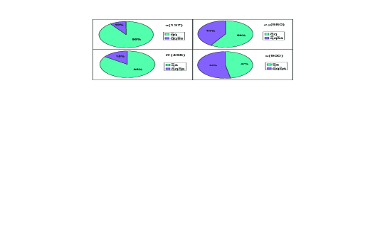
Figure 1: quark content of light isotriplets and isodoublets.

Figure 2 show the quark contents of the isoscalar-pseudoscalar mesons whereas the quark contents of isoscalar-scalar mesons is shown in figure 3.

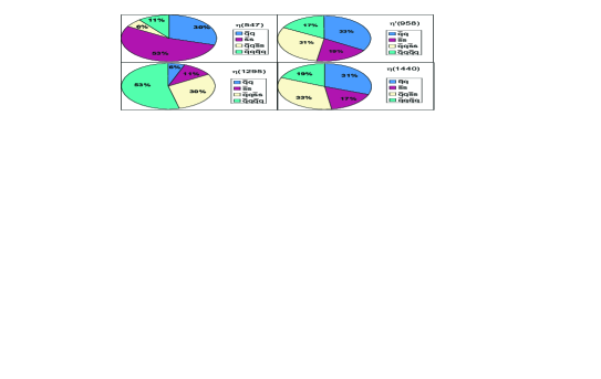
Figure 2: quark content of pseudoscalar isosinglets

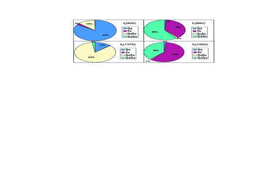
Figure 3: quark content of scalar isosinglets

It is worth to remark that the picture for isosinglets can be modified by the introduction of glueball fields which are expected to mix with isosinglet four-quark and $\overline{q}q$ states.

The light isotriplet and isodoublets, pions and kaons, arise as states mainly composed of $q\overline{q}$, whereas the heavy fields $\pi(1300),$ $K(1460)$ arise as mainly tetraquark states. In contrast, in the scalar sector isotriplets and isodoublets get strongly mixed and the physical mesons turn out to have almost identical amounts of $q\overline{q}$ and four-quark content. In the case of $\eta(547)$ we obtain also a small four-quark content, the $\eta(1295)$ being almost a four-quark state. However, the $\eta^{\prime}(958)$ and $\eta(1440),$ turn out to be strong admixtures of $q\overline{q}$ and four-quark states with almost equal amounts of them. As to the isosinglet scalars, the sigma meson ( $f_{0}(600)$) arises as mainly $q\overline{q}$ state and the opposite quark content is carried by the $f_{0}(1370)$ which turns out to be mainly a four quark state. Finally, the $f_{0}(980)$ turns out to have roughly a 40% content of $\overline{q}q$ (more explicitly $\overline{s}s$ ) and 60% of $\overline{q}\overline{q}qq$ whereas the $f_{0}(1500)$ is composed 60% of $\overline{q}q$ (more explicitly $\overline{s}s$ ) and almost 40% of $\overline{q}\overline{q}qq$. As pointed above, the quark content of isoscalar mesons as arising in this model are expected to be modified by the inclusion of glueballs in the present context, thus the picture for isoscalar mesons as arising from this analysis should be taken as very preliminary results. The need for the inclusion of glueball fields will be more transparent when we analyze interactions in the next section.

V Interactions.

As shown in the previous section, the meson spectrum is consistent with the mechanisms conjectured in this work. Another important piece of information on meson structure is the coupling to the different allowed channels. We work out the predictions of the model for the most relevant three-meson couplings and compare the predicted decay widths with experimental results for those decays where confident results exist. The different pieces in Eq. (21) relevant to the couplings we are interested are shown in Table III in terms of the parameters of the model.

Table III

Lagrangian Explicit form Couplings involved

$$\mathcal{L}_{S^{0}X^{+}X^{-}}$$

,

In order to exhibit the manipulations involved let us explicitly calculate the $g_{\sigma\pi\pi}$ coupling. The relevant piece $\mathcal{L}_{\tilde{F}\pi\pi}$ in Table III can be rewritten to

$$\mathcal{L}_{\tilde{F}\pi\pi}=-\frac{1}{\sqrt{2}a}\left[(m_{S_{ns}}^{2}-m_{P}^{2})S_{ns}+\frac{1}{2}\left(m_{F}^{2}-m_{\Sigma}^{2}\right)\sin 2\gamma S_{s}\right]P^{+}P^{-}.$$ (93)

It is possible to rewrite this Lagrangian in terms of the $\Sigma$ and $F$ fields defined as

$$S_{ns} =\cos\gamma\Sigma+\sin\gamma F,$$ (94)

$$S_{s} =-\sin\gamma\Sigma+\cos\gamma F.$$ (95)

We obtain

$$\mathcal{L}_{\tilde{F}\pi\pi}=-\frac{1}{\sqrt{2}a}\left[(m_{\Sigma}^{2}-m_{P}^{2})\cos\gamma\Sigma+(m_{F}^{2}-m_{P}^{2})\sin\gamma F\right]P^{+}P^{-}.$$ (96)

From where , upon the use of the following relations

$$m_{F}^{2} =m_{f}^{2}\cos^{2}\delta^{\prime}+m_{\hat{f}}^{2}\sin^{2}\delta^{\prime},$$ (97)

$$m_{\Sigma}^{2} =m_{\sigma}^{2}\cos^{2}\delta+m_{\hat{\sigma}}^{2}\sin^{2}\delta,$$ (98)

$$m_{p}^{2} =m_{\pi}^{2}\cos^{2}\theta_{1}+m_{\hat{\pi}}^{2}\sin^{2}\theta_{1},$$ (99)

and the expressions for $\Sigma$, $F$ and $P$ in terms of the physical fields we get

$$g_{\sigma\pi\pi}=\frac{1}{\sqrt{2}a}(m_{\sigma}^{2}+m_{\hat{\sigma}}^{2}-m_{\pi}^{2}-m_{\hat{\pi}}^{2}+\hat{\mu}_{1}^{2}-\hat{\mu}_{1/2}^{2})\cos\gamma\cos\delta\cos^{2}\theta_{1}.$$ (100)

Under similar manipulations for the appropriate pieces of the Lagrangian in Table III we obtain the couplings listed in Table IV.

Table IV

Coupling Analytic form Prediction (GeV)

$$g_{a_{0}K^{+}K^{-}}$$

Notice that in the absence of quark mass terms for tetraquarks ( $\hat{\mu}_{1}^{2}=\hat{\mu}_{1/2}^{2}$ ) and and the $\epsilon^{2}$ term, all the fields in the “nonstandard” nonet have a common mass $\hat{\mu}^{2}$ hence the couplings $g_{a_{0}K^{+}K^{-}}$, $g_{a_{0}\kappa^{+}\kappa^{-}}$ reduce to those obtained in the linear sigma model Mauro ; TornqvistEJP

$$g_{a_{0}K^{+}K^{-}}^{L\sigma M} =\frac{1}{\sqrt{2}\left(a+b\right)}\left(m_{a}^{2}-m_{K}^{2}\right),$$ (101)

$$g_{a_{0}\kappa^{+}\kappa^{-}}^{L\sigma M} =-\frac{1}{\sqrt{2}\left(b-a\right)}\left(m_{a}^{2}-m_{\kappa}^{2}\right).$$ (102)

The modifications to these couplings come from the mixing of the fields and from quark mass terms.

Unfortunately there is no much experimental information on these couplings. Recently, KLOE Collaboration kloe1 kloe2 at DA$\Phi$NE measured the di-meson mass spectrum in the rare $\varphi\longrightarrow\pi^{0}\pi^{0}\gamma$ and $\varphi\longrightarrow\pi\eta\gamma$ decays. The couplings $g_{a_{0}K^{+}K^{-}}$, $g_{f_{0}K^{+}K^{-}}$ and $g_{f_{0}\pi^{+}\pi^{-}}$ as extracted from these experiments are

$$\frac{g_{f_{0}K^{+}K^{-}}^{2}}{4\pi}|_{KLOE} =2.79\pm 0.12\text{ GeV}^{2},\qquad\frac{g_{f_{0}K^{+}K^{-}}^{2}}{g_{f_{0}\pi^{+}\pi^{-}}^{2}}|_{KLOE}=4.00\pm 0.14,$$

$$\frac{g_{a_{0}K^{+}K^{-}}^{2}}{4\pi}|_{KLOE} =0.40\pm 0.04\text{ GeV}^{2},\qquad\frac{g_{a_{0}\pi^{0}\eta}^{2}}{g_{a_{0}K^{+}K^{-}}^{2}}|_{KLOE}=1.35\pm 0.09,\qquad\frac{g_{f_{0}KK}^{2}}{g_{a_{0}KK}^{2}}|_{KLOE}=7.0\pm 0.7.$$

The predictions of the model for these quantities are

$$\frac{g_{f_{0}K^{+}K^{-}}^{2}}{4\pi}|_{\text{Model}} =0.85\pm 0.52\text{ GeV}^{2},\qquad\frac{g_{f_{0}K^{+}K^{-}}^{2}}{g_{f_{0}\pi^{+}\pi^{-}}^{2}}|_{\text{Model}}=5.16\pm 3.96,$$

$$\frac{g_{a_{0}K^{+}K^{-}}^{2}}{4\pi}|_{\text{Model}} =0.50\pm 0.23\text{ GeV}^{2},\qquad\frac{g_{a_{0}\pi^{0}\eta}^{2}}{g_{a_{0}K^{+}K^{-}}^{2}}|_{\text{Model}}=2.34\pm 1.30,\qquad\frac{g_{f_{0}KK}^{2}}{g_{a_{0}KK}^{2}}|_{\text{Model}}=1.71\pm 1.30.$$

These results give valuable information. On the one side, our $g_{a_{0}K^{+}K^{-}\text{ }}$ is in good agreement with data and the ratio $\frac{g_{a_{0}\pi^{0}\eta}^{2}}{g_{a_{0}K^{+}K^{-}}^{2}}$ is consistent with experimental results. The first quantity involves only the isodoublet and isotriplet sectors. The second one involve only the $\eta$ meson from the isoscalar sector. The prediction of the model for the isodoublet and isotriplet sectors will hardly be substantially modified by the introduction of glueball fields which are expected to impact mainly in the isoscalar sectors. In the latter sector we expect only slight modifications to the predictions for the $\eta$ meson due to its relatively low mass. On the other side, the predictions of the model for $g_{f_{0}K^{+}K^{-}}$ is smaller than KLOE measurement roughly by a factor $\sqrt{3}$. In spite of this, the ratio $\frac{g_{f_{0}K^{+}K^{-}}^{2}}{g_{f_{0}\pi^{+}\pi^{-}}^{2}}$ is in good agreement with data. A look on the analytic form of the couplings in Table IV reveals that both $g_{f_{0}K^{+}K^{-}}$ and $g_{f_{0}\pi^{+}\pi^{-}}$ depend on $\delta^{\prime}$ as $cos\delta^{\prime}.$ This factor cancels in the ratio. Furthermore this mixing angle turns out to be  unexpectedly large in the fit . We expect that upon the introduction of the lightest scalar glueball in the model this mixing angle get modified yielding more reasonable values for the couplings of the $f_{0}(980)$ meson. According to the scalar analogous to Eq. (71) the lowering of this mixing angle will also reduce the four-quark content in this meson. In this sense, the picture of isoscalar mesons as arising in this work must be considered only as a first step in the elucidation of their structure.

VI Strong decays of $a_{0}(1450)$ and $K_{0}^{\ast}(1430)$.

As discussed above, the introduction of glueball fields in the model is expected to modify its predictions for the isosinglet sectors. However, the predictions of the model for isodoublets and isotriplet sectors are not expected to be substantially modified by the introduction of glueball fields. Thus it is worthy to work out the predictions of the model for the decay widths in these sectors. Unfortunately there is no confident experimental information for pseudoscalar fields PDG , hence we will analyze the model predictions for the scalar fields where more accurate data exists. The total widths of $a_{0}(1450)$ and $K_{0}^{\ast}(1430)$ are PDG

$$\Gamma\left[a_{0}(1450)\right]_{Exp}=265\pm 13\text{ MeV,\qquad}\Gamma\left[K_{0}^{\ast}(1430)\right]_{Exp}=294\pm 23\text{ MeV,}$$ (103)

from where we obtain the fraction

$$\left.\frac{\Gamma\left[a_{0}(1450)\right]}{\Gamma\left[K^{\ast}(1430)\right]}\right|_{Exp}=0.90\pm 0.08\text{ }.$$ (104)

The measured partial widths are

$$\left.\frac{\Gamma\left[a_{0}(1450)\rightarrow\pi\eta^{\prime}\right]}{\Gamma\left[a(1450)\rightarrow\pi\eta\right]}\right|_{Exp} =0.35\pm 0.16,$$ (105)

$$\left.\frac{\Gamma\left[a_{0}(1450)\rightarrow K\overline{K}\right]}{\Gamma\left[a_{0}(1450)\rightarrow\pi\eta\right]}\right|_{Exp} =0.88\pm 0.23,$$ (106)

$$\frac{\Gamma\left[K_{0}^{\ast}(1430)\rightarrow\pi K\right]}{\Gamma\left[K_{0}^{\ast}(1430)\rightarrow\text{all}\right]} =0.93\pm 0.04\pm 0.09\text{ }.$$ (107)

From the theoretical side these decays have been studied using $SU(3)$ symmetry twononetsyr with the following predictions

$$\left.\frac{\Gamma\left[a_{0}(1450)\rightarrow\pi\eta^{\prime}\right]}{\Gamma\left[a_{0}(1450)\rightarrow\pi\eta\right]}\right|_{SU(3)} =0.16,$$ (108)

$$\left.\frac{\Gamma\left[a_{0}(1450)\rightarrow K\overline{K}\right]}{\Gamma\left[a_{0}(1450)\rightarrow\pi\eta\right]}\right|_{SU(3)} =0.55,$$ (109)

$$\left.\frac{\Gamma\left[a_{0}(1450)\right]}{\Gamma\left[K^{\ast}(1430)\right]}\right|_{SU(3)} =1.51,$$ (110)

which are in disagreement with experimental results.

In our formalism these decays are induced at the three level and are given by

$$\Gamma(S\rightarrow P_{1}P_{2})=\frac{1}{8\pi}\left|g_{SP_{1}P_{2}}\right|^{2}\frac{\left|\mathbf{p}_{1}\right|}{m_{s}^{2}}$$ (111)

where $g_{SP_{1}P_{2}}$ stands for the corresponding coupling which is extracted from Eq. (21). Using our results for the couplings in Table IV we get

$$\Gamma\left[a_{0}(1450)\rightarrow\pi\eta\right] =116.8\pm 57.6\text{ MeV,}$$ (112)

$$\Gamma\left[a_{0}(1450)\rightarrow\pi\eta^{\prime}\right] =0.00\pm 0.03\text{ MeV,}$$ (113)

$$\Gamma\left[a_{0}(1450)\rightarrow K^{+}K^{-}\right] =76.5\pm 45.6\text{ MeV,}$$ (114)

$$\Gamma\left[K^{\ast}(1430)\rightarrow\pi K\right]=396.6\pm 262.4\text{ MeV.}$$ (115)

The decay width $\Gamma\left[a(1450)\rightarrow K\bar{K}\right]$ = $2\Gamma[a(1450)\rightarrow$ $K^{+}K^{-}]$ and assuming those three decay modes are the dominant ones we get

$$\Gamma\left[a_{0}(1450)\right]=269.9\pm 107.9\text{ MeV.}$$ (116)

This yields

$$\frac{\Gamma(a(1450)\rightarrow K\bar{K})}{\Gamma(a(1450)\rightarrow\pi\eta)}=1.31\pm 1.01$$

consistent with the value quoted in Eq. (106) for this fraction. Notice however that the fraction of the $\pi\eta^{\prime}$ to $\pi\eta$ partial widths turns out to be small in the model as compared with experiment a result due to the prediction of a decay width consistent with zero for $\pi\eta^{\prime}$ channel. Again, the $\eta^{\prime}$ is expected to contain certain amount of glueball which is not included in the present context. For the fraction in Eq. (104) the model yields

$$\frac{\Gamma\left[a(1450)\right]}{\Gamma\left[K^{\ast}(1430)\right]}=0.68\pm 0.53$$ (117)

consistent with experimental results.

VII Summary and perspectives.

Summarizing, in this paper we point out the existence of a quasi-degenerate chiral nonet around 1.4 GeV whose scalar part presents a slightly inverted spectrum as compared with expectations from a conventional $\overline{q}q$ nonet. Guided by the empirical linear rising of the mass of a hadron with the number of constituent quarks and the fact that a four-quark nonet should present an inverted spectrum as pointed out long ago by Jaffe Jaffe:1977 , we conjecture that this cuasi-degenerate chiral nonet and the lowest lying scalar and pseudoscalar mesons, come from the mixing of a chiral $\overline{q}\overline{q}qq$ nonet (chiral symmetry realized directly) with a conventional $\overline{q}q$ chiral nonet (chiral symmetry spontaneously broken). We realize these ideas in the framework of an effective chiral model. We introduce quark mass terms appropriate to four-quark states which give to these states an inverted spectrum. Particularly important for the $\overline{q}q$ states is the instanton induced effective trilinear interaction. We fix the parameters of the model using as input the masses for $\pi(137)$, $a_{0}(980)$, $K(495),$ $\eta(548),$ $\eta^{\prime}(957),$ $\eta(1295)$ in addition to the weak decay constants $f_{\pi}$ and $f_{K}$. The model gives definite predictions for the masses of the remaining members of the nonets and the couplings of all mesons entering the model. The outcome of the fit allow us to identify the remaining mesons as the $\pi(1300),$ $\eta(1450),$ $K(1469)$ on the pseudoscalar side and $f_{0}(1370),$ $K_{0}^{\ast}(1430),$ $a_{0}(1450),$ $f_{0}(1500)$ on the scalar side. In general, isospinor and isovector pseudoscalar mesons arise as weak mixing of $\overline{q}q$ and tetraquark fields. In contrast, scalars in these isotopic sectors get strongly mixed. We obtain also strong mixing between $\overline{q}q$ and tetraquarks for isoscalar fields. We work out the model predictions for the most relevant couplings and calculate explicitly the strong decays of the $a_{0}(1450)$ and $K_{0}^{\ast}(1430)$ mesons. From the comparison of the predicted couplings with the experimental ones we conclude that observable for the isovector and isospinor sectors are consistently described within the model. However, although the masses in the isoscalar sectors are consistent with the conjecture mentioned above, the couplings are not all properly described. However, the states entering the model lie at an energy quite close to the expected mass for the lightest glueballs. We expect the inclusion of these states to provide the missing ingredients to reach a consistent global picture of pseudoscalar and scalar mesons below $1.5$ $GeV$. The introduction of these fields in the present context can be easily done since these states behave as singlets with respect to chiral transformations. Furthermore these fields can acquire non-vanishing vacuum expectation values rendering the glueball-meson-meson interactions natural candidates to generate the (somewhat artificial) mixing term (or similar ones) in Eq. (15) in a simple and straightforward way. On the experimental side, there is a unique candidate in the scalar sector for the missing state, the $f_{0}(1710)$, once we introduce the lightest scalar glueball. All states above 1 GeV, including the $f_{0}(1710)$, are expected to acquire a glueball component to some extent.

Another piece of information which could prove relevant is a direct mixing between $\ \overline{q}q$ and $\overline{q}\overline{q}qq$ states due to instantons which is not included here. These possibilities are presently under investigation. Predictions of the model for the two photon decay of neutral scalars will be published elsewhere twophotons .

References

• (1) N. N. Achasov, S. A. Devyanin and G. N. Shestakov, Phys. Lett. B 88, 367 (1979); N. N. Achasov and G. N. Shestakov, Phys. Rev. D 56, 212 (1997) [arXiv:hep-ph/9610409]; N. N. Achasov and A. V. Kiselev, Phys. Lett. B 534, 83 (2002) [arXiv:hep-ph/0203042].
• (2) F. E. Close and A. Kirk, Phys. Lett. B 489, 24 (2000) [arXiv:hep-ph/0008066]; Phys. Lett. B 515, 13 (2001) [arXiv:hep-ph/0106108]; O. Krehl, R. Rapp and J. Speth, Phys. Lett. B 390, 23 (1997) [arXiv:nucl-th/9609013].
• (3) A. Gallegos and J. L. Lucio M., Found. Phys. 33, 855 (2003).
• (4) N. A. Tornqvist, Phys. Rev. Lett. 49, 624 (1982); Z. Phys. C 68, 647 (1995) [arXiv:hep-ph/9504372]; N. A. Tornqvist and M. Roos, Phys. Rev. Lett. 76, 1575 (1996) [arXiv:hep-ph/9511210].
• (5) E. Van Beveren, T. A. Rijken, K. Metzger, C. Dullemond, G. Rupp and J. E. Ribeiro, Z. Phys. C 30, 615 (1986).
• (6) M. D. Scadron, Phys. Rev. D 26, 239 (1982).
• (7) M. Harada, F. Sannino and J. Schechter, Phys. Rev. D 54, 1991 (1996) [arXiv:hep-ph/9511335].
• (8) S. Ishida, M. Ishida, H. Takahashi, T. Ishida, K. Takamatsu and T. Tsuru, Prog. Theor. Phys. 95, 745 (1996) [arXiv:hep-ph/9610325].
• (9) M. Napsuciale, arXiv:hep-ph/9803396, unpublished.
• (10) N. A. Tornqvist, Eur. Phys. J. C 11, 359 (1999) [arXiv:hep-ph/9905282].
• (11) C. Caso et al. [Particle Data Group Collaboration], Eur. Phys. J. C 3, 1 (1998).
• (12) J. A. Oller, E. Oset and J. R. Pelaez, Phys. Rev. Lett. 80, 3452 (1998) [arXiv:hep-ph/9803242]; Phys. Rev. D 59 , 074001 (1999) [Erratum-ibid. D 60, 099906 (1999)] [arXiv:hep-ph/9804209]; J. A. Oller and E. Oset, Phys. Rev. D 60, 074023 (1999) [arXiv:hep-ph/9809337].
• (13) E. M. Aitala et al. [E791 Collaboration], Phys. Rev. Lett. 86, 770 (2001) [arXiv:hep-ex/0007028]; Phys. Rev. Lett. 86, 765 (2001) [arXiv:hep-ex/0007027].
• (14) S. Ishida, M. Ishida, T. Ishida, K. Takamatsu and T. Tsuru, Prog. Theor. Phys. 98, 621 (1997) [arXiv:hep-ph/9705437].
• (15) D. Black, A. H. Fariborz, F. Sannino and J. Schechter, Phys. Rev. D 58, 054012 (1998) [arXiv:hep-ph/9804273].
• (16) E. M. Aitala et al. [E791 Collaboration], Phys. Rev. Lett. 89, 121801 (2002) [arXiv:hep-ex/0204018].
• (17) S. N. Cherry and M. R. Pennington, Nucl. Phys. A 688, 823 (2001) [arXiv:hep-ph/0005208].
• (18) D. Black, A. H. Fariborz, F. Sannino and J. Schechter, Phys. Rev. D 59, 074026 (1999) [arXiv:hep-ph/9808415].
• (19) J. A. Oller, Nucl. Phys. A 727, 353 (2003) [arXiv:hep-ph/0306031].
• (20) T. Barnes, Phys. Lett. B 165, 434 (1985).
• (21) M. Napsuciale, AIP Conf. Proc. 623, 131 (2002) [arXiv:hep-ph/0204170].
• (22) R. Jaffe, Phys. Rev. D15 (1977) 267.
• (23) J. Weinstein and N. Isgur, Phys. Rev. D41 (1990) 2236.
• (24) M. G. Alford and R. L. Jaffe, Nucl. Phys. B 578, 367 (2000) [arXiv:hep-lat/0001023].
• (25) R. R. Akhmetshin et al. [CMD-2 Collaboration], Phys. Lett. B 462, 380 (1999) [arXiv:hep-ex/9907006]; Phys. Lett. B 462, 371 (1999) [arXiv:hep-ex/9907005].
• (26) A. Aloisio et al. [KLOE Collaboration], Phys. Lett. B 537, 21 (2002) [arXiv:hep-ex/0204013]; Phys. Lett. B 536, 209 (2002) [arXiv:hep-ex/0204012].
• (27) M. Napsuciale and S. Rodriguez, Int. J. Mod. Phys. A 16, 3011 (2001) [arXiv:hep-ph/0204149].
• (28) M. Napsuciale, A. Wirzba and M. Kirchbach, Nucl. Phys. A 703, 306 (2002) [arXiv:nucl-th/0105055].
• (29) J. Schechter and Y. Ueda, Phys. Rev. D3, 2874 (1971).
• (30) G. ’t Hooft, Phys. Rev. D 14, 3432 (1976) [Erratum-ibid. D 18, 2199 (1978)]; arXiv:hep-th/9903189, unpublished;
• (31) J. L. Lucio Martinez and M. Napsuciale, Phys. Lett. B 454, 365 (1999) [arXiv:hep-ph/9903234].
• (32) A. Bramon, R. Escribano, J. L. Lucio M., M. Napsuciale and G. Pancheri, Phys. Lett. B 494, 221 (2000) [arXiv:hep-ph/0008188]; Eur. Phys. J. C 26, 253 (2002) [arXiv:hep-ph/0204339]. A. Bramon, R. Escribano, J. L. Lucio Martinez and M. Napsuciale, Phys. Lett. B 517, 345 (2001) [arXiv:hep-ph/0105179].
• (33) M. Napsuciale and S. Rodriguez, Phys. Rev. D65, 096013 (2002) [arXiv:hep-ph/0112105].
• (34) D. Black, A. H. Fariborz and J. Schechter, Phys. Rev. D61, 074001 (2000) [arXiv:hep-ph/9907516].
• (35) D. Black, A. H. Fariborz, S. Moussa, S. Nasri and J. Schechter, Phys. Rev. D64, 014031 (2001) [arXiv:hep-ph/0012278].
• (36) N. A. Tornqvist, arXiv:hep-ph/0201171; F. E. Close and N. A. Tornqvist, J. Phys. G28, R249 (2002) [arXiv:hep-ph/0204205].
• (37) K. Hagiwara et al. [Particle Data Group Collaboration], Phys. Rev. D66, 010001 (2002).
• (38) M. Svec, A. de Lesquen, L.van Rossum Phys. Rev. D45 (1992) 1518.
• (39) A. Aloisio et al. [KLOE Collaboration], Phys. Lett. B 536, 209 (2002) [arXiv:hep-ex/0204012].
• (40) A. Aloisio et al. [KLOE Collaboration], Phys. Lett. B 537, 21 (2002) [arXiv:hep-ex/0204013].
• (41) ”Two photon decay of neutral scalars in a chiral model for $\overline{q}q$ and $\overline{q}\overline{q}qq$ mesons”, M. Napsuciale, S. Rodríguez, in preparation.