Abstract

Classic statistical techniques (like the multi-dimensional likelihood and the Fisher discriminant method) together with Multi-layer Perceptron and Learning Vector Quantization Neural Networks have been systematically used in order to find the best sensitivity when searching for $\nu_{\mu}\to\nu_{\tau}$ oscillations. We discovered that for a general direct $\nu_{\tau}$ appearance search based on kinematic criteria: a) An optimal discrimination power is obtained using only three variables ($E_{visible}$, $P_{T}^{miss}$ and $\rho_{l}$) and their correlations. Increasing the number of variables (or combinations of variables) only increases the complexity of the problem, but does not result in a sensible change of the expected sensitivity. b) The multi-layer perceptron approach offers the best performance. As an example to assert numerically those points, we have considered the problem of $\nu_{\tau}$ appearance at the CNGS beam using a Liquid Argon TPC detector.

1 Introduction

The experimental confirmation that atmospheric and solar neutrinos do oscillate [1, 2], and therefore have mass, represents the first solid clue for the existence of new physics beyond the Standard Model [3]. Results from experiments carried out with neutrinos produced in artificial sources, like reactors and accelerators, strongly support the fact that neutrinos are massive [4, 5].

Notwithstanding the impressive results achieved by current experiments, neutrino phenomenology is a very rich and active field, where plenty of open questions still await for a definitive answer. Thus, many next-generation neutrino experiments are being designed and proposed to measure with precision the parameters that govern the oscillation (mass differences and mixing angles) [6]. New facilities like super-beams, beta beams [7] and neutrino factories [8] have been put forward and their performances studied in detail in order to ascertain whether they can give an answer to two fundamental questions: what is the value of the mixing angle between the first and the third family, and whether CP violation takes place in the leptonic sector [9].

Recently, the Super-Kamiokande Collaboration has measured a first evidence of the sinusoidal behaviour of neutrino disappearance as dictated by neutrino oscillations [10]. However, although the most favoured hypothesis for the observed $\nu_{\mu}$ disappearance is that of $\nu_{\mu}\to\nu_{\tau}$ oscillations, no direct evidence for $\nu_{\tau}$ appearance exists up to date. A long baseline neutrino beam, optimized for the parameters favoured by atmospheric oscillations, has been approved in Europe to look for explicit $\nu_{\tau}$ appearance: the CERN-Laboratori Nazionali del Gran Sasso (CNGS) beam [11]. The approved experimental program consists of two experiments ICARUS [12] and OPERA [13] that will search for $\nu_{\mu}\to\nu_{\tau}$ oscillations using complementary techniques.

Given the previous experimental efforts [14, 15] and present interest in direct $\nu_{\tau}$ appearance, we assess in this note the performance of several statistical techniques applied to the search for $\nu_{\tau}$ using kinematic techniques. Classic statistical methods (like multi-dimensional likelihood and Fischer’s discriminant schemes) and Neural Networks based ones (like multi-layer perceptron and self-organized neural networks) have been applied in order to find the approach that offers the best sensitivity.

2 Oscillation Search Using Kinematic Criteria

The original proposal to observe for the first time the direct appearance of a $\nu_{\tau}$ by means of kinematic criteria dates back to 1978 [16]. Based on the capabilities to measure the direction of the hadronic jet, the interaction of the neutrino associated with the tau lepton can be spotted thanks to: a) the presence of a sizable missing transverse momentum; b) certain angular correlations between the direction of the prompt lepton and the hadronic jet, in the plane transverse to the incoming neutrino beam direction.

NOMAD [14] was a pioneering experiment in the use of kinematic criteria applied to a $\nu_{\mu}\to\nu_{\tau}$ oscillation search. The kinematic approach was validated after several years of successful operation at the CERN WANF neutrino beam [17, 18]. This short-baseline experiment set the most competitive limit for $\nu_{\mu}\to\nu_{\tau}$ oscillations at high values of $\Delta m^{2}$ [19].

An impressive background rejection power O($10^{5}$) was needed in NOMAD. To achieve this, a multidimensional likelihood was built taking advantage of: on the one hand, the different event kinematics for signal and background events; on the other, the existing correlations among the variables used. To further enhance the sensitivity, the signal region was divided into several bins.

Given the interest that $\nu_{\mu}\to\nu_{\tau}$ oscillation searches have nowadays for the region of $\Delta m^{2}\sim 10^{-3}$ eV², we have considered the problem of finding the statistical approach that offers the best sensitivity for this kind of search. Unlike NOMAD, we do not try to improve the sensitivity by splitting the signal regions into a set of independent bins.

We have simply compared the discrimination power offered by a multi-dimensional likelihood, the Fisher discriminant method and a neural network. As a general conclusion, we have observed that neural networks offer the best background rejection power thanks to their ability to find complex correlations among the kinematic variables. In addition, they allow to reduce the complexity of the problem, given that a small number of input variables is enough to optimize the experimental sensitivity. These conclusions are valid for direct $\nu_{\tau}$ appearance searches performed either with atmospheric or accelerator neutrinos. In what follows we give a numerical example that illustrates the conclusions of this study.

3 Detector Configuration and Data Simulation

To obtain a numerical evaluation of the performances of the different statistical techniques we used, and assess which of them gives the best sensitivity when searching for direct $\nu_{\tau}$ appearance by means of kinematic criteria, we have considered the particular case of the CNGS beam.

We assume a detector configuration consisting of 3 ktons of Liquid Argon [12]. In our simulation the total mass of active (imaging) Argon amounts to 2.35 ktons. We assumed five years running of the CNGS beam in shared mode ($4.5\times 10^{19}$ p.o.t. per year), which translates into a total exposure of $5\times 2.35=11.75$ kton$\times$year. The total event rates expected are 252 (17) $\nu_{e}\ (\bar{\nu}_{e})$ CC events and 50 $\nu_{\tau}$ CC events with the $\tau$ decaying into an electron plus two neutrinos (we assume maximal mixing and $\Delta m_{23}^{2}=3\times 10^{-3}$ eV²; these values are compatible with the allowed range given by atmospheric neutrinos). Before cuts, the signal over background ratio, in active LAr, is $50/252\simeq 0.2$.

The study of the capabilities to reconstruct and analyze high-energy neutrino events was done using fully simulated $\nu_{e}$CC events inside the whole LAr active volume. Neutrino cross sections and the generation of neutrino interactions is based on the NUX code [20]; final state particles are then tracked using the FLUKA package [21]. The angular and energy resolutions used in the simulation of final state electrons and individual hadrons are identical to those quoted in [12].

In order to apply the most efficient kinematic selection, it is mandatory to reconstruct with the best possible resolution the energy and the angle of the hadronic jet and the prompt lepton, with particular attention to the tails of the distributions. Therefore, the energy flow algorithm has been designed with care, taking into account the needs of the tau search analysis.

The ability to look for tau appearance events is limited by the containment of high energy neutrino events. Energy leakage outside the active imaging volume creates tails in the kinematic variables that fake the presence of neutrinos in the final state. We therefore impose fiducial cuts in order to guarantee that on average the events will be sufficiently contained.

The fiducial volume is defined by looking at the profiles of the total missing transverse momentum and of the total visible energy of the events. The average value of these variables is a good estimator of how much energy is leaking on average. After fiducial cuts, we keep 65% of the total number of events occurring in the active LAr volume. This means a total exposure of 7.6 kton$\times$year after five years of shared CNGS running.

Table 1 summarizes the total amount of simulated data used for this study. We note that $\nu_{\tau}\ (\nu_{e})$ CC sample, generated in active LAr, is more than a factor 250 (50) larger than the expected number of collected events after five years of CNGS running.

Process	$\nu_{e}$CC	$\nu_{\tau}$CC
		($\tau\rightarrow e$)
Active LAr	14200 [252]	13900 [50]
Fiducial Vol.	9250[163]	9000[33]

Table 1: Amount of fully generated data in Active and Fiducial LAr volumes. Between brackets we show the expected number of events after five years of data taking at CNGS with a 3 kton detector.

4 Statistical Pattern Recognition Applied to Oscillation Searches

In the case of a $\nu_{\mu}\rightarrow\nu_{\tau}$ oscillation search with Liquid Argon, the golden channel to look for $\nu_{\tau}$ appearance is the decay of the tau into an electron and a pair neutrino anti-neutrino due to: (a) the excellent electron identification capabilities; (b) the low background level, since the intrinsic $\nu_{e}$ and $\bar{\nu}_{e}$ charged current contamination of the beam is at the level of one per cent.

Kinematic identification of the $\tau$ decay [18], which follows the $\nu_{\tau}$CC interaction, requires excellent detector performance: good calorimetric features together with tracking and topology reconstruction capabilities. In order to separate $\nu_{\tau}$ events from the background, a basic criteria can be used: an unbalanced total transverse momentum due to neutrinos produced in the $\tau$ decay.

In figure 1 we illustrate the difference on kinematics for signal and background events. We plot four of the most discriminating variables:

• $E_{vis}$: Visible energy.

• $P_{T}^{miss}$: Missing momentum in the transverse plane with respect to the direction of the incident neutrino beam.

• $P_{T}^{lep}$: Transverse momentum of the prompt electron candidate.

• $\rho_{l}=\frac{{\textstyle P_{T}^{lep}}}{{\textstyle P_{T}^{lep}+P_{T}^{had}+P_{T}^{miss}}}$

Signal events tend to accumulate in low $E_{vis}$, low $P_{T}^{lep}$, low $\rho_{l}$ and high $P_{T}^{miss}$ regions.

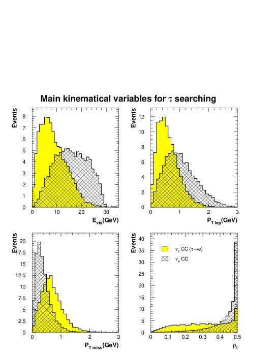
Figure 1: Visible energy (top left), transverse missed momentum (bottom left), transverse electron momentum (top right) and $\rho_{l}$ (bottom right). Histograms have an arbitrary normalization.

Throughout this article, we take into account only the background due to electron neutrino charged current interactions. Due to the low content the beam has on $\bar{\nu}_{e}$, charged currents interactions of this type have been observed to give a negligible contribution to the total expected background. We are confident that neutral current background can be reduced to a negligible level using LAr imaging capabilities and algorithms based on the different energy deposition showed by electrons and $\pi^{0}$(see for example [22]). Therefore it will not be further considered. The contamination due to charm production and $\nu_{\mu}$ CC events, where the prompt muon is not identified as such, was studied by the ICARUS Collaboration [23] and showed to be less important than $\nu_{e}$CC background.

4.1 Oscillation Search Using Classic Statistical Methods

4.1.1 The Multi-dimensional Likelihood

The first method adopted for the $\tau$ appearance search is the construction of a multi-dimensional likelihood function (see for example [24]), which is used as the unique discriminant between signal and background. This approach is, a priori, an optimal discrimination tool since it takes into account correlations between the chosen variables.

A complete likelihood function should contain five variables (three providing information of the plane normal to the incident neutrino direction and two more providing longitudinal information). However, in a first approximation, we limit ourselves to the discrimination information provided by the three following variables: $E_{visible}$, $P_{T}^{miss}$ and $\rho_{l}$.

As we will see later, all the discrimination power is contained in these variables, therefore we can largely reduce the complexity of the problem without affecting the sensitivity of the search. Two likelihood functions were built, one for $\tau$ signal ($\mathcal{L_{S}}$) and another for background events ($\mathcal{L_{B}}$). The discrimination was obtained by taking the ratio of the two likelihoods:

$$ln(\lambda)\equiv\mathcal{L}([E_{visible},P_{T}^{miss},\rho_{l}])=\frac{\mathcal{L_{S}}([E_{visible},P_{T}^{miss},\rho_{l}])}{\mathcal{L_{B}}([E_{visible},P_{T}^{miss},\rho_{l}])}$$ (1)

In order to avoid a bias in our estimation, half of the generated data was used to build the likelihood functions and the other half was used to evaluate overall efficiencies. Full details about the multi-dimensional likelihood algorithm can be found elsewhere [22]. However, we want to point out here some important features of the method.

A partition of the hyperspace of input variables is required: The multi-dimensional likelihood will be, in principle, defined over a lattice of bins. The number of bins to be filled when constructing likelihood tables grows like $n^{d}$ where $n$ is the number of bins per variable and $d$ the number of these variables. This leads to a “dimensionality” problem when we increment the number of variables, since the amount of data required to have a well defined value for ln$\lambda$ in each bin of the lattice will grow exponentially.

In order to avoid regions populated with very few events, input variables must be redefined to have the signal uniformly distributed in the whole input hyperspace, hence $E_{visible}$, $P_{T}^{miss}$ and $\rho_{l}$ are replaced by “flat” variables (see figure 2). Besides, an adequate smoothing algorithm is needed in order to alleviate fluctuations in the distributions in the hyperspace and also, to provide a continuous map from the input variables to the multi-dimensional likelihood one (ln$\lambda$).

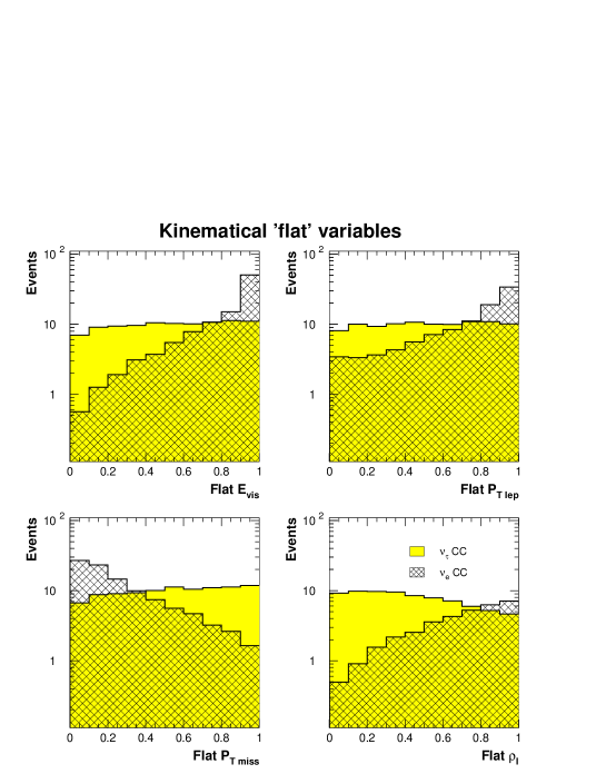
Figure 2: Comparison for “flat” $E_{visible}$, $P_{T}^{lep}$, $\rho_{l}$ and $P_{T}^{miss}$ variables between $\tau$ signal and $\nu_{e}$ CC events. Arbitrary normalization has been taken into account when plotting background events.

Ten bins per variable were used, giving rise to a total of $10^{3}$ bins. Figure 3 shows the likelihood distributions for background and tau events assuming five years running of CNGS (total exposure of 7.6 kton $\times$ year for events occurring inside the fiducial volume).

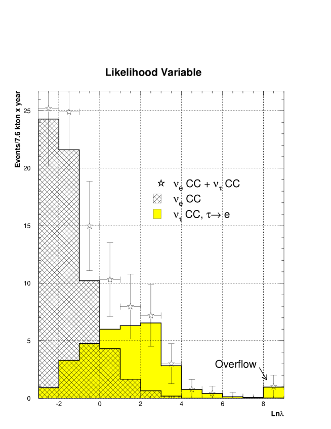
Figure 3: Multi-dimensional likelihood distributions for $\nu_{e}$ CC and $\tau\rightarrow e$ events. The last bin in signal includes the event overflow. Error bars in $\nu_{e}$CC + $\nu_{\tau}$CC sample represent statistical fluctuations in the expected profile measurements after 5 years of data taking with shared running CNGS and a 3 kton detector configuration.

Table 2 shows, for different cuts of $\ln\lambda$, the expected number of tau and $\nu_{e}$ CC background events. As reference for future comparisons, we focus our attention in the cut ln$\lambda>1.8$. It gives a signal selection efficiency around 25% (normalized to the total number of $\tau$ events in active LAr). This $\tau$ efficiency corresponds to 12.9 signal events. For this cut, we expect $1.1\pm 0.2$ background events. After cuts are imposed, this approach predicts a S/B ratio similar to 13.

	$\nu_{\tau}$CC $(\tau\rightarrow e)$		$\nu_{\tau}$ CC $(\tau\rightarrow e)$
Cuts	Efficiency	$\nu_{e}$CC	$\Delta m^{2}=$
	($\%$)		$3\times 10^{-3}$ eV2
Initial	100	252	50
Fiducial volume	65	163	33
$\ln\lambda>0.0$	48	$6.8\pm 0.5$	$24.0\pm 0.6$
$\ln\lambda>0.5$	42	$3.6\pm 0.3$	$20.8\pm 0.6$
$\ln\lambda>1.0$	36	$2.5\pm 0.3$	$18.0\pm 0.6$
$\ln\lambda>1.5$	30	$1.7\pm 0.2$	$15.2\pm 0.5$
ln $\mathbf{\lambda>1.8}$	25	$\mathbf{1.1\pm 0.2}$	$\mathbf{12.9\pm 0.5}$
ln $\lambda>2.0$	23	$0.86\pm 0.16$	$11.7\pm 0.5$
$\ln\lambda>2.5$	16	$0.40\pm 0.12$	$8.1\pm 0.4$
$\ln\lambda>3.0$	10	$0.22\pm 0.08$	$5.2\pm 0.3$
$\ln\lambda>3.5$	7	$0.12\pm 0.06$	$3.3\pm 0.2$

Table 2: Expected number of $\nu_{e}$CC background and signal events in the $\tau\rightarrow e$ analysis. A multi-dimensional likelihood function is used as the unique discriminant. Numbers are normalized to 5 years running of CNGS. Errors in the number of expected events are of statistical nature.

4.1.2 The Fisher Discriminant Method

The Fisher discriminant method [24] is a standard statistical procedure that, starting from a large number of input variables, allows us to obtain a single variable that will efficiently distinguish among different hypotheses. As in the likelihood method, the Fisher discriminant will contain all the discrimination information.

The Fisher approach tries to find a linear combination of the following kind

$$t(\{x_{j}\})=a_{0}+\sum_{i=1}^{n}a_{i}x_{i}$$

of an initial set of variables $\{x_{j}\}$ which maximizes

$$J(\{a_{j}\})=\frac{(\bar{t}_{sig}-\bar{t}_{bkg})^{2}}{(\sigma_{sig}^{2}-\sigma_{bkg}^{2})}$$ (2)

where $\bar{t}$ is the mean of the $t$ variable and $\sigma$ its variance. This last expression is nothing but a measure, for the variable $t$, of how well separated signal and background are. Thus, by maximizing (2) we find the optimal linear combination of initial variables that best discriminates signal from background. The parameters $a_{j}$ which maximize (2) can be obtained analytically by (see [24])

$$a_{i}=W_{ij}^{-1}(\mu_{j}^{sig}-\mu_{j}^{bkg})$$ (3)

where $\mu_{j}^{sig}$ and $\mu_{j}^{bkg}$ are the mean in the variable $x_{j}$ for signal and background respectively, and $W=V_{sig}+V_{bkg}$, being $V$ the covariance matrices.

A Fisher Function for $\nu_{\tau}$ Appearance Search

From the distributions of kinematic variables for $\nu_{\tau}$CC and $\nu_{e}$CC, we can immediately construct a Fisher function for a given set of variables. Initially we select the same set of variables we used for the likelihood approach, namely: $E_{visible}$, $P_{T}^{miss}$ and $\rho_{l}$. We need only the vector of means and covariance matrices in order to calculate the optimum Fisher variable (equation 3). Distributions are shown in figure 4, where the usual normalization has been assumed. In table 3 values for the expected number of signal and background events are shown as a function of the cut on the Fisher discriminant. Since linear correlations among variables are taken into account, the Fisher discriminant method offers similar results to the one obtained using a multi-dimensional likelihood.

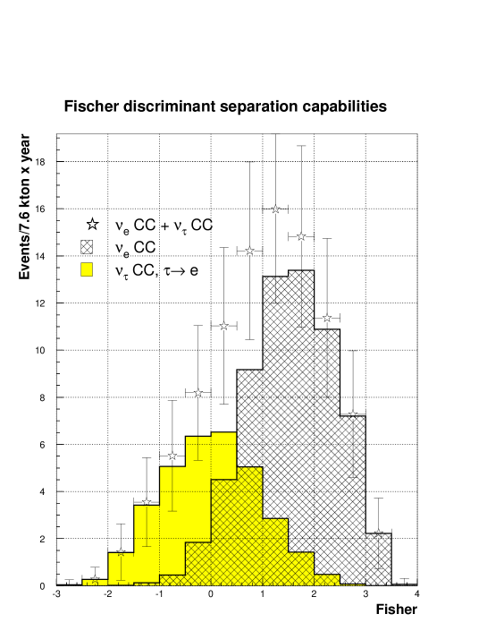
Figure 4: The Fischer discriminant variable. Error bars in $\nu_{e}$CC + $\nu_{\tau}$CC sample represent statistical fluctuations in the expected profile measurements after 5 years of data taking with shared running CNGS and a 3 kton detector configuration

	$\nu_{\tau}$CC ($\tau\rightarrow e$)		$\nu_{\tau}$ CC ($\tau\rightarrow e$)
Cuts	Efficiency	$\nu_{e}$CC	$\Delta m^{2}=$
	(%)		$3\times 10^{-3}$ eV2
Initial	100	252	50
Fiducial volume	65	164	33
Fisher$>0.5$	46	$6.9\pm 0.3$	$23.1\pm 0.4$
Fisher$>0.0$	33	$2.4\pm 0.2$	$16.6\pm 0.4$
Fisher$\mathbf{>-0.27}$	25	$\mathbf{1.15\pm 0.13}$	$\mathbf{12.9\pm 0.3}$
Fisher$>-0.5$	20	$0.60\pm 0.10$	$10.2\pm 0.3$
Fisher$>-1.0$	10	$0.14\pm 0.05$	$5.2\pm 0.2$

Table 3: Expected number of $\nu_{e}$CC background and signal events in the $\tau\rightarrow e$ analysis. A Fisher variable is used as the unique discriminant. Numbers are normalized to 5 years running of CNGS. Errors in the number of expected events are of statistical nature.

Contrary to what happens with a multi-dimensional likelihood (where the increase in the number of discriminating variables demands more Monte-Carlo data and therefore it is an extreme CPU-consuming process), the application of the Fisher method to a larger number of kinematic variables is straightforward, since the main characteristic of the Fisher method is that the final discriminant can be obtained algebraically from the initial distributions of kinematic variables. For instance, a Fisher discriminant built out of 9 kinematic variables ($E_{vis}$, $P_{T}^{miss}$, $\rho_{l}$, $P_{T}^{lep}$, $E_{lep}$, $\rho_{m}$, $Q_{T}$, $m_{T}$, $Q_{lep}$) predicts for $12.9\pm 0.3$ taus a background of $1.17\pm 0.14$ $\nu_{e}$ CC events. We conclude that, for the Fisher method, increasing the number of variables does not improve the discrimination power we got with the set $E_{vis}$, $P_{T}^{miss}$, $\rho_{l}$ and therefore these three variables are enough to perform an efficient $\tau$ appearance search.

4.2 Oscillation Search Using Neural Networks

In the context of signal vs background discrimination, neural networks arise as one of the most powerful tools. The crucial point that makes these algorithms so good is their ability to adapt themselves to the data by means of non-linear functions.

Artificial Neural Networks have become a promising approach to many computational applications. It is a mature and well founded computational technique able to learn the natural behaviour of a given data set, in order to give future predictions or take decisions about the system that data represent (see [25] and [26] for a complete introduction to neural networks). During last decade, neural networks have been widely used to solve High Energy Physics problems (see [27] for a introduction to neural networks techniques and applications to HEP). Multi-layer perceptrons efficiently recognize signal features from an, a priori, dominant background environment ([28], [29]).

We have evaluated the performance offered by neural networks when looking for $\nu_{\mu}\rightarrow\nu_{\tau}$ oscillations. As in the case of a multi-dimensional likelihood, a single valued function will be the unique discriminant. This is obtained adjusting the free parameters of our neural network model by means of a training period. During this process, the neural network is taught to distinguish signal from background using a learning data sample.

Two different neural networks models have been studied: the multi-layer perceptron and the learning vector quantization self-organized network. In the following, the results obtained with both methods are discussed.

4.2.1 The Multi-layer Perceptron

The multi-layer perceptron (MLP) function has a topology based on different layers of neurons which connect input variables (the variables that define the problem, also called feature variables) with the output unit (see figure 5). The value (or ”state”) a neuron has, is a non-linear function of a weighted sum over the values of all neurons in the previous layer plus a constant, called bias:

$$s_{i}^{l}=g\,(\sum_{j}\omega_{ij}^{l}s_{j}^{l-1}+b_{i}^{l})$$ (4)

where $s_{i}^{l}$ is the value of the neuron $i$ in layer $l$; $\omega_{ij}^{l}$ is the weight associated to the link between neuron $i$ in layer $l$ and neuron $j$ in the previous layer $(l-1)$; $b_{i}^{l}$ is a bias defined in each neuron and $g(x)$ is called the transfer function. The transfer function is used to regularize the neuron’s output to a bounded value between 0 and 1 (or -1,1).

Figure 5: A general multi-Layer perceptron diagram. The optimal non-linear function of input variables ($x_{i}$) is constructed using a set of basic units called neurons. Each neuron has two free parameters that must be adjusted minimizing an error function.

In a multi-layer perceptron, a non-linear function is used to obtain the discriminating variable. Therefore complex correlations among variables are taken into account, thus enhancing background rejection capabilities.

The construction of a MLP implies that several choices must be made a priori: amount of input variables, hidden layers, neurons per layer, number of epochs, etc. The size of the simulated data set is also crucial in order to optimize the training algorithm performance. If the training sample is small, it is likely for the MLP to adjust itself extremely well to this particular data set, thus losing generalization power (when this occurs the MLP is over-learning the data).

Multi-layer Perceptron for $\nu_{\tau}$ Appearance Search

As already mentioned in 4.1.1, we fully define our tagging problem using five variables (three in the transverse plane and two in longitudinal direction), since they utterly describe the event kinematics, provided that we ignore the jet structure. Initially we build a MLP that contains only three input variables, and in a latter step we incorporate more variables to see how the discrimination power is affected. The three chosen variables are $E_{visible}$, $P_{T}^{miss}$ and $\rho_{l}$. Our election is similar to the one used for the multi-dimensional likelihood approach. This allows us to make a direct comparison of the sensitivities provided by the two methods.

Figure 6: Chosen topology for the MLP. We feed a two layered MLP (4 neurons in first layer and 1 in second) with input variables: $E_{visible}$, $P_{T}^{miss}$ and $\rho_{l}$.

The implementation of the multilayer perceptron was done by means of the MLPfit package [30], interfaced in PAW. Among the set of different neural network topologies that we studied, we saw that the optimal one is made of two hidden layers with four neurons in the first hidden layer and one in the second (see figure 6).

Simulated data was divided in three, statistically independent, subsets of 5000 events each (consisting of 2500 signal events and an identical amount of background).

The MLP was trained with a first “learning” data sample. Likewise, the second “test” data set was used as a training sample to check that over-learning does not occur. Once the MLP is set, the evaluation of final efficiencies is done using the third independent data sample (namely, a factor 40 (75) larger than what is expected for background (signal) after five years of CNGS running with a 3 kton detector).

Error curves during learning are shown in figure 7 for training and test samples. We see that even after 450 epochs, over-learning does not take place. Final distributions in the multi-layer perceptron discriminating variable can be seen in figure 8.

Figure 7: Learning curves for the MLP. The neural network is trained for 450 epochs in order to reach a stable minimum. The solid line represents the error on training sample, the dashed line is the error on the test sample. Both lines run almost parallel: no over-learning occurs.

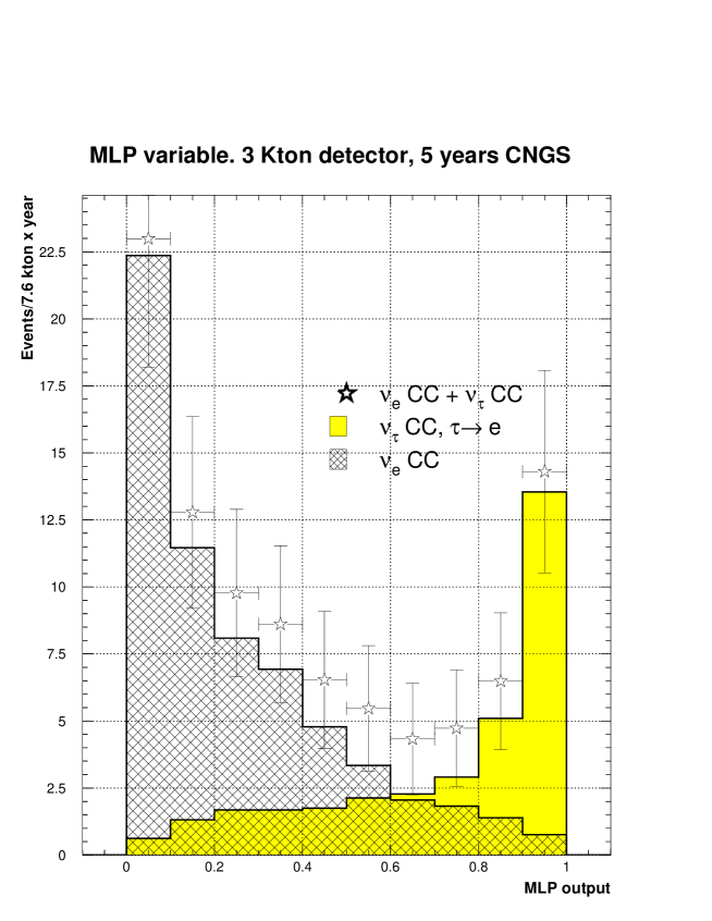
Figure 8: Multi-layer perceptron output for $\nu_{\tau}$CC ($\tau\rightarrow e$) and $\nu_{e}$CC events. We see how signal events accumulate around 1 while background peaks at 0. Only statistical errors are plotted.

Figure 9 shows the number of signal and background expected after 5 years of data taking as a function of the cut in the MLP variable. In figure 10 we represent the probability of an event, falling in a region of the input space characterized by MLP output $>$ cut, to be a signal event (top plot), and the statistical significance as a function of the MLP cut (bottom plot). Background rejection has been optimized since a cut based on the MLP output variable can select regions of complicated topology in the kinematic hyperspace, given that now complex correlations are taken into account (see figure 11).

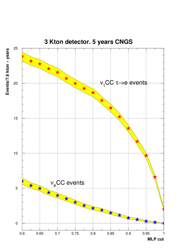
Figure 9: Number of signal and background events after 5 years of running CNGS as a function of the MLP cut. Shadowed zones correspond to statistical errors.

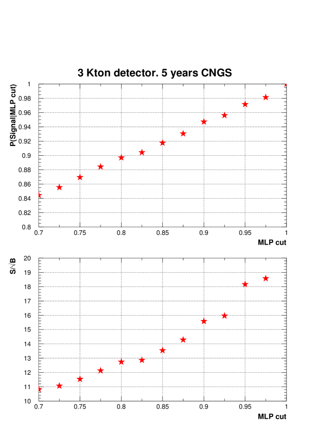
Figure 10: (Top) Probability of an event belonging to a region in input variable space characterized by MLP $>cut$ of being a signal event. (Bottom) Statistical significance of signal events as a function of the cut in MLP.

Selecting MLP $>0.91$ (overall $\tau$ selection efficiency $=25$%), the probability that an event falling in this region is signal amounts to $\sim 0.95$. For 5 years of running CNGS and a 3 kton detector, we expect a total amount of $12.9\pm 0.5$ $\nu_{\tau}$CC ($\tau\rightarrow e$) events and $0.66\pm 0.14$ $\nu_{e}$CC events. Table 4 summarizes as a function of the applied MLP cut the expected number of signal and background events.

If we compare the outcome of this approach with the one obtained in section 4.1.1, we see that for the same $\tau$ selection efficiency, the multi-dimensional likelihood expects $1.1\pm 0.2$ background events. Therefore, for this particular cut, the MLP achieves a 60% reduction in the number of expected $\nu_{e}$ CC events.

	$\nu_{\tau}$CC ($\tau\rightarrow e$)		$\nu_{\tau}$ CC ($\tau\rightarrow e$)
Cuts	Efficiency	$\nu_{e}$CC	$\Delta m^{2}=$
	(%)		$3\times 10^{-3}$ eV2
Initial	100	252	50
Fiducial volume	65	164	33
MLP $>0.70$	42	$4.0\pm 0.4$	$21.4\pm 0.6$
MLP $>0.75$	40	$3.0\pm 0.3$	$19.9\pm 0.6$
MLP $>0.80$	37	$2.1\pm 0.3$	$18.6\pm 0.5$
MLP $>0.85$	33	$1.5\pm 0.2$	$16.4\pm 0.5$
MLP $>0.90$	27	$0.76\pm 0.15$	$13.5\pm 0.5$
MLP $\mathbf{>0.91}$	25	$\mathbf{0.66\pm 0.14}$	$\mathbf{12.9\pm 0.5}$
MLP $>0.95$	19	$0.28\pm 0.09$	$9.6\pm 0.4$
MLP $>0.98$	12	$0.09\pm 0.05$	$5.8\pm 0.3$

Table 4: Expected number of background and signal events when a multi-layer perceptron function is used as the unique discriminant. Numbers are normalized to 5 years running of CNGS. Errors in the number of events expected are of statistical nature.

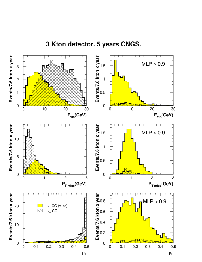
Figure 11: Kinematic variables before (left histograms) and after (right histograms) cuts are applied based on the MLP output. We see how the MLP has learnt that signal events favour low $E_{visible}$, high $P_{T}^{miss}$ and low $\rho_{l}$ values.

As we did for the Fisher method, we studied if the sensitivity given by the MLP increases when a larger number of input variables is used. Even though the number of complex correlations among variables is larger, the change in the final sensitivity is negligible. Once again, all the discrimination power is provided by $E_{visible}$, $P_{T}^{miss}$ and $\rho_{l}$. The surviving background can not be further reduced by increasing the dimensionality of the problem.

Since an increase on the number of input variables does not improve the discrimination power of the multi-layer perceptron, we tried to enhance signal efficiency following a different approach: optimizing the set of input variables by finding new linear combinations of the original ones (or functions of them like squares, cubes, etc).

To this purpose, using the fast computation capabilities of the Fisher method, we can operate in a systematic way in order to find the most relevant feature variables. Starting from an initial set of input variables, the algorithm described in [31] tries to gather all the discriminant information in an smaller set of optimized variables. These last variables are nothing but successive Fisher functions of different combinations of the original ones. In order to allow not only linear transformations, we can add non-linear functions of the kinematic variables like independent elements of the initial set.

We performed an analysis similar to the one described in [31], using 5 initial kinematic variables ($E_{vis}$, $P_{T}^{miss}$, $\rho_{l}$, $P_{T}^{lep}$ and $E_{lep}$) plus their cubes and their exponentials (in total 15 initial variables). At the end, we chose a smaller subset of six optimized Fisher functions that we use like input features variables for a new multi-layer perceptron.

The MLP analysis with six Fisher variables does not enhance the oscillation search sensitivity that we got with the three usual variables $E_{vis}$, $P_{T}^{miss}$and $\rho_{l}$. We therefore conclude that neither the increase on the number of features variables nor the use of optimized linear combinations of kinematic variables as input, enhances the sensitivity provided by the MLP.

The application of statistical techniques able to find complex correlations among the input variables is the only way to enhance background rejection capabilities. In this respect, neural networks are an optimal approach.

4.2.2 Self Organizing Neural Networks: LVQ Network

A self-organizing (SO) network operates in a different way than a multi-layer perceptron does. These networks have the ability to organize themselves according to the “natural structure” of the data. They can learn to detect regularities and correlations in their input and adapt their future response to that input accordingly. A SO network usually has, besides the input, only one layer of neurons that is called competitive layer (see figure 12). Neurons in the competitive layer are able to learn the structure of the data following a simple scheme called competitive self-organization (see [27]), which “moves” the basic units (neurons) in the competitive layer in such a way that they imitate the natural structure of the data.

Competitive self-organization is an unsupervised learning algorithm, however for classification purposes one can improve the algorithm with supervised learning in order to fine tune final positions of the neurons in the competitive layer. This is called learning vector quantization (LVQ) (for further details refer to [25, 27]). An important difference with respect to the multi-layer perceptron approach is that in LVQ we always get a discrete classification, namely, an event is always classified in one of the classes. The only thing one can estimate is the degree of belief in the LVQ choice.

Figure 12: Schematic diagram of the general topology for a self-organized neural network. Neurons in the competitive layer are connected with each one of the input nodes.

LVQ Network for $\nu_{\tau}$ Appearance Search

We use once more $E_{visible}$, $P_{T}^{miss}$ and $\rho_{l}$ as discriminating variables inside the input layer. A LVQ network with 10 neurons has been trained with samples of 2500 events for both signal and background. Given that, before any cut, a larger background sample is expected, we have chosen an asymmetric configuration for the competitive layer. Out of 10 neurons, 6 were assigned to recognize background events, and the rest were associated to the signal class. After the neurons are placed by the training procedure, the LVQ network is fed with a larger and statistically independent data sample consisting of 6000 signal and background events. The output provided by the network is plotted in figure 13. We see how events are classified in two independent classes: signal like events (labeled with 2) and background like ones (labeled with 1). 68% of $\nu_{\tau}$CC ($\tau\rightarrow e$) events and 10% of $\nu_{e}$CC events, occurring in fiducial volume, are classified as signal like events. This means a $\tau$ efficiency around 45% with respect to the tau events generated in active LAr. For the same $\tau$ efficiency, the multi-layer perceptron only misclassified around 8% of $\nu_{e}$CC events.

Several additional tests have been performed with LVQ networks, by increasing the number of input variables and/or the number of neurons in the competitive layer. However, we observed no improvement on the separation capabilities. For instance, a topology with 16 feature neurons in the competitive layer and 4 input variables (we add the transverse lepton momentum) leads to exactly the same result.

The simple geometrical interpretation of this kind of neural networks supports our statement that the addition of new variables to the original set {$E_{visible}$, $P_{T}^{miss}$ , $\rho_{l}$} does not enhance the discrimination power: the bulk of signal and background events are not better separated when we increment the dimensionality of the input space.

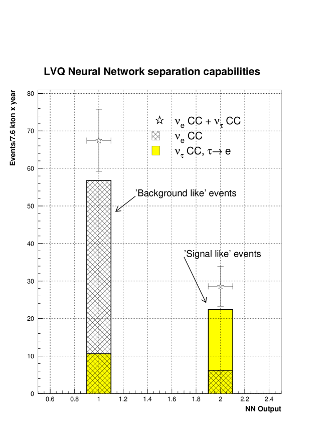
Figure 13: LVQ neural network separation capabilities. In competitive self-organized networks a discrete decision is always issued: signal like events are labeled with 2 and background like with 1.

Combining MLP with LVQ

We have seen that LVQ networks returns a discrete output. The whole event sample is classified by the LVQ in two classes: signal-like and background-like. We can use the classification of a LVQ as a pre-classification for the MLP. A priori, it seems reasonable to expect an increase on the oscillation search sensitivity if we combine the LVQ and MLP approaches. The aim is to evaluate how much additional background rejection, from the contamination inside the signal-like sample, can be obtained by means of a MLP.

We present in figure 14 the MLP output for events classified as signal-like by the LVQ network (see figure 13). Applying a cut on the MLP output such that we get $12.9$ signal events (our usual reference point of 25% $\tau$ selection efficiency), we get $0.82\pm 0.19$ background events, similar to what was obtained with the MLP approach alone. This outcome conclusively shows that, contrary to our a priori expectations, an event pre-classification, by means of a learning vector quantization neural network, does not help improving the discrimination capabilities of a multi-layer perceptron.

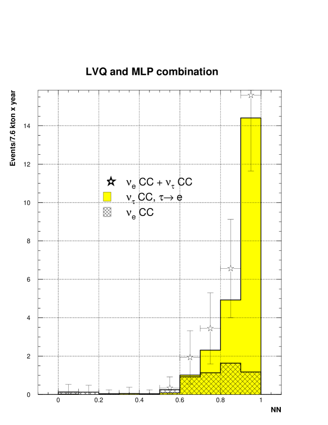
Figure 14: LVQ and MLP networks combined. Distributions are given in the continuous MLP variable. Only events labeled by LVQ with 2 (signal like) have been used for the analysis.

5 $\nu_{\tau}$ Discovery Potential

We have studied several pattern recognition techniques applied to the particular problem of searching for $\nu_{\mu}\rightarrow\nu_{\tau}$ oscillations. Based on discovery criteria, similar to the ones proposed in [32] for statistical studies of prospective nature, we try to quantify how much the statistical relevance of the $\tau$ signal varies depending on the statistical method used.

We define $\mu_{S}$ and $\mu_{B}$ as the average number of expected signal and background events, respectively. With this notation, we impose two conditions to consider that a signal is statistically significant:

1. We require that the probability for a background fluctuation, giving a number of events equal or larger than $\mu_{S}+\mu_{B}$, be smaller than $\epsilon$ (where $\epsilon$ is $5.733\times 10^{-7}$, the usual $5\sigma$ criteria applied for Gaussian distributions).

2. We also set at which confidence level $(1-\delta)$, the distribution of the total number of events with mean value $\mu_{S}+\mu_{B}$ fulfills the background fluctuation criteria stated above.

For instance, if $\delta$ is $0.10$ and $\epsilon$ is $5.733\times 10^{-7}$, we are imposing that $90\%$ of the times we repeat this experiment, we will observe a number of events which is $5\sigma$ or more above the background expectation.

For all the statistical techniques used, we fix $\delta$=$0.10$ and $\epsilon$=$5.733\times 10^{-7}$. In this way we can compute the minimum number of events needed to establish that, in our particular example, a direct $\nu_{\mu}\rightarrow\nu_{\tau}$ oscillation has been observed.

In table 5 we compare the number of signal and background events obtained for the multi-layer perceptron and the multi-dimensional likelihood approaches after 5 years of data taking with a 3 kton detector. We also compare the minimum exposure needed in order to have a statistically significant signal. The minimum exposure is expressed in terms of a scale factor $\alpha$, where $\alpha=1$ means a total exposure of $11.75$ kton$\times$year. For the multi-layer perceptron approach ($\alpha=0.86$), a statistically significant signal can be obtained after a bit more than four years of data taking. On the other hand, the multi-dimensional likelihood approach requires 5 full years of data taking. Therefore, when applied to the physics quest for neutrino oscillations, neural network techniques are more performant than classic statistical methods.

	Multi-layer	Multi-dimensional
	Perceptron	Likelihood
# Signal	12.9	12.9
# Background	0.66	1.1
$\alpha$ factor	0.86	1.01

Table 5: Number of signal and background events for the multi-layer perceptron and the multi-dimensional likelihood approaches. Numbers are normalized to 5 years of data taking in shared CNGS running mode and a 3 kton detector configuration. The last row displays the scale factor $\alpha$ needed to compute the minimum exposure fulfilling the discovery criteria described in the text.

6 Conclusions

We have considered the general problem of $\nu_{\mu}\to\nu_{\tau}$ oscillation search based on kinematic criteria to assess the performance of several statistical pattern recognition methods.

Two are the main conclusions of this study:

• An optimal discrimination power is obtained using only the following variables: $E_{visible}$, $P_{T}^{miss}$ and $\rho_{l}$ and their correlations. Increasing the number of variables (or combinations of variables) only increases the complexity of the problem, but does not result in a sensible change of the expected sensitivity.

• Among the set of statistical methods considered, the multi-layer perceptron offers the best performance.

As an example, we have considered the case of the CNGS beam and $\nu_{\tau}$ appearance search (for the $\tau\to e$ decay channel) using a very massive (3 kton) Liquid Argon TPC detector. Figure 15 compares the discrimination capabilities of multi-dimensional likelihood and multi-layer perceptron approaches. We see that, for the low background region, the multi-layer perceptron gives the best sensitivity. For instance, choosing a $\tau$ selection efficiency of 25% as a reference value, we expect a total of $12.9\pm 0.5$ $\nu_{\tau}$CC ($\tau\rightarrow e$) signal and $0.66\pm 0.14$ $\nu_{e}$CC background. Compared to multi-dimensional likelihood predictions, this means a 60% reduction on the number of expected background events. Hence, using a multi-layer perceptron, fours years of data taking will suffice to get a statistically significant signal, while five years are needed when the search approach is based on a multi-dimensional likelihood.

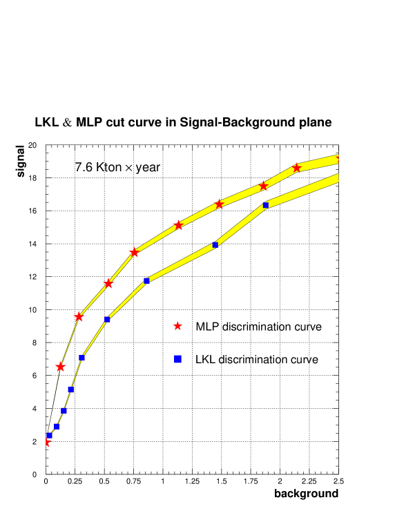
Figure 15: Multi-layer perceptron vs multi-dimensional likelihood. We assume a 7.6 Kton$\times$year exposure. The shadowed area shows the statistical error.

References

- [1] Y. Fukuda et al., [Super-Kamiokande Collaboration], Phys. Rev. Lett. 81 (1998) 1562.
- [2] Q. R. Ahmad et al. [SNO Collaboration], Phys. Rev. Lett. 89 (2002) 011301.
-
[3]
A. Salam, 1969. Proc. of the 8th Nobel Symposium on ‘Elementary particle theory, relativistic groups and analyticity’, Stockholm, Sweden, 1968, edited by N. Svartholm, p.367-377.
S. Weinberg, Phys. Rev. Lett. 19 (1967) 1264.
S. L.Glashow, Nucl. Phys. 22 (1961) 579. - [4] M. H. Ahn et al. [K2K Collaboration], Phys. Rev. Lett. 90 (2003) 041801.
- [5] K. Eguchi et al. [KamLAND Collaboration], Phys. Rev. Lett. 90 (2003) 021802.
-
[6]
D. L. Wark, Nucl. Phys. Proc. Suppl. 117 (2003) 164.
A. Yu. Smirnov, hep-ph/0402264. 2nd Int. Workshop on Neutrino oscillations in Venice (NOVE) December 2003, Venice, Italy. - [7] P. Zucchelli, CERN-EP-2001-056, Jul 2001. 8pp; hep-ex/0107006.
- [8] S. Geer, Phys. Rev. D 57 (1998) 6989.
-
[9]
A. De Rújula, M. B. Gavela, P. Hernández, Nucl. Phys. B 547 (1999) 21.
V. D. Barger, S. Geer, R. Raja and K. Whisnant, Phys. Rev. D 62 (2000) 013004.
A. Cervera et al., Nucl. Phys. B 579 (2000) 17.
A. Bueno, M. Campanelli and A. Rubbia, Nucl. Phys. B 589 (2000) 577.
A. Bueno, M. Campanelli, S. Navas-Concha and A. Rubbia, Nucl. Phys. B 631 (2002) 239. - [10] Y. Ashie et al., [Super-Kamiokande Collaboration], hep-ex/0404034.
- [11] G. Acquistapace et al., CERN-98-02; R. Baldy et al., CERN-SL-99-034-DI.
- [12] F. Arneodo et al. [ICARUS Collaboration], “The ICARUS experiment, a second-generation proton decay experiment and neutrino observatory at the Gran Sasso laboratory”, CERN/SPSC 2002-027 (SPSC-P-323), Aug. 2002.
- [13] M. Guler et al. [OPERA Collaboration], CERN/SPSC 2000-028, SPSC/P318, LNGS P25/2000.
- [14] J. Altegoer et al. [NOMAD Collaboration], Nucl. Instrum. Meth. A 404 (1998) 96.
- [15] E. Eskut et al. [CHORUS Collaboration], Nucl. Instrum. Meth. A 401 (1997) 7.
- [16] C. H. Albright and R. E. Shrock, Phys. Lett. B 84 (1979) 123.
- [17] J. Altegoer et al. [NOMAD Collaboration], Phys. Lett. B 431 (1998) 219.
- [18] P. Astier et al. [NOMAD Collaboration], Phys. Lett. B 453 (1999) 169.
- [19] P. Astier et al. [NOMAD Collaboration], Nucl. Phys. B 611 (2001) 3.
- [20] A. Rubbia, talk at the First International Workshop on Neutrino-Nucleus Interactions in the Few GeV Region (Nuint 01), December 2001, KEK, Tsukuba, Japan.
- [21] See http://www.fluka.org/ for further details.
- [22] P. Aprili et al. [ICARUS Collaboration], LNGS-EXP 13/89 add. 3/03 CERN/SPSC 2003-030 (SPSC-P-323-Add.1).
- [23] F. Arneodo et al. [ICANOE Collaboration], LNGS P21/99 INFN/AE-99-17 CERN/SPSC 99-25 SPSC/P314.
- [24] G. Cowan, “Statistical data analysis”. Oxford university Press, 1998.
- [25] C.M. Bishop, “Neural Networks for Pattern Recognition”. Oxford University Press, 1995.
- [26] S. Haykin, “Neural Networks: A comprehensive foundation”. Prentice Hall, 1999.
- [27] C. Peterson, T. Rögnvaldsson, “An introduction to Artificial Neural Networks”. 1991 CERN School Of Computing Proceedings, CERN 92-02.
- [28] Ll. Ametller et al., Phys. Rev. D 54 (1996) 1233.
- [29] P. Chiappetta et al., Phys. Lett. B 332 (1994) 219.
-
[30]
PAW neural network interface. MLPfit package (version 1.33).
http://home.cern.ch/schwind/MLPfit.html. - [31] B.P. Roe, “Event selection using an extended Fisher discriminant method”. Talk given at PHYSTAT2003, SLAC, Stanford.
- [32] J.J. Hernández, S. Navas, P. Rebecchi, Nucl. Instrum. Meth. A 372 (1996) 293.