Saturation and forward jets at HERA

Abstract

We analyse forward-jet production at HERA in the framework of the Golec-Biernat and Wüsthoff saturation models. We obtain a good description of the forward-jet cross-sections measured by the H1 and ZEUS collaborations in the two-hard-scale region ($k_{T}\!\sim\!Q\!\gg\!\Lambda_{QCD}$) with two different parametrizations with either significant or weak saturation effects. The weak saturation parametrization gives a scale compatible with the one found for the proton structure function $F_{2}$. We argue that Mueller-Navelet jets at the Tevatron and the LHC could help distinguishing between both options.

I Introduction

The saturation regime describes the high-density phase of partons in perturbative QCD. It may occur for instance when the Balitsky-Fadin-Kuraev-Lipatov (BFKL) QCD evolution equation bfkl goes beyond some energy related to the unitarity limit GLR ; qiu ; venugopalan ; Balitsky:1995ub ; levinbar ; Mueller:2002zm . On a phenomenological ground, a well-known saturation model golec by Golec-Biernat and Wüsthoff (GBW) gives a parametrization of the proton structure functions already in the HERA energy range. It provides a simple and elegant formulation of the transition to saturation. However, there does not yet exist a clear confirmation of saturation since the same data can well be explained within the conventional perturbative QCD framework dglap .

In fact, the study of the proton structure functions is a one-hard-scale analysis since their QCD properties are dominated by the evolution from a soft scale (the proton scale) to the hard scale of deep inelastic scattering. In order to favor the evolution at fixed transverse scale, which is expected to lead more directly to saturation, it seems interesting to focus on two-hard-scale processes such as forward-jet production at HERA, in the region where the transverse momentum of the jet $k_{T}$ is of the order of the virtuality of the photon $Q^{2}$ and where the rapidity interval for soft radiation is large. This kinematical configuration which was already proposed dis for testing the BFKL evolution is thus also a good testing ground for saturation. The goal of our paper is then to formulate and study the extension of the GBW model to forward jets at HERA.

Among the physics questions that we want to raise, we analyse whether saturation effects can be sizeable in forward jets at HERA and whether they are compatible or not with the GBW parametrization of $F_{2}.$ More generally, we would like to compare potential saturation effects in one-scale and two-scale processes. Indeed, in the two-scale process initiated by $\gamma^{*}\gamma^{*}$ scattering, it has been suggested levin that the saturation scale could be different and in fact quite larger than the one of deep inelastic scattering. However, another study of $\gamma^{*}\gamma^{*}$ scattering sticks to the same saturation scale as for $\gamma^{*}p$ scattering motyka . We will discuss this point with forward-jet data which have better statistics and wider kinematical range than $\gamma^{*}\gamma^{*}$ scattering. If the saturation scale is universal as assumed in motyka , then one should not expect to see stronger saturation effects in forward-jet data than for $F_{2};$ however if the saturation scale is higher for processes initiated by two hard scales as proposed in levin , saturation effects could be more important.

For HERA, the existence of two different saturation scales for one or two hard-scale processes would be an interesting feature. This study is also of interest in the prospect of Mueller-Navelet jets navelet at the Tevatron and the LHC where saturation with two hard scales could play a bigger role.

The plan of the paper is the following. In Section 2, we formulate the extension of the GBW model for forward jets. In Section 3, we present the fitting method and give the results of the fits together with several tests of the two saturation solutions that we obtain. Section 4 is devoted to a discussion of our results and to predictions for Mueller-Navelet jets at hadron colliders that could discriminate between both solutions.

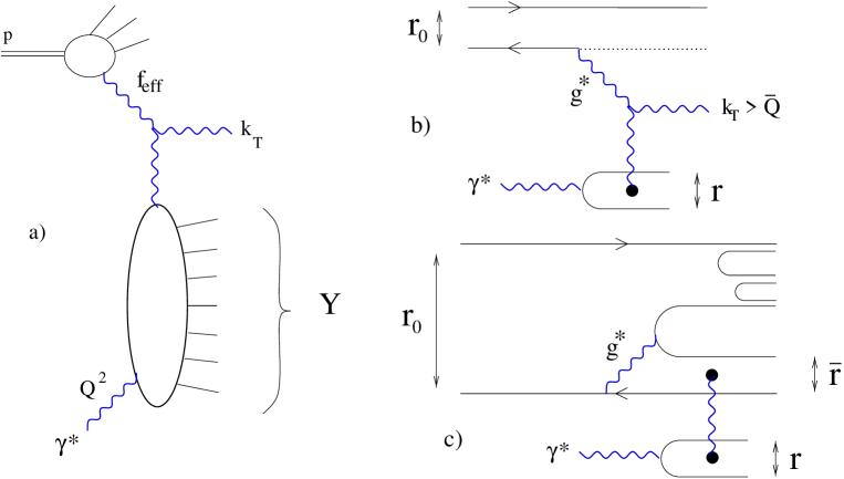
Figure 1: Forward-jet production in partonic and dipole representations. Fig 1a: Forward jets at HERA. Fig 1b: Forward jet in $\gamma^{*}\!-\!onium$ scattering in the partonic representation (at 1st order, i.e. with only one gluon exchanged). Fig 1c: Forward jet in $\gamma^{*}\!-\!onium$ scattering in the dipole representation. $Y:$ rapidity gap between the two hard probes. $k_{T}\!>\!\bar{Q}:$ jet tranverse momentum lower bound. $Q:$ virtuality of the photon. The gluon-dipole couplings are sketched by black points.

II Formulation

The original GBW model provides a simple formulation of the dipole-proton cross-section in terms of a saturation scale $R_{0}(Y)\!\sim\!e^{-\frac{\lambda}{2}\left(Y-Y_{0}\right)}$ where $Y\!=\!\log{1/x}$ is the total rapidity, $\lambda$ is the intercept and $Y_{0}$ sets the absolute value. Varying $Q,$ $QR_{0}\!\gg\!1$ corresponds to the dilute limit while when $QR_{0}\!<\!1$, the dipole-proton cross-section saturates to a finite limit $\sigma_{0}$. In two-hard-scale problems, one has now to deal with dipole-dipole cross-sections which require an extension motyka of the GBW parametrization. In the case of forward jets, one has to combine the dipole-dipole cross-section with an appropriate definition of the coupling of this cross-section to the forward jet. This has been proposed in us . We shall use this coupling in the analysis of forward jets at HERA.

The QCD cross-section for forward-jet production in a lepton-proton collision reads

$$\frac{d^{(4)}\sigma}{dxdQ^{2}dx_{J}dk_{T}^{2}}=\frac{\alpha}{\pi xQ^{2}}\ f_{eff}(x_{J},k_{T}^{2})\left\{{\left({\frac{d\sigma_{T}}{dk_{T}^{2}}+\frac{d\sigma_{L}}{dk_{T}^{2}}}\right)}(1-y)+\frac{d\sigma_{T}}{dk_{T}^{2}}\frac{y^{2}}{2}\right\},$$ (1)

where $x$ and $y$ are the usual kinematic variables of deep inelastic scattering, $Q^{2}$ is the virtuality of the photon with longitudinal (L) and transverse (T) polarization, and $x_{J}$ is the jet longitudinal momentum fraction with respect to the proton. $d\sigma_{T,L}/dk_{T}^{2}$ are the photon-parton hard differential cross-sections for the production of a forward (gluon) jet with transverse momentum $k_{T}\!\gg\!\Lambda_{QCD}$. The effective parton distribution function $f_{eff}$ has the following expression

$$f_{eff}(x_{J},k_{T}^{2})=g(x_{J},k_{T}^{2})+\frac{4}{9}{\left({q(x_{J},k_{T}^{2})+\bar{q}(x_{J},k_{T}^{2})}\right)}\ ,$$ (2)

where $g$ (resp. $q$, $\bar{q}$) are the gluon (resp. quark, antiquark) structure functions in the incident proton. $k_{T}^{2}$ is chosen as the QCD factorization scale.

Properly speaking, the forward-jet cross-section (1) is the leading $\log{(1/x)}$ expression when one uses the BFKL formulation of $d\sigma_{T,L}/dk_{T}^{2}.$ Let us show how one can extend this formalism when saturation corrections are present, e.g. in the framework of the GBW model. The differential hard cross-section reads

$$\frac{d\sigma_{T,L}}{dk_{T}^{2}}=\left.-\frac{\partial\sigma_{T,L}}{\partial\bar{Q}^{2}}(Q^{2},\bar{Q}^{2})\right|_{\bar{Q}=k_{T}}$$ (3)

where $\sigma_{T,L}$ are the cross-sections for the production of a forward jet with transverse momentum larger than $\bar{Q},$ expressed in the dipole framework by us

$$\sigma_{T,L}(Q^{2},\bar{Q}^{2})=\frac{\pi^{2}\sigma_{0}}{2}\int d^{2}r\ d^{2}\bar{r}\ \phi^{\gamma}_{T,L}(r,Q^{2})\ \phi^{J}(\bar{r},\bar{Q}^{2})\left\{1-\exp{{\left({-\frac{r_{eff}^{2}(r,\bar{r})}{4R_{0}^{2}(Y)}}\right)}}\right\}\ .$$ (4)

$\sigma_{0}$ times the term in brackets in formula (4) is the GBW dipole-dipole cross-section.

$$R^{2}_{0}(Y)=\frac{1}{Q^{2}_{0}}\ e^{-\lambda\left(Y-Y_{0}\right)}$$ (5)

is the saturation radius redefined for the forward jet case, where $Y\!=\!\log{x_{J}/x}$ is the rapidity interval available for the forward-jet cross-section (see Fig 1), $\lambda$ is the saturation intercept and $Y_{0}$ is a parameter defining the rapidity for which $R_{0}(Y_{0})\!=\!1/Q_{0}\!\equiv\!1$ GeV^-1. $\sigma_{0}$ is the value at which the dipole-dipole cross-section saturates. The effective radius $r_{eff}^{2}(r,\bar{r})$ is defined through the elementary dipole-dipole cross-section given by the two-gluon exchange mueller

$$\sigma_{dd}(r,\bar{r})=\int d^{2}kf^{0}(k^{2},r)f^{0}(k^{2},\bar{r})=2\pi\alpha^{2}_{s}r^{2}_{<}{\left({1+\ln\frac{r_{>}}{r_{<}}}\right)}\equiv 2\pi\alpha^{2}_{s}r^{2}_{eff}(r,\bar{r})\ ,$$ (6)

where $r^{2}_{<}$ (resp. $r^{2}_{>}$) is $\min{(r,\bar{r})}$ (resp. $\max{(r,\bar{r})}$), $\alpha_{s}$ is QCD the coupling constant and $f^{0}(k^{2},r)\equiv 2\alpha_{s}(1-J_{0}(kr))/k^{2}$ is the dipole-gluon coupling. The functions $\phi^{\gamma}_{T,L}(r,Q^{2})$ and $\phi^{J}(\bar{r},\bar{Q}^{2})$ express the couplings to the virtual photon and to the jet. $\phi^{\gamma}_{T,L}(r,Q^{2})$ is the known squared QED wavefunction bjorken of a photon in terms of $q\bar{q}$.

In equation (4), the definition of $\phi^{J}(\bar{r},\bar{Q}^{2})$ associated with a forward jet with transverse momentum $k_{T}\!>\!\bar{Q}$ requires more care. The gluon jet is colored while the associated dipole $\bar{r}$ is not, see Fig.1c. $\phi^{J}$ is obtained by taking advantage of the equivalence between the partonic and dipole formulations of forward-jet production when the jet is emitted off an onium (see Fig 1b-1c, where the size of the incident onium is denoted $r_{0}$). Let us sketch the derivation of $\phi^{J}(\bar{r},\bar{Q}^{2}).$ Assuming the condition $1\,GeV^{-1}\!\gg\!r_{0}\!\gg\!1/\bar{Q},$ the onium is small enough to allow for a perturbative QCD calculation but large enough with respect to the inverse transverse momentum of the forward jet. At lowest pertubative order, the coupling of the system onium-jet to the gluon (interacting with the target photon) reads munier ; robi ; us :

$$\alpha_{s}\log\frac{1}{x_{J}}\int\frac{d^{2}\vec{k}_{T}}{\pi\vec{k}_{T}^{2}}\theta(\vec{k}_{T}^{2}-\bar{Q}^{2})f^{0}(|\vec{k}+\vec{k}_{T}|^{2},r_{0})\approx\left\{2\alpha_{s}\log\frac{1}{x_{J}}\log{\bar{Q}r_{0}}\right\}\int d^{2}\bar{r}\ \frac{\bar{Q}}{2\pi\bar{r}}\ J_{1}(\bar{Q}\bar{r})\ f^{0}(k^{2},\bar{r})\ .$$ (7)

The function $f^{0}(k^{2},\bar{r})$ factorizes as part of the dipole-dipole cross-section (6). The factor in brackets in (7) is the first order contribution of the Dokshitzer-Gribov-Lipatov-Altarelli-Parisi (DGLAP) gluon ladder dglap , at the Double Leading Log (DLL) approximation. QCD factorization thus implies that it is included in the structure function of the incident particule. In the case of a proton it is absorbed in $f_{eff},$ see formula (2), by a redefinition of the factorization scale. Therefore, the remaining term gives

$$\phi^{J}(\bar{r},\bar{Q}^{2})\equiv\frac{\bar{Q}}{2\pi\bar{r}}\ J_{1}(\bar{Q}\bar{r})\ .$$ (8)

Note that $\phi^{J}$ is an effective distribution that comes out from the calculation rather than a probability distribution as for $\phi^{\gamma}_{T,L}.$

Inserting in formula (4) the known Mellin transforms $\tilde{\phi}(\tau)\!=\!\int d^{2}r\ (r^{2}Q^{2})^{1-\tau}\phi(r,Q^{2}):$

$$\tilde{\phi}^{J}(\tau)=2^{2-2\tau}\frac{\Gamma(2-\tau)}{\Gamma(\tau)}\ ,\hskip 28.45274pt\tilde{\phi}^{\gamma}_{T,L}(\gamma)=\frac{2N_{c}\alpha}{\pi}\sum_{q}e_{q}^{2}\frac{1}{4^{\gamma}\gamma}\frac{\Gamma^{2}(1+\gamma)\Gamma^{2}(1-\gamma)\Gamma^{2}(2-\gamma)}{\Gamma(2-2\gamma)\Gamma(2+2\gamma)(3-2\gamma)}{\left({\begin{array}[]{cc}(1+\gamma)(2-\gamma)\\ 2\gamma(1-\gamma)\end{array}}\right)}$$ (9)

and after straightforward transformations we can express our results in a double Mellin-transform representation:

$$\frac{d\sigma_{T,L}}{dk_{T}^{2}}=\frac{\pi^{2}}{8Q^{2}k_{T}^{2}R_{0}^{2}(Y)}{\int\frac{d\gamma}{2i\pi}}\ \tilde{\phi}^{\gamma}_{T,L}(\gamma)(4Q^{2}R_{0}^{2})^{\gamma}{\int\frac{d\tau}{2i\pi}}\ \tilde{\phi}^{J}(1\!-\!\tau)(4k_{T}^{2}R_{0}^{2})^{-\tau}\left\{\tau\tilde{\sigma}(\tau,\gamma)\right\}\ ,$$ (10)

$$0<Re(\tau),\;Re(\gamma),\;Re(\gamma-\tau)<1\ \ ,$$

where

$$\tilde{\sigma}(\tau,\gamma)\equiv\sigma_{0}\int du^{2}\int d\bar{u}^{2}u^{2\gamma-4}\bar{u}^{-2\tau-2}{\left({1-e^{-r_{eff}^{2}(u,\bar{u})}}\right)}=\sigma_{0}\frac{2\Gamma{(\gamma-\tau)}}{1+\tau-\gamma}\int_{0}^{\infty}du\ u^{-2\tau-1}\left[r_{eff}^{2}(1,u)\right]^{1+\tau-\gamma}\ .$$ (11)

Using (6), one finally gets

$$\tilde{\sigma}(\tau,\gamma)=\sigma_{0}\ \frac{2\Gamma{(\gamma-\tau)}}{1+\tau-\gamma}\ \left\{\Psi(1,3+\tau-\gamma,2\tau)+\Psi(1,3+\tau-\gamma,2-2\gamma)\right\}\ ,$$ (12)

where the confluent hypergeometric function of Tricomi $\Psi(1,a,b)$ can be expressed prud in terms of incomplete Gamma functions.

Note that, expanding the exponential function in the GBW dipole-dipole cross-section in (4), it is possible to single out order by order the contribution of $r_{eff}^{2n}$ in formula (10):

$$\tilde{\sigma}^{(n)}(\tau,\gamma)=2\sigma_{0}\frac{(-1)^{n-1}}{n!}\ 2i\pi\delta(\gamma-\tau+n-1)\left\{\Psi(1,3+\tau-\gamma,2\tau)+\Psi(1,3+\tau-\gamma,2-2\gamma)\right\}\ .$$ (13)

There is an interesting physical interpretation of this expansion. $\tilde{\sigma}^{(1)}$ corresponds to the dilute limit of the GBW formula. Taking also into account $\tilde{\sigma}^{(2)}$ can be interpreted as saturation a la Gribov-Levin-Ryskin GLR , i.e. $\sim\!r_{eff}^{2}\!-\!r_{eff}^{4}/8R^{2}_{0}(Y)$. Note also that formulae (10,11) can also be used with the other models for $r^{2}_{eff}$ proposed in the literature motyka .

III Fitting forward jets

For the fitting procedure, we will use a method allowing for a direct comparison of the data with theoretical predictions. This method has already been applied jets for a BFKL parametrization of the same $d\sigma/dx$ data at HERA. We shall extend this method to the GBW parametrization (cf. Eq.(10)).

The published data depend on kinematical cuts (see h199 ; ze99 ) which are modeled by bin-per-bin correction factors that multiply the theoretical cross-sections. The details of the method are as follows: i) for each $x$-bin, one determines cont the average values of $Q^{2}$, $x_{J}$, $k_{T}$ from a reliable Monte-Carlo simulation of the cross-sections using the Ariadne program ariadne ; ii) one chooses a set of integration variables for $d^{(4)}\sigma$ (see (1)) in such a way to match closely the experimental cuts and minimize the variation of the cross-sections over the bin size, the convenient choice of bins for forward jets jets is

$$\frac{d\sigma}{dx}=\int\left[Q^{6}\frac{d^{(4)}\sigma}{dxdQ^{2}dx_{J}dk_{T}^{2}}\right]\times\Delta\left(\frac{1}{Q^{2}}\right)\Delta x_{J}\Delta\left(\frac{k_{T}^{2}}{Q^{2}}\right)$$ (14)

(note the choice of the variable $k_{T}^{2}/Q^{2}$ which is well-suited for the study of two-scale processes); iii) one fixes the correction factors due to the experimental cuts for each $x$-bin by a random simulation of the kinematic constraints with no dynamical input. The list of correction factors for the H1 and ZEUS sets of data h199 ; ze99 and more details on the method are given in jets .

Using these correction factors, we perform a fit of formulae (1) to the H1 and ZEUS data using the GBW parametrization (10-12). The free parameters are the saturation scale parameters $\lambda$ and $Y_{0}$ (see (5)) and the normalizations which we keep independent for H1 and ZEUS. Note that they are related to the dimensionless factors $\sigma_{0}Q_{0}^{2}$. We also make the slight modification $\sigma_{0}\!\rightarrow\!\alpha_{S}^{2}(k_{T}^{2})\ \sigma_{0}$ with $\alpha_{S}$ running at one loop with 4 active flavours and $\Lambda_{QCD}=220$ MeV. Indeed, it is known that leading-order BFKL fits are better when the coupling constant in the overall factor is running. It turns out that with our GBW parametrization, the effect is much smaller than in the BFKL case as will be discussed later on. The obtained values of the parameters and the $\chi^{2}$ of the fits are given in Table I and the resulting cross-sections displayed in Fig. 2. We obtain two different solutions which can be characterised by different strength of saturation effects. The $\chi^{2}$ per dof is quite good (we use only statistical errors to perform the fit) in both cases. The two solutions show similar $\chi^{2}$ values and resulting cross-sections and we chose to plot only the solution with higher saturation in Fig. 2 (1st line of table I, the other solution would be indistinguishable on that same figure). It displays the result of the fit (full line) together with the contributions of the 1st ($\tilde{\sigma}^{(1)}$, dotted line) and 1st+2nd ($\tilde{\sigma}^{(1)}\!+\!\tilde{\sigma}^{(2)}$, dashed line) orders keeping the values of the parameters found for the full solution. We can see that these orders give distinguishable contributions.

fit	$\lambda$	$Y_{0}$	${\cal N}_{ZEUS}$	${\cal N}_{H1}$	$\chi^{2}(/dof)$
sat.	0.402 $\pm$ 0.036 $\pm$ 0.024	-0.82 $\pm$ 0.36 $\pm$ 0.01	34.3 $\pm$ 8.5 $\pm$ 7.0	31.7 $\pm$ 8.4 $\pm$ 8.7	6.8 (/11)
weak sat.	0.370 $\pm$ 0.032 $\pm$ 0.015	8.23 $\pm$ 0.48 $\pm$ 0.03	1136 $\pm$ 272 $\pm$ 2	1042 $\pm$ 238 $\pm$ 78	8.3 (/11)

Table 1: Results of the fits to the H1/ZEUS data for the GBW model. We find two independent solutions showing either significant (1st line) or only weak (2nd line) saturation parameters (see text). Statistical and systematic errors are indicated in that order for each parameter.

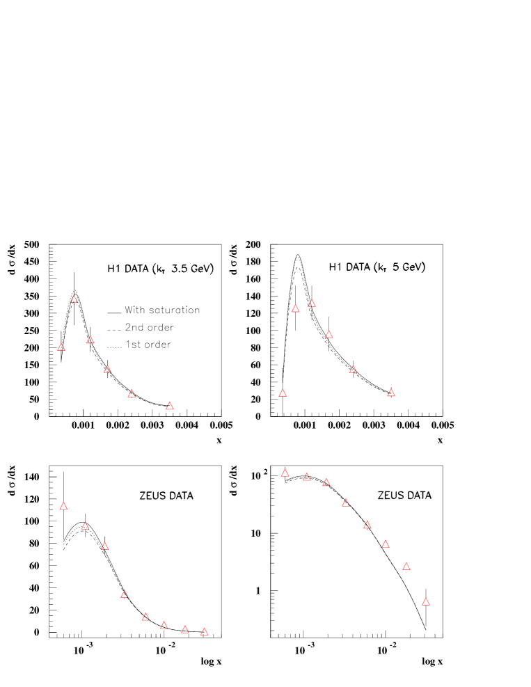
Figure 2: Results of the fit with significant saturation. Upper left: H1 data $k_{T}\!>\!3.5$ GeV, upper right: H1 data $k_{T}\!>\!5$ GeV, lower left and right: ZEUS data in linear and logarithmic (showing the discrepancy at high-$x$) scales. We display the result of the fit in full lines, together with the contribution of 1st and 1st+2nd orders (resp. dotted and dashed lines). The cross-sections are given in nanobarns.

Let us now discuss each solution. The first solution (1st line of Table I) shows a sizeably larger value of $\lambda$ than the $F_{2}$ parametrization golec (cf. $\lambda^{F_{2}}\!=\!0.288$), while the value of $Y_{0}$ is found to be completely different (cf. $Y_{0}^{F_{2}}\!=\!8.1$), leading to more significant saturation effects. The second solution (2nd line of Table I) shows values of $\lambda$ and $Y_{0}$ more compatible with the $F_{2}$ result, even if $\lambda$ remains somewhat larger. The normalizations for H1 and ZEUS data are found to be compatible in both cases. By contrast, the second and absolute $\chi^{2}$ minimum corresponds to fully significant (if not very big) saturation effects. To analyse these features more in detail, we study how the two $\chi^{2}$ minima appear order by order in the expansion of the GBW cross-section using formula (13). In Table II, we show the results of the fits when we truncate the expansion up to first, second and third order. The first order (1st line in Table II), which corresponds to the dilute limit (6), is very close to the 2nd minimum of the full model, showing that it indeed corresponds to weak saturation effects. This also confirms that a mere BFKL description jets of $d\sigma/dx$, similar to the first order approximation (6), fits well the same data. At second order, which corresponds to the GLR version of the model, only one minimum appears and it is closer to the first minimum of Table I. At third order, one recovers the two minima observed with the full model. It is clear that saturation corrections are needed to see the first minima appear and this confirms that it involves significant saturation effects. The weak saturation solution should a priori be present regardless of the number of terms in the expansion, yet it is not the case when the truncation is done at second order. Our interpretation of this feature is that the cross-section (4) is sensitive to large dipoles and to the high$-r_{eff}$ behavior of the truncated dipole-dipole cross-section even when the saturation radius $R_{0}$ is large; this is due to the fluctuations of the jet dipole distribution (8) around its mean value.

order	$\lambda$	$Y_{0}$	${\cal N}_{ZEUS}$	${\cal N}_{H1}$	$\chi^{2}(/dof)$
1	0.372 $\pm$ 0.066 $\pm$ 0.015	-	53.7 $\pm$ 10.9 $\pm$ 7.6	49.3 $\pm$ 11.5 $\pm$ 10.4‘	8.3 (/12)
2 sat	0.452 $\pm$ 0.027 $\pm$ 0.027	-1.71 $\pm$ 0.47 $\pm$ 0.01	20.2 $\pm$ 5.8 $\pm$ 4.9	19.1 $\pm$ 5.2 $\pm$ 6.0	6.8 (/11)
3 (sat.)	0.447 $\pm$ 0.025 $\pm$ 0.026	-1.56 $\pm$ 0.33 $\pm$ 0.02	22.2 $\pm$ 3.0 $\pm$ 5.3	20.9 $\pm$ 2.6 $\pm$ 6.6	6.8 (/12)
3 (weak)	0.374 $\pm$ 0.028 $\pm$ 0.016	6.85 $\pm$ 0.32 $\pm$ 0.12	693 $\pm$ 110 $\pm$ 78	637 $\pm$ 94 $\pm$ 35	8.2 (/12)

Table 2: Results of the fits to the H1/ZEUS data for the GBW models with different truncations. 1st line: 1st order (no saturation), 2nd line: 2nd order ($\sim$ GLR model), 3rd and 4th line: 3rd order with either significant or weak saturation effects.

Let us make some additionnal comments. (i) We used $\alpha^{2}_{S}$ (in the overall factor) running at one loop, and for completion, we checked the results of the fits while keeping $\alpha_{S}$ constant. We find the same quality of the fits but with the effective saturation intercept enhanced by about 30% for the first solution. (ii) We have also studied the other models for effective radii proposed in motyka which lead to fits of the same quality with comparable values for the paramaters. (iii) The physical normalization (see equations (5) and (9)) is ${\cal N}\exp(-\lambda Y_{0})$. We checked that we obtain a set of consistent values around 50 for this physical normalisation for all fits. The disperse values of ${\cal N}$ are compensated by the values of $Y_{0}$.

In Fig 3. we plot the different saturation scales as a function of the physical rapidity interval $Y.$ We also display the saturation scale parametrization obtained by the GBW fit of the proton structure function $F_{2}$ golec . The weak solution is compatible with the one from $F_{2}$ in the physical range from five to ten units in rapidity, the rapidity dependance is however somewhat stronger. This solution favors a universal saturation scale regardless of the presence of a soft scale in the problem, as proposed in motyka where $\gamma^{*}\gamma^{*}$ data are described with the saturation scale obtained from $F_{2}.$ The strong saturation solution gives a curve that lies significantly above the weak and $F_{2}$ curves, indicating that in forward jets, the saturation scale is different and higher than for deep inelastic scattering, as claimed in levin .

At this point it is important to compare the range of $Q_{S}^{2}\!\equiv\!1/R_{0}^{2}$ with the experimental transverse momentum cuts. Notice that these cuts (3.5 and 5 GeV) lie approximately in between the two possible saturation scales. It is thus clear why the saturation effects are different for both solutions.

Figure 3: Saturation scales $\log{Q_{S}^{2}/Q_{0}^{2}}\!=\!\lambda(Y-Y_{0})$. We display the saturation scales for both solutions of our fits (full lines with errors indicated by dashed lines) and compare with the result for $F_{2}$ (dotted line). The weak saturation scale and the one for $F_{2}$ are compatible: lower curves. The other solution lies above, yielding stronger saturation effects.

IV Predictions for the Tevatron and the LHC

The fact that the saturation corrections can be sizeable for two-scale processes suggests that the predictions for related hard cross-sections at hadronic colliders will show striking differences with the weak saturation case. Let us for instance consider the Mueller-Navelet jet production navelet at Tevatron and LHC following the approach of us . Indeed, the Mueller-Navelet jets are directly related to our discussion and, at the level of the two-scale hard cross-section (4), amounts to replacing the photon probe by another forward jet. One writes

$$\sigma_{JJ}(k_{T1},k_{T2},\Delta\eta)=\frac{N_{c}^{2}\sigma_{0}}{16}\int d^{2}r\ d^{2}\bar{r}\ \phi^{J}(r,k_{T1}^{2})\ \phi^{J}(\bar{r},k_{T2}^{2})\left\{1-\exp{{\left({-\frac{r_{eff}^{2}(r,\bar{r})}{4R_{0}^{2}(\Delta\eta)}}\right)}}\right\}\ ,$$ (15)

where $\Delta\eta$ is the rapidity interval between the two jets, and $k_{T1}$ and $k_{T2}$ are their lowest transverse momenta. We thus consider cross-sections integrated over the transverse momenta of the jets with lower bounds $k_{T1}$ and $k_{T2}$. In order to appreciate more quantitatively the influence of saturation, it is more convenient to consider the quantities ${\cal R}_{i/j}$ defined as

$${\cal R}_{i/j}\equiv\frac{\sigma(k_{T1},k_{T2},{\Delta\eta}_{i})}{\sigma(k_{T1},k_{T2},{\Delta\eta}_{j})}\ ,$$ (16)

i.e. the cross-section ratios for two different values of the rapidity interval. These ratios display in a clear way the saturation effects, they also correspond to possible experimental observables if one changes the center-of-mass energy since they can be obtained from measurements at fixed values of the jet light-cone momentum and thus are independent of the parton densities the incident hadrons. Measuring two values of the cross-section for identical jet kinematics and different rapidity intervals $\Delta\eta_{i}$ and $\Delta\eta_{j}$ and dividing them gives the ratio ${\cal R}_{i/j}$. Such observables have actually been used for a study of Mueller-Navelet jets for testing BFKL predictions at the Tevatron goussiou ; jets . However, it is known that hadronization effects play a role in this kind of measurements and have to be taken into account schmidt .

In Fig 4, we show the resulting ratios, when $k_{T1}\!=\!k_{T2}\!\equiv\!k_{T},$ for ${\cal R}_{5/2}$ which corresponds to accessible rapidity intervals at the Tevatron and ${\cal R}_{8/2}$ which corresponds to realistic rapidity intervals for the LHC. The curves are for both saturation solutions together with the prediction obtained from the GBW parametrization of $F_{2}.$ At high scales, both models lead to similar values of ${\cal R}$, larger than the ones extracted us from $F_{2}.$ This reflects the higher saturation intercept systematically found with forward jets in both cases.

A clear difference between the two options (saturation being weak or not) appear in the drop due to saturation which occurs for $k_{T}\!\sim\!Q_{s}.$ For both Tevatron and LHC kinematical configurations, the weak saturation solution would only give effects at rather and probably too low values of $k_{T}$ to be observable. By contrast, the stronger saturation solution would give rise to saturation effects for $k_{T}$ of order $3\ GeV$ for the Tevatron and $30\ GeV$ for the LHC. While the effects could be marginal at Tevatron, the larger value of $k_{T}$ for the LHC provides a way to distinguish between the two solutions and to test the models. Hence the observation or not of saturation effects for Mueller-Navelet jets at LHC is a promising discriminant between the two options.

Figure 4: Cross-section ratios ${\cal R}_{i/j}$. $R_{5/2}$ and $R_{8/2}$ are defined for rapidity intervals 2 and 5 for the Tevatron (3 lower curves), and 2 and 8 for the LHC (3 upper curves). The full lines correspond to the significant saturation solution, first line of Table I. The dashed lines are for the weak saturation solution, second line of Table I. The dotted lines correspond to the saturation parametrization of $F_{2}$.

V Conclusion

Let us briefly summarize the main results of our study. We described the published H1 and ZEUS forward-jet data using a saturation model based on the GBW formalism. We find two possible fits to the data with either significant or weak saturation. The weak saturation solution would be in favor of a universal QCD saturation scale. The solution with significant saturation effects would prove process dependent saturation scales.

Hence the confirmation or not of two different saturation scales, one for one-hard-scale processes (e.g. for $F_{2}$), and one for two-hard-scale processes (e.g. for forward-jets) would suggest interesting theoretical questions, for instance whether the saturation scale is universaly related e.g. to $\Lambda_{QCD}$ or could be related to the hard probes initiating the process.

Both fits lead to different predictions at the Tevatron, and even more different at the LHC where the effect is sizeable for larger jet transverse momentum. The measurement of ${\cal R}_{i/j}$ would imply running the accelerators at different center-of-mass energies. It would allow to test if saturation is stronger for harder processes compared to deep inelastic scattering. It will also be interesting to test the two solutions using the recently presented preliminary H1 and ZEUS forward-jet and forward-pion data, when available.

References

- (1) L. N. Lipatov, Sov. J. Nucl. Phys. 23, (1976) 338; E. A. Kuraev, L. N. Lipatov and V. S. Fadin, Sov. Phys. JETP 45, (1977) 199; I. I. Balitsky and L. N. Lipatov, Sov. J. Nucl. Phys. 28, (1978) 822.
- (2) L. V. Gribov, E. M. Levin and M. G. Ryskin, Phys. Rep. 100, (1983) 1.
- (3) A. H. Mueller and J. Qiu, Nucl. Phys. B268, (1986) 427.
- (4) L. McLerran and R. Venugopalan, Phys. Rev. D49, (1994) 2233; ibid., (1994) 3352; ibid., D50, (1994) 2225; A. Kovner, L. McLerran and H. Weigert, Phys. Rev. D52, (1995) 6231; ibid., (1995) 3809; R. Venugopalan, Acta Phys. Polon. B30, (1999) 3731; E. Iancu, A. Leonidov and L. McLerran, Nucl. Phys. A692, (2001) 583; Phys. Lett. B510, (2001) 133; E. Iancu and L. McLerran, Phys. Lett. B510, (2001) 145; E. Ferreiro, E. Iancu, A. Leonidov and L. McLerran, Nucl. Phys. A703, (2002) 489; H. Weigert, Nucl. Phys. A703, (2002) 823.
- (5) I. Balitsky, Nucl. Phys. B463, (1996) 99; Y. V. Kovchegov, Phys. Rev. D60, (1999) 034008; ibid., D61, (2000) 074018.
- (6) E. Levin and J. Bartels, Nucl. Phys. B387, (1992) 617; Y. V. Kovchegov, Phys. Rev. D61, (2000) 074018; E. Levin and K. Tuchin, Nucl. Phys. A693, (2001) 787; ibid., A691, (2001) 779.
- (7) A. H. Mueller and D. N. Triantafyllopoulos, Nucl. Phys. B640, (2002) 331.
- (8) K. Golec-Biernat and M. Wüsthoff, Phys. Rev. D59 (1998) 014017, Phys. Rev. D60 (1999) 114023.
- (9) G. Altarelli and G. Parisi, Nucl. Phys. B126 18C (1977) 298. V. N. Gribov and L. N. Lipatov, Sov. Journ. Nucl. Phys. (1972) 438 and 675. Yu. L. Dokshitzer, Sov. Phys. JETP. 46 (1977) 641. For a review: Yu. L. Dokshitzer, V. A. Khoze, A. H. Mueller and S. I. Troyan Basics of perturbative QCD (Editions Frontières, J.Tran Thanh Van Ed. 1991).
- (10) A. H. Mueller, Nucl. Phys. Proc. Suppl. B18C (1990) 125; J. Phys. G17 (1991) 1443.
- (11) M. Kozlov and E. Levin, Eur. Phys. J. C28 (2003) 483.
- (12) N. Tîmneanu, J. Kwieciński and L. Motyka, Eur. Phys. J. C23 (2002) 513, Acta Phys. Polon. B33 (2002) 1559 and 3045.
- (13) A. H. Mueller and H. Navelet, Nucl. Phys. B282 (1987) 727.
- (14) C. Marquet and R. Peschanski Phys. Lett. B587 (2004) 201; C. Marquet, hep-ph/0406111.
- (15) A. H. Mueller, Nucl. Phys. B415 (1994) 373; A. H. Mueller and B. Patel, Nucl. Phys. B425 (1994) 471; A. H. Mueller, Nucl. Phys. B437 (1995) 107.
- (16) J. D. Bjorken, J. Kogut and Soper, Phys. Rev. D3 (1971) 1382.
- (17) R. Peschanski, Mod. Phys. Lett. A15 (2000) 1891.
- (18) S. Munier, Phys. Rev. D63 (2001) 034015.
- (19) A. Prudnikov, Y. Brychkov, and O. Marichev, Integrals and Series (Gordon and Breach Science Publishers, 1986).
- (20) J. G. Contreras, R. Peschanski and C. Royon, Phys. Rev. D62 (2000) 034006; R. Peschanski and C. Royon, Pomeron intercepts at colliders, Workshop on physics at LHC, hep-ph/0002057.
- (21) H1 Collaboration, C.Adloff et al, Nucl. Phys. B538 (1999) 3.
- (22) ZEUS Collaboration, J.Breitweg et al, Eur. Phys. J. C6 (1999) 239.
- (23) J. G. Contreras, Phys. Lett. B446 (1999) 158.
- (24) L. Lönnblad, Comp. Phys. Comm. 71 (1992) 15.
- (25) J. Kwiecinski, A. D. Martin and J. J. Outhwaite, Eur. Phys. J. C9 (1999) 611.
- (26) D0 Collaboration, B. Abbott et al, Phys. Rev. Lett. 84 (2000) 5722.
- (27) J. R. Andersen et al., JHEP 0102 (2001) 007, and references therein.