The underlying event and fragmentation

Abstract:

A good fit to the CDF underlying event is obtained in the multiple parton scattering picture using HERWIG, after modifying the cluster hadronization algorithm as suggested by our previous study and adopting a larger maximum cluster size. The number of scatters per event is generated simply as a Poisson distribution. If our picture is correct, the baryon yield should be enhanced in the underlying event. This effect may be studied by measuring the proton-to-pion ratio.

1 Introduction

The quantitative description of soft multiple-parton interaction in hadronic collision has been a long-standing and unsolved problem. Such interaction, which for instance contributes to the underlying hadronic activity, the ‘underlying event’, has received much attention recently, both in terms of experiment at Tevatron [1] and theory [2, 3, 4, 5, 6]. With increased collision centre-of-mass energy, one expects a proliferation of such hadronic activity. The current operation of Tevatron, as well as the operation of LHC being in plan for the near future, adds urgency to its study.

In terms of experiment, in the simplest language, the underlying event appears as a uniform plateau of hadronic transverse energy which must be subtracted from jets. The uncertainty in this jet energy correction is the dominant source of the systematic error on jet energy at low transverse momentum even at CDF. The effect is expected to become more significant [2, 3] with increased centre-of-mass-energy, such as at LHC.

There has recently been significant progress [1] in the measurement of hadronic activity in limited regions of phase space that are defined with respect to the direction of the leading jet. These results have been fitted with the available Monte Carlo event generators [7, 8] with some success.

Another notable measurement has been that of the rate of double parton scattering in the process $p\bar{p}\to\gamma/\pi^{0}+3\mathrm{j}+X$ at CDF [9]. Their measurement gave a surprisingly small value for the ‘effective cross section’ $\sigma_{\mathrm{eff}}=14.5\pm 1.7^{+1.7}_{-2.3}$ mb which, however, seems not to have been taken account in many theoretical studies since then.

Progress has been made on the theoretical side mainly by considering multiple $(2\to 2)$ scatters whose frequency is governed by a given ‘overlap function’. Events are then generated by coupling the $(2\to 2)$ parton-level scatters with some preferred Monte Carlo event generator.

The superficial convergence of the theoretical effort, which might give one the impression that all that is left is to tune the Monte Carlo event generators, is misleading. The following are a few theoretical reasons as to why this is the case.

First, the fragmentation of low-transverse-momentum (low-$p_{T}$) partons is not well-understood. Monte Carlo event generators are tuned to describe data from, for instance, LEP [10]. Here the usual prescription of perturbative parton shower up to a cut-off followed by hadronization, and hence the Monte Carlo event generators, work very well. This is because the distribution of hadrons is governed primarily by the partons emitted in the parton shower phase and this phase is well-understood. What happens in the low-$p_{T}$ case where there is potentially little perturbative emission is far from clear.

Second, the above ‘overlap function’ approach is based on the assumption that the proton is a ‘disk’ with a radius-dependent density, and partons within the proton interact independently of each other. This assumption needs justification. In particular, when the interaction distance becomes comparable or larger than the proton ‘radius’, this approach would seem insufficient. Even for a process containing a high $p_{T}$ subprocess, the lowest energy component of the process occurs near the QCD scale, which is comparable with the proton radius.

Third, the mean number of scatters is proportional to the inclusive cross section which is critically dependent on the $p_{T}$ cut-off $p_{T}^{\mathrm{min}}$. At the moment, this imposition of $p_{T}^{\mathrm{min}}$ is an ad-hoc procedure and we need to obtain more understanding of the behaviour of the low $p_{T}$ scatters, both in terms of the inclusive cross section and the fragmentation properties.

In addition, there are some phenomenological insufficiencies which are possibly related to the above theoretical problems. We merely outline the problems here. A more detailed discussion will be provided later on.

First, the mean number of scatters is inversely proportional to the above-mentioned ‘effective cross section’. The overlap function approach, if based on the low-energy proton form factor, predicts effective cross sections that are much larger than the measured value.

Second, the predicted underlying event is too soft, i.e., the hadrons carry too little transverse momentum.

Third, the predicted underlying event is too uniform.

The purpose of this paper is to propose a step towards the solution to the above problems within the framework of the multiple-scattering picture.

We first adopt the measured value of $\sigma_{\mathrm{eff}}$ and set $p_{T}^{\mathrm{min}}$ near the Regge-perturbative ‘transition’ scale so that, to a good approximation, each scatter can be calculated using perturbation theory. The number of scatters is generated according to the Poisson distribution. We find that the level of underlying event activity is in agreement with the experimental findings.

We then study the fragmentation scheme dependence using the HERWIG Monte-Carlo event generator [7].

In a recent study [11], we suggested that the cluster splitting process in the cluster fragmentation model [12] of HERWIG may be reducible to a modified low-energy $\alpha_{S}$ that describes ‘unresolved’ emission below the parton shower cut-off. In accord with the expectation from this study, the shape of the measured underlying event is described well by adopting the modified hadronization scheme and a larger cluster mass cut-off.

This paper is organized as follows. In sec. 2, we discuss the current status of theoretical and experimental study, and outline our interpretation of the discrepancies. In sec. 3, we present and discuss the result of our simulation using HERWIG. The conclusions, and the outlook regards future application, follow in sec. 4.

2 Nature of interaction

2.1 General remarks

Multiple-parton interaction is often classified as a unitarization effect. The total inclusive jet cross section is defined experimentally by counting the number of jet pairs rather than the number of events, and theoretically by the ununitarized perturbative calculation for a given minimum transverse momentum $p_{T}^{\mathrm{min}}$. For sufficiently large centre-of-mass energy $\sqrt{s_{\mathrm{CM}}}$ and small $p_{T}^{\mathrm{min}}$, the inclusive jet cross section, either calculated or measured, in general exceeds the relevant total cross section. The scattering probability needs to be unitarized so that per event, the mean number of scatters $\overline{n}$ of a ‘type’ of interaction that has inclusive cross section $\sigma^{\mathrm{inc}}$ and total cross section $\sigma^{\mathrm{tot}}$ is given by:

$$\overline{n}=\frac{\sigma^{\mathrm{inc}}}{\sigma^{\mathrm{tot}}}.$$ (1)

Let us now consider, according to some suitable definition, the whole of non-diffractive (ND) events. In an ND event we then have on average $\overline{n}_{A}=\sigma^{\mathrm{inc}}_{A}/\sigma^{\mathrm{tot}}_{\mathrm{ND}}$ scatters of the type $A$.

2.2 The Poisson approach

The distribution of the number of scatters is not uniquely determined. The simplest approach is to assume that the scatters are, neglecting the possible restriction coming from the conservation of energy which turns out not to be a significant effect, independent of each other. We then have a Poisson distribution of the number of scatters. The normalization is such that the cross section for events containing $n\geq 1$ scatters is given by:

$$\sigma_{n}=\frac{\nu^{n-1}}{n!}e^{-\nu}\sigma^{\mathrm{inc}}_{\mathrm{ND}},$$ (2)

$\nu$ being a constant. The inclusive and total non-diffractive cross sections are then related by:

$$\sigma^{\mathrm{inc}}_{\mathrm{ND}} = \sum_{n\geq 1}n\sigma_{n},$$ (3)

$$\sigma^{\mathrm{tot}}_{\mathrm{ND}} = \sum_{n\geq 1}\sigma_{n}=\frac{1-e^{-\nu}}{\nu}\sigma^{\mathrm{inc}}_{\mathrm{ND}},$$ (4)

so that:

$$\overline{n}=\frac{\sigma^{\mathrm{inc}}_{\mathrm{ND}}}{\sigma^{\mathrm{tot}}_{\mathrm{ND}}}=\frac{\nu}{1-e^{-\nu}}.$$ (5)

$\overline{n}\to\nu$ in the limit of large $\nu$. Now let us define the following quantity, applicable to this case, which matches with the ‘effective cross section’ of ref. [9]:

$$\sigma_{\mathrm{eff}}=\frac{\sigma^{\mathrm{tot}}_{\mathrm{ND}}}{1-e^{-\nu}}>\sigma^{\mathrm{tot}}_{\mathrm{ND}}.$$ (6)

In ref. [9], $\sigma_{\mathrm{eff}}$ was measured for the 1.8 TeV run at CDF by comparing the rate of back-to-back jet+$\gamma/\pi^{0}$ events that also contain a back-to-back dijet pair, against similar events due to pile-up. Systematic uncertainties were hence reduced compared with previous studies and they obtain:

$$\sigma_{\mathrm{eff}}=14.5\pm 1.7_{-2.3}^{+1.7}\ \mathrm{mb}.$$ (7)

We note that this number is small compared with the measured value [13] of the nondiffractive total cross section at CDF. At 1.8 TeV they find:

$$\sigma_{\mathrm{NSD}}^{\mathrm{total}} = \sigma^{\mathrm{total}}_{\mathrm{inelastic}}-\sigma^{\mathrm{total}}_{\mathrm{SD}}$$ (8)

$$= (60.33\pm 1.40)-(9.46\pm 0.44)=50.87\pm 1.5\ \mathrm{mb}.$$

Here SD stands for ‘single diffractive’ events where one of the protons remains intact. NSD stands for non-SD.

The surprisingly large difference between the two cross sections $\sigma_{\mathrm{eff}}$ and $\sigma_{\mathrm{NSD}}^{\mathrm{total}}$ can be accommodated within the above naive Poisson framework if the remaining 35 mb of the NSD cross section is in fact due to the exchange of colour-singlet objects, the Pomeron and Reggeons, and does not resolve the quark structure of the proton. If we adopt this viewpoint, the ‘non-diffractive’ cross section should perhaps be understood rather as a ‘resolved’ cross section in analogy with the resolved photon cross section. Later on in this paper, we use the notation $\sigma_{\mathrm{res}}$ to indicate this cross section.

2.3 The overlap-function approach

A commonly adopted approach in parametrizing the underlying events is to modify the picture of independent scatters by introducing an ‘overlap function’. In this picture, an event occurs at a definite impact parameter $b$, and scatters are independent per event, i.e., eqn. (2) is replaced by:

$$\sigma_{n}=\int_{0}^{\infty}\frac{\nu^{n}(b)}{n!}e^{-\nu(b)}\pi db^{2}.$$ (9)

The inclusive and total cross sections are now given by:

$$\sigma^{\mathrm{inc}}_{\mathrm{ND}} = \sum_{n\geq 1}n\sigma_{n}=\int_{0}^{\infty}\nu(b)\pi db^{2},$$ (10)

$$\sigma^{\mathrm{tot}}_{\mathrm{ND}} = \sum_{n\geq 1}\sigma_{n}=\int_{0}^{\infty}\left[1-e^{-\nu(b)}\right]\pi db^{2}.$$ (11)

After this, one normally adopts a factorized form for $\nu$, namely:

$$\nu(b)=\sigma^{\mathrm{inc}}_{\mathrm{ND}}A(b).$$ (12)

$A(b)$ is the overlap function which, from eqn. (10) satisfies the normalization condition:

$$\int_{0}^{\infty}A(b)\pi db^{2}=1.$$ (13)

We can evaluate $\sigma_{\mathrm{eff}}$ from $A(b)$. For two distinguishable scatters $A$ and $B$ with small cross sections, i.e., $\sigma_{A},\sigma_{B}$ being much less than $\sigma^{\mathrm{tot}}_{\mathrm{ND}}$, we have:

$$\sigma_{\mathrm{eff}}=\frac{\sigma_{A}\sigma_{B}}{\sigma_{AB}}=\left[\int_{0}^{\infty}A^{2}(b)\pi db^{2}\right]^{-1}.$$ (14)

Here we are led into a dilemma. If we are to use a physically motivated overlap function based on the proton form factor, the resulting cross section is too large. For instance, in refs. [4, 5] we have:

$$A(b)=\frac{\mu^{2}}{96\pi}(\mu b)^{3}K_{3}(\mu b),$$ (15)

where $\mu^{2}=0.71$ GeV² and $K_{i}(x)$ are the modified Bessel functions. Substituting this into eqn. (14), we obtain $28\pi/\mu^{2}\approx 48$ mb, which is too large.

We add that in terms of theory, the classical picture of parton-filled protons interacting according to the parton density given by some form factor does not have strong justification. In particular, the typical soft QCD interaction distance is of order of, or even larger than, the proton radius. Even events with the hard subprocess at scales much greater than the QCD scale in general contain a usually factorizable soft part.

Let us consider how the simple Poisson distribution of eqn. (2) differs from the case with a varying overlap function, eqn. (9). A simple test case is that of the Gaussian overlap function:

$$\nu(b)=\frac{\lambda\sigma^{\mathrm{tot}}}{\pi}e^{-\lambda b^{2}}.$$ (16)

$\lambda$ is a dimension-2 constant. With this choice of $\nu(b)$, eqn. (2) can be evaluated analytically, and we obtain:

$$\sigma_{n} = \frac{\pi}{n\lambda}\left[1-e^{-\lambda\sigma^{\mathrm{inc}}/\pi}\sum_{m=0}^{n-1}\frac{1}{m!}({\lambda\sigma^{\mathrm{inc}}/\pi})^{m}\right]$$ (17)

$$\equiv \frac{\pi}{n\lambda}e^{-\lambda\sigma^{\mathrm{inc}}/\pi}\sum_{m=n}^{\infty}\frac{1}{m!}({\lambda\sigma^{\mathrm{inc}}/\pi})^{m}.$$ (18)

The inclusive cross section satisfies:

$$\sigma^{\mathrm{inc}}=\sum_{n=1}^{\infty}n\sigma_{n},$$ (19)

whereas the total cross section is given by:

$$\sigma^{\mathrm{tot}} = \sum_{n=1}^{\infty}\sigma_{n}$$ (20)

$$= \int_{0}^{\infty}\pi db^{2}\left[1-e^{-\nu(b^{2})}\right]$$

$$= \frac{\pi}{\lambda}\int_{0}^{\lambda\sigma^{\mathrm{inc}}/\pi}\frac{d\nu}{\nu}\left[1-e^{-\nu}\right].$$

Hence the mean number of scatters per event is:

$$\overline{n}=\frac{\sigma^{\mathrm{inc}}}{\sigma^{\mathrm{tot}}}\approx 1+\frac{\lambda\sigma^{\mathrm{inc}}}{4\pi}$$ (21)

This last approximation is accurate up to about $\left<n\right>=10$.

The largest terms in the series expansion of the exponential are found at the order that is close to the expansion coefficient. We therefore see that for small $n$, eqn. (18) has an approximate $1/n$ behaviour. At large $n$, this is replaced by a Poisson-like behaviour. $\sigma_{n}$ decreases monotonically with $n$, in contrast with the Poisson case where $\sigma_{n}$ is largest at $n=\overline{n}$.

Thus the difference between the two approaches is in principle significant.

In any case, the deficiencies of the overlap function approach highlights the need to rethink the low-energy behaviour of the scattering cross sections.

The mean number of scatters per event is not too large at Tevatron for reasonable $p_{T}^{\mathrm{min}}$ and the measured value of $\sigma_{\mathrm{eff}}$. For instance, in ref. [5], the mean number of scatters per event is 2.4. Hence the effect of adopting different distributions is expected not to be drastic. On the other hand, for larger centre-of-mass energy, for instance at LHC, such effect may become significant. This should be a topic for future experimental studies.

In addition, the measurement of $\sigma_{\mathrm{eff}}$ on distinct experimental platforms, such as $\gamma\gamma$ and $\gamma p$ colliders, would be an interesting possibility.

2.4 The CDF ‘charged jet’ analysis

In the analysis of ref. [1], hadronic activity in the underlying event is studied with respect to the leading ‘charged jet’, which is defined using a non-standard cone algorithm, counting only the charged tracks with $p_{T}$ greater than 0.5 GeV and pseudorapidity $\eta$ between $-1$ and $+1$. Jet $p_{T}$ is defined as the scalar sum of the $p_{T}$ of the charged tracks within the jet.

The charged jet construction algorithm proceeds as follows. First, charged tracks are ordered in decreasing $p_{T}$. One then starts with the highest $p_{T}$ track, and define this as the seed to form a jet. Going down the list of the remaining charged tracks, tracks which are less than $\Delta R<0.7$ away from this seed are combined with it. Here $\Delta R=\sqrt{\Delta\eta^{2}+\Delta\phi^{2}}$ as usual, with $\phi$ being the azimuthal angle. The new seed is defined to be at the centroid of the two objects. This is defined in the $\eta-\phi$ space, using $p_{T}$ as the weight. The $p_{T}$ of the new object is the scalar sum of the $p_{T}$ of the two constituents. This process is repeated until the list is exhausted, after which one starts again using the highest $p_{T}$ track that remains. After all charged tracks have been assigned to jets, with the possibility that some jets may contain just one track, the jet construction algorithm is terminated, and the leading charged jet is defined as the jet with the largest $p_{T}$.

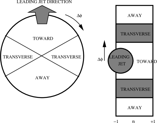
Figure 1: ‘Toward’, ‘away’ and ‘transverse’ regions defined with respect to the azimuthal direction of the leading charged jet.

As shown in fig. 1, three areas in the $\eta-\phi$ space are defined with respect to the azimuthal direction of the leading charged jet. $\eta$ is restricted to be between $-1$ and $+1$, and the three regions are defined according to the azimuthal angle. The ‘toward’ direction is centred around the leading jet direction and is within $\pi/3$ radians from the jet direction. The ‘transverse’ direction is between $\pi/3$ and $2\pi/3$ radians away from the jet direction. The ‘away’ direction is more than $2\pi/3$ radians away from the jet direction. The three regions have equal area of $4\pi/3$ in the $\eta-\phi$ space.

The quantities considered in ref. [1], that characterize the underlying hadronic activity, are the average scalar sum $p_{T}^{\mathrm{sum}}$ of $p_{T}$ of charged particles with $p_{T}$ greater than 0.5 GeV, and the charged particle multiplicity $N_{\mathrm{chrg}}$, in the three regions described above. These quantities were plotted against the $p_{T}$ of the leading charged jet.

Out of the three regions, the region that is most sensitive to the underlying event is the transverse direction.

2.5 Current status of HERWIG based simulation

Figure 2: Comparison of ‘transverse’ hadronic activity, in terms of $N_{\mathrm{chrg}}$ (left) and $p_{T}^{\mathrm{sum}}$ (right), in various HERWIG-based simulations, taken from ref. [5]. HERWIG+‘Eikonal’ model (solid line), HERWIG+‘Underlying Event’ model (solid dashed), HERWIG+‘Multiparton Hard’ model (dotted). Experimental data is shown with error-bars.

Fig. 2, taken from ref. [5], shows the current status of the fits to the Tevatron data using HERWIG-based simulations.

The default HERWIG curve is very much below the experimental numbers, but this is subject to the tuning of parameters. The numbers shown in ref. [1] are in better agreement, although still being lower than the experimental result.

The ‘multi-parton hard’ model is the result of simulation using JIMMY [4]. The simulation is based on the overlap-function approach. The plot shown has $p_{T}^{\mathrm{min}}=3$ GeV. The level of hadronic activity is not sufficiently high, and better agreement with data is obtained when the inclusive cross section is boosted by lowering $p_{T}^{\mathrm{min}}$ to 2 GeV.

The ‘eikonal’ model is an extension of the JIMMY approach where the $gg\to gg$ scatters below $p_{T}^{\mathrm{min}}=3$ GeV are also generated by modelling the inclusive cross section as an exponential function of $p_{T}^{2}$. The gluon structure function is assumed to have a $\propto 1/x$ behaviour. The dependence on $p_{T}^{\mathrm{min}}$ is, according to their claim [5], weakened, but is nevertheless present. The numbers drop considerably when $p_{T}^{\mathrm{min}}$ is lowered to 2 GeV. In our opinion, this is simply because the inclusive cross section in reality behaves more as a power, $\sim p_{T}^{-3}$, than an exponential.

The ‘eikonal’ model fits the data best out of the three approaches. This is because there is not sufficient hadronic activity in the other two approaches and this model adds a large amount of ‘soft’ activity from below $p_{T}^{\mathrm{min}}$.

As far as the shape of the fit is concerned, there are two remaining problems that are not rectified, which are:

1. When $p_{T}^{\mathrm{min}}$ is adjusted to fit $N_{\mathrm{chrg}}$, there is insufficient $p_{T}^{\mathrm{sum}}$. In other words, the charged particles in the underlying event carry too little $p_{T}$.

2. The slope at low $p_{T}$ is too steep, i.e., there is too much activity when $p_{T}$ of the leading jet is small. In other words, the underlying event is too uniform.

The above two points seem to indicate two things.

First, the description of fragmentation in low $p_{T}$ scatters is not adequate.

Second, the excessive uniformness of the simulated underlying event suggests that the idea of employing the cross section below $p_{T}^{\mathrm{min}}$ might actually not reflect the true nature of the underlying event. This same point applies to the model intrinsic to HERWIG, which also seems to have too much activity implicitly assigned to low $p_{T}$ physics.

There is a finding in ref. [2] that, in the PYTHIA framework, one needs a double-Gaussian overlap function with a ‘hard core’ in order to fit the data. We note that this is possibly another phenomenological indication of the non-uniformity of the observed underlying event.

One possibility for large $p_{T}^{\mathrm{min}}$ is that it should be kept high at the scale of the Regge-perturbative ‘transition’, or where colour singlet interactions become more dominant. This would seem to be in agreement with the observation made earlier that $\sigma_{\mathrm{eff}}$ is much smaller in reality than is supposed in ref. [5]. If $\sigma_{\mathrm{eff}}$ is smaller, larger activity can be obtained for smaller $\sigma^{\mathrm{inc}}$.

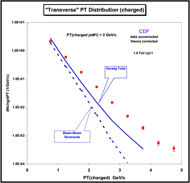
Figure 3: Transverse momentum distribution of charged particles ($p_{T}>0.5$ GeV,$|\eta|<1$) in the ‘transverse’ region, for leading jet $p_{T}>2$ GeV. Experimental data is compared against the HERWIG prediction. The dashed curve shows the underlying event contribution. Figure taken from ref. [1].

In ref. [1], in addition to the measurement of $N_{\mathrm{chrg}}$ and $p_{T}^{\mathrm{sum}}$, there is also the measurement of the $p_{T}$ of individual charged tracks in the ‘transverse’ region. This is reproduced in fig. 3 and we see that the model intrinsic in HERWIG produces too many soft tracks. In ref. [1], a study was made using the other generators, and the result was that PYTHIA gives slightly better description of the $p_{T}$ distribution although the slope is still too steep.

One can easily confirm that the excessive softness of the charged tracks shown in fig. 3 is quantitatively consistent with our earlier observation that when $p_{T}^{\mathrm{min}}$ is adjusted to fit $N_{\mathrm{chrg}}$, there is insufficient $p_{T}^{\mathrm{sum}}$.

2.6 ‘Perturbative’ nature of the underlying event

We remarked above that one of the reasons for the discrepancies between theory and experiment may be that the scatters take place at larger $p_{T}$ than is usually supposed, with $p_{T}^{\mathrm{min}}$ being determined by the Regge characteristic scale. If so, one would expect that, to a good approximation, each scatter may be calculated using perturbation theory.

To justify this claim in terms of the underlying theory, one needs to argue that the scatters from the Regge region do not contribute to the underlying event. This may be done in two steps by first showing that the Regge inclusive cross section may be suppressed and then arguing that the fragmentation in this region contributes less hadronic activity.

In the perturbative region, for $p_{T}^{\mathrm{min}}$ reasonably small, $\mathcal{O}(>2)$ GeV, the dependence of the inclusive cross section on $p_{T}^{\mathrm{min}}$ is found to be roughly $\sigma^{\mathrm{inc}}\sim(1/p_{T}^{\mathrm{min}})^{\sim 3}$. We have found numerically that the hadronic activity in default HERWIG also goes as $(1/p_{T}^{\mathrm{min}})^{2\sim 3}$.

On the other hand, if the low $p_{T}$ scattering cross section is determined by Regge dynamics, one may expect a form of the differential cross section that goes as $d\sigma^{\mathrm{inc}}/dp_{T}^{2}\sim p_{T}^{2\epsilon}$, with $\epsilon$ being a suitable Pomeron intercept. Hence the low $p_{T}$ cross section is suppressed compared with the perturbative behaviour. We do not yet specify the nature of this Pomeron here, but our analysis is inspired by the hard Pomeron picture of refs. [14, 15].

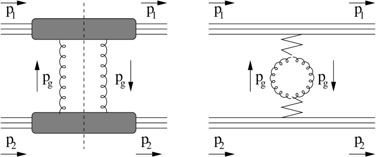
Figure 4: The low $p_{T}$ colour-octet exchange cross section (left) can be represented as the imaginary part of the bubble insertion in the Pomeron exchange diagram (right).

One possible picture which produces this $p_{T}$ dependence is illustrated in fig. 4. We represent the ‘resolved’ cross section by the colour-octet gluon exchange cross section, and this is written as the imaginary part of the bubble insertion in the Pomeron exchange diagram.

We write the helicity and colour conserving gluon–proton amplitude at zero momentum transfer as:

$$\mathcal{A}(g^{A}_{\lambda_{g}}p_{\lambda_{p}}\to g^{A}_{\lambda_{g}}p_{\lambda_{p}})\Big{|}_{t=0}=i\beta_{gp}\left(\frac{M_{pg}^{2}}{s_{0}}\right)^{1+\epsilon}.$$ (22)

We have defined $\beta_{gp}$ as a dimensionless quantity. It is proportional to the product of the dimension–$(-1)$ Pomeron couplings to the gluon and to the proton. $\epsilon$ is the Pomeron intercept. $s_{0}$ is the Regge characteristic scale and is about 4 GeV² [14]. As this is an overall factor only, the normalization may as well be traded between $\beta_{gp}$ and $s_{0}$.

In ref. [16], it is argued that the Pomeron coupling to off-shell partons cannot be considered to be point-like and that one should introduce a form factor with scale $\mathcal{O}(1$ GeV). Thus the above formulation is valid only below this scale. Above this scale, the form factor should suppress the cross section in such a way to reproduce the perturbative result $\sigma^{\mathrm{inc}}\sim(1/p_{T}^{\mathrm{min}})^{\sim 3}$. This picture is in accord with the recent studies [15].

The whole proton–proton amplitude at zero momentum transfer then follows:

$$\mathcal{A}_{\mathrm{bubble}}(p_{\lambda_{1}}p_{\lambda_{2}}\to p_{\lambda_{1}}p_{\lambda_{2}})\Big{|}_{t=0}=2i\beta_{gp}^{2}(N_{C}^{2}-1)\int\frac{d^{4}p_{g}}{(2\pi)^{4}p_{g}^{4}}\left(\frac{M_{1g}^{2}}{s_{0}}\right)^{1+\epsilon}\left(\frac{M_{2g}^{2}}{s_{0}}\right)^{1+\epsilon}.$$ (23)

The factor 2 in the front is for the two transverse polarizations of the gluon. The Pomeron coupling is thought to conserve helicity. We have added the subscript to $\mathcal{A}_{\mathrm{bubble}}$ to emphasize the point that we are not calculating the total elastic and inelastic cross section but only the ‘resolved’ cross section, here being identified with the colour octet transfer contribution. The $pp\to X$ cross section is then calculated by the optical theorem:

$$\sigma_{\mathrm{res}}^{\mathrm{inc}}(pp\to X)=\frac{1}{s_{\mathrm{CM}}}\mathrm{Im}\mathcal{A}_{\mathrm{bubble}}(pp\to pp)\Big{|}_{t=0}.$$ (24)

Neglecting the proton mass, let us define the four-momenta as follows:

$$p_{1} = \frac{\sqrt{s_{\mathrm{CM}}}}{2}\left(1,0,0,1\right),$$

$$p_{2} = \frac{\sqrt{s_{\mathrm{CM}}}}{2}\left(1,0,0,-1\right),$$

$$p_{g} = \left(E,\mathbf{p}_{T},-p_{z}\right).$$ (25)

$p_{z}$ is positive definite and satisfies $p_{z}>|E|$.

We express the phase space in terms of $\mathbf{p}_{T}$ and rapidity as:

$$d^{4}p_{g}=\frac{1}{2}d^{2}\mathbf{p}_{T}dt_{g}dy=\frac{\pi}{2}d\mathbf{p}_{T}^{2}dt_{g}dy.$$ (26)

Here $t_{g}=p_{g}^{2}$. We added the subscript to avoid confusion with the overall momentum transfer in the amplitude, which is zero. We define rapidity as:

$$y=\frac{1}{2}\ln\frac{p_{z}+E}{p_{z}-E}.$$ (27)

The two invariant masses squared in eqn. (23) are given by:

$$M_{1g}^{2} = p_{g}^{2}+\sqrt{s_{\mathrm{CM}}}(p_{z}+E)=t_{g}+e^{y}\sqrt{s_{\mathrm{CM}}(-t_{g}-\mathbf{p}_{T}^{2})},$$

$$M_{2g}^{2} = p_{g}^{2}+\sqrt{s_{\mathrm{CM}}}(p_{z}-E)=t_{g}+e^{-y}\sqrt{s_{\mathrm{CM}}(-t_{g}-\mathbf{p}_{T}^{2})}.$$ (28)

As $M_{1g}^{2},M_{2g}^{2}>0$, we have the inequalities:

$$|y| < \ln\left(\frac{\sqrt{s_{\mathrm{CM}}(-t_{g}-\mathbf{p}_{T}^{2})}}{-t_{g}}\right),$$

$$0<\mathbf{p}_{T}^{2} < -t_{g}-t_{g}^{2}/s_{\mathrm{CM}}.$$ (29)

The gluon virtuality terms $t_{g}$ in eqn. (28) are small and so let us neglect them. This is admissible as the cross section is small-$x$ dominated in the structure function language. The $y$ integration yields a logarithm which is approximately $\ln(s_{\mathrm{CM}}/s_{0})$. The remaining integration in eqn. (23), expressed in terms of $(d\sigma^{\mathrm{inc}}_{\mathrm{res}}/dt_{g})$, is merely:

$$\frac{d\sigma^{\mathrm{inc}}_{\mathrm{res}}}{dt_{g}}\approx\frac{\beta_{gp}^{2}(N_{C}^{2}-1)}{16\pi^{3}s_{0}t_{g}^{2}}\left(\frac{s_{\mathrm{CM}}}{s_{0}}\right)^{\epsilon}\ln\left(\frac{s_{\mathrm{CM}}}{s_{0}}\right)\int d|m_{T}^{2}|\left(\frac{|m_{T}^{2}|}{s_{0}}\right)^{1+\epsilon}.$$ (30)

The proton helicities have been averaged over. We have defined $m_{T}^{2}=t_{g}+\mathbf{p}_{T}^{2}$ which is negative definite from eqn. (29). The $m_{T}^{2}$ integration is of course trivial. Neglecting the small contribution from the lower limit of integration, we obtain:

$$\frac{d\sigma^{\mathrm{inc}}_{\mathrm{res}}}{dt_{g}}\approx\frac{\beta_{gp}^{2}(N_{C}^{2}-1)}{16\pi^{3}s_{0}^{2}(2+\epsilon)}\left(\frac{s_{\mathrm{CM}}}{s_{0}}\right)^{\epsilon}\left(\frac{-t_{g}}{s_{0}}\right)^{\epsilon}\ln\left(\frac{s_{\mathrm{CM}}}{s_{0}}\right).$$ (31)

Thus the cross section has a $(-t_{g})^{\epsilon}$ behaviour and falls to zero at zero gluon virtuality rather than increasing indefinitely. $(-t_{g})$ can be loosely exchanged with $\mathbf{p}_{T}^{2}$ and hence we have demonstrated the power behaviour of the low $p_{T}$ cross section claimed earlier.

It is possible to interpret the above discussion in terms of the hard Pomeron picture of ref. [15], with $\epsilon\approx 0.4$. This provides a means of fixing the normalization of eqn. (31), by using the gluon structure function.

Let us consider the first diagram of fig. 4 but with the upper proton replaced by the gluon. We write the $gg\to gg$ amplitude at zero momentum transfer, averaged over the first gluon colour and helicity, as:

$$\mathcal{A}(gg^{A}_{\lambda_{g}}\to gg^{A}_{\lambda_{g}})\Big{|}_{t=0}=iM^{2}_{gg}\widehat{\sigma}_{gg}(M^{2}_{gg}).$$ (32)

The whole amplitude is then:

$$\mathcal{A}(gp_{\lambda_{p}}\to gp_{\lambda_{p}})\Big{|}_{t=0} = 2i\beta_{gp}(N_{C}^{2}-1)\int\frac{d^{4}p_{g}}{(2\pi)^{4}p_{g}^{4}}M_{1g}^{2}\widehat{\sigma}_{gg}(M^{2}_{1g})\left(\frac{M_{2g}^{2}}{s_{0}}\right)^{1+\epsilon}$$ (33)

$$= i\frac{\beta_{gp}(N_{C}^{2}-1)}{16\pi^{3}}\int dt_{g}d\mathbf{p}_{T}^{2}dyM_{1g}^{2}\widehat{\sigma}_{gg}(M^{2}_{1g})\left(\frac{M_{2g}^{2}}{s_{0}}\right)^{1+\epsilon}.$$

We are interested in the structure function $f_{g}(x,Q^{2})=(\partial\sigma/\partial x)/\widehat{\sigma}$. We define $x=(p_{Z}+E)/\sqrt{s_{\mathrm{CM}}}$ and omit $t_{g}$ in eqn. (28) as before, to obtain:

$$f_{g}(x,Q^{2})\approx\frac{\beta_{gp}(N_{C}^{2}-1)}{16\pi^{3}}\int_{t_{g}=0}^{t_{g}=Q^{2}}\frac{dt_{g}}{t_{g}^{2}}d|m_{T}^{2}|\left(\frac{-m_{T}^{2}}{s_{0}x}\right)^{1+\epsilon}.$$ (34)

Hence, neglecting the lower limit of $m_{T}^{2}$ integration as before, we obtain:

$$f_{g}(x,Q^{2})\approx\frac{\beta_{gp}(N_{C}^{2}-1)}{16\pi^{3}(1+\epsilon)(2+\epsilon)}\left(\frac{Q^{2}}{s_{0}x}\right)^{1+\epsilon}.$$ (35)

We may compare this with the form given in ref. [15]:

$$xg(x,Q^{2})\sim 0.95(Q^{2})^{1+\epsilon_{0}}(1+Q^{2}/0.5)^{-1-\epsilon_{0}/2}x^{-\epsilon_{0}}.$$ (36)

The units for $Q^{2}$ are in GeV². This form is claimed to be valid in the range $5<Q^{2}<500$ GeV². $\epsilon_{0}$ is the hard Pomeron intercept which, in our notation, is $\epsilon\approx 0.4$. Because of the presence of the extra denominator factor $(1+Q^{2}/0.5)^{-1-\epsilon_{0}/2}$, the normalization is ambiguous. For instance, if we extend their claimed range of applicability to the limit of very low $Q^{2}$ and match the two expressions at $Q^{2}=0$, we obtain a cross section which is unreasonably large. Let us match the two equations at the lowest end, $Q^{2}=5$ GeV², of the range of validity of eqn. (36). We obtain:

$$\frac{\beta_{gp}(N_{C}^{2}-1)}{16\pi^{3}(1+\epsilon)(2+\epsilon)}\sim 0.05$$ (37)

At $\sqrt{s}_{\mathrm{CM}}=1.8$ TeV, we then obtain from eqn. (31):

$$\frac{d\sigma^{\mathrm{inc}}_{\mathrm{res}}}{dt_{g}}\approx 30\ \mathrm{mb\ GeV}^{-2}\left(\frac{-t_{g}}{s_{0}}\right)^{\epsilon}.$$ (38)

As stated above, there is ambiguity in the normalization due to our lack of knowledge about the structure function at very low $Q^{2}$.

2.7 Fragmentation in low $p_{T}$ scatters

In addition to the Regge suppression of low $p_{T}$ scattering rate, we note that fragmentation may also be affected by Regge dynamics.

One characteristic behaviour is Reggeization. Partons that are emitted in the perturbative phase are coloured objects with colour partners, but in the Regge phase, they may become, in some sense, colour singlet. If this is the case, large rapidity gaps would be formed per scatter and hence the contribution to the underlying event would be reduced.

This effect is difficult to quantify, but since the leading effect is to suppress the low $p_{T}$ contribution, this provides another justification for neglecting it.

In ref. [11], we proposed that the splitting of large clusters in the cluster-hadronization model [12] of HERWIG can be connected to a modified QCD coupling that governs those emissions which are considered unresolved in the parton-shower phase. ‘Clusters’ are colour-singlet quark-antiquark units which result from the parton shower process followed by a forced $g\to q\bar{q}$ splitting. In HERWIG, they subsequently decay isotropically into hadrons according to the phase space weight.

The effect of this modification is not particularly large for processes occuring at large hard-process scale, but it is potentially significant for soft processes such as the underlying event. Therefore the study of the underlying event, in particular relatively inclusive quantities such as the $p_{T}$ distribution of charged particles shown in fig. 3, could provide a testing ground for models of hadronization.

One possibility that follows from the modified picture of hadronization is that because of the reduced phase space for parton emission in soft scatters, the resulting cluster size is typically larger than in the high $p_{T}$ processes. This is discussed in the next section, together with the possibility that this leads to different individual hadron yields.

3 Simulation and discussions

Fitting the experimental data with the simulation tools involves, in general, not a small number of tunable parameters. However, they are reducible to three components. First, the ‘effective cross section’ $\sigma_{\mathrm{eff}}$. Second, the inclusive cross section controlled by $p_{T}^{\mathrm{min}}$. Third, the distribution of the number of scatters controlled by the overlap function. Normally $\sigma_{\mathrm{eff}}$ is not an explicitly tunable parameter, so that one adjusts $p_{T}^{\mathrm{min}}$ to adjust the amount of hadronic activity. The distribution of the number of scatters then affects how much the multiple-scattering contribution fluctuates. In addition, one sometimes makes the cut-off at $p_{T}^{\mathrm{min}}$ smooth, and this also affects the shape of distributions.

We now abandon the overlap function and adopt a naive Poisson distribution. We hence have only one parameter, $p_{T}^{\mathrm{min}}$, that can be tuned to fit the amount of hadronic activity, and have an environment to study the fragmentation scheme dependence.

Although $p_{T}^{\mathrm{min}}$ is a tunable parameter, we should not set it too far from the onset of Regge physics. A reasonable value may be in the range $1-5$ GeV and so let us adopt 3 GeV for now. For $\sigma_{\mathrm{eff}}$, we adopt the measured value of 14.5 mb. We carry out the simulation simply by generating a number of QCD $(2\to 2)$ scatters on top of one another, without considering the constraint from the conservation of energy.

The experimental data is uncorrected and the theoretical numbers are corrected by removing, on average, 8% of the charged tracks.

Figure 5: Comparison of ‘transverse’ hadronic activity, in terms of $N_{\mathrm{chrg}}$ (above) and $p_{T}^{\mathrm{sum}}$ (below). Simulation at $p_{T}^{\mathrm{min}}=3$ GeV and $\sigma_{\mathrm{eff}}=14.5$ mb. The two hadronization schemes are explained in the text. Experimental data is shown with error-bars. Simulation sample size is one million events. Error-bars are not shown.

In fig. 5, we show the result of a simple simulation using HERWIG. The inclusive cross section is found to be about 27 mb so that about two scatters take place per event on average. With this value of $p_{T}^{\mathrm{min}}$, the normalization is found to match that of experimental data. We note that in ref. [5], $\sigma_{\mathrm{eff}}$ is about 60 mb but the inclusive cross section is larger and hence the average number of scatters per event is 2.4, not too dissimilar to the case studied here.

Two hadronization schemes are used. The first is the default cluster hadronization scheme of HERWIG. The second is the scheme proposed in ref. [11] which uses a Gaussian approximation for low energy $\alpha_{S}$ to describe the splitting of large clusters.

The normalization is smaller for the modified cluster splitting procedure based on the low-energy Gaussian $\alpha_{S}$. This is because when very large clusters are split, the modified procedure results in lighter daughter clusters and hence smaller multiplicity. We note that, for the same reason, the $p_{T}^{\mathrm{min}}$ dependence of the underlying hadronic activity is milder in this approach. This is welcome as it reduces the theoretical uncertainty due to $p_{T}^{\mathrm{min}}$.

The two discrepancies with experimental data mentioned in sec. 2 are still present to some extent, though the slope for low values of leading-jet $p_{T}$ is now in better agreement with experimental data. The remaining problem is that the tracks are still too soft.

Figure 6: Transverse momentum distribution of charged particles ($p_{T}>0.5$ GeV,$|\eta|<1$) in the ‘transverse’ region, for leading jet $p_{T}>2$ GeV. Experimental data is compared against the HERWIG prediction for the two hadronization schemes.

This last point is appreciated in a more quantitative fashion by considering the $p_{T}$ distribution of charged tracks in the transverse region, as shown in fig. 6.

There is better agreement between experimental data and simulation than in fig. 3, but some discrepancy still remains. The difference between the two hadronization schemes is small. The most visible difference is for the point at $p_{T}$ between 0.5 and 1 GeV, where the modified hadronization scheme results in fewer tracks, in better agreement with experimental data.

One possibility, as to the reason why the $p_{T}$ distribution of charged tracks is too soft even with large $p_{T}^{\mathrm{min}}$, has to do with the cluster splitting process. We proposed in ref. [11] that the splitting of large clusters is due to the parton emission that is considered unresolved in the usual parton-shower phase. If so, and considering that the scatters take place mostly at very low $p_{T}$, the typical size of clusters from scatters at low $p_{T}$ is expected to be larger due to the lack of phase space for parton emission.

Let us consider the cascade splitting of a cluster with mass $M_{\mathrm{init}}$. From ref. [11], for a cluster splitting process $0\to 12$ by unresolved parton emission at $p_{T}^{2}=Q^{2}$ we have:

$$Q^{2}=\frac{M_{1}^{2}M_{2}^{2}}{M_{0}^{2}},$$ (39)

and the number of splittings is given by:

$$\left<\#_{\mathrm{split}}\right>\sim I_{0}\log\frac{M_{\mathrm{init}}^{2}}{\left<Q^{2}\right>}.$$ (40)

Here $I_{0}$ is $C_{F}/\pi$ times the integral of low energy $\alpha_{S}$, and is found to be about 0.5. Combining the above two equations and considering cascade decay with final cluster masses $M_{\mathrm{final}}$, we obtain:

$$\left<\log\frac{M_{\mathrm{final}}^{2}}{Q^{2}}\right>=\frac{1}{I_{0}(1+1/\#_{\mathrm{split}})}.$$ (41)

In high $p_{T}$ processes, clusters that are formed before the cluster-splitting process have relatively low mass, with some large clusters having masses extending up to $\mathcal{O}$(10 GeV). In this case, the right hand side of eqn. (41) is about 1.5 for $\left<Q\right>\approx 0.75$ GeV. Hence we obtain $\left<M_{\mathrm{final}}\right>\approx 1.5$ GeV. On the other hand, in the large $M_{\mathrm{init}}$ limit, in other words $\#_{\mathrm{split}}\to\infty$, we obtain $\left<M_{\mathrm{final}}\right>\to 2$ GeV.

One simple way of modifying the typical cluster mass as a means to study this aspect of hadronization dynamics is to change the HERWIG parameter CLMAX, which is the maximum allowed cluster mass. This is imposed even in the case of the modified algorithm. Clusters with mass greater than CLMAX are split. We modify this, somewhat arbitrarily, from the default value of 3.35 GeV to 5 GeV. We adopt the low-energy $\alpha_{S}$ prescription for splitting clusters, as otherwise there is no incentive for modifying CLMAX.

Figure 7: Transverse momentum distribution of charged particles ($p_{T}>0.5$ GeV,$|\eta|<1$) in the ‘transverse’ region, for leading jet $p_{T}>2$ GeV. Experimental data is compared against the HERWIG prediction for the modified hadronization scheme with CLMAX set to 5 GeV.

The result, for the $p_{T}$ distribution of charged tracks, is shown in fig. 7, and is in very good agreement with CDF data.

Figure 8: Comparison of ‘transverse’ hadronic activity, in terms of $N_{\mathrm{chrg}}$ (above) and $p_{T}^{\mathrm{sum}}$ (below). Simulation at with CLMAX set to 5 GeV. Experimental data is shown with error-bars. Simulation sample size is ten million events. Error-bars are not shown.

The leading-jet $p_{T}$ dependence of the transverse hadronic activity, shown in fig. 8, also shows good agreement with data. In addition to the improved $p_{T}$ per charged track ratio, there is also improvement to the shape of the low leading-jet $p_{T}$ region.

The remaining difference may be due either to our incomplete description of hadronization or to the inaccurate distribution of the number of scatters. We have tested lowering $p_{T}^{\mathrm{min}}$ to 2.5 GeV and found that this results in too many soft tracks in fig. 7 so we believe that the wrong choice of $p_{T}^{\mathrm{min}}$ alone is not a likely possibility to explain the imperfect fit.

If the above speculations concerning the fragmentation in low $p_{T}$ scatters are correct, one would expect that the identified particle yields may be different. With enhanced cluster mass, there is more phase space for decay into heavier hadrons, for instance baryons, and hence we would expect increased baryon–meson ratio. This could be confirmed by measuring the proton–charged pion ratio $R_{p/\pi}$.

hadronization scheme	$N_{p,\overline{p}}$	$N_{\pi^{\pm}}$	$R_{p/\pi}$
HERWIG default	3748	18056	$0.208\pm 0.004$
Gaussian $\alpha_{S}$	2698	15032	$0.179\pm 0.004$
Large clusters	4334	14474	$0.299\pm 0.005$

Table 1: The proton to charged pion ratio, for tracks with $|\eta|<1$ and $p_{T}>0.5$ GeV, in the three hadronization schemes adopted in this study. Sample size is 10000 scatters. $p_{T}^{\mathrm{min}}=3$ GeV. The errors quoted are due to the Monte Carlo statistics only.

A simple simulation with a small statistics of 10000 scatters, sampling particles with $p_{T}>0.5$ GeV and $|\eta|<1$ only, yields the numbers shown in tab. 1. We see that in the case with CLMAX set to 5 GeV, there is about 50% increase in the proton yield as compared to the case with the default CLMAX of 3.35 GeV.

We note that even the unmodified case leads to substantially increased yield for protons compared with yields in high $p_{T}$ collision. For instance, the numbers from LEP at the $Z^{0}$ pole gives $R_{p/\pi}\approx 1/17$ [17].

We should say that some caution is needed as regards the numbers, as the identified particle yield for baryons is a poorly described quantity in HERWIG. Hence although the above argument does indicate that the proton yield is substantially enhanced in the underlying event, the exact numbers for the yield should not be trusted.

We propose the measurement of $R_{p/\pi}$, and other hadron yields, in the ‘toward’ and ‘transverse’ regions as a function of the leading jet $p_{T}$ as a way to understand the fragmentation properties of low $p_{T}$ scatters.

4 Conclusions and outlook

Conclusions

We studied the underlying event in the multiple-scattering picture at Tevatron.

We started by noting some deficiencies of the current theoretical description of the underlying event. We noted the possibility that the scatters affecting the underlying event take place at above the Regge-dominated regime and are therefore to a good approximation calculable using perturbation theory. We also noted that the description of fragmentation in low $p_{T}$ scatters needs to be improved.

We carried out our simulation on HERWIG using a naive Poisson distribution for the number of scatters, choosing $p_{T}^{\mathrm{min}}=3$ GeV and $\sigma_{\mathrm{eff}}=14.5$ mb, and found that by modifying the hadronization algorithm as suggested in our previous study and by adopting a larger maximum cluster size parameter CLMAX, a good agreement with data is obtained.

If our picture is correct, one would expect an enhancement in the baryon yield in the underlying event. We proposed that a measurement is made of this effect by measuring the proton-to-pion ratio as a function of the leading jet $p_{T}$. A confirmation of this effect, or otherwise, could shed light both on the nature of the underlying event and on the nature of the dynamics of hadronization.

Outlook

A possible future improvement to our study may come from a better understanding of the distribution of the number of scatters per event, or in other words the mechanism of unitarization of scattering probabilities. We desire further experimental study, in particular the measurement of $\sigma_{\mathrm{eff}}$ on distinct experimental platforms, for instance in resolved $\gamma p$ and $\gamma\gamma$ collisions, and at different $\sqrt{s_{\mathrm{CM}}}$. The large $\sqrt{s_{\mathrm{CM}}}$ available at LHC will give rise to larger mean number of scatters per event. This will be significant aid to the study of the distribution of the number of scatters.

Additionally to the results presented herein, we have made a small-statistics calculation for the underlying event at LHC using the same $\sigma_{\mathrm{eff}}$ and $p_{T}^{\mathrm{min}}$. The flattening-off of the transverse hadronic activity occurs at larger trigger-jet $p_{T}$. For sufficiently large $p_{T}$, both $N_{\mathrm{chrg}}$ and $p_{T}^{\mathrm{sum}}$ are found to be about 5 times greater than at Tevatron. This coincides with the latest results using PYTHIA [6, 18]. On the other hand, the inclusive cross section at LHC is 220 mb according to HERWIG, which is about 8 times that at Tevatron. The greater part of the difference is presumably due to the difference in the allowed rapidity range, i.e., there are more forward scatters at LHC than at Tevatron. We have made simple phase-space estimations to confirm this point.

The HERWIG sub-version 6.505 has appeared recently. One of the major ingredients in this release is an interface to JIMMY. It is a simple matter to modify this HERWIG–JIMMY package to generate scatters according to a Poisson distribution as in our approach. This merely involves the substitution of the overlap function by a step function, i.e., $A(b^{2})=\Theta(\sigma_{\mathrm{eff}}-\pi b^{2})/\sigma_{\mathrm{eff}}$. We have made some calculations by adopting this, and the results are consistent with those presented in this study.