A General analysis of the lepton polarizations in $B_{s}\rightarrow\gamma\,\ell^{+}\ell^{-}$ decays

We present a general analysis of the lepton polarizations in the rare $B_{s}\rightarrow\gamma\,\ell^{+}\ell^{-}$ decays by using the most general model independent form of the effective Hamiltonian. The sensitivity of the longitudinal, transverse and normal polarizations of final state leptons, as well as lepton-antilepton combined asymmetries, on the new Wilson coefficients are investigated. It has been shown that all these physical observables are very sensitive to the existence of new physics beyond the standard model and their experimental measurements can give valuable information about it.

PACS number(s): 12.60.Fr, 13.20.He

1 Introduction

It has been already pointed out many times before [1] that the rare B meson decays, as being flavor changing neutral current (FCNC) processes, are sensitive to the structure of the standard model (SM), and its possible extensions. Therefore, these decays may serve as an important tool to investigate the new physics prior to any possible experimental clue about it. The experimental situation concerning B physics is promising too. In addition to several experiments running successfully like the BELLE experiment at KEK and the BaBar at SLAC, new facilities will also start to explore B physics in a near future, like the LHC-B experiment at CERN and BTeV at FERMILAB.

Among the rare B-meson decays, the semileptonic $B_{s}\rightarrow\gamma\,\ell^{+}\ell^{-}$ $(\ell=e,\mu,\tau)$ decays are especially interesting due to their relative cleanliness and sensitivity to new physics. $B_{s}\rightarrow\gamma\,\ell^{+}\ell^{-}$decay is induced by $B\rightarrow\,\ell^{+}\ell^{-}$ one, which can be in principle serve as a useful process to determine the fundamental parameters of the SM since the only non-perturbative quantity in its theoretical calculation is the decay constant $f_{B_{s}}$, which is reliably known. However, in the SM, matrix element of $B\rightarrow\,\ell^{+}\ell^{-}$ decay is proportional to the lepton mass and therefore corresponding branching ratio will be helicity suppressed. Although $\ell=\tau$ channel is free from this suppression, its experimental observation is quite difficult due to low efficiency. In this connection, it has been pointed out [2]-[11] that the radiative leptonic $B^{+}\rightarrow\ell^{+}\,\nu_{\ell}\,\gamma$ $(\ell=e,\mu)$ decays have larger branching ratios than purely leptonic modes. It has been shown [7, 12] that similar enhancements take place also in the radiative decay $B_{s}\rightarrow\gamma\,\ell^{+}\ell^{-}$, in which the photon emitted from any of the charged lines in addition to the lepton pair makes it possible to overcome the helicity suppression. For that reason, the investigation of the $B_{s}\rightarrow\gamma\,\ell^{+}\ell^{-}$decays becomes interesting.

As an exclusive process, the theoretical calculation of $B_{s}\rightarrow\gamma\,\ell^{+}\ell^{-}$decay requires the additional knowledge about the decay form factors. These are the matrix elements of the effective Hamiltonian between the initial B and final photon states, when a photon is released from the initial quark lines, which give rise to the so called ”structure dependent” (SD) contributions to the amplitude, and between the B and the vacuum states for the ”internal Bremsstrahlung” (IB) part, which arises when a photon is radiated from final leptons. Finding these hadronic transition matrix elements is related to the nonperturbative sector of the QCD and should be calculated by means of a nonperturbative approach. Thus, their theoretical calculation yields the main uncertainty in the prediction of the exclusive rare decays. The form factors for B decays into $\gamma$ and a vacuum state have been calculated in the framework of light-cone QCD sum rules in [3, 7] and in the framework of the light front quark model in [13]. In addition, it has been proposed a model in [14] for the $B\rightarrow\gamma$ form factors which obey all the restrictions obtained from the gauge invariance combined with the large energy effective theory.

Various kinematical distributions of the $B_{s}\rightarrow\gamma\,\ell^{+}\ell^{-}$decays have been studied in many earlier works. The analiysis in the framework of the SM can be found in [7, 8, 12, 13]. The new physics effects in these decays have been studied in some models, like minimal supersymmetric Standard model (MSSM) [15]-[18] and the two Higgs doublet model [19]-[22], and shown that different observables, like branching ratio, forward-backward asymmetry, etc., are very sensitive to the physics beyond the SM. In $B_{s}\rightarrow\gamma\,\ell^{+}\ell^{-}$decay, in addition to the branching ratio and lepton pair forward-backward asymmetry, it is possible to study some other experimentally observable quantities associated with the final state leptons and photon, such as the photon and lepton polarization asymmetries. Along this line, the polarization asymmetries of the final state lepton in $B_{s}\rightarrow\gamma\ell^{+}\ell^{-}$ decays have been studied in MSSM in [18] and concluded that they can be very useful for accurate determination of various Wilson coefficients. In addition, in a recent work [23] we have been considered the effects of polarized photon in the $B_{s}\rightarrow\gamma\,\ell^{+}\ell^{-}$decay and shown that its spectrum is sensitive to the new physics effects.

In this work, we will investigate the new physics effects in the lepton polarization asymmetries in the $B_{s}\rightarrow\gamma\,\ell^{+}\ell^{-}$decay. Final state leptons in the $B_{s}\rightarrow\gamma\,\ell^{+}\ell^{-}$decay can have longitudinal $P_{L}$, transverse $P_{T}$ and normal $P_{N}$ polarizations, where $P_{T}$ is the component of the polarization lying in the decay plane and $P_{N}$ is the one that is normal to the decay plane. Since these three components contain different combinations of Wilson coefficients and hence provide independent information they are thought to play important role in further investigations of the SM and its possible extensions. As for the new physics effects, in rare $B$ meson decays they can appear in two different ways: one way is through new contributions to the Wilson coefficients that is already present in the SM, and the other is through the new operators in the effective Hamiltonian which is absent in the SM. In this work we use a most general model independent effective Hamiltonian that combines both these approaches and contains the scalar and tensor type interactions as well as the vector types (see Eq.(2) below).

The paper is organized as follows: In Sec. 2, we first give the effective Hamiltonian for the quark level process $b\rightarrow s\ell^{+}\ell^{-}$ and the definitions of the form factors, and then introduce the corresponding matrix element. In Secs. 3 and 4, we present the analytical expressions of the various lepton polarization asymmetries and lepton-antilepton combined asymmetries, respectively. Sec. 5 is devoted to the numerical analysis and discussion of our results.

2 Effective Hamiltonian

For the radiative $B_{s}\rightarrow\gamma\,\ell^{+}\ell^{-}$decay, the basic quark level process is $b\rightarrow s\ell^{+}\ell^{-}$, which can be written in terms of twelve model independent four-Fermi interactions as follows [24]:

$${\cal H}_{eff} = \frac{\alpha\,G}{\sqrt{2}\,\pi}V_{ts}V_{tb}^{\ast}\Bigg{\{}C_{SL}\,\bar{s}i\sigma_{\mu\nu}\frac{q^{\nu}}{q^{2}}\,L\,b\,\bar{\ell}\gamma^{\mu}\ell+C_{BR}\,\bar{s}i\sigma_{\mu\nu}\frac{q^{\nu}}{q^{2}}\,R\,b\,\bar{\ell}\gamma^{\mu}\ell$$

$$+C_{LL}^{tot}\,\bar{s}_{L}\gamma_{\mu}b_{L}\,\bar{\ell}_{L}\gamma^{\mu}\ell_{L}+C_{LR}^{tot}\,\bar{s}_{L}\gamma_{\mu}b_{L}\,\bar{\ell}_{R}\gamma^{\mu}\ell_{R}+C_{RL}\,\bar{s}_{R}\gamma_{\mu}b_{R}\,\bar{\ell}_{L}\gamma^{\mu}\ell_{L}$$

$$+C_{RR}\,\bar{s}_{R}\gamma_{\mu}b_{R}\,\bar{\ell}_{R}\gamma^{\mu}\ell_{R}+C_{LRLR}\,\bar{s}_{L}b_{R}\,\bar{\ell}_{L}\ell_{R}+C_{RLLR}\,\bar{s}_{R}b_{L}\,\bar{\ell}_{L}\ell_{R}$$

$$+C_{LRRL}\,\bar{s}_{L}b_{R}\,\bar{\ell}_{R}\ell_{L}+C_{RLRL}\,\bar{s}_{R}b_{L}\,\bar{\ell}_{R}\ell_{L}+C_{T}\,\bar{s}\sigma_{\mu\nu}b\,\bar{\ell}\sigma^{\mu\nu}\ell$$

$$+iC_{TE}\,\epsilon^{\mu\nu\alpha\beta}\bar{s}\sigma_{\mu\nu}b\,\bar{\ell}\sigma_{\alpha\beta}\ell\Bigg{\}}~{},$$

where $L=(1-\gamma_{5})/2$ and $R=(1+\gamma_{5})/2$ are the chiral projection operators. In Eq. (2), $C_{X}$ are the coefficients of the four–Fermi interactions with $X=LL,LR,RL,RR$ describing vector, $X=LRLR,RLLR,LRRL,RLRL$ scalar and $X=T,TE$ tensor type interactions. We note that the coefficients $C_{SL}$ and $C_{BR}$ correspond to $-2m_{s}C_{7}^{eff}$ and $-2m_{b}C_{7}^{eff}$ in the SM, while $C_{LL}$ and $C_{LR}$ are in the form $C_{9}^{eff}-C_{10}$ and $C_{9}^{eff}+C_{10}$, respectively. Therefore, writing

$$C_{LL}^{tot} = C_{9}^{eff}-C_{10}+C_{LL}~{},$$

$$C_{LR}^{tot} = C_{9}^{eff}+C_{10}+C_{LR}~{},$$

we observe that $C_{LL}^{tot}$ and $C_{LR}^{tot}$ contain the contributions from the SM and also from the new physics.

Having established the general form of the effective Hamiltonian, the next step is to calculate the matrix element of the $B_{s}\rightarrow\gamma\,\ell^{+}\ell^{-}$ decay, which can be written as a sum of the SD and the IB parts:

$${\cal M}={\cal M}_{SD}+{\cal M}_{IB}.$$ (2)

Using the expressions [3, 7]

$$\left<\gamma(k)\left|\bar{s}\gamma_{\mu}(1\mp\gamma_{5})b\right|B(p_{B})\right> = \frac{e}{m_{B}^{2}}\Big{\{}\epsilon_{\mu\nu\lambda\sigma}\varepsilon^{\ast\nu}q^{\lambda}k^{\sigma}g(q^{2})$$ (3)

$$\pm i\,\Big{[}\varepsilon^{\ast\mu}(kq)-(\varepsilon^{\ast}q)k^{\mu}\Big{]}f(q^{2})\Big{\}}~{},$$

$$\left<\gamma(k)\left|\bar{s}\sigma_{\mu\nu}b\right|B(p_{B})\right> = \frac{e}{m_{B}^{2}}\epsilon_{\mu\nu\lambda\sigma}\Big{[}G\varepsilon^{\ast\lambda}k^{\sigma}+H\varepsilon^{\ast\lambda}q^{\sigma}+N(\varepsilon^{\ast}q)q^{\lambda}k^{\sigma}\Big{]}~{},$$ (4)

$$\left<\gamma(k)\left|\bar{s}(1\mp\gamma_{5})b\right|B(p_{B})\right> = 0~{},$$ (5)

$$\left<\gamma(k)\left|\bar{s}i\sigma_{\mu\nu}q^{\nu}b\right|B(p_{B})\right> = \frac{e}{m_{B}^{2}}i\,\epsilon_{\mu\nu\alpha\beta}q^{\nu}\varepsilon^{\alpha\ast}k^{\beta}G~{},$$ (6)

and

$$\left<\gamma(k)\left|\bar{s}i\sigma_{\mu\nu}q^{\nu}(1+\gamma_{5})b\right|B(p_{B})\right> = \frac{e}{m_{B}^{2}}\Big{\{}\epsilon_{\mu\alpha\beta\sigma}\,\varepsilon^{\alpha\ast}q^{\beta}k^{\sigma}g_{1}(q^{2})+i\,\Big{[}\varepsilon_{\mu}^{\ast}(qk)-(\varepsilon^{\ast}q)k_{\mu}\Big{]}f_{1}(q^{2})\Big{\}}~{},$$

the SD part of the amplitude can be written as

$${\cal M}_{SD} = \frac{\alpha G_{F}}{4\sqrt{2}\,\pi}V_{tb}V_{ts}^{*}\frac{e}{m_{B}^{2}}\,\Bigg{\{}\bar{\ell}\gamma^{\mu}(1-\gamma_{5})\ell\,\Big{[}A_{1}\epsilon_{\mu\nu\alpha\beta}\varepsilon^{\ast\nu}q^{\alpha}k^{\beta}+i\,A_{2}\Big{(}\varepsilon_{\mu}^{\ast}(kq)-(\varepsilon^{\ast}q)k_{\mu}\Big{)}\Big{]}$$

$$+ \bar{\ell}\gamma^{\mu}(1+\gamma_{5})\ell\,\Big{[}B_{1}\epsilon_{\mu\nu\alpha\beta}\varepsilon^{\ast\nu}q^{\alpha}k^{\beta}+i\,B_{2}\Big{(}\varepsilon_{\mu}^{\ast}(kq)-(\varepsilon^{\ast}q)k_{\mu}\Big{)}\Big{]}$$

$$+ i\,\epsilon_{\mu\nu\alpha\beta}\bar{\ell}\sigma^{\mu\nu}\ell\,\Big{[}G\varepsilon^{\ast\alpha}k^{\beta}+H\varepsilon^{\ast\alpha}q^{\beta}+N(\varepsilon^{\ast}q)q^{\alpha}k^{\beta}\Big{]}$$

$$+ i\,\bar{\ell}\sigma_{\mu\nu}\ell\,\Big{[}G_{1}(\varepsilon^{\ast\mu}k^{\nu}-\varepsilon^{\ast\nu}k^{\mu})+H_{1}(\varepsilon^{\ast\mu}q^{\nu}-\varepsilon^{\ast\nu}q^{\mu})+N_{1}(\varepsilon^{\ast}q)(q^{\mu}k^{\nu}-q^{\nu}k^{\mu})\Big{]}\Bigg{\}}~{},$$

where

$$A_{1} = \frac{1}{q^{2}}\Big{(}C_{BR}+C_{SL}\Big{)}g_{1}+\Big{(}C_{LL}^{tot}+C_{RL}\Big{)}g~{},$$

$$A_{2} = \frac{1}{q^{2}}\Big{(}C_{BR}-C_{SL}\Big{)}f_{1}+\Big{(}C_{LL}^{tot}-C_{RL}\Big{)}f~{},$$

$$B_{1} = \frac{1}{q^{2}}\Big{(}C_{BR}+C_{SL}\Big{)}g_{1}+\Big{(}C_{LR}^{tot}+C_{RR}\Big{)}g~{},$$

$$B_{2} = \frac{1}{q^{2}}\Big{(}C_{BR}-C_{SL}\Big{)}f_{1}+\Big{(}C_{LR}^{tot}-C_{RR}\Big{)}f~{},$$

$$G = 4C_{T}g_{1}~{}~{}~{},~{}~{}~{}N=-4C_{T}\frac{1}{q^{2}}(f_{1}+g_{1})~{},$$

$$H = N(qk)~{}~{}~{},~{}~{}~{}G_{1}=-8C_{TE}g_{1}~{},$$

$$N_{1} = 8C_{TE}\frac{1}{q^{2}}(f_{1}+g_{1})~{}~{}~{},~{}~{}~{}H_{1}=N_{1}(qk)~{}.$$

Here, $\varepsilon_{\mu}^{\ast}$ and $k_{\mu}$ are the four vector polarization and four momentum of the photon, respectively, $q$ is the momentum transfer, $p_{B}$ is the momentum of the $B$ meson, and $G,~{}H$ and $N$ have been expressed in terms of the form factors $g_{1}$ and $f_{1}$ by using Eqs. (4), (6) and (2).

When photon is radiated from the lepton line we get the the so-called ”internal Bremsstrahlung” (IB) contribution, ${\cal M}_{IB}$. Using the expressions

$$\langle 0|\bar{s}\gamma_{\mu}\gamma_{5}b|B(p_{B})\rangle = -~{}if_{B}p_{B\mu}~{},$$

$$\langle 0|\bar{s}\sigma_{\mu\nu}(1+\gamma_{5})b|B(p_{B})\rangle = 0~{},$$

and conservation of the vector current, we get

$${\cal M}_{IB} = \frac{\alpha G_{F}}{4\sqrt{2}\,\pi}V_{tb}V_{ts}^{*}ef_{B}i\,\Bigg{\{}F\,\bar{\ell}\Bigg{(}\frac{{\not\!\varepsilon}^{\ast}{\not\!p}_{B}}{2p_{1}k}-\frac{{\not\!p}_{B}{\not\!\varepsilon}^{\ast}}{2p_{2}k}\Bigg{)}\gamma_{5}\ell$$ (9)

$$+ F_{1}\,\bar{\ell}\Bigg{[}\frac{{\not\!\varepsilon}^{\ast}{\not\!p}_{B}}{2p_{1}k}-\frac{{\not\!p}_{B}{\not\!\varepsilon}^{\ast}}{2p_{2}k}+2m_{\ell}\Bigg{(}\frac{1}{2p_{1}k}+\frac{1}{2p_{2}k}\Bigg{)}{\not\!\varepsilon}^{\ast}\Bigg{]}\ell\Bigg{\}}~{},$$

where $p_{1}$ and $p_{2}$ are the momenta of the $\ell^{-}$ and $\ell^{+}$, respectively, and

$$F = 2m_{\ell}\Big{(}C_{LR}^{tot}-C_{LL}^{tot}+C_{RL}-C_{RR}\Big{)}+\frac{m_{B}^{2}}{m_{b}}\Big{(}C_{LRLR}-C_{RLLR}-C_{LRRL}+C_{RLRL}\Big{)}~{},$$

$$F_{1} = \frac{m_{B}^{2}}{m_{b}}\Big{(}C_{LRLR}-C_{RLLR}+C_{LRRL}-C_{RLRL}\Big{)}~{}.$$ (10)

The next task is the calculation of the differential decay rate of $B_{s}\rightarrow\gamma\,\ell^{+}\ell^{-}$ decay as a function of dimensionless parameter $1-s=1-2E_{\gamma}/m_{B}$, where $E_{\gamma}$ is the photon energy. In the center of mass (CM) frame of the dileptons $\ell^{+}\ell^{-}$, where we take $z=\cos\theta$ and $\theta$ is the angle between the momentum of the $B_{s}$-meson and that of $\ell^{-}$, double differential decay width is found to be

$$\frac{d\Gamma}{ds\,dz}=\frac{1}{(2\pi)^{3}64}\,(s-1)\,v\,m_{B}\,\left|{\cal M}\right|^{2}~{},$$ (11)

with

$$\left|{\cal M}\right|^{2} = \left|{\cal M}_{SD}\right|^{2}+\left|{\cal M}_{IB}\right|^{2}+2Re({\cal M}_{SD}{\cal M}^{*}_{IB})$$ (12)

where $v=\sqrt{1-\frac{4r}{s}}$ and $r=m^{2}_{\ell}/m^{2}_{B}$.

3 Lepton polarization asymmetries

Now, we would like to discuss the lepton polarizations in the rare $B_{s}\rightarrow\gamma\,\ell^{+}\ell^{-}$decays. For $i=L,~{}T,~{}N$, the polarization asymmetries $P^{\mp}_{i}$ of the final $\ell^{\mp}$ lepton are defined as

$$P^{\mp}_{i}(s) = \frac{\frac{d\Gamma}{ds}(\vec{n}^{\mp}=\vec{e}^{\,\mp}_{i})-\frac{d\Gamma}{ds}(\vec{n}^{\mp}=-\vec{e}^{\,\mp}_{i})}{\frac{d\Gamma}{ds}(\vec{n}^{\mp}=\vec{e}^{\,\mp}_{i})+\frac{d\Gamma}{ds}(\vec{n}^{\mp}=-\vec{e}^{\,\mp}_{i})}\,,$$ (13)

where $\vec{n}^{\mp}$ is the unit vectors in the $\ell^{\mp}$ rest frame, which are defined as

$$S^{-\mu}_{L} \equiv (0,\vec{e}^{\,-}_{L})=\Bigg{(}0,\frac{\vec{p}_{1}}{|\vec{p}_{1}|}\Bigg{)}\,,$$

$$S^{-\mu}_{N} \equiv (0,\vec{e}^{\,-}_{N})=\Bigg{(}0,\frac{\vec{k}\times\vec{p}_{1}}{|\vec{k}\times\vec{p}_{1}|}\Bigg{)}\,,$$

$$S^{-\mu}_{T} \equiv (0,\vec{e}^{\,-}_{T})=\Bigg{(}0,\vec{e}^{\,-}_{N}\times\vec{e}^{\,-}_{L}\Bigg{)}\,,$$

$$S^{+\mu}_{L} \equiv (0,\vec{e}^{\,+}_{L})=\Bigg{(}0,\frac{\vec{p}_{2}}{|\vec{p}_{2}|}\Bigg{)}\,,$$

$$S^{+\mu}_{N} \equiv (0,\vec{e}^{\,+}_{N})=\Bigg{(}0,\frac{\vec{k}\times\vec{p}_{2}}{|\vec{k}\times\vec{p}_{2}|}\Bigg{)}\,,$$

$$S^{+\mu}_{T} \equiv (0,\vec{e}^{\,+}_{T})=\Bigg{(}0,\vec{e}^{\,+}_{N}\times\vec{e}^{\,+}_{L}\Bigg{)}\,.$$ (14)

The longitudinal unit vector $S_{L}$ is boosted to the CM frame of $\ell^{+}\ell^{-}$ by Lorentz transformation:

$$S^{-\mu}_{L,CM} = \Bigg{(}\frac{|\vec{p}_{1}|}{m_{\ell}},\frac{E_{\ell}~{}\vec{p}_{1}}{m_{\ell}|\vec{p}_{1}|}\Bigg{)}\,,$$

$$S^{+\mu}_{L,CM} = \Bigg{(}\frac{|\vec{p}_{1}|}{m_{\ell}},-\frac{E_{\ell}~{}\vec{p}_{1}}{m_{\ell}|\vec{p}_{1}|}\Bigg{)}\,,$$ (15)

while $P_{T}$ and $P_{N}$ are not changed by the boost since they lie in the perpendicular directions.

After some lengthy algebra, we obtain the following expressions for the polarization components of the $\ell^{\pm}$ leptons in $B_{s}\rightarrow\gamma\,\ell^{+}\ell^{-}$decays:

$$P^{\pm}_{L} = \frac{1}{6v\,\Delta_{0}}\Bigg{\{}(1-s)v^{3}\Bigg{(}\pm\frac{m_{B}^{3}(s-1)^{2}s(12r+s(v^{2}-1))\mbox{\rm Im}[(A_{2}-B_{2})N_{1}^{\ast}]}{\sqrt{r}}$$ (16)

$$+ 4m_{B}^{2}(s-1)^{2}s\Big{(}\pm(\left|A_{1}\right|^{2}+\left|A_{2}\right|^{2}-\left|B_{1}\right|^{2}-\left|B_{2}\right|^{2})-\mbox{\rm Im}[GN_{1}^{\ast}]+\mbox{\rm Im}[G_{1}N^{\ast}]\Big{)}$$

$$+ 24(s-1)s(\mbox{\rm Im}[G_{1}H^{\ast}]-\mbox{\rm Im}[GH_{1}^{\ast}])+4s^{2}(-12\mbox{\rm Im}[H_{1}H^{\ast}]$$

$$+ m_{B}^{4}(s-1)^{2}\mbox{\rm Im}[N_{1}N^{\ast}])+16(s-1)^{2}\mbox{\rm Im}[(-G\mp m_{B}\sqrt{r}A_{2})G_{1}^{\ast}]$$

$$\pm \frac{m_{B}(s-1)^{2}(-12r+s(v^{2}-1))(\mbox{\rm Im}[B_{2}G_{1}^{\ast}]-\mbox{\rm Re}[(-A_{1}+B_{1})G^{\ast}])}{\sqrt{r}}$$

$$- \frac{m_{B}(s-1)^{2}(12r+s(v^{2}-1))(\mbox{\rm Im}[(A_{1}+B_{1})G_{1}^{\ast}]+\mbox{\rm Re}[(A_{2}+B_{2})G^{\ast}])}{\sqrt{r}}$$

$$+ 24m_{B}\sqrt{r}s(s-1)(\mp 2\mbox{\rm Im}[(B_{2}-A_{2})H_{1}^{\ast}]+\mbox{\rm Re}[(A_{2}+B_{2})H^{\ast}])$$

$$- \frac{m_{B}^{3}(s-1)^{2}s^{2}(v^{2}-1)\mbox{\rm Re}[(A_{2}+B_{2})N^{\ast}]}{\sqrt{r}}\Bigg{)}$$

$$- \frac{48f_{B}^{2}(1+s^{2}-4r(1+s))(sv+(2r-s)\mbox{\rm ln}[u])\mbox{\rm Re}[F_{1}F^{\ast}]}{(s-1)s}$$

$$+ 24f_{B}\mbox{\rm ln}[u]\Bigg{(}2(-s+2r(1+s))\mbox{\rm Im}[FH_{1}^{\ast}]\mp\frac{m_{l}}{s}(2r-s)(s-1)^{2}(\mbox{\rm Re}[(A_{1}-B_{1})F^{\ast}]$$

$$- \mbox{\rm Re}[(A_{2}-B_{2})F_{1}^{\ast}])-\frac{2m_{l}r}{s}(s-1)((s-1)\mbox{\rm Re}[(A_{1}+B_{1})F_{1}^{\ast}]$$

$$+ (1+s)\mbox{\rm Re}[(A_{2}+B_{2})F^{\ast}])-\frac{4r}{s}(s-1)(\mbox{\rm Im}[FG_{1}^{\ast}]+(4r-1)\mbox{\rm Re}[F_{1}G^{\ast}])$$

$$- 2(4r-1)sv^{2}\mbox{\rm Re}[F_{1}H^{\ast}]+m_{B}^{2}(s-1)(-s\mbox{\rm Im}[FN_{1}^{\ast}]+(s-2r(1+s))\mbox{\rm Re}[F_{1}N^{\ast}])\Bigg{)}$$

$$+ 24f_{B}v\Bigg{(}2(s-1)\mbox{\rm Im}[F(G_{1}+m_{B}^{2}N_{1}-sH_{1})^{\ast}]-m_{l}(s-1)^{2}\mbox{\rm Re}[(A_{1}\mp A_{2}+B_{1})F_{1}^{\ast}]$$

$$\mp m_{l}(s-1)^{2}\mbox{\rm Re}[A_{1}F^{\ast}+B_{2}F_{1}^{\ast}]+(s-1)\Big{(}-2(1-4r)\mbox{\rm Re}[F_{1}G^{\ast}]$$

$$+ m_{l}\mbox{\rm Re}[\Big{(}-(s+1)A_{2}\pm(s-1)B_{1}\Big{)}F^{\ast}]\Big{)}+(1-s)(m_{l}(1+s)\mbox{\rm Re}[B_{2}F^{\ast}]$$

$$- 2sv^{2}\mbox{\rm Re}[F_{1}H^{\ast}]+2m_{B}^{2}(s-2r(1+s))\mbox{\rm Re}[F_{1}N^{\ast}])\Bigg{)}\Bigg{\}}\,,$$

$$P^{\pm}_{T} = \frac{1}{\Delta_{0}}\Bigg{\{}\frac{(2\sqrt{r}-\sqrt{s})}{sv}(1-s)f_{B}m_{B}\pi\Bigg{(}\pm sv^{2}(1+s)\mbox{\rm Re}[(A_{1}-B_{1})F^{\ast}]$$ (17)

$$+ (s-1)(4r+s)\mbox{\rm Re}[(A_{2}+B_{2})F^{\ast}]+(4r(1-3s)+s(s+1))\mbox{\rm Re}[(A_{1}+B_{1})F_{1}^{\ast}]$$

$$\pm sv^{2}(s-1)\mbox{\rm Re}[(A_{2}-B_{2})F_{1}^{\ast}]-8\sqrt{r}(\mbox{\rm Im}[F(G_{1}(s-1)-2sH_{1})^{\ast}]-(1-4r)\mbox{\rm Re}[F_{1}G^{\ast}])/m_{B}\Bigg{)}$$

$$+ \frac{\pi v}{4\sqrt{s}}(s-1)^{2}\Bigg{(}8\sqrt{r}\,\mbox{\rm Im}[(G_{1}(s-1)+2sH_{1})G^{\ast}]+2m_{B}s(-(4r+s)\mbox{\rm Im}[(A_{1}+B_{1})H_{1}^{\ast}]$$

$$\mp (4r-s)\mbox{\rm Re}[(A_{1}-B_{1})H^{\ast}])-2m_{B}^{2}\sqrt{r}(s-1)s\,\mbox{\rm Re}[(A_{1}+B_{1})(A_{2}+B_{2})^{\ast}]$$

$$+ m_{B}(s-1)\Big{(}\mp(s-4r)(\mbox{\rm Im}[(A_{2}-B_{2})G_{1}^{\ast}]+\mbox{\rm Re}[(A_{1}-B_{1})G^{\ast}])+(4r+s)(\mbox{\rm Im}[(A_{1}+B_{1})G_{1}^{\ast}]$$

$$+ \mbox{\rm Re}[(A_{2}+B_{2})G^{\ast}])\Big{)}\Bigg{)}+4\pi vf_{B}^{2}(4r-1)\mbox{\rm Re}[F_{1}F^{\ast}]\Bigg{\}}\,,$$

$$P^{\pm}_{N} = \frac{\pi}{4\Delta_{0}}(1-s)\Bigg{\{}(1-s)\sqrt{s}v^{2}\Big{(}\pm 2m_{B}^{2}\sqrt{r}(s-1)(\mbox{\rm Im}[A_{1}B_{2}^{\ast}]+\mbox{\rm Im}[A_{2}B_{1}^{\ast}])+8\sqrt{r}(\mbox{\rm Im}[GH^{\ast}]$$ (18)

$$- \mbox{\rm Im}[G_{1}H_{1}^{\ast}])-2m_{B}s(\mbox{\rm Im}[(A_{1}+B_{1})H^{\ast}]\pm\mbox{\rm Re}[(A_{1}-B_{1})H_{1}^{\ast}])$$

$$+ m_{B}(s-1)(\mbox{\rm Im}[(A_{1}\mp A_{2}+B_{1}\pm B_{2})G^{\ast}]-\mbox{\rm Re}[(\mp A_{1}+A_{2}\pm B_{1}+B_{2})G_{1}^{\ast}])\Big{)}$$

$$- 4(2\sqrt{r}-\sqrt{s})m_{B}f_{B}\Big{(}(1+s)\mbox{\rm Im}[(A_{1}+B_{1})F^{\ast}]\pm(1+s-8r)\mbox{\rm Im}[(A_{1}-B_{1})F_{1}^{\ast}]$$

$$\mp (1-s)\mbox{\rm Im}[(A_{2}-B_{2})F^{\ast}]+(s-1)\mbox{\rm Im}[(A_{2}+B_{2})F_{1}^{\ast}]$$

$$+ 8\sqrt{r}(\mbox{\rm Im}[F(G-H)^{\ast}]+\mbox{\rm Re}[F_{1}H_{1}^{\ast}])/m_{B}\Big{)}\Bigg{\}}\,,$$

where $u=1+v/1-v$ and

$$\Delta_{0}=\Bigg{\{}(1-s)^{3}v\,\Bigg{(}4m_{\ell}\,\mbox{\rm Re}\Big{(}[A_{1}+B_{1}]G^{\ast}\Big{)}-\,4m_{B}^{2}r\,\mbox{\rm Re}[A_{1}B_{1}^{\ast}+A_{2}B_{2}^{\ast}]$$ (19)

$$-4\Big{[}\left|H_{1}\right|^{2}s+\mbox{\rm Re}[G_{1}H_{1}^{\ast}](1-s)\Big{]}\frac{(8r+s)}{(1-s)^{2}}-4\Big{[}\left|H\right|^{2}s+\mbox{\rm Re}[GH^{\ast}](1-s)\Big{]}\frac{(4r+s)}{(1-s)^{2}}$$

$$+\,\frac{1}{3}m_{B}^{2}\Big{[}2\,\mbox{\rm Re}[GN^{\ast}]+m_{B}^{2}\left|N\right|^{2}s\Big{]}(s-4r)$$

$$+\,\frac{1}{3}m_{B}^{2}\Big{[}2\,\mbox{\rm Re}[G_{1}N_{1}^{\ast}]+m_{B}^{2}\left|N_{1}\right|^{2}s\Big{]}(s+8r)$$

$$-\,\frac{2}{3}m_{B}^{2}\Big{(}\left|A_{1}\right|^{2}+\left|A_{2}\right|^{2}+\left|B_{1}\right|^{2}+\left|B_{2}\right|^{2}\Big{)}(s-r)-\frac{4}{3}\Big{(}\left|G\right|^{2}+\left|G_{1}\right|^{2}\Big{)}\frac{(s+2r)}{s}$$

$$+\,2m_{\ell}\,\mbox{\rm Im}\Big{(}[A_{2}+B_{2}][6H_{1}^{\ast}s+2G_{1}^{\ast}(1-s)-m_{B}^{2}\,N_{1}^{\ast}(1-s)s]\Big{)}\frac{1}{(1-s)}\Bigg{)}$$

$$+\,4f_{B}\,\Bigg{(}2v\,\Bigg{[}\mbox{\rm Re}[FG^{\ast}]\frac{1}{s}-\mbox{\rm Re}[FH^{\ast}]+\,m_{B}^{2}\,\mbox{\rm Re}[FN^{\ast}]+m_{\ell}\,\mbox{\rm Re}\Big{(}[A_{2}+B_{2}]F_{1}^{\ast}\Big{)}\Bigg{]}\,(1-s)s$$

$$+\,{\rm ln}[u]\Bigg{[}m_{\ell}\,\mbox{\rm Re}[(A_{2}+B_{2})F_{1}^{\ast}]\,(1-s)(1-s-4r)+2\,\mbox{\rm Re}[FH^{\ast}]\Big{[}s-2r(s+1)\Big{]}$$

$$-\,4r(1-s)\,\mbox{\rm Re}[FG^{\ast}]-m_{B}^{2}\,\mbox{\rm Re}[FN^{\ast}]\,(1-s)s-m_{\ell}\,\mbox{\rm Re}[(A_{1}+B_{1})F^{\ast}]\,(1-s)^{2}\Bigg{]}\Bigg{)}$$

$$+\,4f_{B}^{2}\Bigg{(}2v\,\Big{(}\left|F\right|^{2}+(1-4r)\left|F_{1}\right|^{2}\Big{)}\frac{s}{(1-s)}+\,{\rm ln}[u]\Bigg{[}\left|F\right|^{2}\Big{(}2+\frac{2(2r-1)}{(1-s)}-(1-s)\Big{)}$$

$$+\left|F_{1}\right|^{2}\Bigg{(}2(1-4r)-\frac{2\left(1-6r+8r^{2}\right)}{(1-s)}-(1-s)\Bigg{)}\Bigg{]}\Bigg{)}\Bigg{\}}~{}.$$

From Eqs. (16)-(18), we see that in the limit $m_{\ell}\rightarrow 0$, longitudinal polarization asymmetry for the $B_{s}\rightarrow\gamma\,\ell^{+}\ell^{-}$decay is only determined by the scalar and tensor interactions, while transverse and normal components receive contributions mainly from the tensor and scalar interactions, respectively. Therefore, experimental measurement of these observables may provide important hints for the new physics beyond the SM.

4 Lepton-antilepton combined asymmetries

One can also obtain useful information about new physics by performing a combined analysis of the lepton and antilepton polarizations. In an earlier work along this line, the combinations $P^{-}_{L}+P^{+}_{L}$, $P^{-}_{T}-P^{+}_{T}$ and $P^{-}_{N}+P^{+}_{N}$ were considered for the inclusive $B\rightarrow X_{s}\tau^{+}\tau^{-}$ decay [25], because it was argued that within the SM $P^{-}_{L}+P^{+}_{L}=0$, $P^{-}_{T}-P^{+}_{T}\approx 0$ and $P^{-}_{N}+P^{+}_{N}=0$ so that any deviation from these results would be a definite indication of new physics. Later same discussion was done in connection with the exclusive processes $B\rightarrow K^{*},K\ell^{+}\ell^{-}$ and shown that within the SM the above-mentioned combinations of the $\ell^{+}$ and $\ell^{-}$ polarizations vanish only at zero lepton mass limit [26]. In [16], the same combinations of the lepton and antilepton polarizations were analyzed in for $B_{s}\rightarrow\gamma\,\ell^{+}\ell^{-}$decay within the MSSM model and concluded that the results quoted in earlier works that these quantities identically vanish in the SM was a process dependent statement.

Now, we would like to analyze the same combinations of the various polarization asymmetries in a model independent way and discuss the possible new physics effects through these observables.

For $P^{-}_{L}+P^{+}_{L}$, we find from Eq. (16) that

$$P^{-}_{L}+P^{+}_{L} = \frac{1}{3v\,\Delta_{0}}\Bigg{\{}(1-s)v^{3}\Bigg{(}4m_{B}^{2}(s-1)^{2}s\Big{(}\mbox{\rm Im}[G_{1}N^{\ast}]-\mbox{\rm Im}[GN_{1}^{\ast}]\Big{)}$$ (20)

$$+ 24(s-1)s(\mbox{\rm Im}[G_{1}H^{\ast}]-\mbox{\rm Im}[GH_{1}^{\ast}])+4s^{2}(-12\mbox{\rm Im}[H_{1}H^{\ast}]$$

$$+ m_{B}^{4}(s-1)^{2}\mbox{\rm Im}[N_{1}N^{\ast}])+16(s-1)^{2}\mbox{\rm Im}[-GG_{1}^{\ast}]$$

$$- \frac{m_{B}(s-1)^{2}(12r+s(v^{2}-1))(\mbox{\rm Im}[(A_{1}+B_{1})G_{1}^{\ast}]+\mbox{\rm Re}[(A_{2}+B_{2})G^{\ast}])}{\sqrt{r}}$$

$$+ 24m_{B}\sqrt{r}(s-1)s\mbox{\rm Re}[(A_{2}+B_{2})H^{\ast}]-\frac{m_{B}^{3}(s-1)^{2}s^{2}(v^{2}-1)\mbox{\rm Re}[(A_{2}+B_{2})N^{\ast}]}{\sqrt{r}}\Bigg{)}$$

$$- \frac{48f_{B}^{2}(1+s^{2}-4r(1+s))(sv+(2r-s)\mbox{\rm ln}[u])\mbox{\rm Re}[F_{1}F^{\ast}]}{(s-1)s}$$

$$+ 24f_{B}\mbox{\rm ln}[u]\Bigg{(}2(-s+2r(1+s))\mbox{\rm Im}[FH_{1}^{\ast}]-\frac{4r}{s}(s-1)(\mbox{\rm Im}[FG_{1}^{\ast}]+(4r-1)\mbox{\rm Re}[F_{1}G^{\ast}])$$

$$- \frac{2m_{l}r}{s}(s-1)\Big{(}(s-1)\mbox{\rm Re}[(A_{1}+B_{1})F_{1}^{\ast}]+(1+s)\mbox{\rm Re}[(A_{2}+B_{2})F^{\ast}]\Big{)}$$

$$- 2(4r-1)sv^{2}\mbox{\rm Re}[F_{1}H^{\ast}]+m_{B}^{2}(s-1)(-s\mbox{\rm Im}[FN_{1}^{\ast}]+(s-2r(1+s))\mbox{\rm Re}[F_{1}N^{\ast}])\Bigg{)}$$

$$+ 24f_{B}v(s-1)\Bigg{(}2\mbox{\rm Im}[F(G_{1}+s(m_{B}^{2}N_{1}-H_{1}))^{\ast}]-m_{l}(s-1)\mbox{\rm Re}[(A_{1}+B_{1})F_{1}^{\ast}]$$

$$- 2\Big{(}(1-4r)\mbox{\rm Re}[F_{1}G^{\ast}]-sv^{2}\mbox{\rm Re}[F_{1}H^{\ast}]\Big{)}-m_{l}(1+s)\mbox{\rm Re}[(A_{2}+B_{2})F^{\ast}]$$

$$- 2(s-2r(1+s))m_{B}^{2}\mbox{\rm Re}[F_{1}N^{\ast}]\Bigg{)}\Bigg{\}}\,.$$

We now consider $P^{-}_{T}-P^{+}_{T}$. It reads from Eq. (17) as

$$P^{-}_{T}-P^{+}_{T} = \frac{2\pi v}{\Delta_{0}}m_{B}(s-1)\Bigg{\{}(2\sqrt{r}-\sqrt{s})f_{B}\Bigg{(}(s+1)\mbox{\rm Re}[(A_{1}-B_{1})F^{\ast}]+(s-1)\mbox{\rm Re}[(A_{2}-B_{2})F_{1}^{\ast}]\Bigg{)}$$ (21)

$$+ \frac{1}{4\sqrt{s}}(s-1)\Bigg{(}2s(4r-s)\mbox{\rm Re}[(A_{1}-B_{1})H^{\ast}]+(s-1)\Big{(}(s-4r)(\mbox{\rm Im}[(A_{2}-B_{2})G_{1}^{\ast}]$$

$$+ \mbox{\rm Re}[(A_{1}-B_{1})G^{\ast}])\Big{)}\Bigg{)}\Bigg{\}}\,.$$

Finally, for $P^{-}_{N}+P^{+}_{N}$, we get from Eq, (18)

$$P^{-}_{N}+P^{+}_{N} = \frac{\pi}{2\Delta_{0}}(1-s)m_{B}\Bigg{\{}(1-s)\sqrt{s}v^{2}\Bigg{(}8\sqrt{r}(\mbox{\rm Im}[GH^{\ast}]-\mbox{\rm Im}[G_{1}H_{1}^{\ast}])/m_{B}$$ (22)

$$- 2s(\mbox{\rm Im}[(A_{1}+B_{1})H^{\ast}])+(s-1)(\mbox{\rm Im}[(A_{1}+B_{1})G^{\ast}]-\mbox{\rm Re}[(A_{2}+B_{2})G_{1}^{\ast}])\Bigg{)}$$

$$- 4(2\sqrt{r}-\sqrt{s})f_{B}\Bigg{(}(1+s)\mbox{\rm Im}[(A_{1}+B_{1})F^{\ast}]+(s-1)\mbox{\rm Im}[(A_{2}+B_{2})F_{1}^{\ast}]$$

$$+ 8\sqrt{r}(\mbox{\rm Im}[F(G-H)^{\ast}]+\mbox{\rm Re}[F_{1}H_{1}^{\ast}])/m_{B}\Bigg{)}\Bigg{\}}\,.$$

We can now easily obtain from Eq. (20-22) that sum of the longitudinal and normal polarization asymmetries of $\ell^{+}$ and $\ell^{-}$ and the difference of transverse polarization asymmetry for $B_{s}\rightarrow\gamma\,\ell^{+}\ell^{-}$decay do not vanish in the SM, but given by

$$(P^{-}_{L}+P^{+}_{L})_{SM} = \frac{64f_{B}}{sv}m^{2}_{\ell}(1+s)(1-s)(sv-2r\mbox{\rm ln}[u])\mbox{\rm Re}\Big{[}C_{10}\Big{(}C^{eff}_{9}\,f-\frac{2C^{eff}_{7}m_{b}\,}{q^{2}}f_{1}\Big{)}^{\ast}\Big{]}\,,$$

$$(P^{-}_{T}-P^{+}_{T})_{SM} = 16f_{B}\pi m_{\ell}v(1-s^{2})(2\sqrt{r}-\sqrt{s})|C_{10}|^{2}\,g\,,$$

$$(P^{-}_{N}+P^{+}_{N})_{SM} = 16f_{B}\pi\,m_{B}m_{\ell}(s+1)(s-1)(2\sqrt{r}-\sqrt{s})\mbox{\rm Im}\Big{[}C_{10}\Big{(}C^{eff}_{9}\,g-\frac{2C^{eff}_{7}m_{b}\,}{q^{2}}g_{1}\Big{)}^{\ast}\Big{]}\,,$$

which do not coincide with those given in [16], although our conclusion that within the SM, $P^{-}_{L}+P^{+}_{L}=0$, $P^{-}_{T}-P^{+}_{T}\approx 0$ and $P^{-}_{N}+P^{+}_{N}=0$ at only zero lepton mass limit, does.

Before giving our numerical results and their discussion, we like to note a final point about their calculations. As seen from the expressions of the lepton polarizations given by Eqs.(16-22), they are functions of $s$ as well as the new Wilson coefficients. Thus, in order to investigate the dependencies of these observables on the new Wilson coefficients, we eliminate the parameter $s$ by performing its integration over the allowed kinematical region. In this way we obtain the average values of the lepton polarizations, which are defined by

$$\langle P_{i}\rangle=\frac{\int^{1-\delta}_{(2m_{\ell}/m_{B})^{2}}\,P_{i}(s)\,\frac{d\Gamma}{ds}ds}{\int^{1-\delta}_{(2m_{\ell}/m_{B})^{2}}\,\frac{d\Gamma}{ds}ds}\,.$$ (24)

We note that the part of $d\Gamma/ds$ in (24) which receives contribution from the $\left|{\cal M}_{IB}\right|^{2}$ term has infrared singularity due to the emission of soft photon. To obtain a finite result from these integrations, we follow the approach described in [7] and impose a cut on the photon energy, i.e., we require $E_{\gamma}\geq 25$ MeV, which corresponds to detect only hard photons experimentally. This cut implies that $E_{\gamma}\geq\delta\,m_{B}/2$ with $\delta=0.01$.

5 Numerical analysis and discussion

We present here our numerical analysis about the averaged polarization asymmetries $<P^{-}_{L}>$, $<P^{-}_{T}>$ and $<P^{-}_{N}>$ of $\ell^{-}$ for the $B_{s}\rightarrow\gamma\ell^{+}\ell^{-}$ decays with $\ell=\mu,\tau$, as well as the lepton-antilepton combined asymmetries $<P^{-}_{L}+P^{+}_{L}>$, $<P^{-}_{T}-P^{+}_{T}>$ and $<P^{-}_{N}+P^{+}_{N}>$. We first give the input parameters used in our numerical analysis :

$$m_{B}=5.28\,GeV\,,\,m_{b}=4.8\,GeV\,,\,m_{\mu}=0.105\,GeV\,,\,m_{\tau}=1.78\,GeV\,,$$

$$f_{B}=0.2\,GeV\,,\,\,|V_{tb}V^{*}_{ts}|=0.045\,\,,\,\,\alpha^{-1}=137\,\,,G_{F}=1.17\times 10^{-5}\,GeV^{-2}$$

$$\tau_{B_{s}}=1.54\times 10^{-12}\,s\,.$$ (25)

The values of the individual Wilson coefficients that appear in the SM are listed in Table (1).

$C_{1}$	$C_{2}$	$C_{3}$	$C_{4}$	$C_{5}$	$C_{6}$	$C_{7}^{\rm eff}$	$C_{9}$	$C_{10}$
$-0.248$	$+1.107$	$+0.011$	$-0.026$	$+0.007$	$-0.031$	$-0.313$	$+4.344$	$-4.624$

Table 1: Values of the SM Wilson coefficients at $\mu\sim m_{b}$ scale.

It should be noted here that the value of the Wilson coefficient $C_{9}$ in Table (1) corresponds only to the short-distance contributions. $C_{9}$ also receives long-distance contributions due to conversion of the real $\bar{c}c$ into lepton pair $\ell^{+}\ell^{-}$ and they are usually absorbed into a redefinition of the short-distance Wilson coefficients:

$$C_{9}^{eff}(\mu)=C_{9}(\mu)+Y(\mu)\,\,,$$ (26)

where

$$Y(\mu) = Y_{reson}+h(y,s)[3C_{1}(\mu)+C_{2}(\mu)+3C_{3}(\mu)+C_{4}(\mu)+3C_{5}(\mu)+C_{6}(\mu)]$$

$$- \frac{1}{2}h(1,s)\left(4C_{3}(\mu)+4C_{4}(\mu)+3C_{5}(\mu)+C_{6}(\mu)\right)$$

$$- \frac{1}{2}h(0,s)\left[C_{3}(\mu)+3C_{4}(\mu)\right]$$

$$+ \frac{2}{9}\left(3C_{3}(\mu)+C_{4}(\mu)+3C_{5}(\mu)+C_{6}(\mu)\right)\,\,,$$

and $y=m_{c}/m_{b}$, $s=q^{2}/m^{2}_{B}\equiv 1-x$ and the functions $h(y,s)$ arises from the one loop contributions of the four quark operators $O_{1}$,…,$O_{6}$ and their explicit forms can be found in [27]. It is possible to parametrize the resonance $\bar{c}c$ contribution $Y_{reson}(s)$ in Eq.(5) using a Breit-Wigner shape with normalizations fixed by data which is given by [28]

$$Y_{reson}(s) = -\frac{3}{\alpha^{2}_{em}}\kappa\sum_{V_{i}=\psi_{i}}\frac{\pi\Gamma(V_{i}\rightarrow\ell^{+}\ell^{-})m_{V_{i}}}{sm^{2}_{B}-m_{V_{i}}+im_{V_{i}}\Gamma_{V_{i}}}$$ (28)

$$\times [(3C_{1}(\mu)+C_{2}(\mu)+3C_{3}(\mu)+C_{4}(\mu)+3C_{5}(\mu)+C_{6}(\mu))]\,,$$

where the phenomenological parameter $\kappa$ is usually taken as $\sim 2.3$.

As for the values of the new Wilson coefficients, they are the free parameters in this work, but it is possible to establish ranges out of experimentally measured branching ratios of the semileptonic and also purely leptonic rare B-meson decays

$$BR(B\rightarrow K\,\ell^{+}\ell^{-}) = (0.75^{+0.25}_{-0.21}\pm 0.09)\times 10^{-6}\,\,,$$

$$BR(B\rightarrow K^{*}\,\mu^{+}\mu^{-}) = (0.9^{+1.3}_{-0.9}\pm 0.1)\times 10^{-6}\,\,,$$

reported by Belle and Babar collaborations [29]. It is now also available an upper bound of pure leptonic rare B-decays in the $B^{0}\rightarrow\mu^{+}\mu^{-}$ mode [30]:

$$BR(B^{0}\rightarrow\mu^{+}\mu^{-}) \leq 2.0\times 10^{-7}\,\,.$$

Being in accordance with this upper limit and also the above mentioned measurements of the branching ratios for the semileptonic rare B-decays, we take in this work all new Wilson coefficients as real and varying in the region $-4\leq C_{X}\leq 4$.

Among the new Wilson coefficients that appear in Eq.(2), those related to the helicity-flipped counter-parts of the SM operators, namely, $C_{RL}$ and $C_{RR}$, vanish in all models with minimal flavor violation in the limit $m_{s}\rightarrow 0$. However, there are some MSSM scenarios in which there are finite contributions from these vector operators even for a vanishing s-quark mass. In addition, scalar type interactions can also contribute through the neutral Higgs diagrams in e.g. multi-Higgs doublet models and MSSM for some regions of the parameter spaces of the related models. In literature there exists studies to establish ranges out of constraints under various precision measurements for these coefficients (see e.g. [31]) and our choice for the range of the new Wilson coefficients are in agreement with these calculations.

To make some numerical predictions, we also need the explicit forms of the form factors $g,~{}f,~{}g_{1}$ and $f_{1}$. In our work we have used the results of [7], in which $q^{2}$ dependencies of the form factors are given as

$$g(q^{2}) = \frac{1\,GeV}{\left(1-\frac{q^{2}}{5.6^{2}}\right)^{2}}\,\,,\,\,f(q^{2})=\frac{0.8\,GeV}{\left(1-\frac{q^{2}}{6.5^{2}}\right)^{2}}\,\,,\,\,g_{1}(q^{2})=\frac{3.74\,GeV^{2}}{\left(1-\frac{q^{2}}{40.5}\right)^{2}}\,\,,\,\,f_{1}(q^{2})=\frac{0.68\,GeV^{2}}{\left(1-\frac{q^{2}}{30}\right)^{2}}~{}.$$

We present the results of our analysis in a series of figures. Before the discussion of these figures, we give our SM predictions for the longitudinal, transverse and the normal components of the lepton polarizations for $B_{s}\rightarrow\gamma\,\ell^{+}\ell^{-}$decay for $\mu$ ($\tau$) channel for reference:

$$<P^{-}_{L}> = -0.850\,(-0.227)\,,$$

$$<P^{-}_{T}> = -0.065\,(-0.190)\,,$$

$$<P^{-}_{N}> = -0.014\,(-0.061)\,.$$

As we noted before, the form factors for B decaying into $\gamma$ and a vacuum state have been also calculated in the framework of the light front quark model [13] and a model proposed in [14], which is based on the constraints obtained from the gauge invariance combined with the large energy effective theory. As reported in [14] these different approaches for calculating the form factors causes some uncertain predictions for the branching ratios, in particular, for forward-backward asymmetries. On the other hand, it seems that the situation with lepton polarization asymmetries in $B_{s}\rightarrow\gamma\,\ell^{+}\ell^{-}$decays is more optimistic since the values of $<P^{-}_{L}>$, $<P^{-}_{T}>$ and $<P^{-}_{N}>$ given above calculated within f. eg., the model in [14] turn out to differ only by a small amount, which is less than $10\%$.

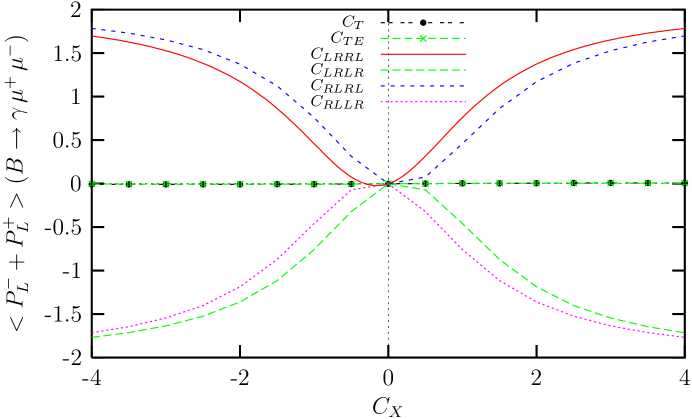
Figure 2: The dependence of the combined averaged longitudinal lepton polarization $<P^{-}_{L}+P^{+}_{L}>$ for the $B_{s}\rightarrow\gamma\,\mu^{+}\mu^{-}$ decay on the new Wilson coefficients .

In Figs. (1) and (2), we present the dependence of the averaged longitudinal polarization $<P^{-}_{L}>$ of $\ell^{-}$ and the combination $<P^{-}_{L}+P^{+}_{L}>$ for $B_{s}\rightarrow\gamma\mu^{+}\mu^{-}$ decay on the new Wilson coefficients. From these figures we see that $<P^{-}_{L}>$ is strongly dependent on scalar type interactions with coefficient $C_{RLRL}$ and $C_{LRRL}$, and quite sensitive to the tensor type interactions, while the combined average $<P^{-}_{L}+P^{+}_{L}>$ is mainly determined by scalar interactions only. The fact that values of $<P^{-}_{L}>$ becomes substantially different from the SM value (at $C_{X}=0$) as $C_{X}$ becomes different from zero indicates that measurement of the longitudinal lepton polarization in $B_{s}\rightarrow\gamma\mu^{+}\mu^{-}$ decay can be very useful to investigate new physics beyond the SM. We note that in Fig. (2), we have not explicitly exhibit the dependence on vector type interactions since we have found that $<P^{-}_{L}+P^{+}_{L}>$ is not sensitive them at all. This is what is already expected since vector type interactions are cancelled when the longitudinal polarization asymmetry of the lepton and antilepton is considered together. We also observe from Fig. (2) that $<P^{-}_{L}+P^{+}_{L}>$ becomes almost zero at $C_{X}=0$, which confirms the SM result, and its dependence on $C_{X}$ is symmetric with respect to this zero point. It is interesting to note also that $<P^{-}_{L}+P^{+}_{L}>$ is positive for all values of $C_{RLRL}$ and $C_{LRRL}$, while it is negative for remaining scalar type interactions .

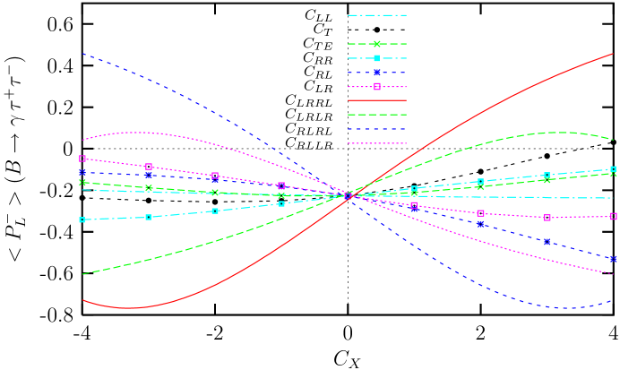
Figure 3: The same as Fig.(1), but for the $B_{s}\rightarrow\gamma\,\tau^{+}\tau^{-}$ decay .

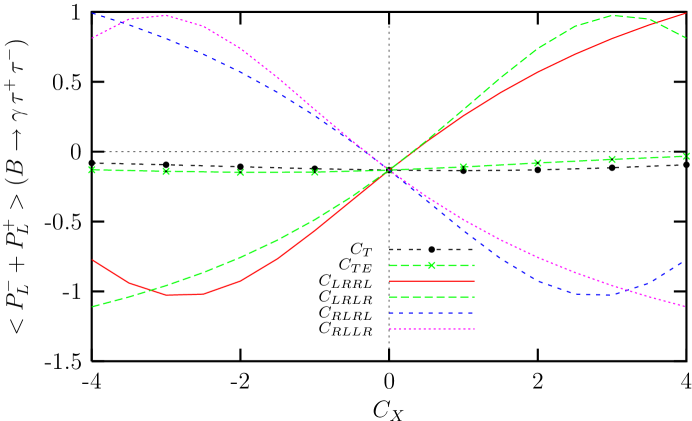
Figure 4: The same as Fig.(2), but for the $B_{s}\rightarrow\gamma\,\tau^{+}\tau^{-}$ decay.

Figs. (3) and (4) are the same as Figs. (1) and (2), but for the $B_{s}\rightarrow\gamma\tau^{+}\tau^{-}$ decay. Similar to the muon case, $<P^{-}_{L}>$ is sensitive to scalar type interactions, but all type. It is an decreasing (increasing) function of $C_{RLRL}$ and $C_{RLLR}$ ($C_{LRRL}$ and $C_{LRLR}$). The value of $<P^{-}_{L}>$ is positive when $C_{RLRL}\stackrel{{\scriptstyle<}}{{{}_{\sim}}}-1$, $C_{RLLR}\stackrel{{\scriptstyle<}}{{{}_{\sim}}}-2$, $C_{LRRL}\stackrel{{\scriptstyle>}}{{{}_{\sim}}}1$ and $C_{LRLR}\stackrel{{\scriptstyle>}}{{{}_{\sim}}}2$. As seen from Fig. (4) that the behavior of the combined average $<P^{-}_{L}+P^{+}_{L}>$ for $B_{s}\rightarrow\gamma\tau^{+}\tau^{-}$ decay is different from the muon case in that it changes sing for a given scalar type interaction: e.g., $<P^{-}_{L}+P^{+}_{L}>>0$ when $C_{RLRL},C_{RLLR}\stackrel{{\scriptstyle<}}{{{}_{\sim}}}0$, while $<P^{-}_{L}+P^{+}_{L}><0$ when $C_{RLRL},C_{RLLR}\stackrel{{\scriptstyle>}}{{{}_{\sim}}}0$. Therefore, it can provide valuable information about the new physics to determine the sign and the magnitude of $<P^{-}_{L}>$ and $<P^{-}_{L}+P^{+}_{L}>$.

In Figs. (5) and (6), the dependence of the averaged transverse polarization $<P^{-}_{T}>$ of $\ell^{-}$ and the combination $<P^{-}_{T}-P^{+}_{T}>$ for $B_{s}\rightarrow\gamma\mu^{+}\mu^{-}$ decay on the new Wilson coefficients are presented. We see from Fig. (5) that $<P^{-}_{T}>$ strongly depends on the scalar interactions with coefficient $C_{RLRL}$ and $C_{LRRL}$ and quite weakly on the all other Wilson coefficients. It is also interesting to note that $<P^{-}_{T}>$ is positive (negative) for the negative (positive) values of $C_{LRRL}$, except a small region about the zero values of the coefficient, while its behavior with respect to $C_{RLRL}$ is opposite. As being different from $<P^{-}_{T}>$ case, in the combination $<P^{-}_{T}-P^{+}_{T}>$ there appears strong dependence on scalar interaction with coefficients $C_{RLLR}$ and $C_{LRLR}$ too, as well as on $C_{RLRL}$ and $C_{LRRL}$. It is also quite sensitive to the tensor interaction with coefficient $C_{T}$.

Figs. (7) and (8) are the same as Figs. (5) and (6), but for the $B_{s}\rightarrow\gamma\tau^{+}\tau^{-}$ decay. As in the muon case, for $\tau$ channel too, the dominant contribution to the transverse polarization comes from the scalar interactions, but it exhibits a more sensitive dependence to the remaining types of interactions as well than the muon case. As seen from Fig. (8) that $<P^{-}_{T}-P^{+}_{T}>$ is negative for all values of the new Wilson coefficients, while $<P^{-}_{T}>$ again changes sign depending on the change in the new Wilson coefficients: e.g., $<P^{-}_{T}>>0$ only when $C_{LRRL}\stackrel{{\scriptstyle<}}{{{}_{\sim}}}-2$ and $C_{RLRL},C_{LR}\stackrel{{\scriptstyle>}}{{{}_{\sim}}}2$. Remembering that in SM in massless lepton case, $<P^{-}_{T}>\approx 0$ and $<P^{-}_{T}-P^{+}_{T}>\approx 0$, determination of the sign of these observables can give useful information about the existence of new physics.

In Figs. (9) and (10), we present the dependence of the averaged normal polarization $<P^{-}_{N}>$ of $\ell^{-}$ and the combination $<P^{-}_{N}+P^{+}_{N}>$ for $B_{s}\rightarrow\gamma\mu^{+}\mu^{-}$ decay on the new Wilson coefficients. We observe from these figures that behavior of both $<P^{-}_{N}>$ and $<P^{-}_{N}+P^{+}_{N}>$ are determined by tensor type interactions with coefficient $C_{TE}$. They both are positive (negative) when $C_{TE}\stackrel{{\scriptstyle<}}{{{}_{\sim}}}0$ ($C_{TE}\stackrel{{\scriptstyle>}}{{{}_{\sim}}}0$).

Figs. (11) and (12) are the same as Figs. (9) and (10), but for the $B_{s}\rightarrow\gamma\tau^{+}\tau^{-}$ decay. As being different from the muon case, $<P^{-}_{N}>$ for $\tau$ channel is also sensitive to the vector type interaction with coefficient $C_{LL}$, as well as the tensor types and it is negative for all values of the new Wilson coefficients. As for the combination $<P^{-}_{N}+P^{+}_{N}>$ for $\tau$ channel, it is negative too for all values of $C_{X}$, except for $C_{TE}\stackrel{{\scriptstyle<}}{{{}_{\sim}}}-2$.

We now summarize our results:

• $<P^{-}_{L}>$ and $<P^{-}_{T}>$ are strongly dependent on scalar type interactions with coefficient $C_{RLRL}$ and $C_{LRRL}$, while $<P^{-}_{N}>$ is mainly determined by tensor type interactions with coefficient $C_{TE}$.

• Measurement of $<P^{-}_{L}>$ in $B_{s}\rightarrow\gamma\mu^{+}\mu^{-}$ decay can be very useful to investigate new physics beyond the SM since it becomes substantially different from the SM value (at $C_{X}=0$) as $C_{X}$ becomes different from zero.

• The combined averages $<P^{-}_{L}+P^{+}_{L}>$ and $<P^{-}_{T}-P^{+}_{t}>$ are mainly determined by scalar interactions only. As for the $<P^{-}_{N}+P^{+}_{N}>$, it is quite sensitive to tensor type interactions with coefficient $C_{TE}$.

• $<P^{-}_{L}+P^{+}_{L}>$ becomes almost zero at $C_{X}=0$, which confirms the SM result and it is positive for all values of $C_{RLRL}$ and $C_{LRRL}$, while it is negative for remaining scalar type interactions.

• Since in the SM in massless lepton case, $<P^{-}_{T}>\approx 0$ and $<P^{-}_{T}-P^{+}_{T}>\approx 0$, determination of the sign of these observables can give useful information about the existence of new physics.

In conclusion, we have studied the lepton polarizations in the rare $B_{s}\rightarrow\gamma\,\ell^{+}\ell^{-}$ decays by using the general, model independent form of the effective Hamiltonian. The sensitivity of the longitudinal, transverse and normal polarizations of $\ell^{-}$, as well as lepton-antilepton combined asymmetries, on the new Wilson coefficients are investigated. We find that all these physical observables are very sensitive to the existence of new physics beyond SM and their experimental measurements can give valuable information about it.

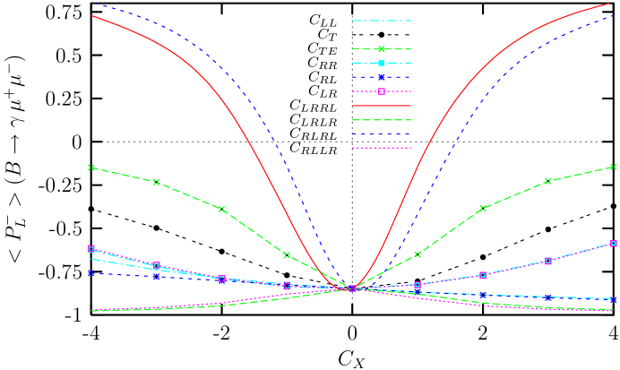
Figure 1: The dependence of the averaged longitudinal polarization $<P^{-}_{L}>$ of $\ell^{-}$ for the $B_{s}\rightarrow\gamma\,\mu^{+}\mu^{-}$ decay on the new Wilson coefficients .

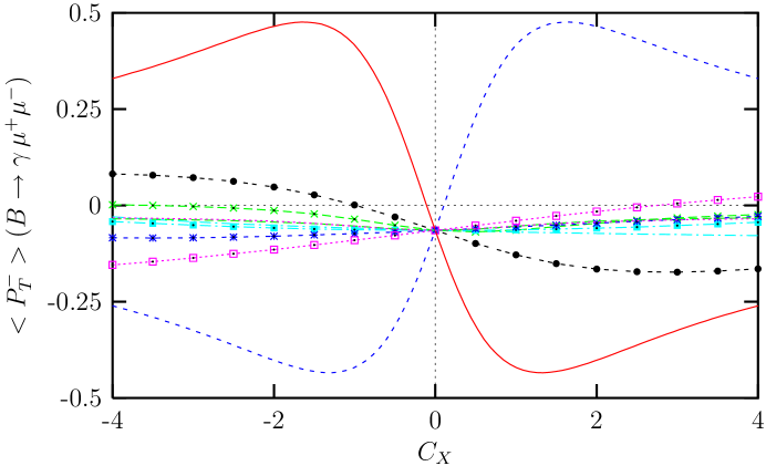
Figure 5: The dependence of the averaged transverse polarization $<P^{-}_{T}>$ of $\ell^{-}$ for the $B_{s}\rightarrow\gamma\,\mu^{+}\mu^{-}$ decay on the new Wilson coefficients. The line convention is the same as before.

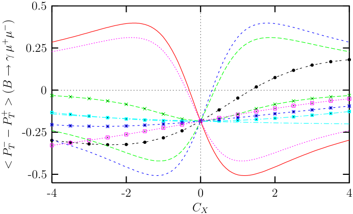
Figure 6: The dependence of the combined averaged transverse lepton polarization $<P^{-}_{T}-P^{+}_{T}>$ for the $B_{s}\rightarrow\gamma\,\mu^{+}\mu^{-}$ decay on the new Wilson coefficients. The line convention is the same as before.

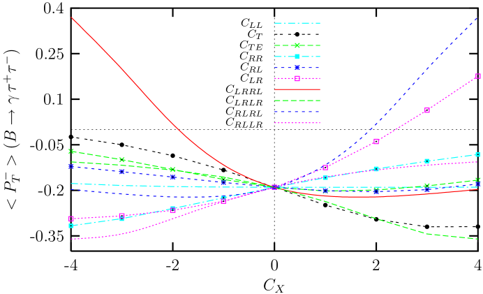
Figure 7: The same as Fig.(5), but for the $B_{s}\rightarrow\gamma\,\tau^{+}\tau^{-}$ decay.

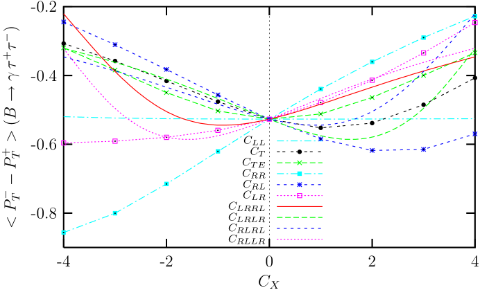
Figure 8: The same as Fig.(6), but for the $B_{s}\rightarrow\gamma\,\tau^{+}\tau^{-}$ decay.

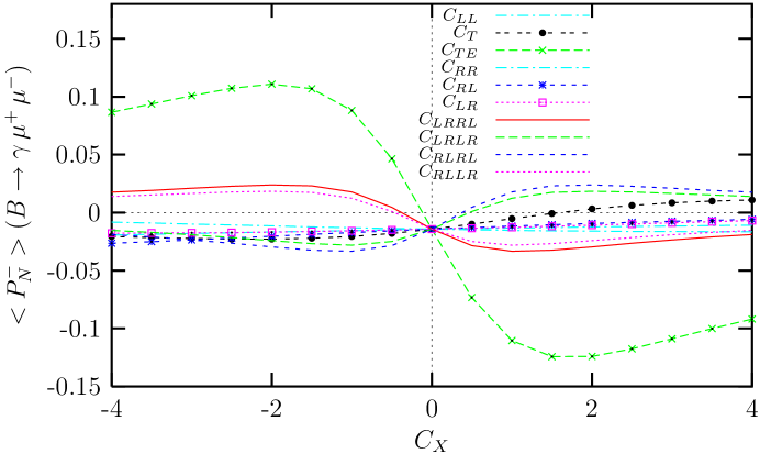
Figure 9: The dependence of the averaged normal polarization $<P^{-}_{N}>$ of $\ell^{-}$ for the $B_{s}\rightarrow\gamma\,\mu^{+}\mu^{-}$ decay on the new Wilson coefficients .

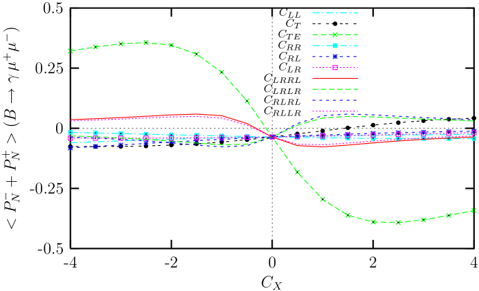
Figure 10: The dependence of the combined averaged normal lepton polarization $<P^{-}_{N}+P^{+}_{N}>$ for the $B_{s}\rightarrow\gamma\,\mu^{+}\mu^{-}$ decay on the new Wilson coefficients.

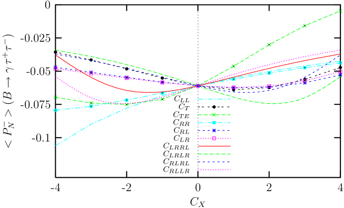
Figure 11: The same as Fig.(9), but for the $B_{s}\rightarrow\gamma\,\tau^{+}\tau^{-}$ decay.

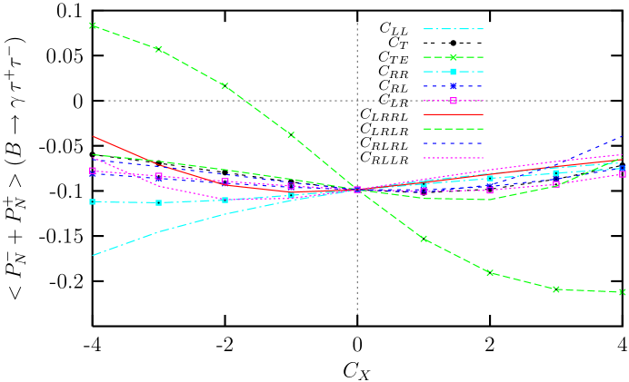
Figure 12: The same as Fig.(10), but for the $B_{s}\rightarrow\gamma\,\tau^{+}\tau^{-}$ decay.

References

• [1] For a recent review see T. Hurth, Rev. Mod. Phys., 75, (2003) 1159.
• [2] G. Burdman, T. Goldman and D. Wyler, Phys. Rev., D 51 (1995) 111;
• [3] G. Eilam, I. Halperin and R. Mendel, Phys. Lett., B 361(1995) 137.
• [4] D. Atwood, G. Eilam and A. Soni Mod. Phys. Lett., A11, (1996)1061.
• [5] P. Colangelo, F. De Fazio, G. Nardulli, Phys. Lett., B372,(1996) 331.
• [6] T. Aliev, A. Γ–zpineci and M. Savci, Phys. Lett., B393, (1997)143.
• [7] T. Aliev, A. Γ–zpineci and M. Savci, Phys. Rev., D55, (1997) 7059 .
• [8] T. M. Aliev, N. K. Pak, and M.SavcΔ±, Phys. Lett. B 424 (1998) 175.
• [9] C. Q. Geng, C. C. Lih and W. M. Zhang, Phys. Rev., D57 (1998) 5697.
• [10] C. C. Lih, C. Q. Geng and W. M. Zhang, Phys. Rev., D59 (1999) 114002.
• [11] G. P. Korchemsky, Dan Pirjol and Tung-Mow Yan, Phys.Rev., D61 (2000) 114510.
• [12] G. Eilam, C.-D. LΓΌ and D.-X. Zhang, Phys. Lett. B391, (1997)461.
• [13] C. Q. Geng, C. C. Lih and W. M. Zhang, Phys. Rev., D62 (2000) 074017.
• [14] F. Kruger and D. Melikhov, Phys. Rev. D 67 (2003) 034002.
• [15] Z. Xiong and J. M.Yang, Nucl. Phys. B 628 (2002) 193.
• [16] S. R. Choudhury, and N. Gaur, hep-ph/0205076.
• [17] S. R. Choudhury, and N. Gaur, hep-ph/0207353.
• [18] S. R. Choudhury, N. Gaur, and N. Mahajan, Phys. Rev. D 66 (2002) 054003.
• [19] E. O. Iltan and G. Turan, Phys. Rev. D 61 (2000) 034010.
• [20] T. M. Aliev, A. Γ–zpineci and M. SavcΔ±,Phys. Lett. B 520 (2001) 69.
• [21] G. Erkol and G. Turan, Phys. Rev. D 65 (2002) 094029.
• [22] G. Erkol and G. Turan, Acta Phys. Pol. B 33, No:5, (2002)1285.
• [23] U. O. YΔ±lmaz, B. B. ŞirvanlΔ± and G. Turan, Eur. Phys. J. C 30 (2003) 197.
• [24] S. Fukae, C. S. Kim, T. Morozumi and T. Yoshikawa, Phys. Rev. D59 (1999) 074013. T. M. Aliev, C. S. Kim, Y. G. Kim, Phys. Rev. D62 (2000) 014026; T. M. Aliev, D. A. Demir, M. SavcΔ±, Phys. Rev. D62 (2000) 074016;
• [25] S. Fukae, C. S. Kim and T. Yoshikawa, Phys. Rev. D61 (2000) 074015.
• [26] T. M. Aliev, M. K. Γ‡akmak and M. SavcΔ±, Nucl. Phys. B 607 (2001) 305; T. M. Aliev, M. K. Γ‡akmak, A. Γ–zpineci and M. SavcΔ±, Phys. Rev. D64 (2001) 055007;
• [27] A. J. Buras and M. MΓΌnz,Phys. Rev. D 52 (1995) 186; M. Misiak, Nucl. Phys., B 393(1993) 23; erratum ibid. B 439 (1995) 461.
• [28] A. Ali, T. Mannel and T. Morozumi, Phys. Lett. B 273 (1991) 505;
• [29] K. Abe, et al., BELLE Collaboration, Phys. Rev. Lett. 88 (2002) 021801; B. Aubert, et al., BaBar Collaboration, Phys. Rev. Lett. 88 (2002) 241801.
• [30] V. Halyo,hep-ex/0207010.
• [31] Chao-Shang Huang and Xiao-Hong Wu, Nucl. Phys. B 665 (2003) 304.
Refer to caption