The Neutron Electric Dipole Moment in the Instanton Vacuum:
Quenched Versus Unquenched Simulations

Abstract

We investigate the role played by the fermionic determinant in the evaluation of the $CP$-violating neutron electric dipole moment (EDM) adopting the Instanton Liquid Model. Significant differences between quenched and unquenched calculations are found. In the case of unquenched simulations the neutron EDM decreases linearly with the quark mass and is expected to vanish in the chiral limit. On the contrary, within the quenched approximation, the neutron EDM increases as the quark mass decreases and is expected to diverge as $1/m^{N_{f}}$ in the chiral limit. We argue that such a qualitatively different behavior is a parameter-free, semi-classical prediction and occurs because the neutron EDM is sensitive to the topological structure of the vacuum. The present analysis suggests that quenched and unquenched lattice QCD simulations of the neutron EDM as well as of other observables governed by topology might show up important differences in the quark mass dependence, for $m_{q}\lesssim\Lambda_{QCD}$.

1 Introduction

The electric dipole moment (EDM) of the neutron provides direct information on the violation of the parity and time-reversal symmetries. Both the strong and the electroweak sectors of the Standard Model (SM) can generate violations of the above symmetries. As for the strong sector, it is known tHooft that a gauge-invariant definition of the QCD vacuum requires to supplement the classical action with an additional gauge-invariant and renormalizable term, which in Euclidean space reads

$$\mathcal{S}_{QCD}^{\prime} = \mathcal{S}_{QCD}~{}+~{}\mathcal{S}_{\theta}~{},$$ (1.1)

$$\mathcal{S}_{\theta} = i~{}\theta~{}\frac{1}{32\pi^{2}}\int d^{4}x~{}F_{\mu\nu}\widetilde{F}_{\mu\nu}~{},$$ (1.2)

where

$$Q=\frac{1}{32\pi^{2}}\int d^{4}x~{}F_{\mu\nu}\widetilde{F}_{\mu\nu}$$ (1.3)

is the topological charge operator, $\widetilde{F}_{\mu\nu}=(1/2)~{}\varepsilon_{\mu\nu\alpha\beta}F_{\alpha\beta}$ is the dual gluon field strength (incorporating the strong coupling constant) and $\theta$ is a (real) dimensionless parameter. The term (1.2) is a source of $CP$ violation and goes under the name of strong $\theta$-term.

A second independent physical origin for a term of the form (1.2) comes from the weak sector of the SM. The observation of $CP$ violation in K-meson systems implies that the quark mass matrix $M$ is not real and the mass term in the Lagrangian has the general form

$$\mathcal{L}_{M}=\overline{\psi}_{i}^{R}~{}M_{ij}~{}\psi^{L}+\overline{\psi}_{i}^{L}~{}M_{ij}^{\dagger}~{}\psi^{R}~{}.$$ (1.4)

The mass matrix can be made real and diagonal by means of an appropriate chiral rotation, which generates a shift in the $\theta$ parameter:

$$\theta\rightarrow\overline{\theta}\doteq\theta+\textrm{argdet}(M)~{}.$$ (1.5)

The real constant $\overline{\theta}$ is an additional dimensionless parameter, which has to be fixed from experiment. This can be done by exploiting the fact that (1.2) is a source of $CP$ violation which leads to a non-vanishing value of the neutron EDM. At present there are only upper bounds on the neutron EDM and the most constraining one is $|\mathbf{d}_{n}|<6.3\times 10^{-13}~{}(\mathrm{e\cdot fm})$ ILL .

In order to translate this experimental information into a constraint on $\overline{\theta}$, one needs to compute the neutron EDM in QCD, including the contribution of the topological term $i{\overline{\theta}~{}Q}$. So far, this has been done only within model-dependent frameworks, starting from the works of Refs. Baluni ; Crewther . In Baluni Baluni performed a calculation of the EDM in the Bag Model and found $|\mathbf{d}_{n}|=2.7\times 10^{-3}~{}\overline{\theta}~{}(\mathrm{e\cdot fm})$. In Crewther Crewther et al. proposed an approach based on current algebra relations and found $|\mathbf{d}_{n}|=3.6\times 10^{-3}~{}\overline{\theta}~{}(\mathrm{e\cdot fm})$.

The above model calculations agree in pointing out that $|\overline{\theta}|\lesssim 2\cdot 10^{-10}$. Understanding why $\overline{\theta}$ is so small is an open challenge, which goes under the name of strong $CP$ problem.

In order to estimate the relevant matrix element in a model-independent way, a non-perturbative approach based on the fundamental theory, like lattice QCD, is required. However a lattice estimate of the neutron EDM is not yet available Aoki . Recently Diego a new strategy for computing the neutron EDM in lattice QCD has been proposed. The starting point is the expansion of the matrix element of the EDM operator to lowest order in $\overline{\theta}$. This allows to remove the complex $\theta$-term (1.2) from the action, but at the expense of calculating the matrix element of a composite operator made of the electromagnetic dipole and the topological charge operators:

$$\mathbf{d}_{n} = \langle N(\overline{\theta})|\int d\mathbf{x\,\,x\,}J_{0}(\mathbf{x)}|N(\overline{\theta})\rangle$$

$$\simeq -i~{}\overline{\theta}\,\,\langle N(0)|\int d\mathbf{x\,\,x\,}J_{0}(\mathbf{x)}$$

$$\cdot \left[\frac{1}{32\pi^{2}}\int d^{4}z~{}F_{\mu\nu}\widetilde{F}_{\mu\nu}\right]|N(0)\rangle$$ (1.7)

where $|N(\overline{\theta})\rangle$ denotes the neutron state at a finite value of $\overline{\theta}$.

Computing the matrix element (1.7) on the lattice is a very challenging task. The main source of difficulties is that the topological charge operator is very noisy Gockeler . A possible way-out, suggested in Refs. Aoki ; Diego , consists in exploiting the anomalous Ward identities to replace the topological charge operator in (1.7) with the pseudo-scalar density operator, namely

$$\langle\mathcal{O}\left[\frac{2N_{f}}{32\pi^{2}}\int d^{4}z~{}F_{\mu\nu}\widetilde{F}_{\mu\nu}\right]\rangle=$$

$$-2m_{0}~{}\langle\mathcal{O}\int d^{4}z~{}P(z)\rangle_{disc.}~{},$$ (1.8)

where $\langle~{}\rangle$ denotes the quantum average over all configurations, $N_{f}$ is the number of quark flavors, $m_{0}$ is the bare quark mass ($1/m_{0}\equiv(1/m_{u}+1/m_{d}+1/m_{s})/3$ for $N_{f}=3$) and $P$ is the flavor-singlet pseudo-scalar operator $P(x)=\sum_{f}\overline{\psi}_{f}(x)\gamma_{5}\psi_{f}(x)$. In the r.h.s. of Eq. (1.8) $\langle~{}\rangle_{disc}$ denotes the quantum average obtained by retaining only the Wick contractions in which the pseudo-scalar operator is contracted in a virtual quark loop. The numerical applicability of such a strategy is still under investigation.

The use of the quenched approximation is quite natural for a first-time calculation. We point out however that neglecting the fermionic determinant may result in a sizable systematic error in case of the neutron EDM, since the evaluation of the latter involves flavor-singlet operators. Indeed, in case of hadron masses and decay constants quenched calculations turn out to be accurate, since they appear to agree with available (partially) unquenched simulations within $5\div 10\%$ accuracy CP-PACS ; Davies . However, in case of observables which are directly related to the topological properties of the vacuum, the contribution of the fermionic determinant may become more important.

This can be seen, for example, by considering the Index Theorem, according to which the total topological charge of a gauge configuration relates to the difference of the number of left- and right-handed zero-modes of the Dirac operator:

$$Q=n_{L}-n_{R}~{}.$$ (1.9)

On the other hand, the fermionic determinant can be written in terms of eigenvalues of the Dirac operator as:

$$\mathrm{det}(D{\hskip-6.25958pt}/+m_{f})=m^{\nu}\prod_{\lambda>0}(\lambda^{2}+m_{f}^{2})~{},$$ (1.10)

where $D{\hskip-6.25958pt}/\,\psi_{\lambda}=\lambda\,\psi_{\lambda}$, and $\nu$ is the number of zero-modes.

Equations (1.9) and (1.10) imply that, for small values of the bare quark masses, the fermionic determinant suppresses configurations with a non-vanishing topological charge. Since the EDM is an observable which relates directly to topology, we argue that evaluating this quantity in quenched and unquenched lattice QCD might lead to quite different results. Of course, one can still hope that sufficiently away from the chiral limit quenched and full simulations give comparable results.

While waiting for lattice results on the neutron EDM, the aim of this work is to investigate the role played by the fermionic determinant using a model which is expected to take into account properly topological effects. Such a model is the Instanton Liquid Model (ILM), since instantons are topological gauge configurations which dominate the QCD Path Integral in the semi-classical limit. They generate the so-called ’t Hooft interaction, that solves the U(1) problem tHooft and spontaneously breaks chiral symmetry dyakonov , but does not confine. Evidence for such an instanton-induced interaction in QCD comes from a number of phenomenological studies shuryakrev , as well as from lattice simulations chu94 ; Degrand ; scalar . The ILM assumes that the QCD vacuum is saturated by an ensemble of instantons and anti-instantons. The only phenomenological parameters in the model are the instanton average size and density. Their values were estimated long ago from the global vacuum properties shuryak82 . Since this model provides very successful descriptions of both the pion and nucleon electromagnetic structure nucleonFF and of the topological properties of the QCD vacuum toposcreening , we expect its prediction for the neutron EDM to be realistic.

The dynamical mechanism leading to the formation of the neutron EDM in the instanton vacuum was recently investigated by one of the author bnumber . It was found that, during the tunneling processes, the $\theta$-term generates an effective repulsion between matter and anti-matter, in the neutron. As a consequence, quarks and anti-quarks migrate in opposite directions. Hence, at least on the semi-classical level, the EDM arises from the local separation of positive and negative baryonic charges in the neutron. It does not follow from the displacement of the positive and negative electric charge carried by the valence quarks, as one would intuitively expect in a naive non-relativistic quark model picture.

In this work we show that the use of the ILM clearly suggests that neglecting the fermionic determinant leads to a dangerous divergence in the chiral limit, which in the full model is regulated by topological screening. We will compare unquenched and quenched model calculations at values of the space-time volume and of the current quark mass which are comparable to those used in present-day lattice simulations, and provide numerical estimates of the neutron EDM.

In order to model quenched and full QCD, we will use the Interacting Instanton Liquid Model (IILM) developed by Shuryak and collaborators (see Ref. shuryakrev for a review). In this model the configurations of the instanton ensemble are generated by means of a Metropolis algorithm which explicitly accounts for the fermionic determinant. The instanton size distribution is not fixed a priori, but it is obtained dynamically. The average density was fixed by minimizing the free energy IILM . In the IILM the neglect of the fermionic determinant generates pathologies which are analogous to the ones observed in quenched lattice QCD (see Ref. scalar ).

The feasibility of instanton calculations relies on two important simplifications, which arise when one restricts the functional integration over the gauge field configurations to an ordinary integral over the collective coordinates of an ensemble of $N_{+}$ instanton and $N_{-\;}$anti-instantons. On the one hand, one has to deal with a dramatically smaller number of degrees of freedom, typically of the order of $12\times(N_{+}+N_{-})\sim 10^{3}$ (for a typical box of the size of those used in lattice simulations). On the other hand, evaluating the topological charge operator in the instanton vacuum is trivial, because it amounts to simply counting the number of instantons and anti-instantons in the ensemble (indeed $Q=N_{+}-N_{-}$ ). Due to these simplifications, the numerical simulations leading to the EDM can be performed on a regular workstation.

We show that, within the IILM, quenched simulations become unreliable for quark masses smaller than the strange quark mass. Indeed, for $m_{q}\gtrsim 200$ MeV, quenched and full simulations give results which agree within statistical errors, whereas for quark masses of the order of $100$ MeV, quenched calculations overestimate the EDM by a factor $\simeq 4$. This is due to the appearance of the chiral divergence mentioned previously. Moreover, we stress that other quantities, like e.g. the nucleon mass or the quark condensate, are not drastically affected by quenching.

Assuming a linear mass dependence, the extrapolation of the unquenched ILM results to a physical value of the light quark mass between 4 and 10 MeV yields: $|{\bf d}_{n}|=(6\div 14)\times 10^{-3}~{}\overline{\theta}$ (e $\cdot$ fm), which is a factor about $2\div 4$ larger than the estimates obtained in Refs. Baluni ; Crewther .

The paper is organized as follows. In Section 2 we shall discuss our method for relating the neutron EDM to Euclidean correlation functions. In Section 3 we will study these correlators in the instanton vacuum and derive the quenched and unquenched expressions for the neutron EDM. In Section 4 we analyze the chiral behavior both for quenched and unquenched calculations. Results are presented and discussed in Section 5, and, finally, conclusions are summarized in Section 6.

2 Relating the neutron EDM to euclidean correlation functions

To compute the neutron EDM in a field-theory framework, we start by considering the following Euclidean correlation function:

$$D_{\tau}^{\gamma\gamma^{\prime}}(\mathbf{p,q)} \doteq \int d\mathbf{x}\int d\mathbf{y}e^{i\mathbf{px}+i\mathbf{qy}}y_{3}G_{\tau}^{\gamma\gamma^{\prime}}(\mathbf{x,y)}$$

$$= -i\frac{\partial}{\partial q_{3}}\int d\mathbf{x}\int d\mathbf{y}e^{i\mathbf{px}+i\mathbf{qy}}G_{\tau}^{\gamma\gamma^{\prime}}(\mathbf{x,y})~{},~{}~{}~{}~{}$$

$$G_{\tau}^{\gamma\gamma^{\prime}}(\mathbf{x,y)} \doteq \langle 0|T[J_{N}^{\gamma}(\mathbf{0},2\tau)J_{4}(\mathbf{y},\tau)\overline{J}_{N}^{\gamma^{\prime}}(\mathbf{x},0)|0\rangle$$ (2.12)

where $J_{N}^{\gamma}(x)=\varepsilon_{abc}(u^{T}_{a}C\gamma_{5}d_{b})d_{c}^{\gamma}$ is an interpolating operator for the neutron, $p=(\mathbf{p},\omega)$, $p^{\prime}=(\mathbf{p}+\mathbf{q},\omega^{\prime})$. In the limit of large Euclidean times $\tau$ one can show that:

$$D_{\tau}^{\gamma\gamma^{\prime}}(\mathbf{p,q)} \stackrel{{\scriptstyle\tau\rightarrow\infty}}{{\longrightarrow}} -i\frac{\partial}{\partial q_{3}}\left(Z^{2}\frac{1}{2\omega~{}2\omega^{\prime}}e^{-(\omega^{\prime}+\omega)\tau}\right.$$ (2.13)

$$\cdot \left.\left[(p{\hskip-4.83694pt}/^{\prime}+M)~{}\mathrm{K}(q^{2})(p{\hskip-4.83694pt}/+M)\right]^{\gamma\gamma^{\prime}}\right)~{},~{}~{}~{}~{}$$

where $M$ is the mass of the neutron, $Z$ is a constant defined by

$$\langle 0|J_{N}(0)|N(p,s)\rangle=Z~{}u(p,s)~{},$$ (2.14)

where $u(p,s)$ is a Dirac spinor, and

$$\mathrm{K}(q^{2}) = F_{1}(q^{2})~{}\gamma_{4}+iF_{2}(q^{2})~{}\frac{\sigma_{43}}{2M}~{}q_{3}$$ (2.15)

$$+ F_{A}(q^{2})~{}(q^{2}\gamma_{4}-2Mq_{4})~{}\gamma_{5}$$

$$+ F_{3}(q^{2})~{}\frac{\sigma_{43}}{2M}~{}\gamma_{5}~{}q_{3}~{}.$$

with $\sigma_{43}$ the Euclidean version of $\sigma_{03}=i\gamma_{0}\gamma_{3}$. Notice that the form factors $F_{A}(q^{2})$ and $F_{3}(q^{2})$ do not appear if we assume that the matrix element is invariant under $C$, $P$, and $T$. In particular $F_{3}(q^{2}=0)$ relates directly to the EDM through the relationship:

$$D\doteq\frac{|\mathbf{d}_{n}|}{e}=\frac{F_{3}(0)}{2M}~{}.$$ (2.16)

In order to isolate the contribution to the EDM it is convenient to define the following trace:

$$\Sigma_{\tau}(\mathbf{p},\mathbf{q})\doteq\mathrm{Tr}[D_{\tau}(\mathbf{p},\mathbf{q})~{}\Gamma_{3}],\qquad\Gamma_{3}\doteq\left(\begin{array}[]{ll}\sigma_{3}&0\\ 0&\sigma_{3}\end{array}\right)$$ (2.19)

and obtain:

$$\Sigma_{\tau}(\mathbf{p},\mathbf{q}) \longrightarrow -\frac{Z^{2}}{8M}i\frac{\partial}{\partial q_{3}}\Phi_{\tau}(\mathbf{p},\mathbf{q}),$$ (2.20)

$$\Phi_{\tau}(\mathbf{p},\mathbf{q}) = \frac{1}{\omega\omega^{\prime}}~{}e^{-(\omega+\omega^{\prime})\tau}\mathrm{Tr}[(p{\hskip-4.83694pt}/^{\prime}+M)~{}\gamma_{5}~{}\sigma_{43}$$ (2.21)

$$\cdot (p{\hskip-4.83694pt}/+M)\Gamma_{3}]q_{3}~{}F_{3}(q^{2})~{}.$$

Taking $\mathbf{q}=0$ we obtain:

$$\Sigma_{\tau}(\mathbf{p,q=0})\stackrel{{\scriptstyle\tau\rightarrow\infty}}{{\longrightarrow}}-2Z^{2}e^{-2\omega\tau}\frac{p_{1}^{2}+p_{2}^{2}}{\mathbf{p}^{2}+M^{2}}~{}D~{}.$$ (2.22)

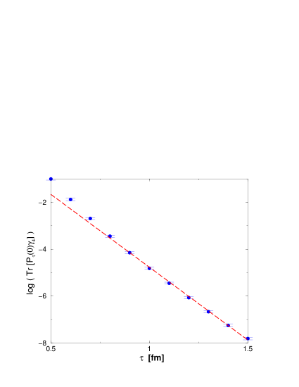
Fig. 1: ILM results for $log(Tr[P_{\tau}({\bf p}={\bf 0})~{}\gamma_{4}])$. The linear behavior denotes the isolation of the nucleon pole. The slope of the line corresponds to the nucleon mass $M$ (in units of inverse fm) while its intercept corresponds to $log(2\,Z^{2})$. These results were obtained in the quenched approximation, by averaging over the configurations of an ensemble of $56$ pseudo-particles in a volume $V=2.4^{3}\times 4=56$ fm⁴ and quark masses of $m_{q}=1.00~{}\Lambda_{QCD}$.

All correlation functions defined so far are projected onto fixed momentum components, hence the spatial position of the sources and of the electromagnetic operator are completely unspecified. From the practical point of view, evaluating these quantities can be very challenging, because they involve a six-dimensional integration over the two spatial hyperplanes. This has to be performed numerically and requires to compute a large number of evaluation points for the integrand, each of which is a three-point correlation function. However, as long as we are interested in a static property of the neutron, such as the EDM, it is possible to reduce the number of spatial integrations by working in a mixed space-momentum representation, where one projects only on the momentum transfer by the photon and leaves the source and the sink at a fixed spatial location. In this way one gives up the information about the initial momentum of the neutron. Let us define the correlator:

$$\widetilde{\Sigma}_{\tau}(\mathbf{x},\mathbf{q}=\mathbf{0)=}\int\frac{d\mathbf{p}}{(2\pi)^{3}}~{}e^{-i\mathbf{p\,x}}\Sigma_{\tau}(\mathbf{p},\mathbf{q}=\mathbf{0})~{}.$$ (2.23)

Choosing $\mathbf{x}=\mathbf{0}$ we obtain:

$$\widetilde{\Sigma}_{\tau}(\mathbf{x}=\mathbf{0},\mathbf{q}=\mathbf{0)}=\int d\mathbf{y}~{}y_{3}~{}\mathrm{Tr}\mathbf{[}G_{\tau}(\mathbf{x}=\mathbf{0},\mathbf{y})~{}\Gamma_{3}]$$

$$\stackrel{{\scriptstyle\tau\rightarrow\infty}}{{\longrightarrow}}D\times\left(-2Z^{2}\int\frac{d\mathbf{p}}{(2\pi)^{3}}~{}e^{-2\omega\tau}~{}\frac{p_{1}^{2}+p_{2}^{2}}{\mathbf{p}^{2}+M^{2}}~{}\right)~{}.~{}$$ (2.24)

Evaluating $\widetilde{\Sigma}_{\tau}(\mathbf{x}=\mathbf{0},\mathbf{q}=\mathbf{0})$ involves only a three-dimensional integration over the position of the electromagnetic current. Moreover, the number of independent numerical integrations can be further reduced to two, by exploiting the rotational symmetry of $G_{\tau}(\mathbf{x}=\mathbf{0},\mathbf{y})$ around the $y_{3}$ axis:

$$\widetilde{\Sigma}_{\tau}(\mathbf{x}=\mathbf{0},\mathbf{q}=\mathbf{0}) = 2\pi\int_{-\infty}^{\infty}dy_{3}~{}y_{3}~{}\int d|\mathbf{y}_{\perp}|~{}|\mathbf{y}_{\perp}|$$ (2.25)

$$\cdot \mathrm{Tr}[G_{\tau}(\mathbf{x}=\mathbf{0},\mathbf{y})~{}\Gamma_{3}]~{}.$$

As usual, the neutron mass $M$ and the coupling $Z$ to the neutron interpolating operator appearing in the r.h.s. of Eq. (2.24) can be extracted from the zero momentum two-point correlator,

$$P_{\tau}^{\gamma\gamma^{\prime}}(\mathbf{p}=\mathbf{0}) = \int d\mathbf{x}\langle 0|T[J_{N}^{\gamma}(\mathbf{x},\tau)\overline{J}_{N}^{\gamma^{\prime}}(\mathbf{0},0)|0\rangle$$ (2.26)

$$\stackrel{{\scriptstyle\tau\rightarrow\infty}}{{\longrightarrow}} Z^{2}\frac{(1+\gamma_{4})^{\gamma\gamma^{\prime}}}{2}e^{-M\tau}~{}.$$

3 The neutron EDM in the instanton vacuum

In QCD the neutron EDM is non-zero only at finite values of the $\overline{\theta}$-angle. To lowest order in this parameter the three-point correlation function (2.12) reads:

$$G_{\tau}^{\gamma\gamma^{\prime}}(\mathbf{x,y)} = i\overline{\theta}\langle 0|T[J_{N}^{\gamma}(\mathbf{0},2\tau)J_{4}(\mathbf{y},\tau)\overline{J}_{N}^{\gamma^{\prime}}(\mathbf{x},0)$$ (3.27)

$$\cdot \frac{1}{32\pi^{2}}\int d^{4}z~{}F_{\mu\nu}(z)~{}\widetilde{F}_{\mu\nu}(z)]|0\rangle~{},~{}~{}~{}~{}$$

where $|0\rangle$ refers to the vacuum at $\overline{\theta}=0$.

In the instanton vacuum the topological charge is condensed around instantons and anti-instantons, and correlation functions are computed by averaging over the configurations of a grand-canonical ensemble of such pseudo-particles with a partition function given by:

$$\mathcal{Z}(\mu,\overline{\theta}) = \sum_{N_{+},N_{-}}e^{(\mu+i\overline{\theta})~{}N_{+}+(\mu-i\overline{\theta})~{}N_{-}}~{}Z_{N_{+}N_{-}}$$ (3.28)

$$Z_{N_{+}N_{-}} = \frac{1}{N_{+}!N_{-}!}\prod_{i=1}^{N_{+}+N_{-}}\int d^{4}z_{i}d\rho_{i}dU_{i}d(\rho_{i})$$ (3.29)

$$\cdot \prod_{f}\mathrm{det(}D{\hskip-6.25958pt}/+m_{f}\mathrm{)\,}~{}e^{-S_{int}}~{}.$$

In this formula $S_{int}$ is the bosonic instanton-instanton interaction, $z_{i}$ denotes the position of the pseudo-particle of size $\rho_{i}$, $dU_{i}$ is the Haar measure normalized to unity and $d(\rho_{i})$ is the instanton size distribution. For small-sized instantons, such a distribution can be calculated by integrating over small gaussian quantum fluctuations around the instanton solution. At two loops, ’t Hooft originally found:

$$d(\rho) = \frac{0.466e^{-1.679N_{c}}}{(N_{c}-1)!(N_{c}-2)!}\left(\frac{8\pi^{2}}{g^{2}(\rho)}\right)^{2N_{c}}$$ (3.30)

$$\cdot \exp\left(-\frac{8\pi^{2}}{g^{2}(\rho)}\right)\frac{1}{\rho^{5}}~{}.$$

As the size of the instanton increases, the overlapping with the field of other pseudo-particles becomes not negligible. This generates interaction between pseudo-particles which dynamically suppresses the instanton weight $d(\rho)$ for large $\rho$. From variational calculations dia , phenomenological estimates shuryak82 and lattice simulations lattice one finds that the $d(\rho)$ is peaked around a mean value $\overline{\rho}=0.3\div 0.5$ fm.

In (3.28) we have introduced a complex chemical potential $(\mu\pm i\overline{\theta}),$ associated with the fluctuations of the number of instantons and anti-instantons in the ensemble. Equivalently, one can rewrite the partition function in (3.28) as a sum over the total topological charge and total number of pseudo-particles:

$$\mathcal{Z}(\mu,\overline{\theta}) = \sum_{Q=0,\pm 1,...}\sum_{N=1,2,...}e^{\mu N+i\overline{\theta}Q}Z_{QN}$$ (3.31)

$$Q \doteq N_{+}-N_{-}~{},$$ (3.32)

$$N \doteq N_{+}+N_{-}~{}.$$ (3.33)

From this equation it follows that $i\overline{\theta}$ can be interpreted as an imaginary chemical potential associated to the fluctuations of the topological charge.

The relative width of the fluctuations of $N$ and $Q$ around their mean values is proportional to the inverse of the size of the system. Thus, in the thermodynamic limit, such fluctuations have no consequences on quantities that are intensive in $N$ and $Q$. Hence observables such as the nucleon mass can be reliably calculated assuming $N=\langle N\rangle$ and $Q=\langle Q\rangle=0$. On the contrary fluctuations can never be neglected when computing averages of operators which are extensive in $N$ or $Q$, like the case of the correlation function (3.27).

Since in the ILM topology is clustered around instantons and anti-instantons, a generic matrix element of the type

$$\langle 0|\mathcal{O}\frac{1}{32\pi^{2}}\int d^{4}zF_{\mu\nu}\widetilde{F}_{\mu\nu}|0\rangle$$ (3.34)

can be written as DPW96

$$\left\langle\mathcal{O}\frac{1}{32\pi^{2}}\int d^{4}zF_{\mu\nu}\widetilde{F}_{\mu\nu}\right\rangle=\sum_{Q}\mathcal{P}(Q)~{}Q\left\langle\mathcal{O}\right\rangle_{Q}~{},$$ (3.35)

where $\mathcal{P}(Q)$ denotes the relative occurrence of configurations with topological charge $Q$ and $\langle\mathcal{O}\rangle_{Q}$ is the expectation value of the operator $\mathcal{O}$ at a fixed topological charge $Q$. Using the fact that $\sqrt{Q^{2}}/N\rightarrow 0$ for large $N$, Diakonov, Polyakov and Weiss obtained the following factorized result:

$$\left\langle\mathcal{O}\frac{1}{32\pi^{2}}\int d^{4}zF_{\mu\nu}\widetilde{F}_{\mu\nu}\right\rangle=\langle Q^{2}\rangle\left(\frac{d}{dQ}\left\langle\mathcal{O}\right\rangle\right)_{Q=0}~{},~{}~{}$$ (3.36)

where $\langle Q^{2}\rangle$ is the topological susceptibility, which in full QCD and for small quark masses can be expressed in terms of the quark condensate, viz.

$$\langle Q^{2}\rangle=-\frac{V\langle\overline{\psi}\psi\rangle}{\sum_{f}m_{f}^{-1}}~{}.$$ (3.37)

This relation holds as well in the instanton vacuum, if the fermionic determinant is taken into account DPW96 , whereas in the quenched approximation one has

$$\langle Q^{2}\rangle=N_{+}+N_{-}=N~{}.$$ (3.38)

Using (3.36) and (3.37) the neutron EDM in the unquenched case can be expressed as a function of a ratio of correlation functions and of the $\overline{\theta}$-angle parameter:

$$D^{(unq.)}=\overline{\theta}\frac{V|\langle\overline{\psi}\psi\rangle|}{\sum_{f}m_{f}^{-1}}\frac{\left|\frac{d}{dQ}\left(\widetilde{\Sigma}_{\tau}(\mathbf{0},\mathbf{0)}\right)_{Q=0}\right|}{2Z^{2}\int\frac{d\mathbf{p}}{(2\pi)^{3}}~{}e^{-2\omega\tau}\frac{p_{1}^{2}+p_{2}^{2}}{\mathbf{p}^{2}+M^{2}}}~{},~{}~{}~{}~{}$$ (3.39)

where the quark condensate, the coupling and the mass can be computed in the IILM from the appropriate correlation functions.

Similarly, in the quenched approximation the electric dipole moment reads

$$D^{(q.)}=\overline{\theta}\frac{N\left|\frac{d}{dQ}\left(\widetilde{\Sigma}_{\tau}(\mathbf{0},\mathbf{0)}\right)_{Q=0}\right|}{2Z^{2}\int\frac{d\mathbf{p}}{(2\pi)^{3}}e^{-2\omega\tau}\frac{p_{1}^{2}+p_{2}^{2}}{\mathbf{p}^{2}+M^{2}}}~{}.$$ (3.40)

Notice that the above Eqs. (3.39) and (3.40) are well defined in the thermodynamic limit, because the derivative of $\widetilde{\Sigma}_{\tau}$ is proportional to the inverse volume and the number of pseudo-particles $N$ grows linearly with the volume.

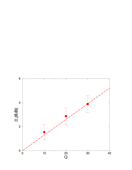
Fig. 2: Absolute value of the correlation function $\widetilde{\Sigma}_{\tau}({\bf 0},{\bf 0})$ as a function of the topological charge $Q$. Notice that the correlator (2.25), which relates directly to the EDM, receives contributions only from topologically non-trivial sectors, as expected. These results were obtained in the quenched approximation, by averaging over the configurations of an ensemble of $130$ pseudo-particles in a volume $V=3.1^{3}\times 4=120$ fm⁴ and quark masses of $m_{q}=0.65~{}\Lambda_{QCD}$.

4 Chiral behavior of the neutron EDM within the IILM

In this Section we derive the qualitative behavior of the expressions (3.39) and (3.40) in the chiral limit by studying the two quantities appearing in the r.h.s. of Eq. (3.36). We will not consider corrections arising from chiral loops.

Let us start with the unquenched case, where the topological susceptibility $\langle Q^{2}\rangle$ vanishes linearly in the quark mass

$$\langle Q^{2}\rangle\propto m~{}.$$ (4.41)

Let us now look at the second factor in the r.h.s. of Eq. (3.36). Writing out the discrete derivative explicitly one has

$$\left(\frac{d}{dQ}\langle\mathcal{O}\rangle\right)_{Q=0}=\frac{\langle\mathcal{O}\rangle_{Q=1}-\langle\mathcal{O}\rangle_{Q=0}}{(Q=1)}=\langle\mathcal{O}\rangle_{Q=1}~{},$$ (4.42)

where we have used the fact that the average of our $CP$ violating operator vanishes in trivial topological sectors ($Q=0$). Writing the average $\langle\mathcal{O}\rangle_{Q}$ explicitly in terms of functional integrals one gets

$$\langle O\rangle_{Q} = \frac{1}{\mathcal{Z}}\int_{(Q)}\mathcal{D}A_{\mu}\prod_{f}\left[m_{f}^{Q}\prod_{\lambda>0}\left(\lambda^{2}+m_{f}^{2}\right)\right]$$ (4.43)

$$\cdot e^{-S_{YM}}~{}\mathrm{Tr}[SS...]~{},$$

where $\mathrm{Tr}[SS...]$ denotes a trace of propagators arising from the explicit integration over the fermionic fields (Wick contractions).

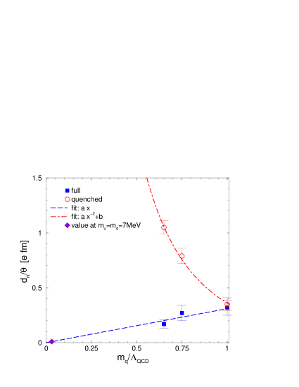
Fig. 3: ILM results obtained at different values of the quark masses with quenched (circles) and unquenched (squares) simulations. The behavior of the unquenched and quenched calculations for small quark masses is consistent with Eqs. (4.49) and (4.50), respectively.

In order to study the chiral behavior of the trace we recall that a quark propagator in the given background can be written as:

$$S(x,y) = \sum_{\lambda}\frac{\psi_{\lambda}(x)\psi_{\lambda}^{\dagger}(y)}{\lambda-im_{f}}~{},$$ (4.44)

$$D{\hskip-6.25958pt}/~{}\psi_{\lambda}(x) = \lambda~{}\psi_{\lambda}(x)~{}.$$ (4.45)

In a topologically non-trivial sector of the instanton vacuum, the Dirac operator has $Q$ exact zero-modes associated to the extra instantons (or anti-instantons) in the ensemble:

$$D{\hskip-6.25958pt}/~{}\psi_{0}^{j}=0~{},\qquad j=1,...,Q~{}.$$ (4.46)

The quark propagator can then be written as:

$$S(x,y) = \sum_{j=1}^{Q}\frac{\psi_{0}^{j}(x)\psi_{0}^{j\dagger}(y)}{-im_{f}}+\sum_{\lambda\neq 0}\frac{\psi_{\lambda}(x)\psi_{\lambda}^{\dagger}(y)}{\lambda-im_{f}}$$ (4.47)

$$\doteq S_{top}(x,y)+S_{non-top}(x,y)~{}.$$

In this expression $S_{top}(x,y)$ is the topological contribution to the propagator arising from the exact zero-modes.

It is important to recall that the Pauli principle implies that at most $N_{f}$ quarks can propagate in the exact zero-mode wave function of an instanton. Thus one has

$$\mathrm{Tr}[SS...]\propto\frac{1}{m^{N_{f}}}~{}.$$ (4.48)

Collecting the results for chiral behavior of all the terms relevant for the EDM, one gets

$$D^{(unq.)}\propto\langle Q^{2}\rangle\cdot\langle\mathcal{O}\rangle_{Q=1}\propto m\cdot m^{N_{f}}\cdot\frac{1}{m^{N_{f}}}\propto m~{}.$$ (4.49)

Hence we conclude that, when the fermionic determinant is included, the neutron EDM vanishes linearly in the quark mass, as it is also expected from other estimates based on chiral perturbation theory (see, e.g., Ref. Crewther ).

When the quenched approximation is adopted, the topological susceptibility $\langle Q^{2}\rangle$ becomes independent of the quark mass, while neglecting the fermionic determinant removes a factor $m^{N_{f}}$ from the numerator of the r.h.s. of Eq. (4.49). Therefore one expects a divergent behavior in the chiral limit of the form

$$D^{(q.)}\propto\frac{1}{m^{N_{f}}}~{}.$$ (4.50)

We stress the fact the mass dependencies given in Eqs. (4.49) and (4.50) do not depend on the particular values of the model parameters which define the ILM. These results rely only on the working assumption that the quantum mixing of the QCD vacuum can be described in terms of isolated tunneling events (instantons). In such a semi-classical limit, the Index Theorem is realized in a very specific way, with $N_{f}$ exact zero-modes associated to each unit of topological charge.

5 Numerical results

We have performed quenched and unquenched numerical simulations in the IILM, assuming two active degenerate flavors. We have used three values of the quark mass $m$, namely $m=0.65,0.75,1.0$, in units of the Pauli-Villars scale parameter $\Lambda_{QCD}=220$ MeV shuryakrev . Correspondingly, we have used three periodic boxes of volume given by $V=(3.1^{3}\times 4),~{}(2.8^{3}\times 4)$ and $(2.4^{3}\times 4)$ fm⁴. The total density of pseudo-particles in these ensembles has been chosen to satisfy $(N_{+}+N_{-})/V=1$ fm^-4.

We have computed the quantities which are needed to determine $D/\overline{\theta}$ through Eqs. (3.39) and (3.40). The neutron mass $M$ and the coupling $Z$ of the interpolating operator have been obtained by extracting the slope and intercept of the logarithm of the two-point function (see the example in Fig. 1). The derivative of (2.25) with respect to $Q$ has been computed by varying by a small amount the number of instantons relative to that of anti-instantons in the box, while keeping the total number of pseudo-particles fixed  (see the example in Fig. 2).

The results of our calculations are summarized in Tables 1-2. From Table 1 we observe that, in case of the quark condensate, the neutron mass and the constant $Z$, quenched and unquenched simulations give almost the same results. This is as expected, since these quantities are not directly related the topological structure of the QCD vacuum. On the contrary, the quantities reported in Table 2 show a much larger sensitivity to the effects of the inclusion of the fermionic determinant. In particular the topological susceptibility $\langle Q^{2}\rangle$ [see Eqs. ( 3.37) and (3.38)] and the EDM $D/\overline{\theta}$ [see Eqs. (3.39) and (3.40)] can differ by a factor of $\simeq 3\div 4$ between the quenched and unquenched simulations with our choice of the quark mass values.

$\stackrel{{\scriptstyle\mbox{V = 56 fm}^{4}}}{{\mbox{m = 1.00 }\Lambda_{QCD}}}$	$|\mathbf{\langle}\overline{\psi}\psi\mathbf{\rangle}|^{1/3}$ [GeV]	$M_{N}$ [GeV]	$Z$ [GeV6]
quenched	0.186	1.42	0.018
unquenched	0.186	1.41	0.017

$\stackrel{{\scriptstyle\mbox{V = 90 fm}^{4}}}{{\mbox{m = 0.75 }\Lambda_{QCD}}}$	$|\mathbf{\langle}\overline{\psi}\psi\mathbf{\rangle}|^{1/3}$ [GeV]	$M_{N}$ [GeV]	$Z$ [GeV6]
quenched	0.199	1.32	0.018
unquenched	0.187	1.30	0.016

$\stackrel{{\scriptstyle\mbox{V = 120 fm}^{4}}}{{\mbox{m = 0.65 }\Lambda_{QCD}}}$	$|\mathbf{\langle}\overline{\psi}\psi\mathbf{\rangle}|^{1/3}$ [GeV]	$M_{N}$ [GeV]	$Z$ [GeV6]
quenched	0.204	1.27	0.018
unquenched	0.199	1.10	0.012

Table 1: Results of quenched and unquenched simulations for the quark condensate $\mathbf{\langle}\overline{\psi}\psi\mathbf{\rangle}^{1/3}$, the neutron mass $M$ and the constant $Z$. The parameter $\Lambda_{QCD}$ is taken at the value $\Lambda_{QCD}=220$ MeV.

$\stackrel{{\scriptstyle\mbox{V = 56 fm}^{4}}}{{\mbox{m = 1.00 }\Lambda_{QCD}}}$	$\langle Q^{2}\rangle$	$|d\widetilde{\Sigma}_{\tau}/dQ|$ [GeV8]	$D/\overline{\theta}$ [e $\cdot$ fm]
quenched	56	0.015	0.35 $\pm 0.06$
unquenched	22	0.025	0.32 $\pm 0.04$

$\stackrel{{\scriptstyle\mbox{V = 90 fm}^{4}}}{{\mbox{m = 0.75 }\Lambda_{QCD}}}$	$\langle Q^{2}\rangle$	$|d\widetilde{\Sigma}_{\tau}/dQ|$ [GeV8]	$D/\overline{\theta}$ [e $\cdot$ fm]
quenched	90	0.043	0.79 $\pm 0.07$
unquenched	32	0.039	0.27 $\pm 0.07$

$\stackrel{{\scriptstyle\mbox{V = 120 fm}^{4}}}{{\mbox{m = 0.65 }\Lambda_{QCD}}}$	$\langle Q^{2}\rangle$	$|d\widetilde{\Sigma}_{\tau}/dQ|$ [GeV8]	$D/\overline{\theta}$ [e $\cdot$ fm]
quenched	120	0.064	1.04 $\pm 0.06$
unquenched	40	0.046	0.17 $\pm 0.04$

Table 2: Results of quenched and unquenched simulations for the topological susceptibility $\langle Q^{2}\rangle$, the quantity $d\widetilde{\Sigma}_{\tau}/dQ$ and the neutron EDM divided by the angle $\overline{\theta}$. The statistical error in the last column is dominated by the uncertainty on the quantity $d\widetilde{\Sigma}_{\tau}/dQ$.

The quenched and unquenched results obtained for the EDM are also shown in Fig. 3 in order to better appreciate the quark mass dependence. The unquenched results appear to be consistent with a linear dependence on $m$ with a zero intercept, as expected from QCD and from the arguments leading to Eq. (4.49). At the same time the quenched results exhibit a sharp increase at low quark masses, consistent with a divergence of the form given by Eq. (4.50) with $N_{f}=2$. Clearly, a quenched calculation of the neutron EDM becomes completely unreliable for $m_{q}\lesssim\Lambda_{QCD}$.

In the quenched approximation, the divergence appearing in the chiral limit makes it impossible to perform the extrapolation toward the physical quark mass value. On the other hand, such an extrapolation is possible in the case of unquenched results. Assuming a linear mass dependence, the IILM prediction for the neutron EDM corresponding to a light quark mass between 4 and 10 MeV is:

$$|{\bf d}_{n}|=(6\div 14)\times 10^{-3}~{}\overline{\theta}~{}(\textrm{e}~{}\cdot~{}\textrm{fm})~{}.$$ (5.51)

6 Conclusions

We have used the Instanton Liquid Model to study the role played by the fermionic determinant in the evaluation of the neutron EDM, which is an observable sensitive to the topological structure of the vacuum. We have analyzed the chiral behavior of such a quantity (up to chiral logs) both in the quenched and unquenched cases. We have found that, when the fermionic determinant is included, the neutron EDM is expected to vanish linearly with the quark mass, whereas in the quenched approximation it should diverge as $1/m^{N_{f}}$ in the chiral limit.

We have performed several model simulations and found that quenched and unquenched calculations give comparable results for the neutron EDM at large quark masses ($\simeq\Lambda_{QCD}$), whereas they strongly differ at lower quark masses. At the lowest value of the quark mass used in our simulations ($m\simeq 130$ MeV) the quenched result is a factor of $\simeq 4$ larger than the unquenched one.

We have obtained the ILM prediction for the neutron EDM by extrapolating the unquenched IILM result to the physical value of the quark mass. The ILM result is roughly a factor $2\div 4$ larger than existing model estimates Baluni ; Crewther .

Our main conclusion is that quenched and unquenched lattice QCD simulations of the neutron EDM as well as of other observables governed by topology might show up similar important differences in the quark mass dependence, near the chiral limit. In particular, our semi-classical analysis suggests that a quenched lattice calculation of the neutron EDM could be affected by a topology-driven divergence, which would make it impossible to perform the extrapolation to the physical value of the quark mass.

We insist on the fact that the qualitative predictions in Eq. (4.49) and (4.50) do not depend on the particular values of the model parameters which define the ILM. They rely only on a semi-classical description of the quantum mixing in the $\theta$-vacuum, in terms of isolated tunneling events. Hence, the observation of a divergence in a quenched lattice calculation of the neutron EDM, would represent a clean, parameter-free signature of instanton-induced dynamics in QCD.

References

- (1) G. ’t Hooft: Phys. Rev. Lett. 37, 8 (1976); Phys. Rev. D14, 3432 (1976).
- (2) P.G. Harris et al.: Phys. Rev. Lett. 82, 904 (1999).
- (3) V. Baluni: Phys. Rev. D19, 2227 (1979).
- (4) R.J. Crewther et al.: Phys. Lett. B88, 123 (1979); errata ibid. B91, 487 (1980).
- (5) S. Aoki et al.: Phys. Rev. Lett. 65, 1092 (1990).
- (6) D. Guadagnoli, V. Lubicz, G. Martinelli and S. Simula: JHEP 0304, 019 (2003). D. Guadagnoli and S. Simula: Nucl. Phys. B670, 264 (2003).
- (7) M. Gockeler et al.: Phys. Lett. B233, 192 (1989).
- (8) A. Ali Khan et al. (CP-PACS collaboration): Phys. Rev. D65, 054505 (2002).
- (9) C.T.H. Davies et al.: Phys. Rev. Lett. 92, 022001 (2004). M. Wingate et al.: Phys. Rev. Lett. 92, 162001 (2004).
- (10) D. Diakonov, Chiral symmetry breaking by instantons, Lectures given at the ”Enrico Fermi” school in Physics, Varenna, June 25-27 1995, hep-ph/9602375.
- (11) T. Schäfer and E.V. Shuryak: Rev. Mod. Phys. 70, 323 (1998).
- (12) M.C. Chu, J.M. Grandy, S. Huang, and J.W. Negele: Phys. Rev. D49, 6039 (1994).
- (13) T.A. DeGrand and A. Hasenfratz: Phys. Rev. D64, 034512 (2001).
- (14) P. Faccioli and T.A. DeGrand: Phys. Rev. Lett. 91, 182001 (2003).
- (15) E.V. Shuryak: Nucl. Phys. B214, 237 (1982).
- (16) P. Faccioli: hep-ph/0312019, Phys. Rev. C in press.
- (17) E.V. Shuryak and J.J. Verbaarschot: Phys. Rev. D52, 295 (1995).
- (18) P. Faccioli: hep-ph/0404137.
- (19) T. Schäfer and E.V. Shuryak: Phys. Rev. D53, 6522 (1996).
- (20) D. Diakonov and V. Petrov: Nucl. Phys. B245, 259 (1984).
- (21) J.W. Negele: Nucl. Phys. Proc. Suppl. 73, 92 (1999).
- (22) D.I. Diakonov, M.V. Polyakov and C. Weiss: Nucl. Phys. B461, 539 (1996).