A nonperturbative calculation of the electron’s magnetic moment

Abstract

In principle, the complete spectrum and bound-state wave functions of a quantum field theory can be determined by finding the eigenvalues and eigensolutions of its light-cone Hamiltonian. One of the challenges in obtaining nonperturbative solutions for gauge theories such as QCD using light-cone Hamiltonian methods is to renormalize the theory while preserving Lorentz symmetries and gauge invariance. For example, the truncation of the light-cone Fock space leads to uncompensated ultraviolet divergences. We present two methods for consistently regularizing light-cone-quantized gauge theories in Feynman and light-cone gauges: (1) the introduction of a spectrum of Pauli–Villars fields which produces a finite theory while preserving Lorentz invariance; (2) the augmentation of the gauge-theory Lagrangian with higher derivatives. In the latter case, which is applicable to light-cone gauge ($A^{+}=0$), the $A^{-}$ component of the gauge field is maintained as an independent degree of freedom rather than a constraint. Finite-mass Pauli–Villars regulators can also be used to compensate for neglected higher Fock states. As a test case, we apply these regularization procedures to an approximate nonperturbative computation of the anomalous magnetic moment of the electron in QED as a first attempt to meet Feynman’s famous challenge.

and

1 Introduction

The gyromagnetic ratio of the electron $g_{e^{-}}=2.0023193043768(86)$, the ratio of the spin precession frequency to the Larmor precession frequency in a static magnetic field, is an intrinsic property of an individual lepton. It is now known experimentally to $12$ significant figures [1] – the most precisely known fundamental physical parameter. The anomalous moment $a_{e}={g_{e}-2\over 2}$, the deviation of the gyromagnetic ratio from Dirac’s value $g_{e}=2$ due to quantum fluctuations, has now been evaluated through order ${\alpha}^{4}$ in perturbative quantum electrodynamics [2, 3].

At the 12th Solvay Conference, Feynman presented a challenge [4]: “Is there any method of computing the anomalous moment of the electron which, on first approximation, gives a fair approximation to the $\alpha$ term and a crude one to $\alpha^{2}$; and when improved, increases the accuracy of the $\alpha^{2}$ term, yielding a rough estimate to $\alpha^{3}$ and beyond.” An interesting attempt to answer Feynman’s challenge using sidewise dispersion relations was pioneered by Drell and Pagels [5], but it is difficult to make this method systematic.

The anomalous moment of a spin-half particle can be evaluated without approximation from the overlap of its light-cone Fock-state wave functions. The overlap of the two-particle one-fermion–one-boson light-cone Fock state $|f\gamma>$ yields Schwinger’s contribution [6] $a_{e}={\alpha\over 2\pi}$. The light-cone wave functions with $n\geq 2$ QED quanta contribute to $a_{e}$ beginning at order $\alpha^{n-1}$ as well as higher orders. Thus a systematic evaluation of the lepton’s Fock-state wave functions as an expansion in Fock number rather than perturbation theory would provide a physically appealing answer to Feynman’s challenge [7].

In principle the complete spectrum of a quantum field theory can be determined by finding the eigenvalues of the light-cone Hamiltonian [8]. The Fock-state expansion of the eigensolutions at fixed light-cone time $\tau=x^{+}=x^{0}+x^{z}$ provides a frame-independent wave-function description of the elementary and composite states in terms of the quanta of the free Hamiltonian. The discretized light-cone quantization (DLCQ) method utilizes periodic boundary conditions to truncate the size of the Fock-state expansion while preserving boost invariance. This method has been successfully applied to a large variety of gauge theories and supersymmetric theories in $1+1$ and $2+1$ dimensions.

An essential problem in applying light-cone Fock-state methods to renormalizable gauge theory is to regularize the calculations in such a way as to preserve Lorentz and gauge invariance, or at least preserve them well enough to allow an effective renormalization to be performed. Since the method of regularization must also allow for efficient calculations to be performed, the problem presents a challenge.

We have recently performed nonperturbative calculations using the generalized Pauli–Villars (PV) method as an ultraviolet regulator of (3+1)-dimensional quantum field theories. We include a sufficient number of PV fields in the Lagrangian to ensure that perturbation theory is finite. This method explicitly preserves Lorentz invariance; in some cases, such as QED, it effectively preserves gauge invariance. In a case where it breaks gauge invariance, such as QCD, we have to add counterterms. The PV regularization can produce a finite theory which preserves Lorentz and gauge symmetries. However, if we do not have the exact solution, we must develop approximate methods. Our approximation involves truncating the Fock space. The truncation will break all of the symmetries. However, the usefulness of the truncated answer is a question of accuracy rather than an issue of symmetry breaking. With regulators in place we presume that there is an exact solution which preserves all symmetries including gauge invariance, and if our approximate solution is close to the exact one, even if the small difference is in such a direction as to maximally violate the symmetries, it is still a small difference. Of course, the inclusion of negative-metric fields in the Lagrangian will also violate unitarity. We shall have more to say about this issue below.

The generalized PV method has been applied successfully to Yukawa-like theories [9, 10, 11, 12, 13] where there are no infrared divergences and no need to protect gauge symmetry. An important conclusion of these studies is that past some threshold (which depends on the values of the coupling constant and the values of the PV masses), there is always a rapid drop off of the projection of the eigensolution wave function onto higher Fock sectors, in contrast to the equal-time Fock-space expansion. This provides a strong motivation for the light-cone representation as a viable approximant to nonperturbative theory.

In this paper we will test the convergence of the PV-regulated light-cone Fock-state expansion for (3+1)-dimensional gauge theory by applying it to a nonperturbative calculation of the electron anomalous moment in QED. In some ways this application to QED is not an ideal test of these nonperturbative methods: the physical electron is a very perturbative object. We do not expect to do better, or even as well as perturbation theory. However, that is not our objective; we simply want to verify that an approximate nonperturbative solution for the electron’s magnetic moment is an approximation to QED. Somewhat related work, from a strictly perturbative point of view, can be found in [14].

Careful studies have also shown [15, 16] that the perturbative series obtained from particular combinations of PV fields and higher derivative regulators give the same result as standard perturbation series regulated with dimensional regularization. These studies not only included Yukawa theory, but also non-Abelian gauge theory. In Section 4, we shall apply this method of regularization, together with a Fock-space truncation to the calculation of the electron magnetic moment. This is the first application of this regularization to a nonperturbative problem.

We find that there are three problems which must be solved in order to produce a useful calculation of the electron’s magnetic moment: the problem of uncanceled divergences, the problem of maintaining gauge invariance, and the problem of new singularities. We believe that we have found effective solutions to these problems, at least for the present calculations. The problem of uncanceled divergences occurs anytime we truncate the Fock space. For example, if we truncate the physical electron’s Fock space to include only the subspace of one fermion and one photon, calculate the wave function nonperturbatively, and use that wave function to calculate the moment, we obtain a result of the form:

$$a_{e}={\alpha\times{\rm[finite\;quantity]}\over 1+\alpha\times{\rm[finite\;quantity]}+\alpha\times{\rm[finite\;quantity]}\log{\mu_{1}\over m^{2}_{e}}},$$ (1)

where $\mu_{1}$ is the PV photon mass. If we let $\mu_{1}$ become infinite, we will obtain a zero anomalous moment.

The origin of the uncanceled divergence in Eq. (1) can be seen by examining the two-loop contributions to the electron moment in perturbation theory. The relevant double-ladder Feynman diagrams are shown in Fig. 1.

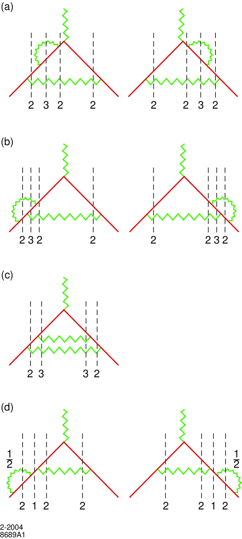
Figure 1: Light-cone time-ordered contributions to the lepton form factors, corresponding to the order-$\alpha^{2}$ ladder Feynman diagram in perturbative QED. The vertical dashed lines mark intermediate states with the indicated number of constituents. For amplitudes associated with diagrams in (d), with loops on the external legs, a factor of 1/2 is applied.

The Dirac $F_{1}(q^{2})$ and Pauli $F_{2}(q^{2})$ form factors correspond to $S_{z}=\pm S_{z}^{\prime}$ matrix elements, respectively. (The $q^{+}=0$, $q^{2}_{\perp}=Q^{2}=-q^{2}$ frame is assumed.) Fock states with particle number 1,2,3 contribute as indicated in the figure. Only time orderings with positive $k^{+}$ appear in light-cone quantization. The Ward identity $Z_{1}=Z_{2}$ guarantees the cancellation of the divergences from wave function and vertex renormalization subgraphs. However, if the three-particle Fock state $|f\gamma\gamma>$ is excluded by the truncation of the Fock space, $F_{2}$ is ultraviolet (UV) divergent since the vertex correction shown in amplitude (c) is missing. The divergent contribution to the lepton anomalous moment $a_{\ell}=F_{2}(0)$ is the source of the UV divergence in the denominator of Eq. (1) due to Fock-space truncation. Of course, $F_{1}$ remains UV finite. The divergence in Eq. (1) does not happen in perturbation theory; since the numerator is already of order $\alpha$, we would use only the 1 from the denominator. At order $\alpha^{2}$ there would be new terms in the numerator which would cancel the divergent terms in the denominator of Eq. (1).

The above discussion illustrates the problem of uncanceled divergences. While we could find ways of allowing the bare mass and the coupling constant to depend on the PV masses to give a finite expression, the results would not look anything like the results from perturbation theory, since in QED the coupling is renormalized only by vacuum polarization. In addition, the results would not make sense physically. Our resolution of this difficulty is to keep the PV masses finite. The motivation is as follows: If the limit of infinite PV masses would give a useful answer in the case where we do not truncate the Fock space (so we have no uncanceled divergences), then there must be some finite value of the PV masses that would also give a useful answer. The question is whether we can use a sufficiently large value. To answer that question we must consider that there are two types of error associated with the values of the PV masses. The first type of error results in having these masses too small; then our wave function will contain too much of the negative-normed states, unitarity will be badly violated, and in the worst case we might get negative probabilities. We can roughly estimate the magnitude of that type of error as

$$E_{1}={M^{2}_{0}/M^{2}_{1}},$$ (2)

where $M_{0}$ is the physical mass scale and $M_{1}$ is the PV mass scale. The other type of error results when the PV masses are too large; in that case the true wave function will project significantly onto the parts of the representation space excluded by the truncation. We can roughly estimate the magnitude of that type of error as

$$E_{2}={\langle\Phi_{+}^{\prime}|\Phi_{+}^{\prime}\rangle\over\langle\Phi_{+}|\Phi_{+}\rangle},$$ (3)

where $|\Phi_{+}^{\prime}\rangle$ is the projection of the wave function onto the excluded sectors. In practice, the projection onto the first excluded Fock sector can be estimated perturbatively using the projection of $P^{-}$ onto the higher sectors as the perturbing operator. Without additional information, the best that we can do is to set $E_{1}$ equal to the perturbative estimate of $E_{2}$. Below, we will apply this procedure to the calculation of the magnetic moment done in this paper. In general, if, at our estimated optimum value for the PV mass scale both types of error are small, we can do a useful calculation; otherwise, we cannot do a useful calculation without expanding the part of the representation space that we include in our calculation.

The main reason for believing that we can do a useful calculation in spite of the problem of uncanceled divergences is the lesson from the earlier studies mentioned above: the observed rapid drop off of the projection of the wave function onto higher Fock sectors. Just where this rapid drop off occurs depends on the theory, the coupling constant, and the values of the PV masses. At weak coupling and relatively light PV masses, only the lowest Fock sectors are significantly populated. At stronger coupling or heavier PV masses, more Fock sectors will be populated; but eventually the projection onto higher sectors will fall rapidly. The rapid drop off of the projection of the wave function onto sufficiently high Fock sectors is the most important reason why we do our calculations in the light-cone representation. For any practical calculation in a realistic theory, we have to truncate the space, and we must have a framework in which that procedure can lead to a useful calculation. The rapid drop off in the projection of the wave function will not happen in the equal-time representation, mostly due to the complexity of the vacuum in that representation.

These features can be explicitly demonstrated by setting the PV masses equal to the physical masses. In that case the theory becomes exactly solvable [12]. The spectrum is the free spectrum, and the theory is not useful for describing real physical processes due to the strong presence of the negative-norm states in physical wave functions; however, it still illustrates the points we have been trying to make. In the equal-mass case, the physical vacuum is the bare light-cone vacuum, while it is a very complicated state in the equal-time representation; the physical wave functions project onto a finite number of Fock sectors in the light-cone representation but onto an infinite number of sectors in the equal-time representation.

As the PV masses become larger than the physical masses, the light-cone wave functions project onto more of the representation space. This effect is increased as the coupling constant becomes larger. However, the wave functions remain much simpler than in the equal-time representation, and, to the extent we can do the calculations, there is always a point of rapid drop off of the projection onto higher Fock sectors. Due to this rapid drop off, we expect to find a PV mass scale such that the error in the calculated value for a given observable from the presence of negative-norm states and the error from truncation can both be made arbitrarily small. Therefore, we believe the requirement to keep the value of the PV masses finite does not impose a limit on the accuracy which could, in principle, be achieved. In practice, the size of the representation space may be too large for presently available computing facilities. Furthermore, for the method to be useful in practice, there must not only be a value of the PV mass for which both types of errors are small, but there must be a wide range of such values since the optimum value for the PV mass can only be rather crudely estimated. A principal objective of the present work is to test these ideas on a physically realistic problem to which we know the answer.

The problem of maintaining gauge invariance turns out to be nontrivial and quite instructive. In the next section we consider the following procedure: we take the light-cone evolution operator $P^{-}$ for QED in light-cone gauge $A^{+}=0$ as constructed, for example, in Refs. [17] and regulate it with PV fields. We looked at several cases: PV photons alone, PV fermions alone, and a combination of both. This procedure does not lead to a viable nonperturbative formalism for the electron magnetic moment; furthermore, it does not lead to a correct calculation of the electron self-energy, even at order $\alpha.$ The problem can be traced to a failure to maintain gauge invariance. The breakdown of the straightforward implementation of the PV method in light-cone gauge shows that the successful construction of the nonperturbative theory is nontrivial.

In Section 3 we perform the calculation in Feynman gauge with one PV photon and one PV fermion; this leads to a consistent formulation for the nonperturbative calculation of the electron moment in QED. In Section 4 we perform the calculation in light-cone gauge, but use the more sophisticated method of regulation proposed in [16]. We show that this method provides a successful formulation of the nonperturbative electron moment problem in light-cone gauge with a result very similar to that in Feynman gauge.

In Sections 3 and 4 we face the problem of new singularities. We have to do integrals with denominators of the form $(-M^{2}x(1-x)+m^{2}x+\mu^{2}(1-x)+k_{\perp}^{2})$, where $M$ is the physical electron mass, $m$ is the bare electron mass, and $\mu$ is the photon mass. When the bare mass is less than the physical mass, as is the case in QED, there can be a zero in this denominator. In perturbation theory the expansion is about $M=m$, and the denominator cannot vanish as long as the photon is given a small nonzero mass. The standard techniques in perturbation theory thus avoid this singularity. We find that when the zero is a simple pole, the principal-value prescription is correct. However, in the wave function normalization the denominator is squared, so there is a double pole, and we must give it a meaning. We propose the following prescription:

$$\int dy\;dk_{\perp}^{2}\;{f(y,k_{\perp}^{2})\over[m^{2}y+\mu_{0}^{2}(1-y)-M^{2}y(1-y)+k_{\perp}^{2}]^{2}}$$

$$\equiv\lim_{\epsilon\rightarrow 0}{1\over 2\epsilon}\int dy\int dk_{\perp}^{2}f(y,k_{\perp}^{2})\Bigg{[}{1\over[m^{2}y+\mu_{0}^{2}(1-y)-M^{2}y(1-y)+k_{\perp}^{2}-\epsilon]}$$

$$-{1\over[m^{2}y+\mu_{0}^{2}(1-y)-M^{2}y(1-y)+k_{\perp}^{2}+\epsilon]}\Bigg{]},$$ (4)

where simple poles are prescribed as principal values.

This prescription has the interesting consequence that the wave function normalization is infrared finite whereas it is infrared divergent in perturbation theory. Given this prescription, the true singularity occurs at $M=m+\mu$; in perturbation theory, with $M=m$, this is at $\mu=0$, which is the infrared singularity and the reason that the photon mass cannot be taken all the way to zero in perturbation theory. For the nonperturbative calculation, the physical photon mass can be taken to zero since $M\neq m$. The basic requirement of these prescriptions is that they preserve the Ward identities. We anticipate using this prescription for QCD where the basic requirement will be the preservation of the Ward–Takahashi identities. We have not shown that the prescription preserves the Ward identities in QED, but it does lead to a successful calculation in the present case.

A different approach to this same dressed-electron problem has been taken by Karmanov, Mathiot, and Smirnov [18]. They use a covariant form of light-cone quantization without Pauli–Villars regularization. Their Hamiltonian then contains instantaneous fermion interactions, and, in Feynman gauge, the infinite number of terms generated by inversion of the covariant derivative. The problem of uncancelled divergences is avoided by application of sector-dependent renormalization [19]. They must construct counterterms explicitly. However, they truncate in a Fock basis where the constituent electron has the same mass as the dressed electron, bringing their calculation closer to perturbation theory; in fact, they find that any signifant difference with perturbation theory will not appear until the basis is expanded to include higher Fock states. Also, they do not calculate the anomalous moment.

2 Trouble in Light-Cone Gauge

In this and the next section the notation that we use for light-cone coordinates is

$$x^{\pm}=x^{0}\pm x^{3}\,,\;\;\vec{x}_{\perp}=(x^{1},x^{2}).$$ (5)

The time coordinate is $x^{+}$, and the dot product of two four-vectors is

$$p\cdot x=\frac{1}{2}(p^{+}x^{-}+p^{-}x^{+})-\vec{p}_{\perp}\cdot\vec{x}_{\perp}.$$ (6)

The momentum component conjugate to $x^{-}$ is $p^{+}$, and the light-cone energy is $p^{-}$. Light-cone three-vectors are identified by underscores, such as

$$\underline{p}=(p^{+},\vec{p}_{\perp}).$$ (7)

We use the following choice for the $\gamma$ matrices

$$\gamma^{0}=\left(\begin{array}[]{cc}I&0\\ 0&-I\end{array}\right),\qquad \gamma^{+}=\left(\begin{array}[]{cc}I&\sigma_{3}\\ -\sigma_{3}&-I\end{array}\right),$$ (12)

$$\gamma^{-}=\left(\begin{array}[]{cc}I&-\sigma_{3}\\ \sigma_{3}&-I\end{array}\right),\qquad \gamma^{k}=i\left(\begin{array}[]{cc}0&\sigma_{k}\\ -\sigma_{k}&0\end{array}\right).$$ (17)

For additional details, see Appendix A of Ref. [9].

We use the standard $P^{-}$ for light-cone quantized QED in light-cone gauge [17] with modifications due to the inclusion of the PV fields. We should remark, however, that with the inclusion of any number of PV Fermi fields, the four-point interactions which would take a state of one electron and one photon to another state of one electron and one photon are missing from $P^{-}$; that such terms are not included below is not an omission; the calculation is complete in our chosen subspace. We truncate the Fock space to the one-fermion sector plus the one-fermion, one-photon sector. We then solve the eigenvalue problem

$$P^{+}P^{-}|s\rangle=M^{2}|s\rangle,$$ (18)

where the total $\vec{P}_{\perp}$ of the state is taken equal to 0. As always with a Tamm-Dancoff truncation, we can solve for the wave function in the highest Fock sector (one fermion plus one photon) by hand and obtain an equation in the one-fermion sector.

We have regulated the theory in several ways. We shall describe one particular choice in some detail: We use three PV Fermi fields with flavor-changing currents. The flavor-changing currents break gauge invariance, and thus we might expect to require counterterms to correct for that. Nevertheless, we will proceed with the calculation without counterterms. That will allow us to study a case where a proper respect for gauge invariance is not maintained. Also, as we shall argue below, the source of the breaking of gauge invariance is much deeper than that due to the flavor-changing currents.

For the Lagrangian we take

$$-{1\over 4}F^{\mu\nu}F_{\mu\nu}+\sum_{i=0}^{3}{1\over\nu_{i}}\bar{\psi_{i}}^{\prime}(i\gamma^{\mu}\partial_{\mu}-m_{i})\psi_{i}^{\prime}-e\bar{\psi}^{\prime}\gamma^{\mu}\psi^{\prime}A_{\mu},$$ (19)

where

$$\psi^{\prime}=\sum_{i=0}^{3}\psi_{i}^{\prime},\quad\sum_{i=0}^{3}\nu_{i}=0,\quad\sum_{i=0}^{3}\nu_{i}m_{i}=0,\quad\sum_{i=0}^{3}\nu_{i}m_{i}^{2}=0.$$ (20)

A particular realization of these PV conditions is

$$\{\nu_{i}\}=\{1;3;-1;-3\},\quad\{m_{i}\}=\{m_{0};-m_{0}+2m_{3};-2m_{0}+3m_{3};m_{3}\}.$$ (21)

With this choice it is convenient to define

$$\psi_{0}=\psi_{0}^{\prime},\quad\psi_{1}=\sqrt{3}\psi_{1}^{\prime},\quad\psi_{2}=\psi_{2}^{\prime},\quad\psi_{3}=\sqrt{3}\psi_{3}^{\prime},$$ (22)

so that the $\psi$ fields are canonically normalized (except for the minus signs for $\psi_{2}$ and $\psi_{3}$). The coupling to the $A$ field is

$$e\bar{\psi}^{\prime}\gamma^{\mu}\psi^{\prime}A_{\mu}=\sum_{ij}g_{ij}\bar{\psi}_{i}\gamma^{\mu}\psi_{j}A_{\mu},$$ (23)

where

$$g_{00} = g_{02}=g_{22}=e,\quad g_{01}=g_{03}=g_{12}=g_{23}=\sqrt{3}e,$$ (24)

$$g_{11} = g_{13}=g_{33}=3e,$$

and $g_{ij}=g_{ji}$.

We use the mode expansions

$$\psi_{i+}(\underline{x})={1\over\sqrt{16\pi^{3}}}\sum_{s}\int d\underline{k}\;\chi_{s}\;\Bigl{[}b_{s}(i,\underline{k})e^{-i\underline{k}\cdot\underline{x}}+d^{\dagger}_{-s}(i,\underline{k})e^{+i\underline{k}\cdot\underline{x}}\Bigr{]},$$ (25)

$$A^{i}(\underline{x})={1\over\sqrt{16\pi^{3}}}\sum_{\lambda}\int d\underline{k}\;\;{1\over\sqrt{k^{+}}}\Bigl{[}a_{\lambda}(\underline{k})\epsilon^{i}(\lambda)e^{-i\underline{k}\cdot\underline{x}}+a_{\lambda}^{\dagger}(\underline{k}){\epsilon^{i}(\lambda)}^{*}e^{+i\underline{k}\cdot\underline{x}}\Bigr{]},$$ (26)

where the polarization states are

$$\chi_{+{1\over 2}}={1\over\sqrt{2}}\left(\matrix{1\cr 0\cr 1\cr 0\cr}\right),\qquad\qquad\chi_{-{1\over 2}}={1\over\sqrt{2}}\left(\matrix{0\cr 1\cr 0\cr-1\cr}\right),$$ (27)

$${\epsilon}_{\perp,+1}\equiv{-1\over\sqrt{2}}(1,i),\qquad\qquad{\epsilon}_{\perp,-1}\equiv{1\over\sqrt{2}}(1,-i).$$ (28)

The vertex functions can be computed from $P^{-}$ as

$$V_{ij}={\epsilon_{ij}\over\sqrt{16\pi^{3}}}{1\over\sqrt{1-x}}{1\over x(1-x)}(k_{x}-ik_{y}),$$ (29)

$$W_{ij}={\epsilon_{ij}\over\sqrt{16\pi^{3}}}{1\over\sqrt{1-x}}{1\over(1-x)}(-k_{x}-ik_{y}),$$ (30)

$$U_{ij}={\epsilon_{ij}\over\sqrt{16\pi^{3}}}{1\over\sqrt{1-x}}(-m_{i}+{m_{j}\over x}),$$ (31)

$$\tilde{U}_{ji}={\epsilon_{ji}\over\sqrt{16\pi^{3}}}{1\over\sqrt{1-x}}(-m_{i}+{m_{j}\over x}),$$ (32)

where

$$\epsilon_{ij}\equiv\cases{g_{ij},&if $i=0,1$;\cr-g_{ij},&if $i=2,3$.\cr}$$ (33)

We expand the eigenstate as

$$|s>= \sum_{i=0}^{3}z_{i}b_{+}^{\dagger}(i,\underline{P})|0>+\sum_{i=0}^{3}\int d\underline{k}f(i,x,\vec{k}_{\perp})b_{+}^{\dagger}(i,\underline{k})a_{+}^{\dagger}(\underline{P}-\underline{k})|0>$$

$$+ \sum_{i=0}^{3}\sum_{s=\{-,+\}}\int d\underline{k}g_{s}(i,x,\vec{k}_{\perp})b_{s}^{\dagger}(i,\underline{k})a_{-s}^{\dagger}(\underline{P}-\underline{k})|0>.$$ (34)

We will take the wave function normalization $z_{0}$ to be 1 for the moment and calculate it later. From $P^{+}P^{-}|s>=m_{e}^{2}|s>$ we find immediately (in units where $m_{e}$ is taken to 1):

$$f(i,x,\vec{k}_{\perp})={\sum_{j=0}^{3}z_{j}V_{ji}(x,\vec{k}_{\perp})\over 1-{m_{i}^{2}+k_{\perp}^{2}\over x}-{\mu^{2}+k_{\perp}^{2}\over 1-x}},$$ (35)

$$g_{+}(i,x,\vec{k}_{\perp})={\sum_{j=0}^{3}z_{j}W_{ji}(x,\vec{k}_{\perp})\over 1-{m_{i}^{2}+k_{\perp}^{2}\over x}-{\mu^{2}+k_{\perp}^{2}\over 1-x}},$$ (36)

$$g_{-}(i,x,\vec{k}_{\perp})={\sum_{j=0}^{3}z_{j}U_{ji}(x,\vec{k}_{\perp})\over 1-{m_{i}^{2}+k_{\perp}^{2}\over x}-{\mu^{2}+k_{\perp}^{2}\over 1-x}}.$$ (37)

From all this we derive the four nonlinear equations

$$z_{i}m_{i}^{2}+ \sum_{j=0}^{3}\int dxd^{2}k_{\perp}{V_{ji}^{*}(x,\vec{k}_{\perp})\sum_{l=0}^{3}z_{l}V_{lj}(x,\vec{k}_{\perp})\over 1-{m_{j}^{2}+k_{\perp}^{2}\over x}-{\mu^{2}+k_{\perp}^{2}\over 1-x}}$$

$$+ \sum_{j=0}^{3}\int dxd^{2}k_{\perp}{W_{ji}^{*}(x,\vec{k}_{\perp})\sum_{l=0}^{3}z_{l}W_{lj}(x,\vec{k}_{\perp})\over 1-{m_{j}^{2}+k_{\perp}^{2}\over x}-{\mu^{2}+k_{\perp}^{2}\over 1-x}}$$

$$+ \sum_{j=0}^{3}\int dxd^{2}k_{\perp}{\tilde{U}_{ji}^{*}(x,k_{\perp})\sum_{l=0}^{3}z_{l}U_{lj}(x,k_{\perp})\over 1-{m_{j}^{2}+k_{\perp}^{2}\over x}-{\mu^{2}+k_{\perp}^{2}\over 1-x}}=z_{i}.$$ (38)

These can be written in terms of the three integrals:

$$J=\int dxdz\sum_{i=0}^{3}{1\over x}{({1+x^{2}\over(1-x)^{2}}z+m_{i}^{2})\nu_{i}\over x(1-x)-m_{i}^{2}(1-x)-\mu^{2}x-z},$$ (39)

$$I_{1}=\int dxdz\sum_{i=0}^{3}{m_{i}\nu_{i}\over x(1-x)-m_{i}^{2}(1-x)-\mu^{2}x-z},$$ (40)

$$I_{0}=\int dxdz\sum_{i=0}^{3}{x\nu_{i}\over x(1-x)-m_{i}^{2}(1-x)-\mu^{2}x-z},$$ (41)

where $z=k^{2}_{\perp}.$ The nonlinear equations become

$$z_{i}m_{i}^{2}+{e^{2}\over 16\pi^{2}}J\sum_{j=0}^{3}\epsilon_{ji}z_{j}-{e^{2}\over 16\pi^{2}}I_{1}\sum_{j=0}^{3}\epsilon_{ji}z_{j}(m_{i}+m_{j})$$ (42)

$$+{e^{2}\over 16\pi^{2}}I_{0}\sum_{j=0}^{3}\epsilon_{ji}z_{j}m_{i}m_{j}=z_{i}.$$

While these equations are complicated, they can be simplified by the observation that, for the parameter values of interest, $J$ is very much larger than $I_{0}$ and $I_{1}$. Also, for those parameter values, $z_{1}$, $z_{2}$, and $z_{3}$ are small compared to one, and a solution sufficiently accurate for our needs is given by the simple expression

$$m_{0}^{2}=1-\frac{\alpha}{4\pi}J.$$ (43)

We can use the wave function to calculate the anomalous magnetic moment using the formalism of Brodsky and Drell [20]. The contribution from the physical field is much larger that the contributions from the PV fields, so we have

$$a_{e}={\alpha\over\pi}z_{0}^{2}\int dx{m_{1}x^{2}(1-x)\over m_{1}^{2}x+\mu^{2}(1-x)-x(1-x)},$$ (44)

where $z_{0}$ is determined by wave function normalization:

$$1/z_{0}^{2} = 1+z_{1}^{2}-z_{2}^{2}-z_{3}^{2}$$ (45)

$$+ \int dxd^{2}k_{\perp}(|f(0,x,\vec{k}_{\perp})|^{2}+|f(1,x,\vec{k}_{\perp})|^{2}-|f(2,x,\vec{k}_{\perp})|^{2}-|f(3,x,\vec{k}_{\perp})|^{2})$$

$$+ (|g_{+}(0,x,\vec{k}_{\perp})|^{2}+|g_{+}(1,x,\vec{k}_{\perp})|^{2}-|g_{+}(2,x,\vec{k}_{\perp})|^{2}-|g_{+}(3,x,\vec{k}_{\perp})|^{2})$$

$$+ (|g_{-}(0,x,\vec{k}_{\perp})|^{2}+|g_{-}(1,x,\vec{k}_{\perp})|^{2}-|g_{-}(2,x,\vec{k}_{\perp})|^{2}-|g_{-}(3,x,\vec{k}_{\perp})|^{2}).$$

We find

$$a_{e}={\alpha\over 2\pi}z_{0}^{2}({1\over 2}+\frac{\alpha}{4\pi}J(1+\frac{\alpha}{4\pi}J)\ln({4\pi\over\alpha J}-1)-\frac{\alpha}{4\pi}J).$$ (46)

We can now state the problem with this calculation: $J$ has a very strong dependence on $m_{3}$ (the PV mass scale). That, in turn, gives our estimate of the anomalous magnetic moment a very strong dependence on $m_{3}$. If we use units of ${\alpha\over 2\pi}$, so that the correct value is near one, then we find that, even with a value for the photon mass as large as 0.5 electron masses, when $m_{3}$ changes from 3 times the electron mass to 7 times the electron mass, $a_{e}$ changes from 1.2 to -1.2. If we use a smaller value for the photon mass, which we would surely have to do to get useful results, the dependence is even stronger. Since we cannot hope to estimate the optimum value for the PV mass scale even to within this range, the present calculation is clearly useless. The problem is clearly the loss of gauge invariance; gauge invariance should prevent such strong behavior. One might reasonably think that the problem is the flavor-changing currents we have included in the calculation, but we shall now argue that the worst breaking of gauge invariance has a more fundamental source. We shall return to the breaking due to flavor-changing currents in the next section.

We note that if we keep only the physical field and set $M=m_{0}=m$, the function which appears in our nonlinear equations is just the (unregulated) one-loop fermion self-energy

$$\frac{\alpha}{4\pi}\left(J-2I_{1}+I_{0}\right)=\frac{\alpha}{4\pi}\int dxdz{1\over x}{{1+x^{2}\over(1-x)^{2}}z+m^{2}(1-x)^{2}\over m^{2}x(1-x)-m^{2}(1-x)-\mu^{2}x-z}.$$ (47)

Therefore, a very useful point of comparison is the evaluation of the fermion self-energy calculated in the paper by Brodsky, Roskies and Suaya [21], hereafter referenced as BRS. They evaluated all the graphs needed to calculate the electron’s magnetic moment in perturbation theory through order $\alpha^{2}$. Included in their calculations is the one-loop electron self-energy. They did not use light-cone quantization but wrote down time-ordered perturbation theory in the equal-time representation and then boosted to the infinite momentum frame. They worked in Feynman gauge, but the electron self-energy should be gauge invariant. They give the self-energy as the sum of two separate pieces, $m_{a}$ and $m_{b}$; $m_{b}$ results from boosting the z-graph while $m_{a}$ comes from the other time ordering. They obtain in our notation (see Eqs. (3.40) and (3.41) of BRS)

$$m_{a}={e^{2}\over 16\pi^{2}}\int dxdz{1\over x}{z+m^{2}(1-4x-x^{2})\over m^{2}x(1-x)-m^{2}(1-x)-\mu^{2}x-z},$$ (48)

$$m_{b}=-{e^{2}\over 16\pi^{2}}\int dz\ln(\mu^{2}+z).$$ (49)

BRS show that if the theory is regulated with the inclusion of two PV photons, the sum of $m_{a}$ and $m_{b}$ is equal to the usual Feynman one-loop self-energy in QED, regulated in the same way. Notice that $m_{b}$ implements the requirement of chiral symmetry: the shift in the bare mass is zero if the bare mass is zero, that is, $\delta m_{b}=-\delta m_{a}\bigm{|}_{m=0}$. Terms such as $m_{b}$ are often missed in light-cone quantization. That fact has been noticed at least as far back as the work of Chang and Yan [22]. Those authors suggest that the problem can be solved by including an extra PV field and using it to implement the chiral symmetry condition; that is a technique we have used in the past [9]. Since $m_{b}$ does not depend on the mass, inclusion of PV fermi fields will also solve the problem. That possibility was noticed by BRS, and we shall use this method in the next sections. Therefore without PV fermi fields we might not expect to get the sum of $m_{a}$ and $m_{b}$ correctly, but we should expect to at least reproduce $m_{a}$. We do not have to get the same integrand, but we should get the same result after integration if the regulation preserves covariance. However, if we use two PV photons, or three PV photons with the third field used to eliminate $m_{b}$, we do not obtain the correct result for $m_{a}.$

We can gain some further insight into what is going on by observing that, in Feynman methods, the light-cone gauge is obtained from Feynman gauge by the replacement

$$g^{\mu\nu}\rightarrow g^{\mu\nu}-{n_{\mu}k_{\nu}+n_{\nu}k_{\mu}\over n\cdot k}.$$ (50)

From that replacement there is no obvious source for the double pole at $x=1$ that we see in our light-cone calculation. The explanation is that, in some formal sense without worrying about regulation, light-cone quantization accomplishes the replacement by writing

$$g^{\mu\nu}\rightarrow g^{\mu\nu}-{n_{\mu}k_{\nu}+n_{\nu}k_{\mu}\over n\cdot k}+{k^{2}n^{\mu}n^{\nu}\over(n\cdot k)^{2}}-{k^{2}n^{\mu}n^{\nu}\over(n\cdot k)^{2}}.$$ (51)

The first three terms correspond to the usual three-point interactions that one obtains by usual light-cone quantization as given, for instance, in [17]. The last term is given by the so called “instantaneous” (four-point) interactions which result from solving the constraint equation for the photon. In at least some cases, for tree level processes the required cancellations actually occur, and results equivalent to the equal-time formulation are obtained. However, here, at one loop, the cancellations are not working correctly, and we can see why as follows: If we write down the Feynman integral whose numerator is

$$-{k^{2}n^{\mu}n^{\nu}\over(n\cdot k)^{2}},$$ (52)

regulate the calculation with two PV photons, and perform the $k^{-}$ integral, we get an amplitude which cannot be obtained from a four-point interaction

$$2\int dxdz{1\over x}{z({1\over 1-x}-{1\over(1-x)^{2}})-m^{2}x\over m^{2}x(1-x)-m^{2}(1-x)-\mu^{2}x-z}.$$ (53)

When this amplitude is added to our light-cone amplitude, (47), we get precisely $m_{a}$. There is no doubt that $m_{a}$ — with the perturbative denominator, $m^{2}x(1-x)-m^{2}(1-x)-\mu^{2}x-z$, replaced by the nonperturbative denominator, $M^{2}x(1-x)-m^{2}(1-x)-\mu^{2}x-z$ — is the function that should enter our nonlinear equations. We could fix the problem here by just using $m_{a}$ with the perturbative denominator replaced by the nonperturbative denominator, but since we do not know how to make similar corrections in other cases, we do not consider that replacement to be useful. It is clear that the problem is that gauge invariance has been lost in solving the constraint equation

$$\partial_{-}^{2}A^{-}+\partial_{-}\partial_{i}A^{i}=-e\Psi_{+}^{\dagger}\Psi_{+}.$$ (54)

It is possible that the wrong boundary conditions have been used in solving this equation or that the equation must be modified: the constraint equation satisfied by the regulated fields and something like Schwinger terms may need to be included. The loss of gauge invariance using standard light-cone techniques deserves further study. We will now turn our attention to the use of other gauges and other methods of regulation.

In the next section we will discuss light-cone-gauge quantization using Feynman gauge and PV regularization. In Sec. 4 we shall show that a successful calculation can also be made in light-cone gauge, if the formalism is augmented with higher derivative regulators and several Pauli–Villars fields. In that case, due to the higher derivatives, $A^{-}$ is a degree of freedom, and there is no equivalent of Eq. (54).

3 Feynman Gauge

In this section we shall calculate the electron’s magnetic moment using light-cone quantization in Feynman gauge. We shall regulate the theory by the use of one PV photon and one PV fermion with the inclusion of flavor-changing currents. The Lagrangian is thus

$$\sum_{i=0}^{1}\left(-{1\over 4}(-1)^{i}F_{i}^{\mu\nu}F_{i,\mu\nu}+(-1)^{i}\bar{\psi_{i}}(i\gamma^{\mu}\partial_{\mu}-m_{i})\psi_{i}+B_{i}\partial_{\mu}A_{i}^{\mu}+{1\over 2}B_{i}B_{i}\right)$$

$$-e\bar{\psi}\gamma^{\mu}\psi A_{\mu},$$ (55)

where

$$A^{\mu}=\sum_{i=0}^{1}A^{\mu}_{i},\quad\psi=\sum_{i=0}^{1}\psi_{i},\quad F_{i}^{\mu\nu}=\partial^{\mu}A_{i}^{\nu}-\partial_{\nu}A_{i}^{\mu}.$$ (56)

Here, $i=0$ indicates the physical fields, and $i=1$, the PV (negative-metric) fields.

We will now discuss two important consequences of including PV Fermi fields with flavor-changing currents, one good effect and one apparently bad effect. The good effect pertains to the operator $P^{-}$. If one works out $P^{-}$ including only the physical fields, one encounters the need to invert the covariant derivative [23] $\partial_{-}-eA_{-}$. The same problem occurs in any gauge where $A_{-}$ is not zero. This complication is perhaps the main reason that gauges other than light-cone gauge have received relatively little attention in the light-cone representation. While the inverse of the covariant derivative can be approximately defined by a power series in $e$, or, in a truncated space may be calculated exactly if the truncation is sufficiently severe, it is not clear that $P^{-}$ has been fully specified. However, with the inclusion of the PV fermions with flavor-changing currents, this problem does not occur: the inverse of the covariant derivative is replaced by the inverse of the ordinary derivative. The part of $P^{-}$ that we shall need in our calculations is given by

$$P^{-}=\sum_{i,s}\int d\underline{p}\frac{m_{i}^{2}+p_{\perp}^{2}}{p^{+}}(-1)^{i}b_{i,s}^{\dagger}(\underline{p})b_{i,s}(\underline{p})$$

$$+\sum_{l,\mu}\int d\underline{k}\frac{\mu_{l}^{2}+k_{\perp}^{2}}{k^{+}}(-1)^{l}\epsilon^{\mu}a_{l}^{\mu\dagger}(\underline{k})a_{l}^{\mu}(\underline{k})$$

$$+\sum_{i,j,l,s,\mu}\int d\underline{p}d\underline{q}\left\{b_{i,s}^{\dagger}(\underline{p})\left[b_{j,s}(\underline{q})V^{\mu}_{ij,2s}(\underline{p},\underline{q})\right.\right.$$

$$\left.\left.\rule{36.135pt}{0.0pt}+b_{j,-s}(\underline{q})U^{\mu}_{ij,-2s}(\underline{p},\underline{q})\right]a_{l\mu}^{\dagger}(\underline{q}-\underline{p})+h.c.\right\}\,,$$

where $\epsilon^{\mu}=(-1,1,1,1)$ and

$$V^{0}_{ij\pm}(\underline{p},\underline{q}) = {e\over\sqrt{16\pi^{3}}}\frac{\vec{p}_{\perp}\cdot\vec{q}_{\perp}\pm i\vec{p}_{\perp}\times\vec{q}_{\perp}+m_{i}m_{j}+p^{+}q^{+}}{p^{+}q^{+}\sqrt{q^{+}-p^{+}}},$$ (58)

$$V^{3}_{ij\pm}(\underline{p},\underline{q}) = {-e\over\sqrt{16\pi^{3}}}\frac{\vec{p}_{\perp}\cdot\vec{q}_{\perp}\pm i\vec{p}_{\perp}\times\vec{q}_{\perp}+m_{i}m_{j}-p^{+}q^{+}}{p^{+}q^{+}\sqrt{q^{+}-p^{+}}},$$ (59)

$$V^{1}_{ij\pm}(\underline{p},\underline{q}) = {e\over\sqrt{16\pi^{3}}}\frac{p^{+}(q^{1}\pm iq^{2})+q^{+}(p^{1}\mp ip^{2})}{p^{+}q^{+}\sqrt{q^{+}-p^{+}}},$$ (60)

$$V^{2}_{ij\pm}(\underline{p},\underline{q}) = {e\over\sqrt{16\pi^{3}}}\frac{p^{+}(q^{2}\mp iq^{1})+q^{+}(p^{2}\pm ip^{1})}{p^{+}q^{+}\sqrt{q^{+}-p^{+}}},$$ (61)

$$U^{0}_{ij\pm}(\underline{p},\underline{q}) = {\mp e\over\sqrt{16\pi^{3}}}\frac{m_{j}(p^{1}\pm ip^{2})-m_{i}(q^{1}\pm iq^{2})}{p^{+}q^{+}\sqrt{q^{+}-p^{+}}},$$ (62)

$$U^{3}_{ij\pm}(\underline{p},\underline{q}) = {\pm e\over\sqrt{16\pi^{3}}}\frac{m_{j}(p^{1}\pm ip^{2})-m_{i}(q^{1}\pm iq^{2})}{p^{+}q^{+}\sqrt{q^{+}-p^{+}}},$$ (63)

$$U^{1}_{ij\pm}(\underline{p},\underline{q}) = {\pm e\over\sqrt{16\pi^{3}}}\frac{m_{i}q^{+}-m_{j}p^{+}}{p^{+}q^{+}\sqrt{q^{+}-p^{+}}},$$ (64)

$$U^{2}_{ij\pm}(\underline{p},\underline{q}) = {ie\over\sqrt{16\pi^{3}}}\frac{m_{i}q^{+}-m_{j}p^{+}}{p^{+}q^{+}\sqrt{q^{+}-p^{+}}}.$$ (65)

The apparently bad effect of the flavor-changing currents is that they break gauge invariance. That would seem to require the inclusion of counterterms in the Lagrangian to correct for the symmetry breaking. It turns out that such counterterms are not necessary: as we shall see, we can take the limit of the PV fermion mass $m_{1}\to\infty$. One might properly worry that there might still be residual, finite effects of the necessary counterterms, but the counterterms go to zero as powers of $m_{1}$ while the only divergences we encounter are logs. We shall therefore proceed with the calculation using only the Lagrangian given above.

We use mode expansions similar to those of (25) and (26) and expand the wave function as

$$|\psi\rangle=\sum_{i}z_{i}b_{i,+}(\underline{P})|0\rangle+\sum_{s,\mu,i,l}\int d\underline{k}C^{\mu}_{s,i,l}(\underline{k})b_{is}^{\dagger}(\underline{k})a^{\dagger}_{l\mu}(\underline{P}-\underline{k})|0\rangle.$$ (66)

We set the total transverse momentum of the state to zero. We can solve for the $C$’s as

$$C^{\mu}_{+,i,l}(\underline{k}) = {\sum_{j}(-1)^{j}z_{j}P^{+}V_{ij+}^{\mu}(\underline{k},\underline{P})\over M^{2}-{m_{i}^{2}+k_{\perp}^{2}\over x}-{\mu_{l}^{2}+k_{\perp}^{2}\over 1-x}},$$ (67)

$$C^{\mu}_{-,i,l}(\underline{k}) = {\sum_{j}(-1)^{j}z_{j}P^{+}U_{ij+}^{\mu}(\underline{k},\underline{P})\over M^{2}-{m_{i}^{2}+k_{\perp}^{2}\over x}-{\mu_{l}^{2}+k_{\perp}^{2}\over 1-x}}.$$ (68)

The eigenvalue equations for $z_{i}$ become

$$(M^{2}-m_{i}^{2})z_{i} = \int dx\;d^{2}k_{\perp}\sum_{\mu,i^{\prime},j,l}(-1)^{i^{\prime}+j+l}z_{j}(P^{+})^{3}\epsilon^{\mu}$$

$$\times{V^{\mu}_{i^{\prime}j+}(\underline{k},\underline{P})V^{\mu*}_{i^{\prime}i+}(\underline{k},\underline{P})+U^{\mu}_{i^{\prime}j+}(\underline{k},\underline{P})U^{\mu*}_{i^{\prime}i+}(\underline{k},\underline{P})\over M^{2}-{m_{i^{\prime}}^{2}+k_{\perp}^{2}\over x}-{\mu_{l}^{2}+k_{\perp}^{2}\over 1-x}},$$

which can be written more usefully as

$$(M^{2}-m_{i}^{2})z_{i} = 2e^{2}\sum_{j}(-1)^{j}\left[M^{2}z_{j}\bar{J}+m_{i}z_{j}m_{j}\bar{I}_{0}\right.$$

$$\left.\rule{72.26999pt}{0.0pt}-2Mz_{j}(m_{i}+m_{j})\bar{I}_{1}\right],$$

with

$$\bar{I}_{n} = \int\frac{dxdk_{\perp}^{2}}{16\pi^{2}}\sum_{jl}\frac{(-1)^{j+l}}{M^{2}-\frac{m_{j}^{2}+k_{\perp}^{2}}{x}-\frac{\mu_{l}^{2}+k_{\perp}^{2}}{1-x}}\frac{(m_{j}/M)^{n}}{(1-x)x^{n}}\,,$$ (71)

$$\bar{J} = \int\frac{dxdk_{\perp}^{2}}{16\pi^{2}}\sum_{jl}\frac{(-1)^{j+l}}{M^{2}-\frac{m_{j}^{2}+k_{\perp}^{2}}{x}-\frac{\mu_{l}^{2}+k_{\perp}^{2}}{1-x}}\frac{(m_{j}^{2}+k_{\perp}^{2})/M^{2}}{(1-x)x^{2}}.$$ (72)

This form matches that of the equivalent eigenvalue problem in Yukawa theory [13], with $M$ used as the mass scale instead of $\mu_{0}$ and with the replacements $g^{2}\rightarrow 2e^{2}$ and $I_{1}\rightarrow-2\bar{I}_{1}$. The integrals $\bar{I}_{0}$ and $\bar{J}$ are equal. The solution to the eigenvalue problem can be transcribed from [13]; it is

$$e^{2}=\frac{(M\mp m_{0})(M\mp m_{1})}{2M(m_{1}-m_{0})(2\bar{I}_{1}\mp\bar{I}_{0})},\;\;z_{1}=\frac{M\mp m_{0}}{M\mp m_{1}}z_{0},$$ (73)

with $z_{0}$ determined by normalization.

We now must discuss the problem to which we alluded earlier: the appearance of new singularities. Since $m_{0}<1$, and for the parameter values of interest $m_{0}>-1$, there will be a pole in the integrand for the $i=l=0$ term in the equation. The effect looks like a threshold, but there is no state into which the system can decay. The fact that the pole can exist is due to the indefinite metric. We believe that it is an artifact, and that the correct procedure is to define the singularity using the principal-value prescription. That is what we shall do for the eigenvalue equation, but the same singularity occurs in the normalization integral and in the equation for the magnetic moment. In those cases it is a double pole, and we cannot define it as a principal value. We shall return to this point presently. Interpreting the singularity in (3) as a principal value, we can perform the integrations and then take the limits of the PV mass $m_{1}\rightarrow\infty$ and the physical photon mass $\mu_{0}\rightarrow 0$. The complete result is quite complicated, but for the parameter values of interest we can find several much simpler approximate expressions for $m_{0}$. One is given by

$$m_{0}^{2}\approx 1-6\,\frac{\alpha}{4\pi}\frac{1+2\ln[\mu_{1}^{2}]}{2-\frac{5\alpha}{4\pi}+\frac{7\alpha}{2\pi}\ln[\mu_{1}^{2}]}.$$ (74)

Here we set the physical electron mass $M$ to 1. For all except the largest values of $\mu_{1}$ in the range of interest, we can just use

$$m_{0}^{2}\approx 1-\frac{3\alpha}{4\pi}(1+2\ln[\mu_{1}^{2}]).$$ (75)

We must now calculate the integral that appears in the normalization condition; it is given by

$$\frac{\alpha}{2\pi}\int dx\;dk_{\perp}^{2}\sum_{i,j}(-1)^{i+j}(1-x)\left[{(m_{j}^{2}-4m_{0}m_{j}x+m_{0}^{2}x^{2})+k_{\perp}^{2}\over(x(1-x)-m_{j}^{2}(1-x)-\mu_{i}^{2}x-k_{\perp}^{2})^{2}}\right].$$ (76)

The $i=j=0$ term of this integral contains the double pole mentioned earlier. Using the prescription discussed in the Introduction, we will define the normalization integral as

$$\frac{\alpha}{2\pi}\lim_{\epsilon\rightarrow 0}{1\over 2\epsilon}\int dx\;dz\left\{(1-x)\left(m_{0}^{2}(1-4x+x^{2})+z\right)\right.$$

$$\times\Bigl{[}{1\over[m_{0}^{2}(1-x)+\mu_{0}^{2}x-x(1-x)+z-\epsilon]}$$

$$-{1\over[m_{0}^{2}(1-x)+\mu_{1}^{2}x-x(1-x)+z+\epsilon]}\Bigr{]}$$

$$\left.+\sum_{i\&j\neq 0}(-1)^{i+j}(1-x)\left[{(m_{j}^{2}-4m_{0}m_{j}x+m_{0}^{2}x^{2})+z\over(x(1-x)-m_{j}^{2}(1-x)-\mu_{i}^{2}x-z)^{2}}\right]\right\},$$ (77)

with $z=k_{\perp}^{2}$.

This is the closest we can come to defining the double pole as the derivative of a simple pole. The major requirement of the prescription for the double pole is that, combined with the principal-value prescription for the single pole, it should respect the Ward identity. When, we calculate the magnetic moment below, we shall also find a double pole in an integral and shall specify a meaning for it in a similar way. The double-pole prescription does affect the calculation of the magnetic moment; nevertheless, the prescription allows the calculation to proceed along lines closely parallel to those of perturbation theory, and the value of the anomalous moment is consistent with perturbation theory. We therefore believe that the prescriptions we have given are consistent, but we have not explicitly verified that they respect the Ward identity.

An interesting consequence of the double-pole prescription is that the normalization integral is now infrared finite: after performing the integrations we can take the limit $\mu_{0}\rightarrow 0$. We did not expect this, since in perturbation theory the wave function renormalization constant is infrared divergent. The difference can be traced to the fact that, with the double-pole prescription, the true singularity in the normalization integral is at $M=m+\mu$. Since perturbation theory is an expansion around $M=m$, the singularity in perturbation theory is always at $\mu=0$. In the nonperturbative calculation, the integral involving the physical fields has $\mu_{0}=0\neq M-m_{0}$, while the integrals involving the PV fields do not encounter the double pole at all. The ability to take the mass of the physical photon to zero is a useful advantage in performing an approximate calculation of the electron’s magnetic moment because the anomalous moment is quite sensitive to a nonzero photon mass [7].

Using the double-pole prescription, the normalization condition is quite complicated. An approximation sufficient for our needs is

$$N^{2} = 1+\frac{\alpha}{2\pi}\Biggl{(}\frac{1}{4}\Bigl{(}1+12\,{m_{0}^{2}}-4\,{m_{0}^{4}}+2\,{m_{0}^{4}}\,\bigl{(}-7+2\,{m_{0}^{2}}\bigr{)}\,\log(\frac{m_{0}^{2}}{1-{m_{0}^{2}}})$$

$$- 2\,\log(1-{m_{0}^{2}})\Bigr{)}+{\frac{-1+7\,{m_{0}^{2}}}{3\,{{\mu_{1}}^{2}}}}+{\frac{\log({{\mu_{1}}^{2}})}{2}}\Biggr{)}.$$

We now have the wave function, the bare mass, $m_{0}$, and the wave function normalization as functions of $\mu_{1}$. We can therefore calculate the anomalous moment using the wave function overlap formula of [20]. We find

$$a_{e}={\alpha\over\pi^{2}N^{2}}\int dx\;d^{2}k_{\perp}{m_{0}\over x}\left[{1\over(1-{m_{0}^{2}+k_{\perp}^{2}\over x}-{k_{\perp}^{2}\over 1-x})^{2}}-{1\over(1-{m_{0}^{2}+k_{\perp}^{2}\over x}-{\mu_{1}^{2}+k_{\perp}^{2}\over 1-x})^{2}}\right].$$ (79)

Here again we encounter a double pole in an integrand, and we use the same prescription as above. With that prescription, and making the approximation in the second term that $m_{0}=1$, which is good enough for our needs, we find that in units of the Schwinger term, ${\alpha\over 2\pi}$, the anomalous moment is

$$a_{e} = m_{0}\Bigl{(}-1+2m_{0}^{2}+2m_{0}^{2}(1-m_{0}^{2})\ln[\frac{m_{0}^{2}}{1-m_{0}^{2}}]$$

$$- ({\frac{8-6\,{{\mu_{1}}^{2}}-3\,{{\mu_{1}}^{4}}+2\,{{\mu_{1}}^{6}}-6\,{{\left(-1+{{\mu_{1}}^{2}}\right)}^{2}}\,\log(-1+{{\mu_{1}}^{2}})}{3\,{{\left(-2+{{\mu_{1}}^{2}}\right)}^{4}}}})\Bigr{)}\frac{1}{N^{2}}.$$

For values of $\mu_{1}$ larger than about 10 this is well approximated by

$$a_{e}=m_{0}\Bigl{(}-1+2m_{0}^{2}+2m_{0}^{2}(1-m^{2})\ln[\frac{m_{0}^{2}}{1-m_{0}^{2}}]-\frac{2}{3\mu_{1}^{2}}\Bigr{)}\frac{1}{N^{2}}.$$ (81)

With this expression we find that the anomalous moment $a_{e}$ is 1.02 at $\mu_{1}=3$, 1.09 at $\mu_{1}=10$, 1.13 at $\mu_{1}=100$ and 1.14 at $\mu_{1}=1000$. We show a plot of the function in Fig. 2.

Figure 2: The anomalous moment of the electron in units of the Schwinger term (${\alpha\over 2\pi}$) plotted versus the PV photon mass, $\mu_{1}$.

Should we view these results as satisfactory or not and what should we choose for $\mu_{1}$? In the subspace which we have kept, we represent all the processes that contribute to the Schwinger term. We also include processes which contribute to higher order including all orders. If all the contributions were positive we might therefore expect to do better than the Schwinger term, but that is not the case: there is a considerable cancellation among the terms which contribute to the next order contribution, the Sommerfield–Petermann order $\alpha^{2}$ term [24]. Thus the best we can expect at this level of truncation is to get an answer close to the Schwinger term. If we choose a value of $\mu_{1}$ anywhere between 3 times the electron mass and 1000 times the electron mass, we obtain an answer within 15% of the Schwinger term. We consider that to be entirely satisfactory.

In order to estimate an optimal value for $\mu_{1}$, we apply the procedure suggested in the Introduction: we estimate the error associated with having $\mu_{1}$ too small as $\sim{m^{2}_{e}\over\mu^{2}_{1}}$. We estimate the error associated with having the PV mass too large by performing a first-order perturbation calculation using the projection of $P^{-}$ onto all of the excluded sectors of the representation space as the perturbing operator. The calculation proved to be quite challenging. The numerical effort to get even an approximate value for the magnitude of the projection of the perturbed wave function onto the three-body sector was greater than that required for the nonperturbative calculation of the magnetic moment. We have done the calculation for two values of $\mu_{1}$, and we find that

$$|\langle\Phi_{+}^{\prime}|\Phi_{+}^{\prime}\rangle|_{\mu_{1}=3}\simeq 2\times 10^{5}\left({\alpha\over 4\pi}\right)^{2},$$ (82)

$$|\langle\Phi_{+}^{\prime}|\Phi_{+}^{\prime}\rangle|_{\mu_{1}=100}\simeq 8\times 10^{5}\left({\alpha\over 4\pi}\right)^{2}.$$ (83)

We can interpolate between these two values using either linear or logarithmic interpolation (asymptotically it should be logarithmic, but we do not know if we are in that region); for the present case there is little difference since the result is so near $\mu_{1}=3$. Setting the two types of error equal to each other, we estimate the optimum value for $\mu_{1}$ to be between 3.5 and 4. This gives us an estimate of the electron’s magnetic moment of about 1.02. There are unknown factors on both sides of the relation we used to estimate the optimum value of $\mu_{1}$, so a considerable uncertainty must be attached to our result. It is interesting that the estimate suggests that we should use a value near the lower end of the range we show in Fig. 2. In the present case that is the region where our result is the best; but we do not know if this is fortuitous. We feel that the main points are that the estimate is reasonable and the final result is not particularly sensitive to the choice we make, even if we change it by an order of magnitude or more.

4 Light-Cone Gauge

In this section the notation that we use for light-cone coordinates is

$$x^{\pm}={1\over\sqrt{2}}(x^{0}\pm x^{3})\,,\;\;\vec{x}_{\perp}=(x^{1},x^{2}).$$ (84)

The time coordinate is $x^{+}$, and the dot product of two four-vectors is

$$p\cdot x=(p^{+}x^{-}+p^{-}x^{+})-\vec{p}_{\perp}\cdot\vec{x}_{\perp}.$$ (85)

The $\gamma$ matrices are chosen as follows:

$$\gamma^{0}=\left(\begin{array}[]{cc}0&-I\\ I&0\end{array}\right),\qquad \gamma^{+}=i\sqrt{2}\left(\begin{array}[]{cc}0&0\\ I&0\end{array}\right),$$ (90)

$$\gamma^{-}=i\sqrt{2}\left(\begin{array}[]{cc}0&-I\\ 0&0\end{array}\right),\qquad \gamma^{k}=i\left(\begin{array}[]{cc}-\sigma_{k}&0\\ 0&\sigma_{k}\end{array}\right).$$ (95)

Now we shall again attempt the calculation of the magnetic moment in light-cone gauge, but this time by applying the method of regularization and renormalization that gives a light-cone perturbation theory equivalent to the standard, dimensionally regularized Feynman series to all orders in the coupling constant [16]. This method includes the introduction of higher derivatives into the Lagrangian, along with the use of three PV electrons and one “technical” photon. Certain cutoffs, discussed below, are also required. From the perturbative equivalence with Feynman methods, it is clear that the method preserves gauge invariance in the limit where regularization is removed, at least at the level of perturbation theory. The Fock-space truncation will break gauge invariance, as it does in the Feynman gauge. The differences between the results in this section and those in the previous section give some measure of the effect of the breaking of gauge invariance by the truncation.

The starting form of the Lagrangian density is

$$L= -\frac{1}{4}\sum_{j=0,1}(-1)^{j}F_{\mu\nu,j}\left(1-\frac{\partial_{\bot}^{2}}{\Lambda^{2}}+\frac{2\partial_{+}\partial_{-}}{\Lambda^{2}}\left(1+\frac{\Lambda^{2}}{\mu^{2}}\right)^{j}\right)F_{j}^{\mu\nu}$$ (96)

$$+\sum_{l=0}^{3}\frac{1}{\nu_{l}}\bar{\psi}^{\prime}_{l}\left(i\gamma^{\mu}\partial_{\mu}-m_{l}\right)\psi^{\prime}_{l}+e\bar{\psi}^{\prime}\gamma^{\mu}A_{\mu}\psi^{\prime},$$

where $F_{\mu\nu,j}=\partial_{\mu}A_{\nu}-\partial_{\nu}A_{\mu}$, $A_{\mu}=A_{\mu,0}+A_{\mu,1}$, $A_{-,j}=0$, $\psi^{\prime}=\sum_{l=0}^{3}\psi^{\prime}_{l}$, $\sum_{l=0}^{3}\nu_{l}=\sum_{l=0}^{3}\nu_{l}m_{l}=\sum_{l=0}^{3}\nu_{l}m_{l}^{2}=0$, $\nu_{0}=1$, and $\partial_{\pm}=(\partial_{0}\pm\partial_{3})/\sqrt{2}$. We should comment on the photon fields labelled with $j=1$, which we call the technical fields. In [16], it was explained that these fields implement the Mandelstam–Leibbrandt (ML) prescription for the spurious singularity. In the nonabelian theory, it is known that this prescription is necessary for a consistent perturbation theory. In the abelian theory, it is not known whether the ML prescription is necessary or if, for instance, the principal-value prescription will suffice [25]. On that basis, one might wonder whether the $j=1$ fields are needed in QED. However, the $j=1$ fields are necessary for the proof in [16] of the equivalence between light-cone and covariant Feynman formulations of perturbation theory in either the abelian or the nonabelian case. What we find in the present calculations is that the $j=1$ fields are necessary even for this relatively simple problem in QED.

For the UV regularization of the photon field, we use higher derivatives, which do not break gauge invariance in QED. To construct a Hamiltonian formalism on the light-cone, we rewrite the system in a form which includes only first derivatives of the fields with respect to $x^{+}$. To regulate the theory in a way which guarantees the equivalence between light-cone and Feynman perturbation theory, we must also introduce PV electrons with flavor-changing currents. This breaks gauge invariance, as it does in the Feynman gauge. However, as in Feynman gauge, that breaking of gauge invariance does not require counterterms, since we can take the limit $m_{1,2,3}\to\infty$. The truncation of the Fock space excludes fermion pair creation, so there are no fermion loops; therefore, after taking the limit $\varepsilon\to 0$ (i.e. removing the light-cone regularization $|k_{-}|\geq\varepsilon>0$), we can take the limit $m_{1,2,3}\to\infty$ at fixed $\Lambda$. We then find that gauge invariance is restored without using counterterms in the Lagrangian. The calculations that we carry out here confirm that these limits indeed turn out to be finite. If we had included enough of the representation space to allow pair production to occur, then we would not be able to take the limit $m_{1,2,3}\to\infty$. In that case, we would have to add counterterms and also renormalize the electric charge $e$.

To get a canonical light-cone formulation and determine the Hamiltonian $P^{-}$, we decompose the bi-spinors $\psi^{\prime}$ into two-spinor components, $\psi^{\prime}_{l}=\{\psi_{l,+},\psi_{l,-}\}$, and express the components $\psi_{l,-}$ in terms of other field variables using the canonical constraint equation on the light-cone. As shown in [16], it is convenient to use $\varphi_{j}\equiv\partial_{\mu}A^{\mu}_{j}$ and $\varphi\equiv\partial_{\mu}A^{\mu}$ in place of the $A_{+,j}$ as degrees of freedom, and we shall make that choice. With all these choices, $P^{-}$ can be written as

$$P^{-}=\int dx^{-}\int d^{2}x^{\bot}\sum_{j=0,1}\Biggl{\{}\frac{\Lambda^{2}(-1)^{j+1}}{8\left(1+\frac{\Lambda^{2}}{\mu^{2}}\right)^{j}}$$

$$\times\sum_{k=1,2}\left((-1)^{j}\partial_{-}^{-1}\Pi_{k,j}-\left(1-\frac{\partial_{\bot}^{2}}{\Lambda^{2}}\right)A_{k,j}+\frac{\partial_{\bot}^{2}}{\Lambda^{2}}\left(1+\frac{\Lambda^{2}}{\mu^{2}}\right)^{j}A_{k,j}\right)^{2}$$

$$+\frac{(-1)^{j+1}}{2}\sum_{k=1,2}A_{k,j}\partial_{\bot}^{2}\left(1-\frac{\partial_{\bot}^{2}}{\Lambda^{2}}\right)A_{k,j}+\frac{(-1)^{j+1}}{2}\varphi_{j}\left(1-\frac{\partial_{\bot}^{2}}{\Lambda^{2}}\right)\varphi_{j}\Biggr{\}}$$

$$+\frac{i}{\sqrt{2}}\sum_{l=0}^{3}\nu_{l}^{-1}\psi_{l,+}^{+}(\partial_{\bot}^{2}-m_{l}^{2})\partial_{-}^{-1}\psi_{l,+}-e\sqrt{2}\psi_{+}^{+}\psi_{+}\partial_{-}^{-1}\left(\varphi+\sum_{k=1,2}\partial_{k}A_{k}\right)$$

$$+\frac{e}{\sqrt{2}}\left(\psi_{+}^{+}\hat{A}_{\bot}\partial_{-}^{-1}\sum_{l=0}^{3}(\partial_{\bot}^{2}-m_{l}^{2})\psi_{l,+}+h.c.\right),$$ (97)

where $\Pi_{k,j}=\frac{\delta L}{\delta(\partial_{+}A_{k,j})}$ are canonical momenta conjugate to $A_{k,j}$, and we have defined $\hat{A}_{\bot}=A_{1}\sigma_{1}+A_{2}\sigma_{2}$ and $\partial_{\bot}=(\partial_{1},\partial_{2})$.

We decompose our field variables in terms of creation and annihilation operators acting in light-cone Fock space:

$$A_{k,j}(x)=(2\pi)^{-3/2}\int d^{3}p\sum_{\zeta=0,1}\frac{a_{j\,\zeta k}(p)e^{-ipx}+h.c.}{\sqrt{2p^{+}\left(\frac{p_{\bot}^{2}}{\mu^{2}}-1\right)^{j}}},$$ (98)

$$\Pi_{k,j}(x)=-i(2\pi)^{-3/2}\int d^{3}p\sum_{\zeta=0,1}\sqrt{\frac{p^{+}}{2}\left(\frac{p_{\bot}^{2}}{\mu^{2}}-1\right)^{j}}\left(a_{j\,\zeta k}(p)e^{-ipx}-h.c.\right),$$ (99)

$$\varphi_{j}(x)=i(2\pi)^{-3/2}\Lambda\left(1+\frac{\Lambda^{2}}{\mu^{2}}\right)^{-j/2}\int d^{3}p\frac{a_{j\,\zeta k}(p)e^{-ipx}-h.c.}{\sqrt{2p^{+}}},$$ (100)

$$\psi_{l,+,s}(x)=2^{-1/4}(2\pi)^{-3/2}\int d^{3}p\left(b_{l,s}(p)e^{-ipx}+d^{+}_{l,s}(p)e^{ipx}\right),$$ (101)

where $s$ is a spin projection. The integrals are defined as

$$\int d^{3}p\equiv\int_{p_{\bot}^{2}>v^{2}}d^{2}p_{\bot}\int_{\varepsilon}^{\infty}dp^{+},$$ (102)

where $v$ and $\varepsilon>0$ are regulation parameters which must be taken to zero in a prescribed order, as was shown in [16], and will be discussed below. The nonzero commutation relations for the creation and annihilation operators have the following form:

$$[a_{j\,\zeta k}(p),a_{j^{\prime}\,\zeta^{\prime}k^{\prime}}^{+}(p^{\prime})]=(-1)^{\zeta}\delta_{kk^{\prime}}\delta_{jj^{\prime}}\delta_{\zeta\zeta^{\prime}}\delta^{3}(p-p^{\prime}),$$

$$[a_{j}(p),a_{j^{\prime}}^{+}(p^{\prime})]=(-1)^{j+1}\delta_{jj^{\prime}}\delta^{3}(p-p^{\prime}),$$ (103)

$$[b_{l,s}(p),b_{l^{\prime},s^{\prime}}^{+}(p^{\prime})]=[d_{l,s}(p),d_{l^{\prime},s^{\prime}}^{+}(p^{\prime})]=\nu_{l}\delta_{ll^{\prime}}\delta_{ss^{\prime}}\delta^{3}(p-p^{\prime}).$$

Substituting these decompositions into (97), and keeping only the terms necessary for our approximate calculation of the anomalous magnetic moment, we obtain

$$P^{-}=\sum_{l,s}\int d^{3}p\;\nu_{l}^{-1}E_{l}(p)b_{l,s}^{+}(p)b_{l,s}(p)+\sum_{j}\int d^{3}k(-1)^{j+1}E_{j}(k)a_{j}^{+}(k)a_{j}(k)$$

$$+\sum_{j,\,\zeta,\lambda}\int d^{3}k(-1)^{\zeta}E_{j\,\zeta}(k)a_{j\,\zeta\lambda}^{+}(k)a_{j\,\zeta\lambda}(k)+\frac{e}{(2\pi)^{3/2}}\sum_{l,l^{\prime},j,s}\int d^{3}q\int d^{3}k$$

$$\qquad\times\left(a_{j}(k)b_{l,s}^{+}(q+k)b_{l^{\prime},s}(q)+a_{j}^{+}(k)b_{l,s}^{+}(q-k)b_{l^{\prime},s}(q)\right)\frac{\Lambda}{\left(1+\frac{\Lambda^{2}}{\mu^{2}}\right)^{j/2}\sqrt{2{k^{+}}^{3}}}$$

$$+\sum_{\zeta,\lambda}\frac{1}{\sqrt{2k^{+}\left(\frac{k_{\bot}^{2}}{\mu^{2}}-1\right)^{j}}}\Biggr{[}a_{j\,\zeta\lambda}(k)b_{l,s}^{+}(q+k)b_{l^{\prime},s}(q)$$

$$\qquad\qquad\times\left(\frac{q_{(-\lambda)}}{q^{+}}\delta_{s,-\lambda/2}+\frac{(q+k)_{(-\lambda)}}{(q+k)^{+}}\delta_{s,\lambda/2}-\frac{k_{(-\lambda)}}{k^{+}}\right)$$

$$\qquad+a_{j\,\zeta\lambda}^{+}(k)b_{l,s}^{+}(q-k)b_{l^{\prime},s}(q)\left(\frac{q_{(\lambda)}}{q^{+}}\delta_{s,\lambda/2}+\frac{(q-k)_{(\lambda)}}{(q-k)^{+}}\delta_{s,-\lambda/2}-\frac{k_{(\lambda)}}{k^{+}}\right)$$

$$\qquad+\frac{i}{\sqrt{2}}\left(\frac{m_{l}}{(q+k)^{+}}-\frac{m_{l^{\prime}}}{q^{+}}\right)a_{j\,\zeta\lambda}(k)b_{l,s}^{+}(q+k)b_{l^{\prime},-s}(q)\delta_{s,-\lambda/2}$$

$$\qquad+\frac{i}{\sqrt{2}}\left(\frac{m_{l}}{(q-k)^{+}}-\frac{m_{l^{\prime}}}{q^{+}}\right)a_{j\,\zeta\lambda}^{+}(k)b_{l,s}^{+}(q-k)b_{l^{\prime},-s}(q)\delta_{s,\lambda/2}\Biggr{]},$$ (104)

where we use helicity components for the operators $a_{j\,\zeta k}(p)$:

$$a_{j\,\zeta\lambda}\equiv\frac{1}{\sqrt{2}}\left(a_{j\,\zeta 1}+i\lambda a_{j\,\zeta 2}\right),\qquad\lambda=\pm 1,$$ (105)

and we have defined

$$p_{(\lambda)}\equiv\frac{1}{\sqrt{2}}\left(p_{1}+i\lambda p_{2}\right),\quad p_{\bot}^{2}\equiv p_{1}^{2}+p_{2}^{2}=\sum_{\lambda=\pm 1}p_{(\lambda)}p_{(-\lambda)},$$

$$E_{l}(p)\equiv\frac{p_{\bot}^{2}+m_{l}^{2}}{2p^{+}},E_{j}(k)\equiv\frac{k_{\bot}^{2}+\Lambda^{2}}{2k^{+}\left(1+\frac{\Lambda^{2}}{\mu^{2}}\right)^{j}},E_{j\,\zeta}(k)\equiv\frac{k_{\bot}^{2}+\zeta\Lambda^{2}}{2k^{+}\left(1+\zeta\frac{\Lambda^{2}}{\mu^{2}}\right)^{j}}.$$ (106)

Now we truncate the Fock space and write the wave function as

$$|p\rangle= \Biggl{(}\sum_{l,s}f_{l}^{s}(p)b_{l,s}^{+}(p)+\sum_{l,j,s}\int d^{3}q\;f_{lj}^{s}(p,q)b_{l,s}^{+}(q)a_{j}^{+}(p-q)$$ (107)

$$+\sum_{l,j,\zeta,\lambda,s}\int d^{3}q\;f_{lj\,\zeta\lambda}^{s}(p,q)b_{l,s}^{+}(q)a_{j\,\zeta\lambda}^{+}(p-q)\Biggr{)}|0\rangle.$$

As in the previous section, we can choose a state with $p_{\bot}=0$. The eigenvalue problem in this subspace is

$$P^{+}P^{-}|p\rangle=\frac{M^{2}}{2}|p\rangle.$$ (108)

Acting with $P^{-}$, as given by (104), on the state (107), Eq. (108) gives the following relations among the coefficients of the basic state vectors. For $b_{l,s}^{+}(p)|0\rangle$ we have

$$\frac{m_{l}^{2}-M^{2}}{2}f_{l}^{s}(p)+\frac{e}{(2\pi)^{3/2}}\sum_{l^{\prime},j}\int d^{3}q\;f_{l^{\prime}j}^{s}(p,q)\frac{\nu_{l^{\prime}}(-1)^{j+1}\Lambda}{\sqrt{2(1-x)^{3}}\left(1+\frac{\Lambda^{2}}{\mu^{2}}\right)^{j/2}}$$

$$+\sum_{l^{\prime},j,\zeta,\lambda,s^{\prime}}\int d^{3}q\;f_{l^{\prime}j\,\zeta\lambda}^{s^{\prime}}(p,q)\frac{\nu_{l^{\prime}}(-1)^{\zeta}}{\sqrt{2(1-x)}\left(\frac{z}{\mu^{2}}-1\right)^{j/2}}\Biggl{[}\delta_{ss^{\prime}}\Biggl{(}\delta_{s,\lambda/2}p_{(-\lambda)}$$

$$+\delta_{s,-\lambda/2}\frac{q_{(-\lambda)}}{x}-\frac{(p-q)_{(-\lambda)}}{1-x}\Biggr{)}+\delta_{s^{\prime},-s}\frac{i}{\sqrt{2}}\left(m_{l}-\frac{m_{l^{\prime}}}{x}\right)\delta_{s,-\lambda/2}\Biggr{]}=0,$$ (109)

where $x\equiv q^{+}$, $z\equiv(p-q)_{\bot}^{2}$. For $b_{l,s}^{+}(q)a_{j}^{+}(p-q)|0\rangle$ there is

$$f_{lj}^{s}(p,q)\left(E_{l}(q)+E_{j}(p-q)-E(p)\right)$$

$$\qquad+\frac{e}{(2\pi)^{3/2}}\sum_{l^{\prime}}\frac{\nu_{l^{\prime}}f_{l^{\prime}}^{s}(p)\Lambda}{\sqrt{2(1-x)^{3}\left(1+\frac{\Lambda^{2}}{\mu^{2}}\right)^{j}}}=0.$$ (110)

For $b_{l,s}^{+}(q)a_{j\,\zeta\lambda}^{+}(p-q)|0\rangle$ we find

$$f_{lj\,\zeta\lambda}^{s}(p,q)\left(E_{l}(q)+E_{j\,\zeta}(p-q)-E(p)\right)$$

$$+\frac{e}{(2\pi)^{3/2}}\sum_{l^{\prime},s^{\prime}}\frac{\nu_{l^{\prime}}f_{l^{\prime}}^{s^{\prime}}(p)}{\sqrt{2(1-x)\left(\frac{z}{\mu^{2}}-1\right)^{j}}}\Biggl{[}\delta_{ss^{\prime}}\Biggl{(}\delta_{s,\lambda/2}p_{(\lambda)}$$

$$\qquad+\delta_{s,-\lambda/2}\frac{q_{(\lambda)}}{x}-\frac{(p-q)_{(\lambda)}}{1-x}\Biggr{)}+\delta_{s^{\prime},-s}\frac{i}{\sqrt{2}}\left(\frac{m_{l}}{x}-m_{l^{\prime}}\right)\delta_{s,\lambda/2}\Biggr{]}=0.$$ (111)

Expressing the wave functions, $f_{lj}^{s}(p,q)$ and $f_{lj\,\zeta\lambda}^{s}(p,q)$, in terms of the $f_{l}^{s}(p)$ and substituting into the relation (109), we obtain the eigenvalue equation

$$\left(m_{l}^{2}-M^{2}\right)f_{l}^{s}=\frac{\alpha}{\pi}\sum_{l_{2}=0}^{3}f_{l_{2}}^{s}\nu_{l_{2}}\int\limits_{v^{2}}^{\infty}dz\int\limits_{\varepsilon}^{1-\varepsilon}dx\sum_{l_{1}=0}^{3}\nu_{l_{1}}$$

$$\times\sum_{j=0,1}\left\{\frac{(-1)^{j+1}\Lambda^{2}}{\left(1+\frac{\Lambda^{2}}{\mu^{2}}\right)^{j}(1-x)^{3}\left(\frac{z+m_{l_{1}}^{2}}{x}+\frac{z+\Lambda^{2}}{(1-x)\left(1+\frac{\Lambda^{2}}{\mu^{2}}\right)^{j}}-M^{2}\right)}\right.$$

$$+\sum_{\zeta=0,1}\frac{(-1)^{\zeta}}{2\left(\frac{z}{\mu^{2}}-1\right)^{j}(1-x)}\left[\frac{z(1+x^{2})}{x^{2}(1-x)^{2}}+\left(m_{l}-\frac{m_{l_{1}}}{x}\right)\left(m_{l_{2}}-\frac{m_{l_{1}}}{x}\right)\right]$$

$$\qquad\qquad\times\left.\frac{1}{\left(\frac{z+m_{l_{1}}^{2}}{x}+\frac{z+\zeta\Lambda^{2}}{(1-x)\left(1+\zeta\frac{\Lambda^{2}}{\mu^{2}}\right)^{j}}-M^{2}\right)}\right\},$$ (112)

where we have defined $z=q_{\bot}^{2}$.

We write this equation in the form

$$m_{0}^{2}-M^{2}={{\alpha}\over{\pi}}\bigl{(}AM^{2}+2Bm_{0}+C\bigr{)}+{{\alpha^{2}}\over{\pi^{2}}}\bigl{(}AC-B^{2}\bigr{)},$$ (113)

where $A$, $B$, and $C$ are real functions of $m_{0}$, $M$, and the regularization parameter $\Lambda$. To restore Lorentz invariance and gauge invariance, except for the breaking due to the truncation, we must now take the following limits in the order given [16]:

$$\varepsilon\to 0,\quad\mu\to 0,\quad v\to 0,\quad m_{1},m_{2},m_{3}\to\infty,$$ (114)

We can now find the value of $m_{0}$ by setting $M$ equal to 1 and solving (113) numerically. We can find the leading order solution by expanding the expressions for $A$, $B$, and $C$ for large values of $\Lambda$. We find

$$A=\frac{1}{4}\ln\Lambda^{2}+\dots,\quad B=-\frac{m_{0}}{2}\ln\Lambda^{2}+\dots,\quad C=-\frac{3M^{2}}{4}\ln\Lambda^{2}+\dots.$$ (115)

Keeping only these terms, we can solve Eq. (113) and obtain

$$m_{0}^{2}=M^{2}\frac{1-\frac{1}{2}\left(\frac{\alpha}{\pi}\ln\Lambda^{2}\right)-\frac{3}{16}\left(\frac{\alpha}{\pi}\ln\Lambda^{2}\right)^{2}}{1+\left(\frac{\alpha}{\pi}\ln\Lambda^{2}\right)+\frac{1}{4}\left(\frac{\alpha}{\pi}\ln\Lambda^{2}\right)^{2}}.$$ (116)

This leads to the following expression in the lowest order in coupling constant:

$$m_{0}^{2}=M^{2}\left(1-\frac{3\alpha}{2\pi}\ln\Lambda^{2}\right).$$ (117)

This expression agrees with Eq. (75) (and with the known one-loop result for the self-energy of the electron). As expected in QED, $m_{0}^{2}<M^{2}$. Therefore, the integrand of equation (112) does contain a simple pole that we have integrated using the principal-value prescription, as we proposed in the Introduction.

For either value of $s$, we can parameterize the constants, $f_{l}^{s}$, in the wave function in terms of $A$ and $B$ as

$$f_{l}^{s}=\Biggl{\{}{{1+{{\alpha}\over{\pi}}A}\over m_{0}A+B},\quad{{\alpha}\over{\pi}}{1\over m_{1}},\quad{{\alpha}\over{\pi}}{1\over m_{2}},\quad{{\alpha}\over{\pi}}{1\over m_{3}}\Biggr{\}}.$$ (118)

To obtain a normalized wave function we must divide by the norm $N$, which is given by the expression

$$N^{2}=\sum_{l=0}^{3}\nu_{l}|f_{l}|^{2}+\left|\sum_{l_{1}=0}^{3}\nu_{l_{1}}f_{l_{1}}\right|^{2}\frac{\alpha}{\pi}$$

$$\times\Biggl{(}\;\int\limits_{v^{2}}^{\infty}dz\int\limits_{\epsilon}^{1-\epsilon}dx\sum_{l=0}^{3}\sum_{j=0,1}\frac{(-1)^{j+1}\nu_{l}\Lambda^{2}}{(1-x)^{3}\left(1+\frac{\Lambda^{2}}{\mu^{2}}\right)^{j}\left(\frac{z+m_{l}^{2}}{x}+\frac{z+\Lambda^{2}}{(1-x)\left(1+\frac{\Lambda^{2}}{\mu^{2}}\right)^{j}}-M^{2}\right)^{2}}$$

$$+\int\limits_{v^{2}}^{\infty}dz\int\limits_{\epsilon}^{1-\epsilon}dx\sum_{l=0}^{3}\sum_{j=0,1}\sum_{\zeta=0,1}\frac{(-1)^{\zeta}\nu_{l}z(1+x^{2})}{2(1-x)^{3}x^{2}\left(\frac{z}{\mu^{2}}-1\right)^{j}\left(\frac{z+m_{l}^{2}}{x}+\frac{z+\zeta\Lambda^{2}}{(1-x)\left(1+\zeta\frac{\Lambda^{2}}{\mu^{2}}\right)^{j}}-M^{2}\right)^{2}}\;\Biggr{)}$$

$$+\sum_{l=0}^{3}\left|\sum_{l_{1}=0}^{3}\nu_{l_{1}}f_{l_{1}}\left(\frac{m_{l}}{x}-m_{l_{1}}\right)\right|^{2}\frac{\alpha}{2\pi}$$

$$\times\int\limits_{v^{2}}^{\infty}dz\int\limits_{\epsilon}^{1-\epsilon}dx\sum_{j=0,1}\sum_{\zeta=0,1}\frac{(-1)^{\zeta}\nu_{l}}{(1-x)\left(\frac{z}{\mu^{2}}-1\right)^{j}\biggl{(}\frac{z+m_{l}^{2}}{x}+\frac{z+\zeta\Lambda^{2}}{(1-x)\left(1+\zeta\frac{\Lambda^{2}}{\mu^{2}}\right)^{j}}-M^{2}\biggr{)}^{2}}.$$ (119)

Here again we encounter the double pole, which we treat according to the prescription (4) (see the Introduction).

The result of calculating the integrals in (119), and taking the proper limits specified in (114), is a very complicated expression that is a function of $m_{0}$, $M$, and $\Lambda$. The limits must be taken only after performing the integrals of Eq. (119).

To calculate the anomalous magnetic moment of the electron, we need to use the norm of the eigenstate (119) and calculate the matrix element of the current component $j^{+}(x)$ between the states (107). Using the method of [20], we can write the expression for the anomalous magnetic moment $a_{e}$ as

$$a_{e}=-\frac{2M}{N^{2}}i\frac{\partial}{\partial p_{1}}\langle p_{\perp}=p_{1};s|j^{+}(0)|p_{\perp}=0;-s\rangle\mid_{p_{1}=0},$$ (120)

where the relevant part of the current (containing only $b_{l,s}$ and $b_{l,s}^{+}$) is

$$j^{+}(0)=\sum_{l_{1},l_{2},s}\int d^{3}q_{1}d^{3}q_{2}\,b_{l_{1},s}^{+}(q_{1})b_{l_{2},s}(q_{2}).$$ (121)

Using the expression in (107) and Eqs. (110) and (111), we get

$$a_{e} =\frac{Me^{2}}{2(2\pi)^{3}N^{2}}\sum_{l_{1},l_{2},l_{3},l_{4},j,\zeta}(-1)^{\zeta}\nu_{l_{1}}\nu_{l_{2}}\nu_{l_{3}}\nu_{l_{4}}f_{l_{3}}f_{l_{4}}^{*}$$ (122)

$$\times\int d^{3}q\frac{1}{(1-x)\left(\frac{z}{\mu^{2}}-1\right)^{j}}\left(\frac{m_{l_{1}}}{x}-m_{l_{3}}\right)$$

$$\times\left(E_{l_{1}}(q)+E_{j\,\zeta}(p-q)-\frac{M^{2}}{2}\right)^{-1}\left(E_{l_{2}}(q)+E_{j\,\zeta}(p-q)-\frac{M^{2}}{2}\right)^{-1}.$$

In the calculation of this integral, we have again used the prescription (4) for the double pole.

One can show that after removing the regularization, (114), we have $f^{s}_{1}=f^{s}_{2}=f^{s}_{3}=f^{s}_{l,0}=0$. Then the calculation gives an expression which can be written at large $\Lambda$ as

$$a_{e}=\frac{\alpha f_{0}}{2\pi M^{5}N^{2}}\Biggl{(}f_{0}M^{2}m_{0}\left(2m_{0}^{2}-M^{2}\right)-\frac{\alpha}{\pi}M^{2}\left(2m_{0}^{2}+M^{2}\right)$$

$$\qquad\qquad\qquad\qquad\qquad-2m_{0}^{3}\left(f_{0}\left(M^{2}-m_{0}^{2}\right)+\frac{\alpha}{\pi}m_{0}\right)\log\left|1-\frac{M^{2}}{m_{0}^{2}}\right|\Biggr{)}$$

$$\qquad-\frac{\alpha f_{0}M}{6\pi N^{2}}\left(2m_{0}f_{0}+\frac{\alpha}{\pi}\right)\frac{1}{\Lambda^{2}}+O\left(\frac{1}{\Lambda^{4}}\right).$$ (123)

Substituting the values of $m_{0}$, $f_{0}$, and $N$, found from (113), (118), and (119) at fixed $\alpha$ and $\Lambda$, and setting $M=1$, we get the value of $a_{e}$. At lowest order in $\alpha$ (when $m_{0}\to M$, $N\to f_{0}$), the expression (123) gives the Schwinger term $a_{e}=\frac{\alpha}{2\pi}$.

In Fig. 3 we show the value of the anomalous magnetic moment, $a_{e}$, in units of the Schwinger term $\left(\frac{\alpha}{2\pi}\right)$, plotted against the UV regularization parameter $\Lambda$.

Figure 3: The result of a light-cone calculation of the anomalous moment of the electron in units of the Schwinger term (${\alpha\over 2\pi}$) plotted versus the UV regularization parameter $\Lambda$.

5 Discussion

In this paper we have presented nonperturbative calculations of the electron’s magnetic moment. In each case we used the light-cone representation and solved the eigenvalue equation in a basis truncated to include only states with one electron and states with one electron and one photon. Once we found the one-electron eigenstate in the truncated subspace, we then calculated the magnetic moment from the eigenstate.

We found that there were three problems that we had to overcome in order to make a successful calculation: the problem of uncancelled divergences, the problem of new divergences, and the problem of maintaining gauge invariance. Our solution to the problem of uncancelled divergences is to keep the PV photon mass (or the, nearly equivalent, UV regulator $\Lambda$ in the light-cone gauge case) finite. For that method to succeed we had to find a large range of PV photon masses for which the error due to including the negative metric states in our wave function and the error due to the truncation of the representation space were both small. We did find such a range. If one accepts the errors shown in Figs. 2 and 3 as being not so large as to render the calculation useless, we must only estimate the optimum PV mass as lying between three electron masses and one thousand electron masses in order to perform a useful calculation. The estimate we obtained, $\approx 4m_{e}$, not only lies in this range but, perhaps fortuitously, lies in the part of the range in which our answer is nearest to the correct answer.

In our calculations we encounter integrals whose integrands contain poles, which we define as principal values, and double poles. In the case of the double pole we have provided a prescription which is the nearest we can come to defining the double pole as the derivative of a principal value. With these prescriptions we obtain a successful calculation. The ultimate test of the prescriptions is whether or not they respect the Ward identity. We have not proven that the prescriptions preserve the Ward identity beyond the present calculations. An unexpected feature of the prescriptions is that the wave function normalization is now infrared finite, whereas it is infrared divergent in perturbation theory. We have therefore been able to carry out the present calculations using zero for the mass of the physical photon.

The most difficult problem we had to solve was the problem of maintaining gauge invariance. If the standard light-cone procedures are applied, regulated with any combination of PV fields that we tried (or, regulated with a momentum cutoff), the result is not a successful calculation. The failure of the standard calculation to produce useful results can be traced to the loss of gauge invariance. Understanding the details of that loss of gauge invariance is an interesting unsolved problem. We have produced successful calculations by the use of Feynman gauge and by the use of light-cone gauge regulated with both higher derivatives and PV fields. It should be noted that in either of the formulations which resulted in a successful calculation, $A^{-}$ is a degree of freedom, whereas in the unsuccessful light-cone gauge calculation $A^{-}$ satisfies a differential constraint equation.

An important observation is that, with the use of the PV fields, the operator $P^{-}$ can be constructed without inverting any covariant derivatives. In the past, most calculations for gauge theories in the light-cone representation have been done in light-cone gauge due to the apparent need to invert a covariant derivative in any other gauge. With the use of appropriately coupled PV fields, that impediment to the use of other gauges, including covariant gauges, is removed. In the present work the calculations in Feynman gauge are considerably simpler than the successful calculations in light-cone gauge. Looking forward to the nonabelian case, it is not clear that this will remain the case. Use of the Feynman gauge would involve the inclusion of Faddeev–Popov fields, whereas presumably that would not be necessary in light-cone gauge. Also, the nonabelian formulation corresponding to Sec. 4 has been shown to give perturbative equivalence to covariant methods to all orders in perturbation theory. No such demonstration has yet been given for other gauges.

Even when we have a formulation which, in the absence of truncation, would preserve gauge invariance, the truncation will break gauge invariance. We have argued that the question of whether or not that breaking of gauge invariance is acceptable is more a question of accuracy than symmetry: if our broken answer is close to the correct, unbroken answer without truncation, it will be a useful answer. The difference between the answers we obtained here in the Feynman gauge and in the light-cone gauge provides some test of that idea. The answers differ by some two percent. We believe that the fact that they are close to each other is due to the fact that they are close to the answer which would result from a calculation without truncation.

The objective of the calculations presented here was not to improve on the very accurate calculations of perturbation theory. Rather, the objective was to verify that the nonperturbative methods we have developed really do represent a nonperturbative approximation to QED. We have succeeded in this, not only because the answers we get are as close as can be expected to the correct answer but also because an expansion of our approximate, nonperturbative answer in powers of the coupling constant reproduces the finite terms of standard QED perturbation theory, through the order allowed by our truncation of the representation space. We get additional terms up to all orders in the coupling constant, which can be identified as some of the terms of standard perturbation theory. Therefore, it is reasonable to hope that our nonperturbative methods will produce useful calculations for problems which perturbation theory cannot address, such as hadron bound states.

References

• [1] R.S. Van Dyck, P.B. Schwinberg, and H.G. Dehmelt, Phys. Rev. Lett.  59 (1987), 26.
• [2] T. Kinoshita and M. Nio, Phys. Rev. Lett.  90 (2003), 021803.
• [3] V.W. Hughes and T. Kinoshita, Rev. Mod. Phys.  71 (1999), S133.
• [4] R.P. Feynman, in The Quantum Theory of Fields (Interscience Publishers, Inc., New York, 1961).
• [5] S.D. Drell and H.R. Pagels, Phys. Rev.  140 (1965), B397.
• [6] J. Schwinger, Phys. Rev. 73 (1948), 416; 76 (1949), 790.
• [7] J.R. Hiller and S.J. Brodsky, Phys. Rev. D 59 (1999), 016006.
• [8] S.J. Brodsky, H.-C. Pauli, and S.S. Pinsky, Phys. Rep. 301 (1997), 299.
• [9] S.J. Brodsky, J.R. Hiller, and G. McCartor, Phys. Rev. D 58 (1998), 025005.
• [10] S.J. Brodsky, J.R. Hiller, and G. McCartor, Phys. Rev. D 60 (1999), 054506.
• [11] S.J. Brodsky, J.R. Hiller, and G. McCartor, Phys. Rev. D 64 (2001), 114023.
• [12] S.J. Brodsky, J.R. Hiller, and G. McCartor, Ann. Phys. 296 (2002), 406.
• [13] S.J. Brodsky, J.R. Hiller, and G. McCartor, Ann. Phys. 305 (2003), 266.
• [14] A. Langnau and M. Burkardt, Phys. Rev. D 47 (1993), 3452.
• [15] S.A. Paston and V.A. Franke, Theor. Math. Phys.  112 (1997), 1117 [Teor. Mat. Fiz. 112 (1997), 399] [arXiv:hep-th/9901110].
• [16] S.A. Paston, V.A. Franke, and E.V. Prokhvatilov, Theor. Math. Phys.  120 (1999), 1164 [Teor. Mat. Fiz. 120 (1999), 417] [arXiv:hep-th/0002062].
• [17] A.C. Tang, S.J. Brodsky, and H.-C. Pauli, Phys. Rev. D 44 (1991), 1842.
• [18] V.A. Karmanov, J.F. Mathiot, and A.V. Smirnov, Phys. Rev. D 69 (2004), 045009.
• [19] R.J. Perry, A. Harindranath and K.G. Wilson, Phys. Rev. Lett.  65 (1990), 2959.
• [20] S.J. Brodsky and S.D. Drell, Phys. Rev. D 22 (1980), 2236.
• [21] S.J. Brodsky, R. Roskies, and R. Suaya, Phys. Rev. D 8 (1973), 4574.
• [22] S.J. Chang and T. M. Yan, Phys. Rev. D 7 (1973), 1147.
• [23] P.P. Srivastava and S.J. Brodsky, Phys. Rev. D 61 (2000), 025013.
• [24] C.M. Sommerfield, Phys. Rev. 107 (1957), 328; A. Petermann, Helv. Phys. Acta. 30 (1957), 407.
• [25] A. Bassetto, private communication.