On the determination of $\cal CP$-even and $\cal CP$-odd components of a mixed $\cal CP$ Higgs boson at $e^{+}e^{-}$ linear colliders

Abstract

We present a method to investigate the $\cal CP$ quantum numbers of the Higgs boson in the process $e^{+}e^{-}\rightarrow Z\phi$ at a future $e^{+}e^{-}$ linear collider (LC), where $\phi$, a generic Higgs boson, is a mixture of $\cal CP$-even and $\cal CP$-odd states. The procedure consists of a comparison of the data with predictions obtained from Monte Carlo simulations corresponding to the productions of scalar and pseudoescalar Higgs and the interference term which constitutes a distinctive signal of $\cal CP$ violation. We present estimates of the sensitivity of the method from Monte Carlo studies using hypothetical data samples with a full LC detector simulation taking into account the background signals.

I Introduction

The future linear $e^{+}$ $e^{-}$ collider TESLA is planned to work with a maximum center-of-mass energy of 500 GeV, extendable to 800 GeV without modifying the original design DR . It will have a luminosity of $3.4\times 10^{34}$ $cm^{-2}$ $s^{-1}$, a thousand times greater than the LEP at CERN, and so it will be well suited for a discovery of a light Higgs boson. Even if the Higgs is discovered before at Tevatron (Fermilab) or at the future LHC (CERN, Geneva), $e+e-$ colliders are the ideal machines to investigate the Higgs sector in the intermediate mass range since all major decay modes can be explored, with the Higgs particle produced through several mechanisms A1 . For a light or intermediate mass Higgs boson, the Higgstrahlung process $e^{+}e^{-}\rightarrow Z\Phi$, where $\Phi$ denotes a generic Higgs boson, is expected to be the most promising process to study its properties and interactions and to search for deviations from the Standard Model (SM) predictions(see P2 and references therein). A comprehensive review of the Higgs boson properties has been given in ref. kniehl . The theory of the Higgs bosons, with emphasis on the Higgs scalars of the SM and its non-supersymmetric and supersymmetric extensions has been recently presented in ref.gunion . The spin, parity and charge conjugation quantum numbers, $J^{PC}$, of the Higgs boson can potentially be determined independently of the model. It has been shown that measurements of the threshold dependence of the Higgsstrahlung cross-section constrains the possibles values $J^{PC}$ of the state TD . In the minimal Standard Model the Higgs mechanism requires only one Higgs doublet to generate masses for fermions and gauge bosons H . It leads to the appearence of a neutral $\cal CP$-even Higgs ($H$). In the two-doublet Higgs model (2DHM) or the supersymmetric extension of the SM HH , neglecting $\cal CP$ violation, there are two $\cal CP$-even states ($h,H$) and one $\cal CP$-odd state ($A$), plus a pair of charged Higgs bosons ($H^{\pm}$). In a general 2DHM the three neutral Higgs bosons could correspond to arbitrary mixtures of $\cal CP$ states and their production and decay exhibits $\cal CP$ violation. The angular distributions of the Higgsstrahlung cross section depends upon whether the $\Phi$ is $\cal CP$-even, $\cal CP$-odd, or a mixture P2 ; DK ; P1 ; cp2 ; cp3 . Also the angular distribution of the fermions in the $Z\rightarrow f\bar{f}$ from $Z\Phi$ production reflects the $\cal CP$ nature of the state $\Phi$ cp2 ; P2 ; DK ; kniehl1 . An analysis of the angular distributions of the final state fermions in the Higgsstrahlung process with the formalism of optimal variables has been performed in ref.MS2 . A fit to double-differential angular distribution in the production and decay angles results in a clean separation between a scalar and pseudoscalar states assuming that the $Z\Phi$ cross section is independent of the $\cal CP$ nature of the $\phi$ derwent . Recently, the prospects for the meaurement of the pseudoscalar admixture in the $h\tau\tau$ coupling to a SM Higgs boson was presented was .

In this paper, we present an alternative method that simultaneouly uses the distributions of the production and decay angles to distinguish the SM-like Higgs boson from a $\cal CP$-odd $0^{-+}$ state $A$, or a $\cal CP$-violating mixture $\Phi$. We perform an analyisis of Monte Carlo events that takes into account the signals and background, as well as a simulation of a TESLA detector response. In the next section we shall present the theoretical ansatz considered and the details of the Monte Carlo simulation used to generate the $e^{+}e^{-}\rightarrow Z\Phi$ samples. We then describe the proposed method, detector simulations and the imposed cuts for the event selection. Finally we present the fit techniques and the results obtained from Monte Carlo studies.

II $e^{+}e^{-}\rightarrow Z\Phi$ samples

Events of the signal $e^{+}e^{-}\rightarrow ZH$ were generated using the Pythia program PY . The cross section for the Higgsstrahlung process is given by:

$$\sigma(e^{+}e^{-}\rightarrow ZH)=\frac{G_{F}^{2}M_{Z}^{4}}{96\pi s}(a_{e}^{2}+v_{e}^{2})\beta\frac{\beta^{2}+12M_{Z}^{2}/s}{(1-M_{Z}^{2}/s)^{2}}$$ (1)

with $\beta=\sqrt{[s-(M_{H}+M_{Z})^{2}][s-(M_{H}-M_{Z})^{2}]}/s$.

The effects of initial state bremstrahlung were included in the Pythia generation.

For the production of a Higgs boson $\Phi$ with arbitrary $\cal CP$ properties, $e^{+}e^{-}\rightarrow Z\Phi$, the amplitude for the process (which is not included in Pythia) can be described by adding a ZZA coupling with strength $\eta$ to the SM matrix element as in ref.DR . The matrix element of the process containing both the $\cal CP$ even amplitude, ${\cal M}_{ZH}$, and a $\cal CP$ odd amplitude, ${\cal M}_{ZA}$, is given by:

$${\cal M}_{Z\Phi}={\cal M}_{ZH}+\imath\eta\cdot{\cal M}_{ZA}$$ (2)

where $\eta$ is a dimensionless factor. The total cross section depends of the value of $\eta$ as follows MS2 :

$$\sigma(\eta,s)=\frac{G_{F}^{2}M_{Z}^{6}\beta}{16\pi}\frac{1}{D_{Z}(s)}(v_{e}^{2}+a_{e}^{2})(2+\frac{s\beta^{2}}{6M_{Z}^{2}}+\eta^{2}\frac{s^{2}\beta^{2}}{M_{Z}^{4}})$$ (3)

where

$$D_{Z}(s) = (s-M_{Z}^{2})^{2}+M_{Z}^{2}\Gamma_{Z}^{2}$$ (4)

and $M_{Z}$, $\Gamma_{Z}$ denote the $Z$ boson mass and width, $G_{F}$ is the Fermi constant, and $v_{e},a_{e}$ are the usual vector and axial-vector coupling constants of the $e$ to the $Z$ boson. In the SM $\eta$ is zero. In the MSSM a ZZA is forbidden at Born level, but is induced via higher-order loop effects HH . In general in extensions of the Higgs sector, $\eta$ need not to be loop suppressed, and may be arbitrarily large. Hence, it is useful to allow for $\eta$ to be a free parameter in the data analysis.

As it was mentioned in the Introduction, the quantum numbers $J^{PC}$ of the Higgs bosons can be determined at future $e^{+}e^{-}$ linear colliders in a model independent way by analysing the angular dependence of the Higgstrahlung process. The most sensitive kinematic variable to distinguish the different contributions to Higgs boson production is $\theta$, the polar angle of the $Z$ boson w.r.t. the beam axis in the laboratory frame. The sensitivity can be increased by including the angular distributions of the decay to fermions, $Z\rightarrow f\bar{f}$ in the boson rest frame (See Fig. 1). Here the z-axis is chosen along the direction of the Z-boson momemtum. The decay amplitude is then a function of the angle between the Z momentum and $f$, $\theta^{*}$, and the angle between the Z production plane and the Z decay plane, $\phi^{*}$.

To obtain the angular distributions corresponding to the non-SM Higgs $\Phi$ with arbitrary $\cal CP$ properties in the process $e^{+}e^{-}\rightarrow Z\Phi$, we have used a “re-weighting” method. This procedure allows one to obtain the distributions for arbitrary values of $\eta$ by weighting the distributions for $\eta=0$ according to the differential cross section in $\theta,\theta^{*},\phi^{*}$. The weight factor is given by the following ratio:

$$W(\cos\theta,\cos\theta^{*},\cos\phi^{*})=\frac{|{\cal M}_{Z\Phi}(\eta)|^{2}}{|{\cal M}_{ZH}|^{2}}$$ (5)

The squared amplitude $|{\cal M}_{Z\Phi}(\eta)|^{2}$ has three contributions:

$$|{\cal M}_{Z\Phi}(\eta)|^{2}=|{\cal M}_{ZH}|^{2}+\eta\cdot 2\Im m({\cal M}^{*}_{ZH}{\cal M}_{ZA})+\eta^{2}|{\cal M}_{ZA}|^{2}$$ (6)

The first term reproduces the SM-like cross section. The interference term between the $\cal CP$ even and $\cal CP$ odd amplitudes, linear in $\eta$, generates a forward-backward asymmetry, that is a hallmark of $\cal CP$ violation. The third term correspond to the pseudoescalar Higgs cross section. Of course, $\eta=0$ brings us back to the scalar SM Higgs production. The explicit expression for the squared amplitude of the bremsstrahlung process in terms of $\theta$, $\theta^{*}$, $\phi^{*}$ is taken from ref. DK . In our procedure, the weight is re-scaled to be lower than 1, for a better treatment of errors. To check the reliability of the method we compared the obtained distributions using Monte Carlo with the analytical expressions. Figure  2 shows the obtained production angular distribution for the process $e^{+}e^{-}\rightarrow ZA$ using the procedure described above along with the analytical form. The distribution is in very good agreement with the theoretical expectation proving the validity of the “reweighting” procedure.

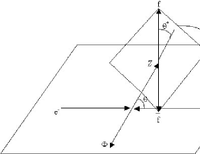
Figure 1: Definition of the production and decay angles of the process $e^{+}e^{-}\rightarrow Z\Phi[Z\rightarrow f\overline{f}$].

Figure 2: Angular distribution of the process $e^{+}e^{-}\rightarrow ZA$ obtained by the “re-weighting” method (See text) for an integrated luminosity of 500 $fb^{-1}$ and a center of mass energy of $\sqrt{s}=350$ GeV, assuming a Higgs mass of 120 GeV. The line indicates the exact theoretical dependence.

III Description of the method and Monte Carlo studies

We consider the production of Higgs events at the TESLA operating at a center-of-mass energy of 350 GeV, assuming an integrated luminosity of 500 $fb^{-1}$. At this energy the main production process for the Higgs boson in the SM is the Higgsstrahlung process, $e^{+}e^{-}\rightarrow ZH$ JE . The corresponding expected number of events for this process is $6.6\times 10^{4}$.

We have choosen for the present study the process $e^{+}e^{-}\rightarrow ZH\rightarrow\mu^{+}\mu^{-}H$ with a Higgs boson mass of 120 GeV. This decay channel exhibits a clean signature in the detector and the selection efficiencies are expected to be independent of the decay mode of the Higgs boson. We allow the produced Higgs to be either scalar or a mixture state $\Phi$ including an interference term.

All the Monte Carlo samples have been generated with the Pythia program as described in the previous section. These events are then passed through the simulation package SIMDET SD , a parametric Monte Carlo program for a TESLA detector SD2 which follows the proposal presented in the TESLA Conceptual Design Report DR . For the Higgs boson all decay modes are simulated as expected in the SM. The following background processes are considered in the analysis: $e^{+}e^{-}\rightarrow e^{+}e^{-}f^{+}f^{-}$, $e^{+}e^{-}\rightarrow f^{+}f^{-}(\gamma)$, $e^{+}e^{-}\rightarrow W^{+}W^{-}$ and $e^{+}e^{-}\rightarrow ZZ$. Both signal and background events are processed by the detector simulation package.

For the event selection we follow ref. MS2 . At least one muon and anti-muon are identified, with energy larger than 15 GeV. The mass of the di-muon system is required to be consistent with the Z boson hypothesis within 5 GeV. The recoil mass of the di-muon system $M^{2}_{rec}=(\sqrt{s}-(E_{\mu^{+}}+E_{\mu^{-}}))^{2}-(\vec{P}_{\mu^{+}}+\vec{P}_{\mu^{-}})^{2}$ has to be consistent with the H boson hypothesis within 5 GeV. This variable will yield a peak for the signal of the Higgs boson mass, independently of the Higgs boson decay mode. To remove a significant part of the remaining background, the absolute z-component of the di-muon system is required to be smaller than 120 GeV.

The momemtum of the selected muons are used to calculate the cosines of the production and decay angles for futher use in the method to determine the $J^{PC}$ properties of the Higgs boson. It has been noted in DR that having excellent momemtum and energy resolution will allow the Z to be well reconstructed. The recoil mass against the Z, can then be used to detect the Higgs boson and to study its properties. Figure 3 shows the recoil mass distribution for the $m_{H}=120$ GeV signal, obtained from the selected events in the sample of $e^{+}e^{-}\rightarrow ZH\rightarrow\mu^{+}\mu^{-}X$. The Higgs boson signal appears on top of a small background. In Figure  4 the corresponding $\cos\theta$ distribution is shown. The expected background is also presented. The combination of the cut on the z-component of the di-muon system, and the decreasing muon identification performance results in an efficiency for $\cos\theta>0.9$ close to zero.

Figure 3: Recoil mass spectra off the Z in $e^{+}e^{-}\rightarrow ZH\rightarrow\mu^{+}\mu^{-}X$. Shadowed area represents the expected background events.

Figure 4: Angular distribution, cos $\theta$, of the selected events in $e^{+}e^{-}\rightarrow ZH\rightarrow\mu^{+}\mu^{-}X$. The shaded histogram correspond to the expected background.

The kinematics of the $e^{+}e^{-}\rightarrow Z\Phi$ $[Z\rightarrow f\overline{f}]$ process is described by the production and decay angles $\theta$, $\theta^{*}$, $\phi^{*}$. The method we propose consists in generating 3-dimensional distributions in $\cos\theta$, $\cos\theta^{*}$ and $\cos\phi^{*}$ using the Monte Carlo events generated as described above for each contribution in equation (3). We write then the likelihood:

$${\cal L}=\prod_{(\cos\theta)_{i},(\cos\theta^{*})_{j},(\cos\phi^{*})_{k}}\frac{\mu_{ijk}{}^{N_{data}(i,j,k)}e^{-\mu_{ijk}}}{N_{data(i,j,k)}!}$$ (7)

where $N_{data}(i,j,k)$ is the number of events of the hypothetical data sample and $\mu_{ijk}$ is the expected number in the ijk-th bin. $\mu_{ijk}$ is calculated assuming a linear combination of the number of events of three Monte Carlo samples, corresponding to the production of scalar Higgs (MC_ZH), pseudoscalar (MC_ZA) Higgs and events for the interference term (MC_IN):

$$\mu_{ijk}={\cal N}.(\alpha.MC\_ZH_{ijk}+\beta.MC\_IN_{ijk}+\gamma.MC\_ZA_{ijk})$$ (8)

where $\cal N$ is the overall normalization factor between numbers of data and Monte Carlo events which can be fixed (${\cal N}=0.1$ in our case) or left free as a further check of the fit. The likelihood is then maximized with respect to $\alpha$, $\beta$ and $\gamma$. The absolute value of $\beta$ indicates the contribution of interference term in the sample and $\alpha$ and $\gamma$ indicate the fraction of scalar and pseudoscalar components respectively. A significant deviation of $\beta$ from zero would imply the existence of $\cal CP$ violation, independent of the specific model. For a scalar Higgs sample ($\eta=0$), the result of the fit is expected to be $\alpha=1$ and $\beta=\gamma=0$.

We have performed Monte Carlo studies with several hypothetical data samples with non-standard values of $\eta$. A maximum likelihood fit for the best linear combination of MC_ZH, MC_ZA and MC_IN to match the hypothetical data sample gave statistical errors of 0.04, 0.02 and 0.04 for $\alpha$, $\beta$ and $\gamma$, respectively. The results of these studies using different values of $\eta$ are given in table  1.

Table 1: Obtained values of the parameters for differents “data” samples

$\eta$	$\alpha$	$\beta$	$\gamma$
-0.4	0.002 $\pm$ 0.03	-0.05 $\pm$ 0.02	0.98 $\pm$ 0.04
-0.25	0.08 $\pm$ 0.04	-0.06 $\pm$ 0.02	0.92 $\pm$ 0.04
-0.1	0.43 $\pm$ 0.04	-0.09 $\pm$ 0.02	0.57 $\pm$ 0.04
-0.05	0.69 $\pm$ 0.04	-0.06 $\pm$ 0.02	0.31 $\pm$ 0.04
0	0.97 $\pm$ 0.05	0.003$\pm$ 0.02	0.03 $\pm$ 0.04
0.05	0.70 $\pm$ 0.05	0.05 $\pm$ 0.02	0.29 $\pm$ 0.04
0.1	0.40 $\pm$ 0.04	0.04 $\pm$ 0.02	0.59 $\pm$ 0.04
0.25	0.08 $\pm$ 0.04	0.04 $\pm$ 0.02	0.92 $\pm$ 0.04
0.4	0.002 $\pm$ 0.03	0.01 $\pm$ 0.02	0.98 $\pm$ 0.04

The value of $\alpha$ gives the fraction of the scalar $J^{PC}=0^{++}$ component of the Higgs boson, while $\gamma$ gives the contribution of the pseudoscalar Higgs component and increases quickly with $\eta$ as expected. It can be seen from our results that the Monte Carlo study using a sample of pure scalar SM-like Higgs gives a consistent answer. This indicates the high sensitivity of the method to distinguish a purely $\cal CP$-even state from a pseudoscalar $\cal CP$-odd state. Secondly, the method also allows one to determine whether the observed Higgs boson is a $\cal CP$ mixture and, if so, measure the odd and even component. It is evident that the statistical uncertainties prevent us to a large extent from measuring the interference term. It should be noted that for $Z\rightarrow\mu^{+}\mu^{-}$, as well as for $Z\rightarrow e^{+}e^{-}$, the interference term is suppressed by the smallness of $v_{f}$ independently of the size of $\eta$. However, the simultaneous existence of fractions $\alpha$ and $\gamma$ would indicate $\cal CP$ violation for the $ZZ\phi$ coupling. The method proposed here gives sensible results in the case that there is any significant $\cal CP$-even component in the $\phi$ Higgs boson or if $\phi$ is almost purely $\cal CP$-odd. The statististical significance can certainly be increased including the $e^{+}e^{-}\rightarrow e^{+}e^{-}X$ channel.

IV Summary

We have proposed a novel method for the measurement of the parity of the Higgs boson using the angular distributions of the differential cross section of $e^{+}e^{-}\rightarrow Z\phi$. The statistical power of our method using Monte Carlo generated hypothetical data samples is shown in Table  1. The results indicate that, for an integrated luminosity of $500fb^{-1}$, at 350 GeV centre-of-mass energy, TESLA will be able to unambiguosly determine whether a Higgs boson is a state $0^{++}$ ($\cal CP$-even, scalar) or has a contribution of the $0^{-+}$ ($\cal CP$-odd, pseudoscalar) state, like in general extensions of Higgs model. We also estimate the statistical uncertainties for the measurement of the $\cal CP$ violating interference term. We hope that this technique will allow confirmation of the expected $J^{PC}$ assignment of a Higgs boson candidate.

V Acknowledgments

We are greateful to W. Lohmann with whom early aspects of this idea were discussed. We would also like to thank L. Epele and P.Garcia-Abia for helpful discussions and T. Paul for carefully reading the manuscript. This work has been supported, in part by CONICET, Argentina. MTD thanks the John Simon Guggenheim Foundation for a fellowship.

References

- (1) F. Richard, J.R. Schnieder, D. Trines, A. Wagner. TESLA Technical Design Report (2001).
- (2) D0 Collaboration, V.M. Abazov et al. arXiv:hep-ex/0406031
- (3) E. Accomando, et al. ECFA/DESY LC, Phys. Rep.299 1 (1998).
- (4) V. Barger, K. Cheung, A Djoundi, B.A. Kniehl, P.M. Zerwas. Phys. Rev. D, 49 1 (1994).
- (5) B.A. Kniehl, Phys. Rep. 240, 211 (1994)
- (6) J.F. Gunion, H.E. Haber and R.V.Kooten, in “Higgs Physics at the LC” edited by K. Fujii, D.Miller and A.Soni (World Scientific) arXiv:hep-ph/0301023.
- (7) M.T.Dova, P. Garcia-Abia and W. Lohmann. LC-PHSM-2001-054 (http://www.desy.de/lcnotes/) and [arXiv:hep-ph/0302113]
- (8) P. W. Higgs, Phys. Rev. Lett. 12, 132 (1964).
- (9) J. Gunion, H. Haber, G. Kane and S. Dawson, The Higgs Hunter’s Guide (Addison-Wesley, Reading, 1990)
- (10) A. Djouadi, B. Kniehl. DESY 93-123 p. 51.
- (11) D.J. Miller, S.Y. Choi, B. Eberle, M.M.Muhlleitner, P.M. Zerwas. Phys. Lett. 505, 149 (2001).
-
(12)
K. Hagiwara and M.L.Stong, Z.Phys C62,99 (1994).
K.Hagiwara, S.Ishihara, J.Kamoshita and B.A. Kniehl, Eur. Phys. J.C14, 457 (2000). - (13) T.Han and J.Jiang, Phys. Rev. D63, 096007 (2001).
- (14) B.A. Kniehl. Int.J.Mod.Phys. A17 (2002) 1457-1476. [arViv:hep-ph/0112023].
- (15) M. Schumacher, LC-PHSM-2001-003.
- (16) V.D. Derwent et al.,Linear Collider Physics FERMILAB-FN-701 [arXiv:hep-ex/0107044]
- (17) K. Desch, A. Imhof, Z. Was and M.Worek, Phys. Lett. B579 157 (2004).
- (18) T. Sjöstrand, Comp. Phys. Comm. 135, 238 (2001).
- (19) J. Ellis, M.K. Gaillard, D.V. Nanopoulos. Nucl. Phys. B106, 292 (1976); B.L. Ioffe, V.A. Khoze. Sov. J. Nucl. Phys. 9, 50 (1978); B.W. Lee, C. Quigg, H.B. Thacker. Phys. Rev. 16,1519 (1977).
- (20) M.Pohl and H.J.Schreiber, report DESY 02-061, [arXiv:hep-ex/0206009] and LC-DET-2002-005.
- (21) T. Behnke, S. Bertolucci, R.D. Heuer and R. Sttels, TESLA Technical Design Report Part IV: A detector for TESLA, DESY-01-011