LRG Production of Di-Jets As a

Probe of s-Channel Unitarity

Uri MAOR ${\!}^{\mbox{\scriptsize 1)}}$

School of Physics and Astronomy
Raymond and Beverly Sackler Faculty of Exact Science
Tel Aviv University, Tel Aviv, 69978, ISRAEL

THIS PAPER IS DEDICATED TO PROF. ROBERTO SALMERON
ON HIS 80th BIRTHDAY

Abstract: Hard diffractive production of di-jets in the Tevatron and HERA are explored. It is argued that a consistent pQCD description of these data can be attained after s-channel unitarity re-scattering screening corrections are incorporated in the calculation. To this end a simple procedure is presented in which information derived from the measured soft total, elastic and diffractive cross sections simplifies the calculation and makes it parameter free. The above approach eliminates the inconsistencies seemingly observed when comparing the rates of diffractive di-jets production in different channels.

1 Introduction

A large rapidity gap (LRG) in an hadronic or DIS final state is experimentally defined as a large gap in the $\eta-\phi$ lego plot where no hadrons are produced. A schematic description of a LRG di-jet diffractive final state is shown in Fig. 1. Historically, LRG events where singled out[1][2] as a signature for Higgs production due to a $W-W$ fusion sub process in hadron-hadron collisions at exceedingly high energies. At presently available energies, LRG di-jet central production is observed in the Tevatron[3][4][5] and HERA[6]. These measurements provide a unique opportunity to assess the asymptotic short distance behavior of the hard diffractive sub process responsible for the LRG di-jet in the final state and check our ability to adequately calculate it utilizing perturbative QCD (pQCD) methods.

Figure 1: Lego plot for double diffractive dissociation.

The production of two hard jets separated by a LRG can be explained by either:
1) A fluctuation in the rapidity distribution of an inelastic event. The probability for such a fluctuation is proportional to $e^{-\Delta y/L}$, where $\Delta y=y_{1}-y_{2}$ and $L$ denotes the value of the correlation length. In a LRG event $\Delta y\gg L$ and, thus, the probability for such a fluctuation is very small. Or:
2) A QCD colorless t-channel exchange. We denote this exchange as a ”hard Pomeron”. Accordingly, we shall be interested in $F_{s}$, the ratio between the LRG and the inclusive cross sections for di-jet production. It was noted by Bjorken[2] that we have to distinguish between the calculated pQCD ratio $F_{s}$ and the actual measured ratio $f_{gap}$, where the proportionality factor is called the ”survival probability of a LRG”,

$$f_{gap}\,=\,\langle{\mid S\mid}^{2}\rangle\cdot F_{s}\,.$$ (1)

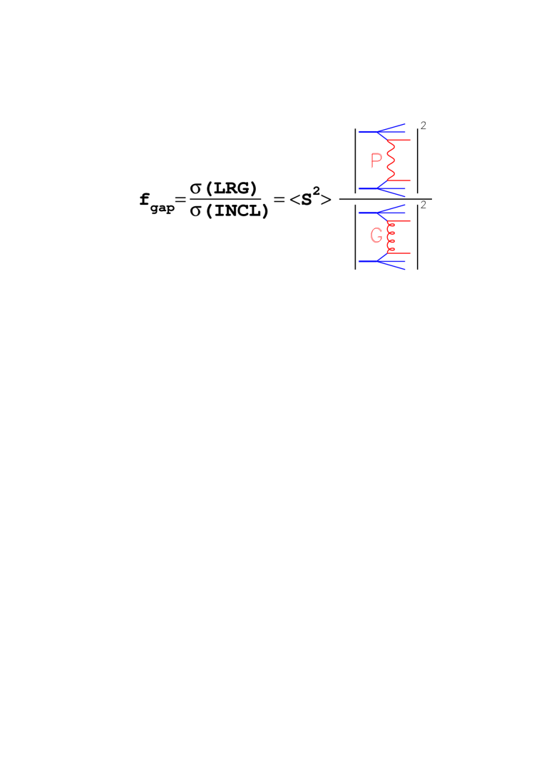
Figure 2: Pictorial definition of $f_{gap}$. P and G represent color singlet and octet respectively.

There have been several suggestions how to calculate the survival probability.
1) A simple procedure[7] has been suggested by Gotsman, Levin and Maor (GLM) to calculate $\langle{\mid S\mid}^{2}\rangle$. The procedure is based on the GLM model[8] which incorporates the effects of s-channel unitarity in high energy soft scattering. In the following I shall present this approach in some detail.
2) An alternative procedure has been suggested by the Durham group[9]. It will be discussed briefly in Sec. 6.
3) Another alternative proposal[10], associates the LRG phenomena with the color evaporation model (CEM). Like the previous listed options it explains the observed low values of the survival probability using the interplay between hard and soft physics. I shall discuss it very briefly in Sec. 6.

The survival probability is the probability of a given LRG not to be filled by debris (partons and/or hadrons). These debris can originate from the soft rescattering of the spectator partons, and/or from the gluon radiation emitted by partons taking part in the hard interaction

$$\langle{\mid S(s,\Delta y)\mid}^{2}\rangle\,=\,\langle{\mid S_{brem}(\Delta y)\mid}^{2}\rangle\cdot\langle{\mid S_{spec}(s)\mid}^{2}\rangle.$$ (2)

$\langle{\mid S_{brem}\mid}^{2}\rangle$ can be calculated in pQCD[11]. Its estimate[9], at presently available energies, is considerably smaller than $\langle\,{\mid S_{spec}\mid}^{2}\rangle$.

The need for a reliable calculation of the survival probability is evident once we note that the values of $f_{gap}$, measured at the Tevatron[3][4] and HERA[6], are very small and energy dependent:

$$f_{gap}(\sqrt{s}=\,\,630\,GeV)\,=\,1.60\pm 0.20\%\,(D0),\,and\,\,2.70\pm 0.90\%\,\,(CDF),$$ (3)

$$f_{gap}(\sqrt{s}=1800\,GeV)\,=\,0.60\pm 0.20\%\,(D0),\,and\,\,1.13\pm 0.16\%\,\,(CDF),$$ (4)

$$f_{gap}(\sqrt{s}=\,\,150\,GeV)\,=\,7.00\pm 2.00\%\,\,(ZEUS).$$ (5)

These numbers are considerably smaller, and reduce with increasing energy, in contradiction to the pQCD expectations. These observations can be understood only if $\langle{\mid S\mid}^{2}\rangle$ is rather small and energy dependent. Indeed, a direct measurement of the energy dependence of $f_{gap}$ by D0[3] gives

$$\frac{f_{gap}(\sqrt{s}=\,\,630\,GeV)}{f_{gap}(\sqrt{s}=1800\,GeV)}\,=\,3.4\pm 1.3,$$ (6)

to be compared with a ratio of $2.7\pm 0.6$ obtained from the individual numbers just quoted (Eq. (3) and Eq. (4)). As stated, the purpose of this short review is to present a relatively simple, and parameter free, procedure to calculate the survival probability and correlate its small value with the properties of high energy soft scattering. I shall show that the Tevatron data is perfectly consistent with the HERA data and that the calculations yield a natural interpretation of LRG di-jets observed in different channels. An important consequence of this analysis is that it provides significant support for the need to implement s-channel unitarity corrections to soft hadronic interactions in the HERA - Tevatron energy range.

The organization of this paper is as follows: In Sec. 2 I briefly review the roll of s-channel unitarity in high energy soft scattering and its implications. This is followed in Sec. 3 by a suggested model by GLM[8], compatible with unitarity constraints, which is based on the eikonal approximation. The calculation of the survival probabilities in the eikonal approach are presented and discussed in Sec. 4. The procedure presented incorporates the soft scattering basic measurements which replaces the need for free parameters. A generalization to a multi channel rescattering model is briefly reviewed in Sec. 5. A short discussion is presented in Sec. 6.

2 s-Channel Unitarity in High Energy Soft Scattering

High energy soft scattering is commonly described by the Regge-pole model[12]. The theory was introduced more than 40 years ago and was soon after followed by a very rich phenomenology. The two key ingredients of this approach are the Pomeron whose t dependent trajectory is given by

$$\alpha_{P}(t)\,=\,\alpha_{P}(0)\,+\,\alpha_{P}^{\prime}t,$$ (7)

and a leading Regge trajectory

$$\alpha_{R}(t)\,=\,\alpha_{R}(0)\,+\,\alpha_{R}^{\prime}t.$$ (8)

Donnachie and Landshoff (DL) have vigorously promoted[13] an appealing and very simple Regge parametrization for total and forward differential elastic hadron-hadron cross sections in which

$$\sigma_{tot}\,=\,X\left(\frac{s}{s_{0}}\right)^{\epsilon}\,+\,Y\left(\frac{s}{s_{0}}\right)^{-\eta},$$ (9)

and

$$\frac{d\sigma_{el}}{dt}\,=\,\left(\frac{d\sigma_{el}}{dt}\right)_{0}e^{B_{el}t}.$$ (10)

$\left(\frac{d\sigma_{el}}{dt}\right)_{0}$ and $\sigma_{tot}$ are related through the optical theorem. The forward elastic high energy exponential slope is given by

$$B_{el}\,=\,B_{0}\,+\,2\alpha_{P}^{\prime}ln\left(\frac{s}{s_{0}}\right).$$ (11)

The data is excellently fitted with universal parameters:
1) A supercritical Pomeron with an intercept $\alpha_{P}(0)\,=\,1\,+\,\epsilon$, where $\epsilon\,=\,0.08$ accounts for the high energy growing total cross sections. Its fitted[14] slope value is $\alpha_{P}^{\prime}\,=\,0.25\,GeV^{-2}$.
2) The low energy data is controlled by the leading Regge trajectory whose universal parameters are[13] $\eta\,=\,0.45$ and $\alpha_{R}^{\prime}\,=\,1\,GeV^{-2}$.
DL offer a global fit to all available hadron-hadron and photon-hadron total and elastic cross section data. Note, though, that in reality only $\bar{p}p$ and $\gamma p$ reactions have attained high enough energies in which the Pomeron parameters can be tested. We also note that the comprehensive DL analysis is limited to the properties of the elastic amplitude with no reference to diffractive scattering.

Elastic and diffraction dissociation are similar processes which have predominantly forward imaginary amplitudes corresponding to the exchange of vacuum quantum numbers in the t-channel. As such, both channels are dominated in the high energy limit by a Pomeron exchange and are expected, in a simple Regge model, to exhibit rather similar dependences on the kinematic variable. Indeed, in the triple Regge limit applied to high energy single diffraction (SD) we get[15]

$$\frac{M^{2}d\sigma_{sd}}{dM^{2}dt}\,=\,\sigma^{2}(s_{0})\left(\frac{s}{M^{2}}\right)^{2\epsilon+2\alpha_{P}^{\prime}t}G_{PPP}\left(\frac{M^{2}}{s}\right)^{\epsilon},$$ (12)

where $M$ is the diffracted mass, and $G_{PPP}$ is the triple Pomeron vertex coupling. The virtue of this formalism is that it provides a strong correlation between the energy dependences of $\sigma_{tot},\sigma_{el},B_{el}$, and the energy and $M^{2}$ dependences of $\sigma_{sd}$.

The simple model just presented is bound, eventually, to violate s-channel unitarity since $\sigma_{el}$ and $\sigma_{sd}$ grow with energy as $s^{2\epsilon}$, modulu logarithmic corrections, while $\sigma_{tot}$ grows only as $s^{\epsilon}$. The detailed theoretical problems at stake are easily identified in an impact b-space formalism which is outlined below.

The elastic scattering amplitude is normalized so that

$$\frac{d\sigma_{el}}{dt}\,=\,\pi\mid f_{el}(s,t)\mid^{2},$$ (13)

and

$$\sigma_{tot}\,=\,4\pi Imf_{el}(s,0).$$ (14)

The elastic amplitude in b-space is defined as

$$a_{el}(s,b)\,=\,\frac{1}{2\pi}\int d{\bf q}e^{-i{\bf q\cdot b}}f_{el}(s,t),$$ (15)

where $t\,=\,-q^{2}$. In this representation

$$\sigma_{tot}\,=\,2\int d{\bf b}Ima_{el}(s,b),$$ (16)

$$\sigma_{el}\,=\,\int d{\bf b}\mid a_{el}(s,b)\mid^{2}.$$ (17)

The common formulation of s-channel unitarity implies that $\mid a_{el}(s,b)\mid\leq 1$, which is the black bound. We also have the analyticity/crossing bound. The position of this bound depends on the mass of the lightest exchange in the t-channel. Froissart[16], at the time, considered it to be a $\pi$ meson. Our present thinking tends to consider it as the lightest glue-ball which can be exchanged in the $t$ channel. The Froissart bound is obtained when the unitarity and analyticity/crossing bounds are combined.

$$\sigma_{tot}\,\leq\,C\,ln\left(\frac{s}{s_{0}}\right),$$ (18)

where $C$ depends on the crossed channel exchanged mass. Note that both the unitarity and Froissart bounds are numerical, not functional. Consequently, the Froissart bound (with any reasonable value of $C$) is not applicable to present day accelerator physics, being much higher than the actual data.

Figure 3: A pictorial illustration of a high energy b-space elastic amplitude bounded by unitarity and analyticity/crossing. In the illustration we have an input amplitude which violates the unitarity bound and an output amplitude obtained after a unitarization procedure.

On the other hand, as we shall see, the unitarity bound is very relevant to the analysis of the presently available high energy data. A schematic illustration of the above is presented in Fig. 3.

As noted, a simple Regge pole parametrization will eventually violate s-channel unitarity since the integrated elastic and diffractive cross sections grow with s much faster than the total cross section. The question is if this is a future problem to be confronted only at far higher energies than presently available, or is it a phenomena which can be identified through experimental signatures observed within the available high energy data base. It is an easy exercise to check that the DL model[13], with its fitted global parameters, will violate the unitarity black limit for small b just above the present Tevatron energy. Indeed, CDF reports[17] that $a_{el}(b=0,\sqrt{s}=1800)\,=\,0.96\pm 0.04$. In a DL type model this should be reflected in $\epsilon$ acquiring an energy dependence rather than the fixed fitted value. This is not observed, as yet, in the total and elastic cross section available data. We note, though, that the energy dependence of the experimental SD cross section[5] in the ISR-Tevatron energy range is much weaker than the power dependences observed for $\sigma_{el}$. This observation is dramatically demonstrated once we check the ratio between $\left(\frac{d\sigma_{sd}}{dt}\right)_{0}$ and $\left(\frac{d\sigma_{el}}{dt}\right)_{0}$ which goes down with energy.

3 The GLM Screening Correction Model

The theoretical difficulties, pointed out in the previous section, are eliminated once we take into account the corrections necessitated by unitarity. The problem is that enforcing unitarity is a model dependent procedure. In the following I shall confine myself to the GLM screening corrections (SC) model[8]. In this semi realistic model the unitarity enforced SC are calculated utilizing a Glauber type eikonal approximation in which the scattering matrix is diagonal and only repeated elastic rescatterings are summed. Accordingly, we write

$$a_{el}(s,b)\,=\,i\left(1-e^{-\Omega(s,b)/2}\right),$$ (19)

where the opacity $\Omega$ is a real function which is identified with the value of the imaginary part of a DL input super critical Pomeron. Analyticity and crossing symmetry are easily restored by the substitution $s^{\alpha_{P}}\,\rightarrow\,s^{\alpha_{P}}e^{-i\pi\alpha_{P}/2}$. Combining Eq. (16), Eq. (17) and Eq. (19) we get

$$\sigma_{tot}\,=\,2\int d^{2}b\left(1\,-\,e^{-\Omega(s,b)/2}\right),$$ (20)

and

$$\sigma_{in}\,=\,2\int d^{2}b\left(1\,-\,e^{-\Omega(s,b)}\right).$$ (21)

Since the scattering matrix is diagonal, the unitarity constraint is written as

$$2Ima_{el}(s,b)\,=\,{\mid a_{el}(s,b)\mid}^{2}\,+\,G^{in}(s,b).$$ (22)

Note that Eq. (19) is a solution of Eq. (22). We also get

$$G^{in}\,=\,1\,-\,e^{-\Omega(s,b)}.$$ (23)

The eikonal approximation can be summed analytically with a Gaussian input which corresponds to an exponential representation of the scattering amplitude in t-space (see Eq. (10)). This is, clearly, an over simplification, but it reproduces well the small t elastic cross section which contains the bulk of the data.

$$\Omega(s,b)\,=\,\sigma(s_{0})\Gamma_{S}(s,b)\,=\,\nu(s)e^{\frac{-b^{2}}{R_{S}^{2}(s)}},$$ (24)

where

$$\nu(s)\,=\,\Omega(s,b=0)\,=\,\frac{\sigma(s_{0})}{\pi R_{S}^{2}(s)}\left(\frac{s}{s_{0}}\right)^{\Delta},$$ (25)

and

$$R_{S}^{2}(s)\,=\,4R_{0}^{2}\,+\,4\alpha_{P}^{\prime}ln(\frac{s}{s_{0}}).$$ (26)

The soft profile is defined

$$\Gamma_{S}(s,b)\,=\,\frac{1}{\pi R_{S}^{2}(s)}e^{-\frac{b^{2}}{R_{S}^{2}(s)}}.$$ (27)

Some clarifications are in order so as to distinguish between the GLM model input and output:
1) The power $\Delta$, and accordingly $\nu$, are input information and should not be confused with DL effective power $\epsilon$ and its corresponding cross section. Obviously, $\Delta\,>\,\epsilon$.
2) The relation $B_{el}\,=\,\frac{1}{2}R_{S}^{2}(s)$ depends mostly on the high $b$ tail of the profile $\Gamma_{S}$. As such, SC do not change the output soft radius and this relation significantly.

With this input we get

$$\sigma_{tot}\,=\,2\pi R_{S}^{2}(s)\left(ln(\frac{\nu(s)}{2})\,+\,C\,-\,Ei(-\frac{\nu(s)}{2})\right)\,\propto\,ln^{2}(s),$$ (28)

$$\sigma_{in}\,=\,\pi R_{S}^{2}(s)\left(ln[\nu(s)]\,+\,C\,-\,Ei[-\nu(s)]\right)\,\propto\,\frac{1}{2}ln^{2}(s),$$ (29)

$$\sigma_{el}\,=\,\sigma_{tot}\,-\,\sigma_{in}\,=\,\pi R_{S}^{2}(s)\left(ln(\frac{\nu(s)}{4})\,+\,C\,-\,2Ei(-\frac{\nu(s)}{2})\,+\,Ei[-\nu(s)]\right)\,\propto\,\frac{1}{2}ln^{2}(s),$$ (30)

where $Ei(x)\,=\,\int_{-\infty}^{x}\frac{e^{t}}{t}dt$, and $C\,=\,0.5773$ is the Euler constant.

The formalism just presented can be extended[8] also to diffractive channels. The key observation is traced to Eq. (23) from where we define

$$P_{S}(s,b)\,=\,e^{-\Omega(s,b)}$$ (31)

to be the probability that the two initial hadrons do not interact inelastically. i.e. there is no initial state rescattering in the inelastic sector at the given $s,b$ values. Accordingly, the screened diffractive cross section is obtained by multiplying its b-space amplitude by this probability. In this approximation rescatterings in the diffractive final state are not included. Specifically, for SD we take the b-space transform of Eq. (12) multiplied by $P_{S}(s,b)$ and obtain after integration

$$\frac{M^{2}d\sigma_{sd}}{dM^{2}}\,=\,\frac{\sigma^{2}(s_{0})}{2\pi\bar{R}_{S}^{2}(\frac{s}{M^{2}})}\left(\frac{s}{M^{2}}\right)^{2\Delta}G_{PPP}\left(\frac{M^{2}}{s_{0}}\right)^{\Delta}a_{D}(s,M^{2})\frac{1}{[2\nu(s)]^{a_{D}(s,M^{2})}}\gamma[a_{D}(s,M^{2}),2\nu(s)],$$ (32)

where

$$\bar{R}_{S}^{2}\left(\frac{s}{M^{2}}\right)\,=\,2R_{0}^{2}\,+\,r_{0}^{2}\,+\,4\alpha_{P}^{\prime}ln\left(\frac{s}{M^{2}}\right).$$ (33)

$r_{0}\leq 1GeV^{-2}$ denotes the radius of the triple Pomeron vertex and can be safely neglected. Note that $\frac{1}{2}R_{S}^{2}\,<\,{\bar{R}}_{S}^{2}\,<\,R_{S}^{2}$. In the ISR-Tevatron energy range ${\bar{R}}_{S}^{2}$ is just moderately larger than $\frac{1}{2}R_{S}^{2}$.

$$a_{D}(s,M^{2})\,=\,\frac{2R_{S}^{2}(s)}{\bar{R}_{S}^{2}(\frac{s}{M^{2}})\,+\,2\bar{R}_{S}^{2}(\frac{M^{2}}{s_{0}})}.$$ (34)

$\gamma(a,2\nu)$ denotes the incomplete Euler gamma function

$$\gamma(a,x)\,=\,\int_{0}^{x}\,z^{a-1}e^{-z}dz.$$ (35)

In the high energy limit Eq. (32) simplifies to

$$\frac{M^{2}d\sigma_{sd}}{dM^{2}}\,=\,\pi R_{S}^{2}(s)G_{PPP}\left(\frac{M^{2}}{s_{0}}\right)^{\Delta}\,\propto ln(s).$$ (36)

The simple model, just presented, provides a significant improvement on the Regge DL model which serves as its input:
1) It is compatible with unitarity (and Froissart) behavior in the high energy limit. In particular, the asymptotic ratio of $\frac{\sigma_{el}}{\sigma_{tot}}$ is kept at $\frac{1}{2}$ (Eq. (28) - Eq. (30)).
2) Even though both $\sigma_{tot}$ and $\sigma_{el}$ change, at high enough energies, their dependence on $s$ from a power to a $ln^{2}(s)$ behavior, this change will be experimentally observed at an energy far higher than presently available. The model is, thus, compatible with DL in the ISR-Tevatron energy range.
3) The SD cross section changes its power dependence on $s$ to a $ln(s)$ behavior. Checking the numerics of Eq. (36) this change is significant in the ISR-Tevatron energy range. Note that in the high energy limit $\frac{\sigma_{diff}}{\sigma_{tot}}$ vanishes like $\frac{1}{ln(s)}$.
4) The significant difference between the energy dependence of the seemingly similar elastic and SD (and other diffractive) cross sections is understood once we examine their b-space amplitudes. The elastic amplitude is central (approximately given by a central Gaussian). Its DL parametrization implies that $a_{el}(s,b)$ will violate unitarity at small b somewhere between 2 and 3 $TeV$ c.m. energy. Since this is confined to exceedingly small b values, it translates to very small changes in the normalization of the total and elastic cross sections. Screening is very different for the SD b-space amplitude. The screening suppression is obtained from the multiplication by $P_{S}(s,b)$, of Eq. (31), which is very small at small b and approaches unity at higher b values. Whereas the screened elastic b-space amplitude maintains its centrality with a maximum at $b\,=\,0$, the screened SD amplitude changes from a central to a peripheral b distribution, which is accompanied by a significant reduction of the output SD cross section. This phenomena is compatible with the Pumplin bound[18] in which the sum of the elastic and diffractive b-space amplitudes is bounded by $\frac{1}{2}$.

Regardless of its qualitative success, the toy GLM model does not provide a realistic reproduction of the data. Its two important deficiencies are:
1) The model does not produce a good reproduction of the SD data[5]. This is amended in a multi channel eikonal model[7] in which diffractive intermediate rescatterings are also included.
2) The model is applicable only for small $t$ elastic scattering and it does not reproduce the high $t$ diffractive dip experimentally observed at high energies. This is a consequence of our usage of a Gaussian b profile. To improve this deficiency we have to use a more elaborate profile[19].

4 Survival Probability of LRG in the GLM Model

Following Bjorken[2], the survival probability, associated with the soft rescatterings of the spectator partons, is defined as the normalized integrated product of two quantities:

$$\langle{\mid S_{spec}\mid}^{2}\rangle\,=\,\frac{\int d^{2}b\Gamma_{H}(s,b)P_{S}(s,b)}{\int d^{2}b\Gamma_{H}(s,b)}.$$ (37)

1) The first element in Eq. (37) is a convolution over the parton densities of the two interacting hadronic projectiles. This provides the uncorrected hard parton-parton collision cross section, leading, in our context, to di-jets. Following the discussion of soft scattering in Sec. 2, we assume a Gaussian hard profile

$$\Gamma_{H}\,=\,\frac{1}{\pi R_{H}^{2}(s)}e^{-\frac{b^{2}}{R_{H}^{2}(s)}},$$ (38)

where $R_{H}$ denotes the radius of the hard scattering process. This choice enables an analytical solution of Eq. (37). More elaborate choices require a numerical evaluation of this equation.
2) The second element is the probability $P_{S}(s,b)$, defined in Eq. (31), that no inelastic soft interaction takes place between the incoming projectiles at impact parameter $b$ and c.m. energy square $s$. We define

$$a_{H}(s)\,=\,\frac{R_{S}^{2}(s)}{R_{H}^{2}(s)}\,=\,\frac{interaction\,area\,for\,soft\,collisions}{interaction\,area\,for\,hard\,collisions}\,>\,1.$$ (39)

$a_{H}(s)$ grows logarithmically with $s$. As stated, Eq. (37) can be analytically evaluated with our choice of Gaussian profiles and we get

$$\langle{\mid S_{spec}\mid}^{2}\rangle\,=\,\frac{a_{H}(s)\gamma[a_{H}(s),\nu(s)]}{[\nu(s)]^{a_{H}(s)}}.$$ (40)

$\nu(s)$ was defined in Eq. (25) and the $\gamma$ function in Eq. (35).

A straight forward estimate of the LRG survival probabilities can be derived[2][7][9][10] from various models assumed to describe the soft and hard interactions. An alternative method suggested by GLM[7] is based on the GLM eikonal model reviewed in Sec. 3. This calculation of $\langle{\mid S_{spec}\mid}^{2}\rangle$ is executed with no further recourse to the theoretical models, utilizing just the experimental data from which we can directly deduce the input needed to solve Eq. (40). To this end we have to assess the values of $R_{H}^{2}$, $R_{S}^{2}$ and $\nu(s)$.

The value of $R_{H}^{2}$ is estimated from two independent experiments:
1) In analogy to the relation $R_{S}^{2}\,\simeq 2B_{el}$, we can estimate the value of the hard radius from the exponential slope of a clean hard process $R_{H}^{2}\,\simeq 2B_{hard}$. We use the excellent HERA data[20] on $\gamma+p\rightarrow J/\Psi+p$, where $B_{J/\Psi}\,\simeq\,4GeV^{-2}$ with a small logarithmic dependence on the incoming energy.
2) The above is compatible with the CDF estimate of the double parton cross section. This cross section is connected through factorization to the effective hard cross section

$$\sigma_{DP}\,=\,m\frac{\sigma_{incl1}(2\,jets)\,\sigma_{incl2}(2\,jets)}{2\sigma_{eff}^{H}},$$ (41)

where the factor $m$ is equal to 1 for identical pairs and 2 for different pairs. $\sigma_{eff}^{H}$ relates directly to the hard profile (Eq. (38))

$$\frac{1}{\sigma_{eff}^{H}}\,=\,\frac{1}{2\pi R_{H}^{2}}\,=\,\int d^{2}b\Gamma_{H}^{2}(b).$$ (42)

The experimental value[21] $\sigma_{eff}^{H}\,=\,14.5\pm 1.7\pm 2.3\,mb$ suggests that $R_{H}^{2}\,=\,5-7GeV^{-2}$.
In our calculations we took the HERA deduced value $R_{H}^{2}\,=\,8GeV^{-2}$. This is a conservative choice which may be slightly changed with the improvement of the Tevatron estimates.

The values of $R_{S}^{2}(s)$ are taken from the experimental elastic slope of the high energy $\bar{p}p$ data. The values of $\nu(s)$ can be obtained in the GLM model directly from the measured values of $\frac{\sigma_{el}}{\sigma_{tot}}$. Checking Eq. (28) and Eq. (30). We note that the (s dependent) ratio of elastic to total high energy cross sections provides explicit information on $\nu(s)$. Once we have determined $\nu(s)$ and $a_{H}(s)$, the survival probability is obtained from Eq. (40).

The important result of our calculation, which is displayed in Fig. 4, is that $\langle{\mid S_{spec}\mid}^{2}\rangle$

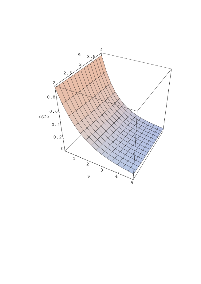
Figure 4: $\langle{\mid S_{spec}\mid}^{2}\rangle$ as a function of $\nu(s)$ and $a_{H}(s)$.

decreases as we go to higher energies. This is traced to the experimentally observed increase with energy of $\nu(s)$ and $a_{H}(s)$. To further illustrate this feature, we show a contour plot of

Figure 5: A contour plot of $\langle{\mid S_{spec}\mid}^{2}\rangle$ against $\nu(s)$ and $a_{H}(s)$.

$\langle{\mid S_{spec}\mid}^{2}\rangle$ against $\nu(s)$ and $a_{H}(s)$ in Fig. 5.

Our results for the survival probability at the reported energies:

$\sqrt{s}\,\,$(GeV)	$\langle{\mid S_{spec}\mid}^{2}\rangle$
150	16.3%
630	12.8%
1800	5.9%

provide a qualitative explanation for the smallness and energy dependence observed experimentally. However, for a quantitative comparison between the reported $f_{gap}$ data (Eq. (3) - Eq. (5)) and our results we have to incorporate a pQCD estimate of $F_{s}$. I shall return to this issue in the discussion. To bypass this difficulty it is constructive to check the ratio of the survival probabilities calculated at 630 and 1800 $GeV$

$$\frac{{\langle{\mid S_{spec}\mid}^{2}\rangle}_{\sqrt{s}\,=\,630}}{{\langle{\mid S_{spec}\mid}^{2}\rangle}_{\sqrt{s}\,=\,1800}}\,=\,2.2\pm 0.2.$$ (43)

Our calculated ratio is fully substantiated by the D0 result[3] in which the corresponding survival probability (rather than the $f_{gap}$) ratio was estimated at $2.2\pm 0.8$. Note that for our calculations at 630 $GeV$ we had to interpolate the input data information from 546 $GeV$.

5 Extension to a Multi Channel Model

In as much as the GLM results on the survival probability are very satisfactory, the over all quality of the GLM predictions is not that good. The GLM model[8] was originally conceived so as to explain the exceptional mild energy dependence of soft diffractive cross sections. It suggested that a high energy change from a power to a logarithmic energy dependence of the diffractive cross sections is a signature indicating the onsetting of s-channel unitarity corrections. The model actual calculations do, indeed, result in a qualitative significant difference between the energy dependence of the total and elastic cross sections, on the one hand, and diffractive cross sections, on the other hand. However, they do not provide an adequate reproduction of the SD cross sections[5] in the ISR-Tevatron energy range. A possible remedy to this deficiency of the GLM model is to replace the one channel eikonal model, in which only elastic rescatterings are included, with a multi channel eikonal model in which inelastic diffractive intermediate rescatterings are included as well. This is not a difficult technical problem[22], but, in our context, we have to secure that a multi channel model does improve the diffractive (specifically SD) predictions of the GLM model, while maintaining, simultaneously, its excellent results on LRG[7].

The implicit assumptions of the simple GLM model are:
1) Hadrons are the correct degrees of freedom at high energies.
2) At high energy $Re\,a_{el}\,\ll\,Im\,a_{el}$.
3) $\sigma_{diff}\,\ll\,\sigma_{el}$.
4) Only the fastest partons can interact with each other.
Clearly, the last two assumptions are the weakest of the four. There is no question that at small enough $x$ (high enough energy) one has to take into account $\langle{\mid S_{brem}(s)\mid}^{2}\rangle$. However, an explicit pQCD calculation[11] has shown it to be rather small in the energy range of interest, i.e. ISR-Tevatron. Here, I present a re-formulation of the GLM model. The goal is to construct a multi channel eikonal model in which the rescattering can be either elastic or diffractive.

In the simplest approximation we consider diffraction as a single hadronic state. We have, thus, two orthogonal wave functions

$$\langle\Psi_{h}\mid\Psi_{d}\rangle\,=\,0.$$ (44)

$\Psi_{h}$ is the wave function of the incoming hadron, and $\Psi_{D}$ is the wave function of the outgoing diffractively produced particles, initiated by the incoming hadron. Denote the interaction operator by T and consider two wave functions $\Psi_{1}$ and $\Psi_{2}$ which are diagonal with respect to T. The amplitude of the interaction is given by

$$A_{i,k}\,=\,\langle\Psi_{i}\Psi_{k}\mid{\bf T}\mid\Psi_{i^{\prime}}\Psi_{k^{\prime}}\rangle\,=\,A_{i,k}^{el}\,\,\delta_{i,i^{\prime}}\,\,\delta_{k,k^{\prime}}.$$ (45)

In a $2\times 2$ model $i,k\,=\,1,2$. The amplitude $A_{i,k}^{el}$ satisfies the diagonal unitarity condition (see Eq. (22))

$$2Im\,A_{i,k}^{el}(s,b)\,=\,\mid A_{i,k}^{el}(s,b)\mid^{2}\,+\,G_{i,k}^{in}(s,b),$$ (46)

for which we write the solution

$$A_{i,k}^{el}(s,b)\,=\,i\left(1\,-\,e^{-\frac{\Omega_{i,k}(s,b)}{2}}\right),$$ (47)

and

$$G_{i,k}^{in}\,=\,1-e^{-\Omega_{i,k}(s,b)}.$$ (48)

$\Omega_{i,k}(s,b)$ is the opacity of the $(i,k)-th$ channel with a wave function $\Psi_{i}\,\times\,\Psi_{k}$. The probability that two hadronic states $i$ and $k$ do not interact inelastically is

$$P_{i,k}(s,b)\,=\,e^{-\Omega_{i,k}(s,b)}\,=\,\{1\,-\,A_{i,k}^{el}(s,b)\}^{2}.$$ (49)

In this representation $\Psi_{h}$ and $\Psi_{d}$ can be written as

$$\Psi_{h}\,=\,\alpha\Psi_{1}\,+\,\beta\Psi_{2},$$ (50)

$$\Psi_{d}\,=\,-\beta\Psi_{1}\,+\,\alpha\Psi_{2}.$$ (51)

Since $\mid\Psi_{h}\mid^{2}\,=\,1$, we have

$$\alpha^{2}\,+\,\beta^{2}\,=\,1.$$ (52)

The wave function of the final state is

$$\Psi_{f}\,=\,\mid{\bf T}\mid\Psi_{h}\times\Psi_{h}\rangle\,=\,\alpha^{2}A_{1,1}\Psi_{1}\times\Psi_{1}\,+\,\alpha\beta A_{1,2}\{\Psi_{1}\times\Psi_{2}\,+\,\Psi_{2}\times\Psi_{1}\}\,+\,\beta^{2}A_{2,2}\Psi_{2}\times\Psi_{2}.$$ (53)

Since $A_{i,k}^{el}$ is a $2\times 2$ matrix, we have to consider 4 possible rescattering processes. However, in the case of a $\bar{p}p$ (or $pp$) collision, single diffraction at the proton vertex equals single diffraction at the antiproton vertex. i.e. $A_{1,2}\,=\,A_{2,1}$ and we end with 3 channels whose b-space amplitudes are given by

$$a_{el}(s,b)\,=\,\langle\Psi_{h}\times\Psi_{h}\mid\Psi_{f}\rangle\,=\,\alpha^{4}A_{1,1}\,+\,2\alpha^{2}\beta^{2}A_{1,2}\,+\,\beta^{4}A_{2,2},$$ (54)

$$a_{sd}(s,b)\,=\,\langle\Psi_{h}\times\Psi_{d}\mid\Psi_{f}\rangle\,=\,\alpha\beta\{\-\alpha^{2}A_{1,1}\,+\,(\alpha^{2}\,-\,\beta^{2})A_{1,2}\,+\,\beta^{2}A_{2,2}\},$$ (55)

$$a_{dd}(s,b)\,=\,\langle\Psi_{d}\times\Psi_{d}\mid\Psi_{f}\rangle\,=\,\alpha^{2}\beta^{2}\{A_{1,1}\,-\,2A_{1,2}\,+\,A_{2,2}\}.$$ (56)

$A_{i,k}^{el}$ and $G_{i,k}^{in}$ are given by Eq. (47) and Eq. (48). The input values of $\Omega_{i,k}$ satisfy the Regge factorization property

$$\Omega_{2,2}(s,b)\,=\,\frac{\Omega_{1,2}(s,b)\,\Omega_{2,1}(s,b)}{\Omega_{1,1}(s,b)}.$$ (57)

As in the single channel GLM model we simplify the calculation assuming a Gaussian b-space distribution of the input opacities $\Omega_{i,k}$.

$$\Omega_{1,1}\,=\,\nu_{1}X,$$ (58)

$$\Omega_{2,2}\,=\,\nu_{2}X^{r/(r-2)},$$ (59)

$$\Omega_{1,2}\,=\,\sqrt{\nu_{1}\nu_{2}(2\,-\,r)}X^{r}.$$ (60)

$X\,=\,e^{-b^{2}/R_{1,1}^{2}(s)}$ and $r\,=\,R_{1,1}^{2}(s)/R_{1,2}^{2}(s)$. The factorizable radii are given by

$$R_{i,k}^{2}\,=\,2R_{i,0}^{2}\,+\,2R_{k,0}^{2}\,+\,4\alpha_{P}^{\prime}ln(\frac{s}{s_{0}}).$$ (61)

The opacity expressions just presented allow us to express all physical observable of interest as functions of $\nu_{1},\nu_{2}$, r and $\beta$. The first three variables depend on $s$ while $\beta$ is a constant of the model. The determination of these variables enables us to produce a global fit[22] to the total cross sections as well as the elastic, single and double diffractive integrated cross sections. This has been done in a two channel model, in which $\sigma_{dd}$ is neglected and a more detailed three channel model. The main conclusion of these studies is that the extension of the GLM model to a multi channel eikonal results with a good overall reproduction of the data. The results maintain the b-space peripherality of the diffractive output amplitudes and satisfies the Pumplin bound. Note that since different experimental groups have been using different algorithms to define diffraction, the SD experimental points are too scattered to enable a tight theoretical reproduction of the data.

Figure 6: Integrated SD data and a 3 channel model fit[22].

For details, see Refs. [5], [8] and [22] and Fig. 6.

To complete this discussion on the generalization of the GLM model we have to show that the multi channel model reproduces the excellent results we have obtained for the survival probability in the simple, single channel, model. This is not self evident. In the single channel model we have correlated the decrease with energy of $\langle\mid S_{spec}\mid^{2}\rangle$ mainly with the corresponding power like increase of $R_{el}\,=\,\sigma_{el}/\sigma_{tot}$, see Fig. 7.

Figure 7: The experimental data on the ratio $R_{el}\,=\,\sigma_{el}/\sigma_{tot}$.

In a 3 channel model $R_{el}$ is replaced by $R_{D}\,=\,(\sigma_{el}\,+\,\sigma_{sd}\,+\,\sigma_{dd})/\sigma_{tot}$, which is approximately constant, see Fig. 8.

Figure 8: The experimental data on the ratio $R_{D}\,=\,(\sigma_{el}\,+\,\sigma_{sd}\,+\,\sigma_{dd})/\sigma_{tot}$.

Indeed, a calculation[23] suggests that

$$\langle\mid S_{spec}\mid^{2}\rangle\,=\,\left(1\,-\,R_{D}\right)^{2},$$ (62)

which yields a reasonable value of the survival probability, but fails to reproduce its energy dependence. Upon investigation, one finds that this problem originates from the neglect of the differential b-dependence of the various scattering amplitudes in Ref. [23]. From the 3 channel GLM model we obtain

$$\langle{\mid S_{spec}\mid}^{2}\rangle\,=\,\frac{N(s)}{D(s)},$$ (63)

where

$$N(s)\,=\,\int_{0}^{1}\frac{dX}{X}\{(1\,-\,\beta^{2})^{2}P_{1,1}\nu_{1}a_{1,1}X^{a_{1,1}}\,+\,2(1\,-\,\beta^{2})\beta^{2}P_{1,2}\nu_{1,2}a_{1,2}X^{a_{1,2}r}$$ (64)

$$\,+\,\beta^{4}P_{2,2}\nu_{2}a_{2,2}X^{a_{2,2}r}/(2\,-\,r)\},$$

and

$$D(s)\,=\,\int_{0}^{1}\frac{dX}{X}\{(1\,-\,\beta^{2})^{2}\nu_{1}a_{1,1}X^{a_{1,1}}\,+\,2(1\,-\,\beta^{2})\beta^{2}\nu_{1,2}a_{1,2}X^{a_{1,2}r}$$ (65)

$$\,+\,\beta^{4}\nu_{2}a_{2,2}X^{a_{2,2}r}/(2\,-\,r)\}.$$

We denote $\nu_{1,2}\,=\,\sqrt{\nu_{1}\nu_{2}(2\,-\,r)}$ and $a_{i,k}\,=\,\frac{R_{i,k}^{2}}{{\bar{R}}_{i,k}^{2}}$.

A b-dependant calculation[7][22] of $\langle\mid S_{spec}\mid^{2}\rangle$ and its energy dependence reproduces the D0, CDF and HERA results[3][4][6], with $\beta\,\simeq\,0.5$, which is a very reasonable value.

6 Discussion

Both the single channel and the improved multichannel GLM models, with which we calculate the survival probability and its energy dependence, do not attempt to calculate the pQCD ratio $F_{s}$ which is an external input. Accordingly, the GLM model, on its own, cannot provide a calculation of $f_{gap}$. Never the less, the model provides an important, and relatively simple, direct correlation between the soft scattering experimental features and $\langle{\mid S_{spec}\mid}^{2}\rangle$. i.e. given the soft scattering experimental features and the experimental value of $B_{hard}$, we can predict the survival probabilities. As such even the partial experimental information we have on $\langle{\mid S_{spec}\mid}^{2}\rangle$ from LRG di-jet production serves as an excellent probe of the roll of s-channel unitarity in high energy soft scattering, both elastic and diffractive.

The GLM model is conceptually different from both the Durham[9] and the CEM[10] alternative approaches. All three models calculate $\langle{\mid S_{spec}\mid}^{2}\rangle$ using the interplay between hard and soft physics and obtain similar values for the survival probabilities. However, we note that the GLM model does not dependent on input free parameters, at the cost of having a more limited predictive power than the other two models. At the present stage this is not a significant disadvantage since the experimental data base is rather small. Both Durham and CEM are partonic models which have a wider predictive power at the cost of depending on a rather extensive input. Note that even though both GLM and Durham are multichannel models, they are dynamically different. GLM multi channel calculation relates to the diversity of the intermediate rescatterings, i.e. elastic and diffractive. In the Durham model the term ”multi channel” relates to the input information. The model investigates two options: i) Small and large dipoles, ii) Valence and sea partons.
Both options give similar results which are compatible with GLM.

Much attention has been given recently to the compatibility between the Tevatron and DESY data. Clearly, rather than depending on a pdf input to calculate $F_{s}$ we may use the gluon structure function inferred from the diffractive HERA data[6] and use it as input to the calculation of $F_{s}$ at the Tevatron. This is an over simplified procedure ignoring the roll of the survival probability, and it has led to speculations about a possible breaking of QCD or Regge factorization or both. Once the dependence of $\langle{\mid S_{spec}\mid}^{2}\rangle$ on $s$ and $Q^{2}$ is investigated it is an easy exercise to re establish the compatibility between the Tevatron data and DESY photo and DIS diffractive data. For a detailed discussion see Refs. [5] and [9]. In this context we note that the recent CDF data on multi LRG gap jet production[5] provides additional support to the philosophy advanced in this summary. As long as $R_{H}^{2}(multi\,LRG)\,\simeq\,R_{H}(LRG)$ we anticipate the two survival probabilities to be approximately the same as, indeed, is reported experimentally.

7 Acknowledgements

Most of the physics presented in this review is a product of a long standing collaboration with E. Gotsman and E. Levin. I wish to thank both of them for being such good colleagues and friends. Much of the writing of this paper was done when I was visiting UERJ. It is a pleasure to thank A. Santoro and his group for their hospitality and for creating such a stimulating island of physics studies in the heart of Rio.

References

-
[1]
Yu.L. Dokshitzer, V. Khoze and S.I. Troyan:
Sov. J. Nucl. Phys. 46 (1987) 712.
Yu.L. Dokshitzer, V. Khoze and T. Sjostrand: Phys. Lett. B274 (1992) 116. - [2] J. D. Bjorken: Int. J. Mod. Phys. A7 (1992) 4189; Phys. Rev. D47 (1993) 101.
- [3] D0 Collaboration: Phys. Rev. Lett. 72 (1994) 2332; Phys. Rev. Lett. 76 (1994) 734; Phys. Lett. B440 (1998) 189.
- [4] CDF Collaboration: Phys. Rev. Lett. 74 (1995) 855; Phys. Rev. Lett. 80 (1998) 1156; Phys. Rev. Lett. 81 (1998) 5278; Phys. Rev. Lett. 84 (2000) 5043; Phys. Rev. Lett. 85 (2000) 4215.
-
[5]
K. Goulianos:
Proceedings of Diffraction 2002, Alushta (Crimea),
Kluwer Academic Pub. (2002) 13; J. Phys. G26 (2000) 716;
Nucl. Phys. Proc. Suppl. 99A (2001) 37.
See also: hep-ph/0203141 and hep-ph/0205217. -
[6]
ZEUS Collaboration:
Phys. Lett. B315 (1993) 481; Z. Phys. C68 (1995) 569; Phys. Lett. B369 (1996) 55.
H1 Collaboration: Nucl. Phys. B429 (1994) 477.
A.A. Savin: Proceedings of Diffraction 2002, Alushta (Crimea), Kluwer Academic Pub. (2002) 23. - [7] E. Gotsman, E.M. Levin and U. Maor: Phys. Lett. B309 (1993) 199; Nucl. Phys. B493 (1997) 354; Phys. Lett. B438 (1998) 229; Phys. Rev. D60 (1999) 094011.
- [8] E. Gotsman, E.M. Levin and U. Maor: Z. Phys. C57 (1993) 667; Phys. Rev. D49 (1994) R4321; Phys. Lett. B353 (1995) 526; Phys. Lett. B347 (1995) 424.
-
[9]
V.A. Khoze, A.D. Martin and M.G. Ryskin:
Eur. Phys. J. C14 (2000) 525; Eur. Phys. J. C18 (2000) 167; Eur. Phys. J. C19 (2001) 477.
A.B. Kaidalov, V.A. Khoze, A.D. Martin and M.G. Ryskin: Eur. Phys. J. C21 (2001) 521. -
[10]
O.J.P. Eboli, E.M.Gregores and F. Halzen:
Phys. Rev. D61 (2000) 034003; Nucl. Phys. Proc. Suppl. 99A (2001)
257.
M.M. Block and F. Halzen: Phys. Rev. D63 (2001) 114004. -
[11]
V.A. Khoze, A.D. Martin and M.G. Ryskin:
Phys. Lett. B401 (1997) 330; Phys. Rev. D56 (1997) 5867.
G. Oderda and G. Sterman: Phys. Rev. Lett. 81 (1998) 3591. -
[12]
P.D.B. Collins:
An Introduction to Regge Theory and High Energy Physics,
Cambridge University Press (1977).
L. Caneschi (editor): Current Physics Sources and Comments Vol. 3: Regge Theory of Low Hadronic Interactions, North Holland Pub (1989). - [13] A. Donnachie and P.V. Landshoff: Nucl. Phys. B231 (1984) 189; Phys. Lett. B296 (1992) 227; Z. Phys. C61 (1994) 139.
- [14] M.M. Block, K. Kang and A.R. White: Mod. Phys. A7 (1992) 4449.
- [15] A.H. Mueller: Phys. Rev. D2 (1970) 2963; Phys. Rev. D4 (1971) 150.
- [16] M. Froissart: Phys. Rev. 123 (1961) 5535.
- [17] CDF Collaboration: Phys. Rev. D50 (1994) 5535.
- [18] J.D. Pumplin: Phys. Rev. D8 (1973) 2849; Physica Scripta 25A (1982) 191.
- [19] C. Bourrely, J. Soffer and T.T. Wu: Phys. Lett. B252 (1990) 287; Phys. Lett. B339 (1994) 322.
-
[20]
H1 Collaboration:
Phys. Lett. B483 (2000) 23.
ZEUS Collaboration: Eur. Phys. J. C24 (2002) 345. - [21] CDF Collaboration: FERMILAB preprint Pub-97, 083-E.
-
[22]
E. Gotsman, E. Levin and U. Maor:
Phys. Lett. B452 (1999) 387.
Tz. Gutman: TAU M.Sc. Thesis, unpublished (1993). - [23] A. Rostovtsev and M.G. Ryskin: Phys. Lett. B390 (1997) 375.