hep-ph/0406300 FERMILAB-Conf-04/094-T
CP asymmetry in flavour-specific B decays 

I first discuss the phenomenology of $a^{q}_{\rm fs}$ ($q=d,s$), which is the CP asymmetry in flavour-specific $B_{q}$ decays such as $B_{d}\to X\ell^{+}\overline{\nu}_{\ell}$ or $B_{s}\to D_{s}^{-}\pi^{+}$. $a^{q}_{\rm fs}$ can be obtained from the time evolution of any untagged $B_{q}$ decay. Then I present recently calculated next-to-leading-order QCD corrections to $a_{\rm fs}^{q}$, which reduce the renormalisation scheme uncertainties significantly. For the Standard Model we predict $a^{d}_{\rm fs}=-(5.0\pm 1.1)\times 10^{-4}$ and $a^{s}_{\rm fs}=(2.1\pm 0.4)\times 10^{-5}$. As a by-product we determine the ratio of the width difference in the $B_{d}$ system and the average $B_{d}$ width to $\Delta\Gamma_{d}/\Gamma_{d}=(3.0\pm 1.2)\times 10^{-3}$ at next-to-leading order in QCD.

1 Preliminaries

The time evolution of the $B_{d}\!-\!\,\overline{\!B}{}_{d}\,$ system is determined by a Schrödinger equation:

$$i\frac{d}{d\,t}\left(\!\begin{array}[]{c}\displaystyle|B_{d}(t)\rangle\\[2.84526pt] \displaystyle|\overline{B}_{d}(t)\rangle\end{array}\!\right) = \left(M^{d}-i\,\frac{\Gamma^{d}}{2}\right)\left(\!\begin{array}[]{c}\displaystyle|B_{d}(t)\rangle\\[2.84526pt] \displaystyle|\overline{B}_{d}(t)\rangle\end{array}\!\right),$$ (5)

which involves two Hermitian $2\times 2$ matrices, the mass matrix $M^{d}$ and the decay matrix $\Gamma^{d}$. Here $B_{d}(t)$ and $\,\overline{\!B}{}_{d}(t)$ denote mesons which are tagged as a $B_{d}$ and $\,\overline{\!B}_{d}$ at time $t=0$, respectively. By diagonalising $M^{d}-i\Gamma^{d}/2$ one obtains the mass eigenstates:

$$\mbox{Lighter eigenstate:}\quad|B_{d,L}\rangle = p|B_{d}^{0}\rangle+q|\overline{B}{}_{d}^{0}\rangle.$$

$$\mbox{Heavier eigenstate:}\quad|B_{d,H}\rangle = p|B_{d}^{0}\rangle-q|\overline{B}{}_{d}^{0}\rangle\quad\qquad\mbox{with }\left|p\right|^{2}+\left|q\right|^{2}=1.$$ (6)

We discuss the mixing formalism for $B_{d}$ mesons, the corresponding quantities for $B_{s}\!-\!\,\overline{\!B}{}_{s}\,$ mixing are obtained by the replacement $d\to s$. The coefficients $q$ and $p$ in Eq. (6) are also different for the $B_{d}$ and $B_{s}$ systems. The $B_{d}\!-\!\,\overline{\!B}{}_{d}\,$ oscillations in Eq. (5) involve the three physical quantities $|M_{12}^{d}|$, $|\Gamma_{12}^{d}|$ and $\phi_{d}=\arg(-M_{12}^{d}/\Gamma_{12}^{d})$ (see e.g. $\!{}^{{\bf?}}$). The mass and width differences between $B_{d,L}$ and $B_{d,H}$ are related to them as

$$\Delta M_{d} = M^{d}_{H}-M^{d}_{L}\;=\;2\,|M_{12}^{d}|,\qquad\Delta\Gamma_{d}\;=\;\Gamma^{d}_{L}-\Gamma^{d}_{H}\;=\;2\,|\Gamma_{12}^{d}|\cos\phi_{d},$$ (7)

where $M^{d}_{L},\Gamma^{d}_{L}$ and $M^{d}_{H},\Gamma^{d}_{H}$ denote the masses and widths of $B_{d,L}$ and $B_{d,H}$, respectively.

The third quantity to determine the mixing problem in Eq. (5) is

$$a^{d}_{\rm fs} = \mathrm{Im}\,\frac{\Gamma_{12}^{d}}{M_{12}^{d}}\;=\;\frac{\Delta\Gamma_{d}}{\Delta M_{d}}\tan\phi_{d}.$$ (8)

$a_{\rm fs}^{d}$ is the CP asymmetry in flavour-specific $B_{d}\to f$ decays, which means that the decays $\,\overline{\!B}_{d}\to f$ and $B_{d}\to\overline{f}$ (with $\overline{f}$ denoting the CP-conjugate final state) are forbidden $\!{}^{{\bf?}}$. Next we consider flavour-specific decays in which the decay amplitudes $A_{f}=\langle f|B_{d}\rangle$ and $\overline{A}_{\overline{f}}=\langle\overline{f}|\,\overline{\!B}_{d}\rangle$ in addition satisfy

$$|A_{f}| = |\overline{A}_{\overline{f}}|.$$ (9)

Eq. (9) means that there is no direct CP violation in $B_{d}\to f$. Then $a^{d}_{\rm fs}$ is given by

$$a^{d}_{\rm fs} = \frac{\Gamma(\,\overline{\!B}{}_{d}(t)\rightarrow f)-\Gamma(B_{d}(t)\rightarrow\overline{f})}{\Gamma(\,\overline{\!B}{}_{d}(t)\rightarrow f)+\Gamma(B_{d}(t)\rightarrow\overline{f})}.$$ (10)

Note that the oscillatory terms cancel between numerator and denominator. The standard way to access $a_{\rm fs}^{d}$ uses $B_{d}\to X\ell^{+}\overline{\nu_{\ell}}$ decays, which justifies the name semileptonic CP asymmetry for $a_{\rm fs}^{d}$. In the $B_{s}$ system one can also use $B_{s}\to D_{s}^{-}\pi^{+}$ to measure $a_{\rm fs}^{s}$. Yet, for example, Eq. (10) does not apply to the flavour-specific decays $B_{d}\to K^{+}\pi^{-}$ or $B_{s}\to K^{-}\pi^{+}$, which do not obey Eq. (9).

$a_{\rm fs}^{d}$ measures CP violation in mixing. Other commonly used notations involve the quantities $|q/p|$ or $\epsilon_{B}$; they are related to $a_{\rm fs}^{d}$ as

$$1-\left|\frac{q}{p}\right| = \frac{a_{\rm fs}^{d}}{2},\qquad\qquad\frac{\mathrm{Re}\,\epsilon_{B}}{1+|\epsilon_{B}|^{2}}\;=\;\frac{a_{\rm fs}^{d}}{4}.$$ (11)

Here $\epsilon_{B}=(1+q/p)/(1-q/p)$ is the analogue of the quantity $\overline{\epsilon}_{K}$ in $K^{0}\!-\overline{\!K}{}^{0}\,$ mixing. Unlike $a_{\rm fs}^{d}$ it depends on phase conventions and should not be used. In Eq. (11) and future equations we neglect terms of order $(a_{\rm fs}^{q})^{2}$.

$a_{\rm fs}^{d}$ is small for two reasons: First $|\Gamma_{12}^{d}/M_{12}^{d}|=O(m_{b}^{2}/M_{W}^{2})$ suppresses $a_{\rm fs}^{d}$ to the percent level. Second there is a GIM suppression factor $m_{c}^{2}/m_{b}^{2}$ reducing $a_{\rm fs}^{d}$ by another order of magnitude. Generic new physics contributions to $\arg M_{12}^{d}$ (e.g. from squark-gluino loops in supersymmetric theories) will lift this GIM suppression. $a_{\rm fs}^{s}$ is further suppressed by two powers of the Wolfenstein parameter $\lambda\simeq 0.22$. Therefore $a_{\rm fs}^{d}$ and $a_{\rm fs}^{s}$ are very sensitive to new CP phases $\!{}^{{\bf?},{\bf?}}$, which can enhance $|a_{\rm fs}^{d}|$ and $|a_{\rm fs}^{s}|$ to 0.01. $|a_{\rm fs}^{d}|$ can be further enhanced by new contributions to $\Gamma_{12}^{d}$, which is doubly Cabibbo-suppressed in the Standard Model.

The experimental world average for $a_{\rm fs}^{d}$ is $\!{}^{{\bf?}}$

$$a_{\rm fs}^{d} = 0.002\pm 0.013.$$

2 Measurement of $a_{\rm fs}^{q}$

2.1 Flavour-specific decays

We first discuss the flavour-specific decays without direct CP violation in the Standard Model. First note that the “right-sign” asymmetry vanishes:

$$\Gamma(B_{q}(t)\rightarrow f)-\Gamma(\,\overline{\!B}{}_{q}(t)\rightarrow\overline{f}) = 0.$$ (12)

Since we are hunting possible new physics in a tiny quantity, we should be concerned whether Eq. (9) still holds in the presence of new physics. Further no experiment is exactly charge-symmetric, and the efficiencies for $\,\overline{\!B}\to\overline{f}$ and $B\to f$ may differ by a factor of $1+\delta_{c}$. One can use the “right-sign” asymmetry in Eq. (12) to calibrate for both effects: In the presence of a charge asymmetry $\delta_{c}$ one will measure

$$a^{q,\delta_{c}}_{\rm right} \equiv \frac{\Gamma(B_{q}(t)\rightarrow f)-(1+\delta_{c})\Gamma(\,\overline{\!B}{}_{q}(t)\rightarrow\overline{f})}{\Gamma(B_{q}(t)\rightarrow f)+(1+\delta_{c})\Gamma(\,\overline{\!B}{}_{q}(t)\rightarrow\overline{f})}\;=\;\frac{|A_{f}|^{2}-|\overline{A}_{\overline{f}}|^{2}}{|A_{f}|^{2}+|\overline{A}_{\overline{f}}|^{2}}-\frac{\delta_{c}}{2}.$$ (13)

Instead of the desired CP asymmetry in Eq. (10) one will find

$$a^{q,\delta_{c}}_{\rm fs} = \frac{\Gamma(\,\overline{\!B}{}_{d}(t)\rightarrow f)-(1+\delta_{c})\Gamma(B_{d}(t)\rightarrow\overline{f})}{\Gamma(\,\overline{\!B}{}_{d}(t)\rightarrow f)+(1+\delta_{c})\Gamma(B_{d}(t)\rightarrow\overline{f})}\;=\;a^{q}_{\rm fs}+a^{q,\delta_{c}}_{\rm right}.$$ (14)

Thus $\delta_{c}$ and the direct CP asymmetry $(|A_{f}|^{2}-|\overline{A}_{\overline{f}}|^{2})/(|A_{f}|^{2}+|\overline{A}_{\overline{f}}|^{2})$ enter Eq. (13) and Eq. (14) in the same combination and $a^{q}_{\rm fs}$ can be determined. Above we have kept only terms to first order in the small quantities $1-|\overline{A}_{\overline{f}}|^{2}/|A_{f}|^{2}$, $\delta_{c}$ and $a^{q}_{\rm fs}$.

It is well-known that the measurement of $a_{\rm fs}^{q}$ requires neither tagging nor the resolution of the $B_{q}\!-\!\,\overline{\!B}{}_{q}\,$ oscillations $\!{}^{{\bf?}}$. Since the right-sign asymmetry in Eq. (12) vanishes, the information on $a_{\rm fs}^{q}$ from Eq. (10) persists in the untagged decay rate

$$\Gamma[f,t] = \Gamma(B_{q}(t)\rightarrow f)+\Gamma(\,\overline{\!B}{}_{q}(t)\rightarrow f).$$ (15)

At a hadron collider one also cannot rule out a production asymmetry $\delta_{p}=N_{\,\overline{\!B}_{q}}/N_{B_{q}}-1$ between the numbers $N_{\,\overline{\!B}_{q}}$ and $N_{B_{q}}$ of $\,\overline{\!B}_{q}$’s and $B_{q}$’s. An untagged measurement will give

$$a_{\rm fs,unt}^{q,\delta_{c}}(t) = \frac{\Gamma[f,t]-(1+\delta_{c})\Gamma[\overline{f},t]}{\Gamma[f,t]+(1+\delta_{c})\Gamma[\overline{f},t]}\;=\;a^{q,\delta_{c}}_{\rm right}+\frac{a_{\rm fs}^{q}}{2}-\frac{a_{\rm fs}^{q}+\delta_{p}}{2}\,\frac{\cos(\Delta M_{q}\,t)}{\cosh(\Delta\Gamma_{q}t/2)}.\,$$ (16)

The use of the larger untagged data sample to determine $a_{\rm fs}^{d}$ seems to be advantageous at the $\Upsilon(4S)$ B factories, where $\delta_{p}=0$. Then the time evolution in Eq. (16) contains enough information to separate $a_{\rm fs}^{d}$ from $a^{d,\delta_{c}}_{\rm right}=a_{\rm fs,unt}^{d,\delta_{c}}(t=0)$.

Eqs. (10),(13) and (14) still hold, when the time-dependent rates are integrated over $t$. The time-integrated untagged CP asymmetry reads (for $|A_{f}|=|\overline{A}_{\overline{f}}|$, $\delta_{c}=\delta_{p}=0$):

$$A_{\rm fs,unt}^{q} \equiv \frac{\int_{0}^{\infty}dt[\Gamma[f,t]-\Gamma[\overline{f},t]]}{\int_{0}^{\infty}dt[\Gamma[f,t]+\Gamma[\overline{f},t]]}\;=\;\frac{a_{\rm fs}^{q}}{2}\,\frac{x_{q}^{2}+y_{q}^{2}}{x_{q}^{2}+1},$$ (17)

where $x_{q}=\Delta M_{q}/\Gamma_{q}$, $y_{q}=\Delta\Gamma_{q}/(2\Gamma_{q})$ and $\Gamma_{q}$ is the average decay width in the $B_{q}$ system. In particular a measurement of $a_{\rm fs}^{s}$ does not require to resolve the rapid $B_{s}\!-\!\,\overline{\!B}{}_{s}\,$ oscillations. In $\Upsilon(4S)$ B factories a common method to constrain $a_{\rm fs}^{d}$ is to compare the number $N_{++}$ of decays $(B_{d}(t),\,\overline{\!B}_{d}(t))\to(f,f)$ with the number $N_{--}$ of decays to $(\overline{f},\overline{f})$, typically for $f=X\ell^{+}\nu_{\ell}$. Then one finds $a_{\rm fs}^{d}=(N_{++}-N_{--})/(N_{++}+N_{--})$.

We next exemplify the measurement of $a_{\rm fs}^{s}$ from time-integrated tagged $B_{s}\to f$ decays, having $f=X\ell^{+}\nu_{\ell}$ in mind. This approach should be feasible at the Fermilab Tevatron. We allow the detector to be charge-asymmetric ($\delta_{c}\neq 0$) and also relax Eq. (9) to $|A_{f}|\approx|\overline{A}_{\overline{f}}|$. Let $N_{f}$ denote the total number of observed decays of meson tagged as $B_{s}$ at time $t=0$ into the final state $f$. Further $\overline{N}_{f}$ denotes the analogous number for a meson initially tagged as a $\,\overline{\!B}_{s}$. The corresponding quantities for the decays $B_{s}(t)\to\overline{f}$ and $\,\overline{\!B}_{s}(t)\to\overline{f}$ are $N_{\overline{f}}$ and $\overline{N}_{\overline{f}}$. One has

$$\raisebox{8.2pt}{$\scriptscriptstyle(\hskip 9.5pt)$}\overline{\!N}_{f}\;\propto\;\int_{0}^{\infty}\!\!dt\,\Gamma(\raisebox{7.7pt}{$\scriptscriptstyle(\hskip 8.5pt)$}\!\,\overline{\!B}_{s}(t)\to f),\qquad\qquad\raisebox{8.2pt}{$\scriptscriptstyle(\hskip 9.5pt)$}\overline{\!N}_{\overline{f}}\;\propto\;(1+\delta_{c})\int_{0}^{\infty}\!\!dt\,\Gamma(\raisebox{7.7pt}{$\scriptscriptstyle(\hskip 8.5pt)$}\!\,\overline{\!B}_{s}(t)\to\overline{f})$$

with the same constant of proportionality. The four asymmetries

$$\frac{N_{f}-\overline{N}_{\overline{f}}}{N_{f}+\overline{N}_{\overline{f}}}\;=\;a^{s,\delta_{c}}_{\rm right}\,, \frac{\overline{N}_{f}-N_{\overline{f}}}{\overline{N}_{f}+N_{\overline{f}}}\;=\;a^{s,\delta_{c}}_{\rm right}+a_{\rm fs}^{s}\,,$$

$$\frac{N_{f}-\overline{N}_{f}}{N_{f}+\overline{N}_{f}}\;=\;\frac{1-y_{s}^{2}}{1+x_{s}^{2}}-\frac{a_{\rm fs}^{s}}{2}\,, \frac{\overline{N}_{\overline{f}}-N_{\overline{f}}}{\overline{N}_{\overline{f}}+N_{\overline{f}}}\;=\;\frac{1-y_{s}^{2}}{1+x_{s}^{2}}+\frac{a_{\rm fs}^{s}}{2}$$ (18)

then allow to determine $a_{\rm fs}^{s}$ and $(1-y_{s}^{2})/(1+x_{s}^{2})$. In the second line of Eq. (18) terms of order $a_{\rm fs}^{s}/x_{s}^{2}$ have been neglected. (Of course the last asymmetry in Eq. (18) is redundant.)

2.2 Any decay

Since $q/p$ enters the time evolution of any neutral $B_{q}\to f$ decay, we can use any such decay to determine $a_{\rm fs}^{q}$. The time dependent decay rates involve

$$\lambda_{f} = \frac{q}{p}\frac{\langle f|\,\overline{\!B}_{q}\rangle}{\langle f|B_{q}\rangle}.$$

In Eq. (1.73)-(1.77) of $\!{}^{{\bf?}}$ $\Gamma(B_{q}(t)\rightarrow f)$, $\Gamma(\,\overline{\!B}{}_{q}(t)\rightarrow f)$, $\Gamma(B_{q}(t)\rightarrow\overline{f})$and $\Gamma(\,\overline{\!B}{}_{q}(t)\rightarrow\overline{f})$ can be found for the most general case, including a non-zero $\Delta\Gamma_{q}$. For the untagged rate one easily finds

$$\Gamma[f,t] \propto e^{-\Gamma_{q}t}\left\{\left[1+\frac{a_{\rm fs}^{q}}{2}\right]\left[\cosh\frac{\Delta\Gamma_{q}\,t}{2}+A^{\rm\Delta\Gamma}\sinh\frac{\Delta\Gamma_{q}\,t}{2}\right]-\right.$$ (19)

$$\qquad\qquad\qquad\left.\frac{a_{\rm fs}^{q}}{2}\left[A^{\rm dir}\cos(\Delta M_{q}\,t)+A^{\rm mix}\sin(\Delta M_{q}\,t)\right]\right\}$$

with

$$A^{\rm dir}=\frac{1-\left|\lambda_{f}\right|^{2}}{1+\left|\lambda_{f}\right|^{2}}, \qquad A^{\rm mix}=-\frac{2\,\mathrm{Im}\,\lambda_{f}}{1+\left|\lambda_{f}\right|^{2}}\qquad\quad\mbox{and}\qquad A^{\rm\Delta\Gamma}=-\frac{2\,\mathrm{Re}\,\lambda_{f}}{1+\left|\lambda_{f}\right|^{2}}\,.$$ (20)

Hence one can obtain $a_{\rm fs}^{q}$ from the amplitude of the tiny oscillations in Eq. (19), once $A^{\rm dir}$ and $A^{\rm mix}$ are determined from the $\cos\Delta M_{q}\,t$ and $\sin\Delta M_{q}\,t$ terms of the time evolution in the tagged $B_{q}(t)\to f$ decay. If $f$ is a CP eigenstate, $A^{\rm dir}$ and $A^{\rm mix}$ are the direct and mixing-induced CP asymmetries. For example, in $B_{d}\to J/\psi K_{S}$ one has $\lambda_{f}=-\exp(-2i\beta)+{\cal O}(a_{\rm fs})$, so that one can set $A^{\rm dir}=0$ and $A^{\rm mix}=-\sin(2\beta)$ in Eq. (19). The flavour-specific decays discussed in the previous section correspond to the special case $\lambda_{f}=0$.

3 QCD corrections to $a_{\rm fs}^{q}$

$a_{\rm fs}^{q}=\mathrm{Im}\,\Gamma_{12}^{q}/M_{12}^{q}$ is proportional to two powers of the charm mass $m_{c}$. A theoretical prediction in leading order (LO) of QCD cannot control the renormalisation scheme of $m_{c}$. Therefore the LO result $a_{\rm fs}^{q}$ suffers from a theoretical uncertainty which is not only huge but also hard to quantify. While next-to-leading order (NLO) QCD corrections to $M_{12}^{q}$ are known for long $\!{}^{{\bf?}}$, the computation of those to $\Gamma_{12}^{q}$ has been completed only recently. The LO and a sample NLO diagram are shown in Fig. 1.

Figure 1: Leading order contribution to $\Gamma_{12}$ (left) and a sample NLO diagram (right). The crosses denote effective $\Delta B=1$ operators describing the $W$-mediated $b$ decay. The full set of NLO diagrams can be found in $\!{}^{{\bf?}}$.

The NLO result for the contribution with two identical up-type quark lines (sufficient for the prediction of $\Delta\Gamma_{s}$) has been calculated in $\!{}^{{\bf?}}$ and was confirmed in $\!{}^{{\bf?}}$. The contribution with one up-quark and one charm-quark line was obtained recently in $\!{}^{{\bf?}}$ and $\!{}^{{\bf?}}$. In order to compute $\Gamma_{12}^{q}$ one exploits the fact that the mass $m_{b}$ of the $b$-quark is much larger than the fundamental QCD scale $\Lambda_{\rm QCD}$. The theoretical tool used is the Heavy Quark Expansion (HQE), which yields a systematic expansion of $\Gamma_{12}^{q}$ in the two parameters $\Lambda_{\rm QCD}/m_{b}$ and $\alpha_{s}(m_{b})$ $\!{}^{{\bf?}}$. $\Gamma_{12}^{q}$ and $M_{12}^{q}$ involve hadronic “bag” parameters, which quantify the size of the non-perturbative QCD binding effects and are difficult to compute. The dependence on these hadronic parameters, however, largely cancels from $a_{\rm fs}^{q}$.

Including corrections of order $\alpha_{s}$ $\!{}^{{\bf?},{\bf?},{\bf?}}$ and $\Lambda_{\rm QCD}/m_{b}$ $\!{}^{{\bf?},{\bf?},{\bf?}}$ we predict $\!{}^{{\bf?}}$

$$a_{\rm fs}^{d} = 10^{-4}\left[-\frac{\sin\beta}{R_{t}}(12.0\pm 2.4)+\left(\frac{2\sin\beta}{R_{t}}-\frac{\sin 2\beta}{R_{t}^{2}}\right)(0.2\pm 0.1)\right].$$

Here $\beta$ is the angle of the unitarity triangle measured in the CP asymmetry of $B_{d}\to J/\psi K_{S}$. If $(\overline{\rho},\overline{\eta})$ denotes the apex of the usual unitarity triangle, then $R_{t}\equiv\sqrt{(1-\bar{\rho})^{2}+\bar{\eta}^{2}}$ is the length of one of its sides. For the Standard Model fit to the unitarity triangle with $\beta=22.4^{\circ}\pm 1.4^{\circ}$ and $R_{t}=0.91\pm 0.05$ $\!{}^{{\bf?}}$ one finds:

$$a_{\rm fs}^{d} = -(5.0\pm 1.1)\cdot 10^{-4}$$

The impact of a future measurement of $a_{\rm fs}^{d}$ on the unitarity triange is shown in Fig. 2.

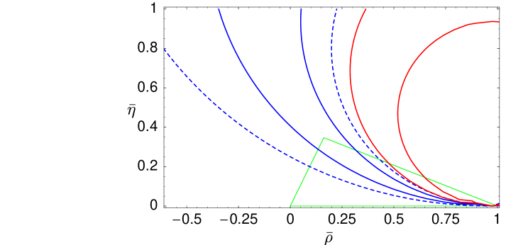
Figure 2: Constraint in the ($\bar{\rho},\bar{\eta}$) plane from $a^{d}_{\rm fs}$. Area between solid pair of curves: NLO, for the cases $a^{d}_{\rm fs}=-5\times 10^{-4}$ (left) and $a^{d}_{\rm fs}=-10^{-3}$ (right). Area between dashed curves: LO for $a^{d}_{\rm fs}=-5\times 10^{-4}$. The current best fit to the unitarity triangle $\!{}^{{\bf?}}$ is also shown.

The result for the $B_{s}$ system is

$$a_{\rm fs}^{s} = (12.0\pm 2.4)\cdot 10^{-4}\,|V_{us}|^{2}R_{t}\sin\beta\;=\;(2.1\pm 0.4)\cdot 10^{-5}.$$

From Eq. (7) one finds that $\Delta\Gamma_{q}/\Delta M_{q}=-{\rm Re}(\Gamma_{12}^{q}/M_{12}^{q})$. This ratio was predicted to NLO in $\!{}^{{\bf?}}$ for the $B_{s}$ system. With the new result of $\!{}^{{\bf?},{\bf?}}$ we can also predict $\Delta\Gamma_{d}/\Delta M_{d}$. Due to a numerical accident, the Standard Model prediction for the ratio $\Delta\Gamma_{q}/\Delta M_{q}$ is essentially the same for $q=d$ and $q=s$:

$$\frac{\Delta\Gamma_{q}}{\Delta M_{q}}=(4.0\pm 1.6)\times 10^{-3}\,,\qquad\qquad\frac{\Delta\Gamma_{d}}{\Gamma_{d}}=(3.0\pm 1.2)\times 10^{-3}.$$ (21)

The precise values for the quark masses, “bag” factors and $\alpha_{s}$ used for our numerical predictions can be found in Eq. (7) of $\!{}^{{\bf?}}$.

We close our discussion with a remark about the $B_{s}$ system. It is possible that new physics contributions render the $B_{s}\!-\!\,\overline{\!B}{}_{s}\,$ oscillations so large that a measurement of $\Delta M_{s}$ will be impossible. In general such new physics contribution will affect the CP phase $\phi_{s}$ and suppress $\Delta\Gamma_{s}$ in Eq. (7). Different measurements of $\Delta\Gamma_{s}$ can then determine $|\cos\phi_{s}|$ despite of the unobservably rapid $B_{s}\!-\!\,\overline{\!B}{}_{s}\,$ oscillations $\!{}^{{\bf?}}$. A measurement of the sign of $a_{\rm fs}^{s}\propto\sin\phi_{s}$ (which will then be enhanced, unless $\Delta M_{s}$ is extreme) through e.g. Eq. (17) will then reduce the four-fold ambiguity in $\phi_{s}$ from the measurement of $|\cos\phi_{s}|$ to a two-fold one.

References

References

- [1] K. Anikeev et al., physics at the Tevatron: Run II and beyond, [hep-ph/0201071], Chapters 1.3 and 8.3.
- [2] E. H. Thorndike, Ann. Rev. Nucl. Part. Sci. 35 (1985) 195; J. S. Hagelin and M. B. Wise, Nucl. Phys. B 189 (1981) 87; J. S. Hagelin, Nucl. Phys. B 193 (1981) 123; A. J. Buras, W. Slominski and H. Steger, Nucl. Phys. B 245 (1984) 369.
- [3] R. N. Cahn and M. P. Worah, Phys. Rev. D 60 (1999) 076006; S. Laplace, Z. Ligeti, Y. Nir and G. Perez, Phys. Rev. D 65 (2002) 094040.
- [4] O. Schneider, mixing, hep-ex/0405012, to appear in S. Eidelman et al. (Particle Data Group), Review of Particle Physics.
- [5] A. J. Buras, M. Jamin and P. H. Weisz, Nucl. Phys. B 347 (1990) 491.
- [6] M. Beneke, G. Buchalla, C. Greub, A. Lenz and U. Nierste, Phys. Lett. B 459 (1999) 631.
- [7] M. Ciuchini, E. Franco, V. Lubicz, F. Mescia and C. Tarantino, JHEP 0308, 031 (2003).
- [8] M. Beneke, G. Buchalla, A. Lenz and U. Nierste, Phys. Lett. B 576 (2003) 173.
- [9] M. A. Shifman and M. B. Voloshin, in: Heavy Quarks ed. V. A. Khoze and M. A. Shifman, Sov. Phys. Usp. 26 (1983) 387; M. A. Shifman and M. B. Voloshin, Sov. J. Nucl. Phys. 41 (1985) 120 [Yad. Fiz. 41 (1985) 187]; M. A. Shifman and M. B. Voloshin, Sov. Phys. JETP 64 (1986) 698 [Zh. Eksp. Teor. Fiz. 91 (1986) 1180]; I. I. Bigi, N. G. Uraltsev and A. I. Vainshtein, Phys. Lett. B 293 (1992) 430 [Erratum-ibid. B 297 (1992) 477].
- [10] M. Beneke, G. Buchalla and I. Dunietz, Phys. Rev. D 54 (1996) 4419. A. S. Dighe, T. Hurth, C. S. Kim and T. Yoshikawa, Nucl. Phys. B 624 (2002) 377.
- [11] M. Battaglia et al., The CKM matrix and the unitarity triangle, [hep-ph/0304132].
- [12] Y. Grossman, Phys. Lett. B380 (1996) 99. I. Dunietz, R. Fleischer and U. Nierste, Phys. Rev. D 63 (2001) 114015.