BU-HEPP-03/12, UTHEP-03-1201
Dec. 2003

Comparisons of Fully Differential Exact Results for ${\cal O}(\alpha)$ Virtual Corrections to Single Hard Bremsstrahlung in $e^{+}e^{-}$ Annihilation at High Energies^†

C.Glosser^a,b,c, S. Jadach^d,e, B.F.L. Ward^a and S.A. Yost^a
aDepartment of Physics,
Baylor University, Waco, Texas 76798-7316, USA
^bDepartment of Physics and Astronomy,
The University of Tennessee, Knoxville, Tennessee 37996-1200, USA
^cDepartment of Physics,
Southern Illinois University, Edwardsville, IL 62026-1654, USA
^dCERN, Theory Division, CH-1211 Geneva 23, Switzerland,
^eInstitute of Nuclear Physics, ul. Radzikowskiego 152, Kraków, Poland,

Abstract

We present comparisons of the fully differential exact virtual correction to the important single hard bremsstrahlung process in $e^{+}e^{-}$ annihilation at high energies , which is essential for precision studies of the Standard Model from 1 GeV to 1 TeV, as calculated by two completely independent methods and groups. We show that the two sets of results are in excellent agreement. Phenomenological implications are discussed.

• Work partly supported by the US Department of Energy Contract DE-FG05-91ER40627 and by NATO grant PST.CLG.980342.

Now that the Standard Model electroweak theory has been established at the one-loop level [1, 2], the stage is set for studying its consequences as both signal and background to the physics objectives of current and planned high energy colliding beam devices, from 1 GeV to 1 TeV for the cms energy in $e^{+}e^{-}$ annihilations for example. The attendant per mille level studies necessitate control of the EW higher order radiative corrections at least to order ${\cal O}(\alpha^{3}L^{3})$ for the leading log effects and to the exact ${\cal O}(\alpha^{2})$. One set of the important contributions to the latter exact results are the virtual corrections to the single hard bremsstrahlung in $e^{+}e^{-}$ annihilations, which therefore have been studied by several groups [3, 4, 5, 6]. Comparisons of these results are essential in order to gain some confidence in their correctness and some facility in their use to confront the SM with precision data. For example, in the effort to exploit the radiative return from cms energies in the 1-2 GeV regime to the resonance regime of the $\pi\pi$ system in the Daphne environment, precision predictions of the type compared in this paper are essential. Similarly, in order to use the radiative return from 200 GeV to the Z in the final LEPII data analysis for precision EW tests, again precision predictions of the type compared in the following for the respective return processes are essential.

Indeed, in Refs. [5], some of us (S.J., B.F.L.W., S.A.Y.) have presented comparisons of the results in Refs. [3, 4, 5] and in general a very good agreement was found. However, if one looks at the comparisons in Ref. [5], one can see that at the level of the NNLL (next-to-next leading log), there was a difference in the results that was consistent with the different levels of “exactness” in the calculations. Specifically, the mass corrections are included in Ref. [5] in a fully differential way, whereas in Ref. [3] the mass corrections are included but the photon angular variable is integrated over and in Ref. [4] the results are fully differential but the mass corrections are incomplete. These comparisons therefore can not really test the NNLL, fully differential results in Ref. [5].

The situation has changed recently with the advent for the results of Ref. [6]. Using a completely independent method and calculation, the authors in Ref. [6] have also achieved a fully differential, exact ${\cal O}(\alpha^{2})$ result for the virtual correction to single hard bremsstrahlung in the initial state radiation in high energy $e^{+}e^{-}$ annihilation, with particular emphasis on the 1-2 GeV cms energy regime. This then affords a detail cross check at the NNLL level of the corresponding results. These comparisons are the subject of this paper.

We note that, already in Ref. [7], a preliminary indirect comparison of the results in Refs. [5, 6] has been reported via comparison of the two Monte Carlo’s PHOKHARA [6] and ${\cal KK}$ MC [8], as these two Monte Carlo’s have the realizations of the results in Ref. [6] (PHOKHARA) and Ref. [5] ( ${\cal KK}$ MC). Agreement at the per mille level was found on selected observables. This is a good basis upon which to view the results which follow.

Figure 1: Feynman graphs for the virtual ${\cal O}(\alpha)$ correction to the process $e^{+}e^{-}\rightarrow 2f+\gamma$ are illustrated, where $f\neq e$.

Specifically, the Feynman graphs under discussion are illustrated in Fig. 1. In Ref. [5] the respective ISR matrix element is evaluated using the CALKUL/Xu et al./Kleiss-Stirling [9, 10, 11] method for the attendant helicity amplitudes using FORM [12] techniques. The mass corrections are then added following the methods in Ref. [13], after checking that the exact expression for the mass corrections differs from the result obtained by the latter methods by terms which vanish as $m_{e}^{2}/s\rightarrow 0$ where $m_{e}$ is the electron mass and s is the squared cms energy. In Refs. [6], the same ISR matrix element’s interference with the Born process is calculated in terms of Lorentz covariants in such a way that the mass effects are treated exactly. Thus, comparison of the two sets of results gives important information on the two different methods of calculation and on the two different treatments of the mass corrections.

For our studies, we will follow the development in Ref. [5] and systematically isolate, using the differential cross section , first, the the complete cross section, second, the size of the LL contributions, third, the size of the NLL contributions and finally the size of the NNLL contributions. In this way, we shall see how well the two independent fully differential calculations with completely different approaches agree. This of course will reinforce the confidence, whatever it may be, that we have in both calculations.

Specifically, for the process in Fig. 1, where $p_{1}(p_{2})$ is the four-momentum of the incoming $e^{+}(e^{-})$, respectively, and $k$ is that of the emitted real photon, we focus on the corresponding virtual correction to the single real bremsstrahlung differential cross section ${d\sigma}^{\rm ISR(1)}_{1}/dz$ where ${d\sigma}^{\rm ISR(1)}_{1}$ is defined in eq.(3.7) of Ref. [5] and where $z=s^{\prime}/s\equiv 1-v$ when $s$ is the squared cms total energy and $s^{\prime}$ is the squared final state $f\bar{f}$ system rest mass. Here, we will average over the initial fermion spins and sum over the final ones. This cross section has been computed in both Refs. [5] and in Refs. [6] when we restrict ourselves, as we do here, to the fully ISR (initial state radiation) corrections and processes. Continuing to follow the work in Refs. [5], we again note the that IR (infrared) limit of the process is known and can be determined from the arguments of Yennie, Frautschi and Suura in Ref. [14]. Thus, with an eye toward the use of the results in Refs. [5] in the YFS based CEEX (coherent exclusive exponentiated) Monte Carlo KK MC [8], we work with the cross section associated with the virtual correction to the hard photon residual $\bar{\beta}_{1}^{(1)}$ as it is defined in Refs. [14, 8] for example. This allows us to focus on the non-IR singular part of the respective cross sections.

What we find is illustrated in Figs. 2-5, for the case $f\bar{f}=\mu^{-}\mu^{+}$.

Figure 2: This is the $\bar{\beta}_{1}^{(2)}$ distribution for the YFS3ff MC (YFS3ff is the EEX3 matrix element option of the ${\cal KK}$ MC in Ref. [8]), as a function of energy cut $v_{\max}$. It is divided by the Born cross-section. The exact and NLL results from Ref. [5] are compared to the IN result from Ref. [4], the BVNB result from Ref. [3], and the KR result from Ref. [6].

In Fig. 2, we show the complete $\bar{\beta}_{1}^{(2)}$ distribution for our exact result and our NLL approximate results as presented in Ref. [5], the result of Igarashi and Nakazawa et al. [4], the result of Berends et al. [3], and, what is new here, the exact result of Kuhn and Rodrigo in Ref. [6]. What we see is that there is a very good general agreement between all of these results. To better assess the difference between them, we plot in Fig. 3 the difference between the respective ${\cal O}(\alpha^{2})$ and ${\cal O}(\alpha^{1})$ results. Again we see very good agreement between the results.

Figure 3: Difference $\bar{\beta}_{1}^{(2)}-\bar{\beta}_{1}^{(1)}$ for the YFS3ff MC (the EEX3 option in the ${\cal KK}$ MC), as a function of the cut $v_{\max}$. It is divided by the Born cross-section. The comparisons are the same as in Fig. 2.

To isolate the respective predictions for the NLL effect, we plot in Fig. 4 the respective differences between our LL ${\cal O}(\alpha^{2})$ result from Ref. [5] and the other five results. The results are still essentially indistinguishable at this level, except that NLL effects become apparent in the last data point, for $v=0.9875$.

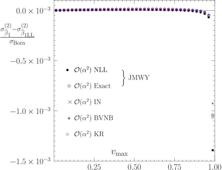
Figure 4: Next-to-leading-log contribution $\bar{\beta}_{1}^{(2)}-\bar{\beta}^{(2)}_{1\rm LL}$ for the YFS3ff MC (the EEX3 option of the ${\cal KK}$ MC), as a function of the cut $v_{\max}$. It is divided by the Born cross-section. The comparisons are the same as in Fig. 2.

These comparisons are more evident in the following graphs, Fig. 5 and Fig. 6, where we isolate the size of the four NNLL results by subtracting our NLL result from Ref. [5] from each of the results. Fig. 6 is identical to Fig. 5, except for the scale, which permits a closer comparison of the NLL results below a cut of 0.95, while omitting some off-scale data points beyond that cut. It was already established in Ref. [5] that the expressions of Ref. [4] and Ref. [3] agree analytically with our NLL upon taking a collinear photon limit. This has been checked as well for the massless limit of the result of Ref. [6].

In the NNLL comparisons, all of the results agree to within $0.4\times 10^{-5}$ for cuts below 0.75. For cuts between 0.75 and .95, the results agree to within $0.5\times 10^{-5}$, if the result of Ref. [3] is not included, and within $1.1\times 10^{-5}$ if that result is included. For the last data point, at $v=0.9875$, the result of Ref. [3] is approximately $1\times 10^{-4}$ greater than the others, while the remaining results agree to $3\times 10^{-5}$.

These results are consistent with a total precision tag of $1.5\times 10^{-5}$ for our ${\cal O}(\alpha^{2})$ correction $\bar{\beta}_{1}^{(2)}$ for an energy cut below $v=0.95$. The NLL effect alone is adequate to within $1.5\times 10^{-5}$ for cuts below 0.95. The NLL effect has already been implemented in the ${\cal KK}$ MC in Ref. [8] and the attendant version of KK MC will be available in the near future [15].

Figure 5: Sub-NLL contribution $\bar{\beta}_{1}^{(2)}-\bar{\beta}^{(2)}_{1\rm NLL}$ for the YFS3ff MC (the EEX3 option of the ${\cal KK}$ MC), as a function of the cut $v_{\max}$. It is divided by the Born cross-section. The comparisons are the same as in Fig. 2.

Figure 6: Sub-NLL contribution $\bar{\beta}_{1}^{(2)}-\bar{\beta}^{(2)}_{1\rm NLL}$ with an expanded scale to show clearly the differences in the NNLL results for cuts up to 0.95.

We have also made the analogous study to Figs. 2-5 for 500 GeV. We find very similar results, with the total precision tag of $2\times 10^{-4}$.

In this paper, we have presented new comparisons of exact results for the virtual correction to the process $e^{+}e^{-}\rightarrow f\bar{f}+\gamma$ for the ISR. The results from Ref. [5] are already in use in the ${\cal KK}$ MC in Ref. [8] in connection with the final LEP2 data analysis.

We have compared our results with those in Refs. [4, 3, 6] and in general we find very good agreement, both at 200 GeV and at 500 GeV. The comparisons with the results in Ref. [6], which like our results in Ref. [5] are exact but which have the complete mass corrections included explicitly whereas our mass corrections are included using the approach of Ref. [13] ( which we have shown to differ from the exact mass results by terms which vanish as $m_{e}^{2}/s\rightarrow 0$ ), allow us to lower our precision tag to $1.5\times 10^{-5}$ for an energy cut below 0.95 compared to what we quoted in Ref. [5]. For example, the size of the NNLL correction is now shown to be at or below the level of $1.5\times 10^{-5}$ for all values of the energy cut parameter up to 0.95.

We need to stress that a considerable amount of simplification of large cancelling terms in the expressions in Refs. [5, 6] was required to produce the results in this paper. Only after all such cancellations were found and carried out analytically could the agreement shown in Figs. 2-6 be realized. The details of this part of the analysis will appear elsewhere [15].

Our results are fully differential and are therefore ideally suited for MC event generator implementation. This has been done in the ${\cal KK}$ MC in Ref. [8]. The results from Ref. [6] are also fully differential with mass corrections and have also been fully implemented into a Monte Carlo event generator [6], albeit one without YFS exponentiation. It is therefore natural to compare the two respective event generators in the context of the radiative return at $\Phi$ and B-factories. As we noted above, a preliminary version of such results already appeared in Ref. [7], where per mille level agreement was found. The results above indicate that, in principle, much better agreement is possible. Further such comparisons will appear elsewhere [15].

What one sees from the comparisons above is that we now have a firm handle on the precision tag for an important part of the complete ${\cal O}(\alpha^{2})$ corrections to the $2f$ production process needed for precision studies of such processes in the final LEP2 data analysis, in the radiative return at $\Phi$ and B-Factories, and in the future TESLA/LC physics.

References

- [1] S.L. Glashow, Nucl. Phys. 22 (1961) 579; S. Weinberg, Phys. Rev. Lett. 19 (1967) 1264; A. Salam, in Elementary Particle Theory, ed. N. Svartholm (Almqvist and Wiksells, Stockholm, 1968), p. 367; G. ’t Hooft and M. Veltman, Nucl. Phys. B44,189 (1972) and B50, 318 (1972); G. ’t Hooft, ibid. B35, 167 (1971); and M. Veltman, ibid. B7, 637 (1968).
- [2] D. Abbaneo et al., hep-ex/0212036; see also, M. Gruenewald, hep-ex/0210003, in Proc. ICHEP02, in press, 2003.
- [3] F.A. Berends, W.L. Van Neerven and G.J.H. Burgers, Nucl. Phys. B297 (1988) 429 and references therein.
- [4] M. Igarashi and N. Nakazawa, Nucl. Phys. B288 (1987) 301.
- [5] S. Jadach, M. Melles, B.F.L. Ward and S.A. Yost, Phys. Rev. D65 (2002) 073030.
- [6] H. Kuhn and G. Rodrigo, Eur.Phys.J. C25 (2002) 215; H. Czyz, A. Grzelinska, J.H. Kuhn and G. Rodrigo, Eur.Phys.J. C33 (2004) 333.
- [7] H. Czyz, A. Grzelinska, J.H. Kuhn and G. Rodrigo, hep-ph/0312217.
- [8] S. Jadach, B.F.L. Ward and Z. Wa̧s, Phys. Rev. D63 (2001) 113009; Comput. Phys. Commun. 130 (2000) 260; and references therein.
- [9] F.A. Berends, P. De Causmaecker, R. Gastmans, R. Kleiss, W. Troost and T.T. Wu, Nucl. Phys. B264 (1986) 243, 265.
- [10] Z. Xu, D.-H. Zhang and L. Chang, Nucl. Phys. B291 (1987), 392.
- [11] R. Kleiss and W.J. Stirling, Nucl.Phys. B262 (1985) 235; Phys. Lett. B179 (1986) 159.
- [12] J.A.M. Vermaseren, The symbolic manipulation program FORM, versions 1-3, available via anonymous FTP from nikhefh.nikhef.nl.
- [13] F. A. Berends et al., Nucl. Phys. B206 ( 1982 ) 61.
-
[14]
D. R. Yennie, S. C. Frautschi, and H. Suura, Ann. Phys. 13 (1961) 379;
see also K. T. Mahanthappa, Phys. Rev. 126 (1962) 329, for a related analysis. - [15] S. Jadach et al, to appear.