Are solar neutrino oscillations robust?

Abstract:

The robustness of the large mixing angle (LMA) oscillation (OSC) interpretation of the solar neutrino data is considered in a more general framework where non-standard neutrino interactions (NSI) are present. Such interactions may be regarded as a generic feature of models of neutrino mass. The 766.3 ton-yr data sample of the KamLAND collaboration are included in the analysis, paying attention to the background from the reaction ${}^{13}C(\alpha,n)^{16}O$. Similarly, the latest solar neutrino fluxes from the SNO collaboration are included. In addition to the solution which holds in the absence of NSI (LMA-I) there is a “dark-side” solution (LMA-D) with $\sin^{2}\theta_{\textsc{sol}}=0.70$, essentially degenerate with the former, and another light-side solution (LMA-0) allowed only at 97% CL. More precise KamLAND reactor measurements will not resolve the ambiguity in the determination of the solar neutrino mixing angle $\theta_{\textsc{sol}}$, as they are expected to constrain mainly $\Delta m^{2}_{\textsc{sol}}$. We comment on the complementary role of atmospheric, laboratory (e. g. CHARM) and future solar neutrino experiments in lifting the degeneracy between the LMA-I and LMA-D solutions. In particular, we show how the LMA-D solution induced by the simplest NSI between neutrinos and down-type-quarks-only is in conflict with the combination of current atmospheric data and data of the CHARM experiment. We also mention that establishing the issue of robustness of the oscillation picture in the most general case will require further experiments, such as those involving low energy solar neutrinos.

1 Introduction

The very first data of the KamLAND collaboration eguchi:2002dm have been enough to isolate neutrino oscillations as the correct mechanism explaining the solar neutrino problem pakvasa:2003zv , indicating also that large mixing angle (LMA) was the right solution. The 766.3 ton-yr KamLAND data sample strengthens the validity of the LMA oscillation interpretation of the data Araki:2004mb .

With neutrino experiments now entering the precision age McDonald:2004dd , the determination of neutrino parameters and their theoretical impact have become one of the main goals in astroparticle and high energy physics Maltoni:2004ei . Now the main efforts should be devoted to the precision determination of the oscillation parameters and to test for sub-leading non-oscillation effects such as spin-flavour conversions schechter:1981hw , akhmedov:1988uk or non-standard neutrino interactions (NSI, for short) Wolfenstein:1977ue .

A quantitative analysis of neutrino oscillations reveals that the interpretation is relatively robust even taking into account the possibility of solar density fluctuations in the solar radiative zone Burgess:2003su , that might arise from magnetic fields effects Burgess:2003fj , currently unconstrained by helioseismology. The robustness of neutrino oscillations in the presence of spin-flavour conversions induced by non-vanishing neutrino transition magnetic moments Miranda:2003yh follows from the stringent limit on anti-neutrinos from the Sun by the KamLAND collaboration Eguchi:2003gg  .

Here we focus on the case of neutrinos endowed with non-standard interactions. These are a natural outcome of many neutrino mass models valle:1991pk and can be of two types: flavour-changing (FC) and non-universal (NU).

Seesaw-type models leads to a non-trivial structure of the lepton mixing matrix characterizing the charged and neutral current weak interactions schechter:1980gr . This leads to gauge-induced NSI which may violate lepton flavor and CP even with massless neutrinos mohapatra:1986bd , bernabeu:1987gr , branco:1989bn , rius:1990gk , Deppisch:2004fa . Alternatively, non-standard neutrino interactions may also arise in models where neutrino masses are “calculable” from radiative corrections zee:1980ai , babu:1988ki . Finally, in some supersymmetric unified models, the strength of non-standard neutrino interactions may be a calculable renormalization effect hall:1986dx .

How sizable are non-standard interactions will be a model-dependent issue. In some models NSI strengths are too small to be relevant for neutrino propagation, because they are suppressed by some large scale and/or restricted by limits on neutrino masses. However, this need not be the case, and there are interesting models where moderate strength NSI remain in the limit of light (or even massless) neutrinos mohapatra:1986bd , bernabeu:1987gr , branco:1989bn , rius:1990gk , Deppisch:2004fa . Such may occur even in the context of fully unified models like SO(10) Malinsky:2005bi .

Non–standard interactions may in principle affect neutrino propagation properties in matter as well as detection cross sections pakvasa:2003zv . Thus their existence can modify the solar neutrino signal observed at experiments. They may be parametrized with the effective low–energy four–fermion operator:

$$\mathcal{L}_{NSI}=-\epsilon_{\alpha\beta}^{fP}2\sqrt{2}G_{F}\left(\bar{\nu}_{\alpha}\gamma_{\mu}L\nu_{\beta}\right)\left(\bar{f}\gamma^{\mu}Pf\right),$$ (1)

where P = L, R and $f$ is a first generation fermion: $e,u,d$. The coefficients $\varepsilon_{\alpha\beta}^{fP}$ denote the strength of the NSI between the neutrinos of flavours $\alpha$ and $\beta$ and the P–handed component of the fermion $f$. In the present work, for definiteness, we take for $f$ the down-type quark. However, one can also consider the presence of NSI with electrons and up and down quarks simultaneously. Current limits and perspectives in the case of NSI with electrons have been reported in the literature NSI-e .

While strong constraints exist from $\nu_{\mu}$ interactions with a down-type quark ($\varepsilon^{dP}_{e\mu}\lesssim 10^{-3}$, $\varepsilon^{dP}_{\mu\mu}\lesssim 10^{-3}-10^{-2}$) from CHARM and NuTeV Davidson:2003ha , the constraints for all other NSI couplings, including those involved in solar neutrino physics, are rather loose Davidson:2003ha , Berezhiani:2001rs . Therefore, in our analysis we consider $\varepsilon_{\alpha\mu}^{dP}=0$ and we concentrate our efforts in the rest of NSI parameters.

For our solar neutrino analysis, we will consider the simplest approximate two–neutrino picture, which is justified in view of the stringent limits on $\theta_{13}$ Maltoni:2004ei that follow mainly from reactor neutrino experiments apollonio:1999ae .

The Hamiltonian describing solar neutrino evolution in the presence of NSI contains, in addition to the standard oscillations term

$$\left(\begin{array}[]{lc}-\frac{\Delta m^{2}}{4E}\cos 2\theta+\sqrt{2}\,G_{F}N_{e}\nobreak\leavevmode\nobreak\leavevmode&\frac{\Delta m^{2}}{4E}\sin 2\theta\\ \leavevmode\nobreak\ \leavevmode\nobreak\ \leavevmode\nobreak\ \frac{\Delta m^{2}}{4E}\sin 2\theta&\frac{\Delta m^{2}}{4E}\cos 2\theta\end{array}\right)$$ (2)

a term $H_{\mathrm{NSI}}$, accounting for an effective potential induced by the NSI with matter, which may be written as:

$$H_{\mathrm{NSI}}=\sqrt{2}G_{F}N_{d}\left(\begin{array}[]{cc}0&\varepsilon\\ \varepsilon&\varepsilon^{\prime}\end{array}\right)\,.$$ (3)

Here $\varepsilon$ and $\varepsilon^{\prime}$ are two effective parameters that, according to the current bounds discussed above ($\varepsilon_{\alpha\mu}^{fP}\sim 0$), are related with the vectorial couplings which affect the neutrino propagation by:

$$\varepsilon=-\sin\theta_{23}\,\varepsilon_{e\tau}^{dV}\qquad\varepsilon^{\prime}=\sin^{2}\theta_{23}\,\varepsilon_{\tau\tau}^{dV}-\varepsilon_{ee}^{dV}$$ (4)

The quantity $N_{d}$ in Eq. (3) is the number density of the down-type quark along the neutrino path. In the more general case, the effective couplings $\varepsilon$ and $\varepsilon^{\prime}$ will contain contributions from the three fundamental fermions and NSI effects would be important not only in neutrino propagation but also in the detection process.

It is important to note that the neutrino evolution inside the Sun and the Earth is sensitive only to the vector component of the NSI, $\varepsilon_{\alpha\beta}^{dV}=\varepsilon_{\alpha\beta}^{dL}+\varepsilon_{\alpha\beta}^{dR}$. The effect of the axial coupling will be discussed in detail in section 4.

Before introducing our numerical analysis of the solar neutrino data in the next section, it is worth discussing the analytical formulas for neutrino survival probability in the constant matter density case, in order to have a better understanding of the results that will be shown in the next section. Recall first that in two–neutrino oscillations deGouvea:2000cq , Gonzalez-Garcia:2000cm one can, without loss of generality, restrict the variation of the mixing angle $\theta$ only to the range $[0,\frac{\pi}{2}]$ and still cover the whole physical space . In the adiabatic regime the survival probability can be approximated by Parke’s formula Parke:1986jy

$$P(\nu_{e}\to\nu_{e})=\frac{1}{2}\left[1+\cos 2\theta\cos 2\theta_{m}\right],$$ (5)

where $\theta_{m}$ is the effective mixing angle at the neutrino production point inside the sun. In the absence of non-standard neutrino–matter interactions the mixing angle in matter may be obtained from the expression

$$\cos 2\theta_{m}=\frac{\Delta m^{2}\cos 2\theta-2\sqrt{2}\,EG_{F}N_{e}}{\sqrt{\left(\Delta m^{2}\cos 2\theta-2\sqrt{2}\,EG_{F}\,N_{e}\right)^{2}+\left(\Delta m^{2}\sin 2\theta\right)^{2}}}\,,$$ (6)

In order to explain the deficit of solar neutrinos observed at the detectors, the neutrino survival probability should satisfy: $P<0.5$. According to Eqs. (5) and (6), this requirement is not satisfied for $\cos 2\theta<0$, so that only vacuum mixing angles in the “light side” ($0<\theta<\frac{\pi}{4}$) can give solution to the solar neutrino problem. Indeed this is confirmed by the results shown in Fig. 1.

Lets now turn to the case where non-standard interactions are present, in addition to oscillations. Within such generalized picture (OSC+NSI), Eq. (6) is modified to

$$\cos 2\theta_{m}=\frac{\Delta m^{2}\cos 2\theta-2\sqrt{2}\,EG_{F}(N_{e}-\varepsilon^{\prime}N_{d})}{\left[\Delta m^{2}\right]_{matter}},$$ (7)

where

$$\left[\Delta m^{2}\right]_{matter}^{2}=\left[\Delta m^{2}\cos 2\theta-2\sqrt{2}\,EG_{F}(N_{e}-\varepsilon^{\prime}N_{d})\right]^{2}\\ +\left[\Delta m^{2}\sin 2\theta+4\sqrt{2}\,\varepsilon\,EG_{F}N_{d}\right]^{2}$$ (8)

Thanks to the presence of the non-universal coupling $\varepsilon^{\prime}$ one can obtain $P<0.5$ even for $\cos 2\theta<0$ as long as $\varepsilon^{\prime}>\frac{2\sqrt{2}\,EG_{F}N_{e}+\Delta m^{2}|\cos 2\theta|}{2\sqrt{2}\,EG_{F}N_{d}}$. This makes it possible to explain the solar neutrino data for values of the vacuum mixing angle in the dark side, for large enough values of $\varepsilon^{\prime}$. As we will see below this possibility will lead to the appearance of the LMA-D solution with $\theta>\frac{\pi}{4}$ and thus to the ambiguous determination of the solar mixing angle.

2 The fit

Here we reanalyse the robustness of the oscillation interpretation of the solar neutrino data in the presence of non–standard interactions. We include the recent SNO data Aharmim:2005gt as well as the 766.3 ton-yr data sample from the KamLAND collaboration Araki:2004mb , taking into account the background from the reaction ${}^{13}C(\alpha,n)^{16}O$. In order to do this we first calibrate with the results obtained in the pure oscillation case for the KamLAND–only, solar–only and combined data samples. For the KamLAND analysis we use a Poisson statistics as described in Fogli:2002au . Our best fit point is located at $\sin^{2}2\theta_{\textsc{sol}}=0.84$ and $\Delta m^{2}_{\textsc{sol}}=7.9\times 10^{-5}$ eV ², in good agreement with the results of Ref. Araki:2004mb . For the solar data we include the rates for the Chlorine, Gallex/GNO, SAGE, as well as the Super-Kamiokande spectrum, SNO day/night spectrum and SNO salt data, with a total of 84 observables. We adopt the pull method Fogli:2002pt to fit the data using the most recent BS05 Standard Solar Model Bahcall:2004pz . We perform a complete analysis of the solar neutrino data using a numerical computation for the survival probabilities both in the light as well as in the dark side of the mixing angle, for values of $\Delta m^{2}_{\textsc{sol}}$ in the range of $10^{-6}$ to $10^{-3}$ eV² and running also both $\varepsilon$ and $\varepsilon^{\prime}$ at the same time in the range $[-1,1]$. Our results for $\varepsilon=\varepsilon^{\prime}=0$ are shown in Fig. 1.

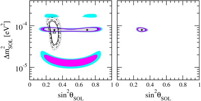
Figure 1: 90%, 95%, 99% and 99.73% C.L. allowed regions of the neutrino oscillation parameters from the analysis of the latest solar data (hollow lines, left panel), and latest KamLAND data (colored regions, left panel) and from the combined analysis (right panel).

The best fit point for this global analysis is given by $\sin^{2}\theta_{\textsc{sol}}=0.29$ and $\Delta m^{2}_{\textsc{sol}}=8.1\times 10^{-5}$ eV ². This is in excellent agreement with the results obtained in Maltoni:2004ei for the solar case. Reassured by this calibration we now turn to the generalized OSC+NSI picture.

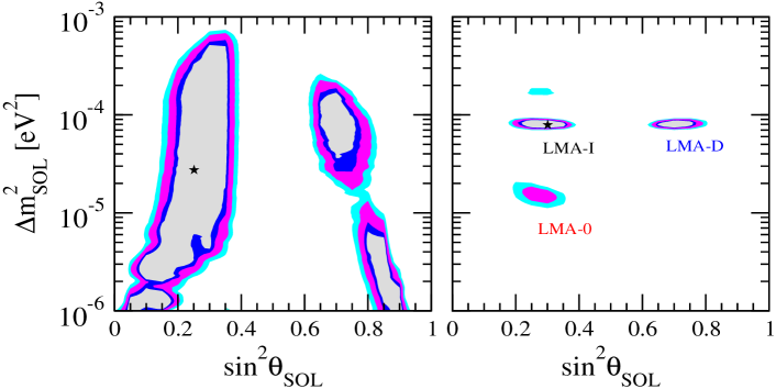
Figure 2: Allowed regions for the generalized OSC + NSI case, determined from the latest data: left panel corresponds to a solar only analysis, while the right panel corresponds to the combined solar+KamLAND analysis.

Our results for this case are shown in Fig. 2 and Table 1.

	$\sin^{2}\theta_{\textsc{sol}}$	$\Delta m^{2}_{\textsc{sol}}$ [eV2]	$\varepsilon$	$\varepsilon^{\prime}$	$\chi^{2}$
OSC analysis
LMA-I	0.29	8.1$\times$10-5	–	–	79.9
OSC+NSI analysis
LMA-I	0.30	7.9$\times$10-5	0	-0.05	79.7
LMA-D	0.70	7.9$\times$10-5	-0.15	-0.90	80.2
LMA-0	0.25	1.6$\times$10-5	-0.10	-0.30	86.8

Table 1: Best fit solar neutrino oscillation points with and without non-standard neutrino interactions.

One sees that, in the light side, we obtain a region of allowed oscillation parameters larger than in the pure oscillation case, but more restricted than those obtained in previous OSC+NSI analysis of Refs. Friedland:2004pp , Guzzo:2004ue due to the effect of the recent KamLAND data, visible mainly in $\Delta m^{2}_{\textsc{sol}}$. The table gives the parameter best fit values for the OSC and OSC+NSI fits. For the OSC+NSI analysis the best fit occurs for $\varepsilon=0.0$ and $\varepsilon^{\prime}=-0.05$. Clearly the quality of the fit obtained with and without NSI is comparable, as seen from the $\chi^{2}$ values given in the last column of the table. The most remarkable result is, however, the appearance of an additional solution in the dark side region, which can be qualitatively understood from the discussion given at the end of Sect. 1. This LMA-D solution has $\sin^{2}\theta_{\textsc{sol}}=0.70$ and the same $\Delta m^{2}_{\textsc{sol}}$ value as the LMA-I solution and is significantly better than the LMA-0 OSC+NSI solution of Ref. Friedland:2004pp , Guzzo:2004ue , as shown in the table. On the other hand, it is nearly degenerate with the LMA-I solution, as seen by the $\chi^{2}$ value. This solution is characterized by $\varepsilon^{\prime}=0.90$, although lower values $\sim$ 0.75 are allowed at 3$\sigma$. Although embarrassingly large, one sees that such large NSI strength values are perfectly compatible with all existing solar and reactor neutrino data, including the small values of the neutrino masses indicated by current oscillation data. This opens a potentially physics challenge for upcoming low energy solar neutrino experiments, such as Borexino. Note that large NSI values could affect also solar neutrino detection, as considered in Berezhiani:2001rt . In what follows we give a discussion of the role of other experiments in probing neutrino properties at the level implied by the above LMA-D solution.

3 Constraints on NSI: present and future

As we just saw there are constraints on non-standard neutrino interaction strength parameters that follow from current solar and KamLAND data. The existence of NSI could also potentially affect neutrino-nucleon scattering and there are laboratory data that potentially constrain their allowed strength. Moreover, one must check restrictions that follow from atmospheric data. Here we discuss their complementarity.

3.1 Solar and KamLAND

We can derive limits on NSI parameters from solar and KamLAND data by displaying our $\chi^{2}$ as a function of the NSI parameters $\varepsilon$ or $\varepsilon^{\prime}$ and marginalizing with respect to the remaining three parameters.

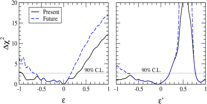
Figure 3: Constraining NSI parameters: dependence of $\Delta\chi^{2}$ with respect to $\varepsilon$ and $\varepsilon^{\prime}$, illustrating the current limits.

Figure 3 gives the $\Delta\chi^{2}$ profiles with respect to $\varepsilon$ and $\varepsilon^{\prime}$. From here one can determine the corresponding constraints on $\varepsilon$ and $\varepsilon^{\prime}$. We can see that at 90% C.L. $-0.93\leq\varepsilon\leq 0.30$ while for $\varepsilon^{\prime}$ the only forbidden region is $[0.20,0.78]$. Note that our limits on $\varepsilon^{\prime}$ are weaker than those of Ref. Guzzo:2004ue , which apply only to the restricted case where $\varepsilon=0$. We see that the limits on the strength of non-standard neutrino interactions are still very poor. The dashed lines in Fig. 3 denote the ultimate reach of this method of constraining NSI parameters (through their effect in solar neutrino propagation), namely they correspond to the case where solar neutrino oscillation parameters $\Delta m^{2}_{\textsc{sol}}$ and $\theta_{\textsc{sol}}$ are determined with infinite precision. One sees that in this ideal case the allowed range narrows down mainly for negative NSI parameter values. We conclude that there is substantial room still left for sub–leading non-standard neutrinos conversions in matter and, moreover, that the determination of solar neutrino oscillation parameters, especially the solar mixing angle, is currently ambiguous. It is unlikely that more precise reactor measurements by KamLAND will resolve this mixing angle ambiguity, as they are expected to constrain mainly $\Delta m^{2}_{\textsc{sol}}$.

In Fig. 4 we present the predicted neutrino survival probabilities versus energy, from the region of pp neutrinos up to the high energy solar neutrinos, for the three best–fit points of the allowed regions found above. One sees that the solutions predict different rates for the low energy neutrinos (e.g. pp and pep), so that future low energy solar neutrino experiments may have a hope of disentangling these solutions. Similarly, in the region of boron neutrinos our LMA-D solution also predicts a distortion in the spectrum that might be detectable at future water Cerenkov experiments such as UNO or Hyper-K UNO , given the high statistics expected. With good luck such high statistics experiments may have a window of opportunity.

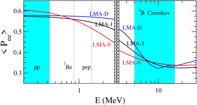
Figure 4: Predicted neutrino survival probability for low-energy neutrinos (left) and boron neutrinos (right) at the best fit points of LMA-I, LMA-D and LMA-0.

3.2 Laboratory experiments

The laboratory bounds on the neutrino non-standard interactions with down-type quarks can be summarized as $|\varepsilon_{\tau e}^{dP}|<0.5$, $|\varepsilon_{\tau\tau}^{dR}|<6$, $|\varepsilon_{\tau\tau}^{dL}|<1.1$, $-0.6<\varepsilon_{ee}^{dR}<0.5$, $-0.3<\varepsilon_{ee}^{dL}<0.3$  , see e. g. Ref Davidson:2003ha . Here we are interested in vector-like NSI couplings. For the case of $\varepsilon_{ee}^{dV}$, these bounds can be translated to $-0.5<\varepsilon_{ee}^{dV}<1.2$, while for $\varepsilon_{\tau\tau}^{dV}$ one finds a much wider range. However, we stress that these bounds have been obtained assuming that only one parameter is effective at a time. Relaxing this assumption opens more freedom. This is why we have chosen to indicate them by the dashed lines in Fig. 5. Assuming maximal mixing in the 2–3 sector in Eq. (4), one has

$$\varepsilon=-0.15 \to \varepsilon_{e\tau}^{dV}=0.21$$ (9)

$$\varepsilon^{\prime}=\hphantom{-}0.90 \to \varepsilon_{\tau\tau}^{dV}=2\leavevmode\nobreak\ (\varepsilon_{ee}^{dV}+0.90)$$ (10)

¿From this one can see explicitly that, even taking the above constraints at face value, they still leave room for our degenerate dark-side solution with $\varepsilon^{\prime}=0.90$.

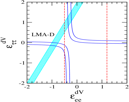
Figure 5: Consistency between the $\varepsilon^{\prime}$ coupling required for our LMA-D solution (shaded band) and the regions allowed by atmospheric data in the analytic approximation of Ref. Friedland:2004ah for $\varepsilon_{e\tau}^{dV}=0.21$ (solid lines). The laboratory constraints are also shown (dashed lines). See the text for a detailed explanation.

3.3 Atmospheric data

Concerning the atmospheric neutrino data, it is known that a large NSI strengths can originate a suppression of the neutrino oscillation amplitude. This has indeed been used in a two-neutrino analysis Fornengo:2001pm in order to obtain relatively strong bounds on the NSI strength. However, in a 3–neutrino analysis of atmospheric data Friedland:2004ah it has been explicitly shown that large NSI strengths are not excluded. In particular, these authors have found two specific scenarios where somewhat large NSI strengths can fit well the experimental data, because their effect will be indistinguishable from the standard oscillation case, at least at high and low energies. Adapting their definitions to our notation, and using their analytical description , we obtain the two branches indicated in Fig. 5. One sees that the shaded band corresponding to our LMA-D solution at 90% C.L. (with $\varepsilon_{e\tau}^{dV}=0.21$) intersects these branches in two disjoint regions, suggesting that, indeed, the NSI couplings required by the LMA-D solution are compatible with the atmospheric neutrino data. However, in a more complete numerical analysis of atmospheric neutrino data Friedland:2005vy , it has been shown that values of $\varepsilon_{\tau\tau}^{dV}$ in the right region are not allowed by atmospheric data: only the left disjoint region is compatible with atmospheric neutrino data. As indicated by the dashed lines in Fig. 5 one can see that $\varepsilon_{ee}^{dV}$ values in this region lie outside the range allowed by current laboratory data. This leads us to conclude that the LMA-D solution induced by the simplest non-standard interactions of neutrinos with only down-type quarks is ruled out by its incompatibility with atmospheric and laboratory data. However, one can verify that for the general case where neutrinos have other NSI couplings one can reconcile the above laboratory bounds with the parameters required by the LMA-D solution.

Finally, we comment on the magnitude of flavor–changing NSI of neutrinos. First note that direct constraints on the magnitude of these couplings do not exist. The only “bounds” mentioned in the literature are obtained from charged lepton flavor violating processes. While the constraints are very restrictive, they are theoretically fragile, to the extent that they rely on the assumption of weak SU(2) symmetry, and can therefore be avoided if one allows for SU(2) breaking. Note, however, that the magnitude of the FC neutrino NSI required for our dark–side solution is quite small. Futuristic proposals for improving these constraints with coherent neutrino scattering off nuclei have been already discussed Barranco:2005yy .

4 A comment on axial NSI couplings

Before we conclude, let us mention that, up to now we have only considered the effects of the NSI on the neutrino propagation through the Earth and solar interior. These effects appear as a result of the vectorial couplings of neutrinos with down-type quarks. An axial component of the NSI coupling could give rise to a non–standard contribution to the NC cross section detection at the SNO experiment. As already noted in Ref.Davidson:2003ha , the SNO-NC signal will be modified as:

$$\phi_{NC}\sim f_{B}(1+2\varepsilon_{A})$$ (11)

where

$$\varepsilon_{A}=-\sum_{\alpha=e,\mu,\tau}\left<P_{e\alpha}\right>_{NC}\varepsilon_{\alpha\alpha}^{dA}$$ (12)

with $\varepsilon_{\alpha\alpha}^{dA}=\varepsilon_{\alpha\alpha}^{dL}-\varepsilon_{\alpha\alpha}^{dR}$ being the couplings which enter into the effective Lagrangian. Thus, $\varepsilon_{A}$ is independent of the effective couplings $\varepsilon$ and $\varepsilon^{\prime}$ defined in Eq. (4). In the analysis performed so far we have assumed $\varepsilon_{A}=0$. This assumption is well justified due to the good agreement between the SNO NC measurement and the SSM prediction for the boron flux. However, we now relax this assumption and include the effect of the new parameter $\varepsilon_{A}$ in our analysis.

The results obtained in a generalized analysis which takes into account the presence of an non-zero axial component of the NSI (5 parameters instead of 4) are summarized in Fig. 6.

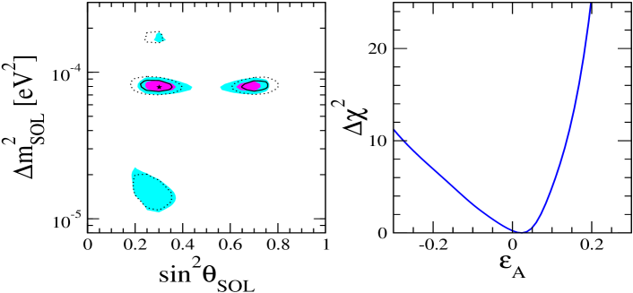
Figure 6: Results of the analysis including the axial component of the NSI. In the left panel we compare the allowed regions at 90% and 3$\sigma$ obtained with (color regions) and without (lines) $\varepsilon_{A}$. In the right panel we show the dependence of $\Delta\chi^{2}$ with respect to the axial coupling $\varepsilon_{A}$

.

One sees that the neutrino data clearly prefers $\varepsilon_{A}\sim 0$, in agreement with our previous approximation, in Sec. 2.

5 Conclusions

In short, we have reanalysed the status of the LMA oscillation interpretation of the solar neutrino data in a more general framework where non-standard neutrino interactions are present. We have seen that combining the solar neutrino data, including the latest SNO fluxes of the salt phase with the full KamLAND data sample still leaves room for a degenerate determination of solar neutrino oscillation parameters. To this extent the solar neutrino oscillation parameters extracted from the experiments may be regarded as non-robust. In addition to the lower LMA-0 solution, we have found a LMA-D solution characterized by values of the solar mixing angle larger than $\pi/4$. This solution requires large non-universal neutrino interactions on down-type quarks. While the LMA-0 solution is already disfavored, and will soon be in conflict with further data, e.g. future KamLAND reactor data, the degeneracy implied by LMA-D solution will not be resolved by more precise KamLAND reactor measurements. This shows that the determination of solar neutrino parameters only from solar and KamLAND data is not fully robust. It is crucial to consider other data samples, such as atmospheric and laboratory data, since these bring complementary information. In the present case they allow one to rule out the LMA-D solution induced by the simplest NSI between neutrinos and down-type-quarks-only, given the large values of the non–universal NSI couplings required by that solution. It is therefore important to perform similar analyses for the more general case of non-standard interactions involving electrons and/or up-type quarks. Only in such scenario (NSI with u-type, d-type and electrons) we can confidently establish the robustness of the oscillation interpretation. Further experiments, like low-energy solar neutrino experiments are therefore required in order to clear up the situation.

Work supported by Spanish grant FPA2005-01269, by European RTN network MRTN-CT-2004-503369. OGM was supported by CONACyT-Mexico and SNI. We thank Michele Maltoni and Timur Rashba for useful discussions.

References

- [1] KamLAND Collaboration, K. Eguchi et al., Phys. Rev. Lett. 90, 021802 (2003), [hep-ex/0212021].
- [2] See, for example, S. Pakvasa and J. W. F. Valle, hep-ph/0301061, Proceedings of the Indian National Academy of Sciences, Part A: Vol. 70A, No.1, p.189 - 222 (2004); V. Barger, D. Marfatia and K. Whisnant, Int. J. Mod. Phys. E 12 (2003) 56 and references therein.
- [3] KamLAND Collaboration, T. Araki, Phys. Rev. Lett. 94, 081801 (2005), [hep-ex/0406035 v3].
- [4] For a review of solar neutrino experiments see A. B. McDonald, New J. Phys. 6, 121 (2004) [astro-ph/0406253] and references therein. For latest atmospheric and K2K neutrino oscillation results see H. Gallagher, Nucl. Phys. B Proc. Suppl 143, 79 (2005). and T. Nakaya, Nucl. Phys. B Proc. Suppl 143, 196 (2005).
- [5] For a recent review see M. Maltoni, T. Schwetz, M. A. Tortola and J. W. F. Valle, New J. Phys. 6, 122 (2004). Appendix C in hep-ph/0405172 (v5) provides updated results which take into account all developments as of June 2006, namely: new SSM, new SNO salt data, latest K2K and MINOS data.
- [6] J. Schechter and J. W. F. Valle, Phys. Rev. D24, 1883 (1981), Err. Phys. Rev. D25, 283 (1982).
- [7] E. K. Akhmedov, Phys. Lett. B213, 64 (1988); C.-S. Lim and W. J. Marciano, Phys. Rev. D37, 1368 (1988).
- [8] L. Wolfenstein, Phys. Rev. D 17 (1978) 2369. S. P. Mikheev and A. Yu. Smirnov, (Editions Frontières, Gif-sur-Yvette, 1986, p.355.), 86 Massive Neutrinos in Astrophysics and Particle Physics, Proceedings of the Sixth Moriond Workshop, ed. by Fackler, O. and J. Tran Thanh Van; J. W. F. Valle, Phys. Lett. B 199 (1987) 432.
- [9] C. P. Burgess et al, JCAP 0401, 007 (2004) [hep-ph/0310366]; Astrophys. J. 588, L65 (2003) [hep-ph/0209094].
- [10] C. P. Burgess et al, Mon. Not. Roy. Astron. Soc. 348, 609 (2004) [astro-ph/0304462].
- [11] O. G. Miranda et al, Phys. Rev. D 70, 113002 (2004) [hep-ph/0406066] Phys. Rev. Lett. 93, 051304 (2004),[hep-ph/0311014].
- [12] KamLAND Collaboration, K. Eguchi et al., Phys. Rev. Lett. 92, 071301 (2004), [hep-ex/0310047].
- [13] J. W. F. Valle, Prog. Part. Nucl. Phys. 26, 91 (1991).
- [14] J. Schechter and J. W. F. Valle, Phys. Rev. D22, 2227 (1980).
- [15] R. N. Mohapatra and J. W. F. Valle, Phys. Rev. D34, 1642 (1986).
- [16] J. Bernabeu et al., Phys. Lett. B187, 303 (1987).
- [17] G. C. Branco, M. N. Rebelo and J. W. F. Valle, Phys. Lett. B225, 385 (1989).
- [18] N. Rius and J. W. F. Valle, Phys. Lett. B246, 249 (1990).
- [19] F. Deppisch and J. W. F. Valle, Phys. Rev. D 72 (2005) 036001 [hep-ph/0406040].
- [20] A. Zee, Phys. Lett. B93, 389 (1980).
- [21] K. S. Babu, Phys. Lett. B203, 132 (1988).
- [22] L. J. Hall, V. A. Kostelecky and S. Raby, Nucl. Phys. B267, 415 (1986).
- [23] M. Malinsky, J. C. Romao and J. W. F. Valle, Phys. Rev. Lett. 95 (2005) 161801 [hep-ph/0506296].
- [24] S. Pastor et al., hep-ph/0607267; A. de Gouvea and J. Jenkins, Phys. Rev. D74 033004 (2006) [hep-ph/0603036]; J. Barranco, O. G. Miranda, C. A. Moura and J. W. F. Valle, Phys. Rev. D 73 113001 (2006) [hep-ph/0512195].
- [25] S. Davidson, C. Pena-Garay, N. Rius and A. Santamaria, JHEP 0303 (2003) 011 [hep-ph/0302093].
- [26] Z. Berezhiani and A. Rossi, Phys. Lett. B 535 207 (2002) [hep-ph/0111137].
- [27] CHOOZ Collaboration, M. Apollonio et al., Phys. Lett. B466, 415 (1999), [hep-ex/9907037].
- [28] A. de Gouvea, A. Friedland and H. Murayama, Phys. Lett. B490, 125 (2000), [hep-ph/0002064].
- [29] M. C. Gonzalez-Garcia and C. Pena-Garay, Phys. Rev. D62, 031301 (2000), [hep-ph/0002186].
- [30] S. J. Parke, Phys. Rev. Lett. 57, 1275 (1986).
- [31] B. Aharmim et al. [SNO Collaboration], Phys. Rev. C 72, 055502 (2005), [nucl-ex/0502021].
- [32] G. L. Fogli et al, Phys. Rev. D 67, 073002 (2003)
- [33] G. L. Fogli, E. Lisi, A. Marrone, D. Montanino and A. Palazzo, Phys. Rev. D66, 053010 (2002), [hep-ph/0206162].
- [34] J. N. Bahcall, A. M. Serenelli and S. Basu, Astrophys. J. 621, L85 (2005) [astro-ph/0412440].
- [35] A. Friedland, C. Lunardini and C. Pena-Garay, Phys. Lett. B 594, 347 (2004) [hep-ph/0402266].
- [36] M. M. Guzzo, P. C. de Holanda and O. L. G. Peres, Phys. Lett. B591, 1 (2004), [hep-ph/0403134].
- [37] Z. Berezhiani, R. S. Raghavan and A. Rossi, Nucl. Phys. B 638, 62 (2002) [hep-ph/0111138].
-
[38]
UNO collaboration Homepage at Stonybrook:
http://superk.physics.sunysb.edu/nngroup/uno/main.html - [39] N. Fornengo, M. Maltoni, R. T. Bayo and J. W. F. Valle, Phys. Rev. D 65 (2002) 013010 [hep-ph/0108043].
- [40] A. Friedland, C. Lunardini and M. Maltoni, Phys. Rev. D 70, 111301 (2004) [hep-ph/0408264].
- [41] A. Friedland and C. Lunardini, Phys. Rev. D 72 (2005) 053009 [arXiv:hep-ph/0506143].
- [42] J. Barranco, O. G. Miranda and T. I. Rashba, JHEP 0512, 021 (2005) [arXiv:hep-ph/0508299].