Effective potential analysis for 5D SU(2) gauge theories at finite temperature and radius.

Abstract

We calculate the one loop effective potential for a 5D SU(2) gauge field theory at finite temperature $T=1/\beta$ and radius $R=1/M$. This calculation is performed, for the first time, in the case of background fields with two constant components $A^{3}_{y}$ (directed towards the compact extra dimension with radius $R$) and $A^{3}_{\tau}$ (directed towards the compact Euclidean time with radius $\beta$). This model possesses two discrete symmetries known as $Z_{M}(2)$ and $Z_{T}(2)$. The corresponding phase diagram is presented in Ref. [4]. However the arguments which lead to this diagram are mainly qualitative. We present a detailed analysis, from our point of view, for this phase diagram, and we support our arguments performing lattice simulations for a simple phenomenological model with two scalar fields interacting through the previously calculated potential.

1 Introduction

It has been noted long ago by G. ’t Hooft in Ref. [1] that a pure 4D SU(N) gauge field theory at finite temperature $T$ develops a global symmetry which is known as $Z(N)$ symmetry. In Refs. [2, 3], the one loop effective potential in the presence of a constant background gauge field $A_{0}$ was calculated. This result, which is reliable only in the weak coupling regime, implies a violation of the Z(N) symmetry. This is interpreted as the phase transition to the deconfining phase of an SU(N) gauge field theory, that is expected for high temperatures.

In recent years, there has been an interest for models with extra compact dimensions. The simplest way to extend the above model, is to add an extra compact dimension $y$ with radius $R=1/M$. As a consequence, the model develops an additional $Z(N)$ symmetry. To distinguish the two $Z(N)$ symmetries of the model, we will call $Z_{T}(N)$ the one that corresponds to the compact Euclidean time and $Z_{M}(N)$ the one that corresponds to the extra compact dimension (for details see the next section). Due to these symmetries the model possesses four distinct phases.

A schematic phase diagram (see Fig. 1 below) has been presented, for the first time, by C. P. Korthals Altes and M. Laine in Ref. [4]. However the arguments, in Ref. [4], which lead to this phase diagram are mainly qualitative. For this reason lattice simulations for a 5D and 4D SU(2) gauge field theory at finite temperature and radius were performed in Ref. [5]. The lattice results for $d=4$ confirm the phase diagram of Fig. 1. Even in the case of $d=5$ where the theory is not renormalizable, for fixed lattice spacing, the qualitative features of the above mentioned phase diagram are evident in the lattice results.

In this paper we calculate in detail the one loop effective potential for a 5D SU(2) gauge field theory at finite temperature $T$ and radius $R$. This calculation is performed in the case of background fields with two constant components $A^{3}_{y}$ and $A^{3}_{\tau}$. This result generalizes a previous calculation, in Ref. [4], for one constant gauge field component $A^{3}_{y}$ and $A^{3}_{\tau}=0$.

We will study whether it is possible to derive the qualitative features of the phase diagram of Fig. 1 by using the perturbative result for the effective potential. Unfortunately the expected restoration of the $Z_{M}(N)$ symmetry (when the system passes from region (A) to (B) in Fig. 1) for high temperature can not be established just from the effective potential. For this reason we construct a simple phenomenological model, that incorporates the fluctuations of the scalar fields, by adding to the effective potential kinetic terms. Numerical simulations on lattice for this model give a phase diagram that exhibits the main features of the expected phase diagram of Fig. 1.

2 The $Z_{T}(N)\times Z_{M}(N)$ symmetry.

The object of study, in this section, is an SU(N) gauge field theory, in a d-dimensional space-time at finite temperature, with one extra compact dimension. This extra dimension will be noted by $y$ and it varies from $0$ to $R=1/M$, where $M$ is the mass scale of Kaluza-Klein modes. In the case of finite temperature $T$ we have another compact dimension, the Euclidean time $\tau=it$, which varies from 0 to $\beta=1/T$.

The partition function of this model is:

$$Z=\int_{b.c}{\cal D}A_{\mu}e^{-\frac{1}{2}\int_{0}^{R}dy\int_{0}^{\beta}d\tau\int d^{d-2}x\;Tr\;(F_{\mu\nu})^{2}}$$ (1)

with the periodic boundary conditions

$$A_{\mu}(0,\tau,x)=A_{\mu}(R,\tau,x)$$ (2)

$$A_{\mu}(y,0,x)=A_{\mu}(y,\beta,x)$$ (3)

where $x=(x_{1},x_{2},...,x_{d-2})$. The field tensor is given by the equation $F_{\mu\nu}=\partial_{\mu}A_{\nu}-\partial_{\nu}A_{\mu}-ig_{d}[A_{\mu},A_{\nu}]$ ($\nu,\mu=1,2...d$), where $g_{d}$ is the d-dimensional coupling constant. In addition, $A_{\mu}=A^{\alpha}_{\mu}T^{\alpha}$ ( $\alpha=1,2...N^{2}-1$), and $T^{\alpha}$ satisfies the commutation relation $[T^{\alpha},T^{b}]=if^{abc}T^{c}$. Also note that for the components $A_{d-1}$ and $A_{d}$ of the gauge field we will use the notation $A_{\tau}$ and $A_{y}$.

We would like to emphasize that this action, if $d\geq 5$ (in this work we will study the case of $d=5$), corresponds to a non renormalizable field theory. However this theory is viewed as an effective theory valid up to a finite cut-off $\Lambda$, and describes the low energy behavior of a fundamental renormalizable field theory, which may be a string theory. In this way all the observables of this model are rendered finite. We note that an observable like the one-loop effective potential, which is computed in the next section, is finite and cut-off independent. Also we note that the scale $\Lambda$ is assumed to be much larger than the temperature $T$ and the mass scale $M$ (or $T<<\Lambda$ and $M<<\Lambda$). An extensive discussion on this topic is presented by K. R. Dienes et al in Ref. [6].

The action of this model is invariant under Gauge transformations

$$A^{\prime}_{\mu}=UA_{\mu}U^{\dagger}+\frac{1}{ig_{d}}U\partial_{\mu}U^{\dagger}$$ (4)

Note that the transformed gauge fields $A^{\prime}_{\mu}$ should remain periodic, otherwise we would have violation of the boundary conditions (2) and (3) of the path integral. We see that these conditions are satisfied if gauge transformations are also periodic, namely $U(0,\tau,x)=U(R,\tau,x)$ and $U(y,0,x)=U(y,\beta,x)$.

However the class of the gauge transformations that preserve boundary conditions (2) and (3) is wider. In this class we have also to include and the gauge transformations with the property:

$$z_{1}U(0,\tau,x)=U(R,\tau,x)$$ (5)

$$z_{2}U(y,0,x)=U(y,\beta,x)$$ (6)

where $z_{1}$ and $z_{2}$ are elements of $Z(N)$. This means that this model possesses an additional global discrete symmetry $Z_{T}(N)\times Z_{M}(N)$, where $Z_{T}(N)$ corresponds to Euclidean time $\tau$ and $Z_{M}(N)$ to the extra dimension $y$.

Figure 1: The expected phase diagram for the 5D SU(N) at finite temperature and radius. This phase diagram was proposed in Ref. [4], and it was confirmed by lattice simulations in Ref. [5]. The regions (A), (B), (C) and (D) in the figure are explained in the text below.

Whether the symmetries $Z_{T}(N)$ and $Z_{M}(N)$ are violated or not, depends on two order parameters $<P_{\tau}>$ and $<P_{y}>$ , where

$$P_{\tau}(x,y)=\frac{1}{N}Tr{\cal P}e^{ig_{d}\int_{0}^{\beta}d\tau A_{\tau}(y,\tau,x)}$$ (7)

$$P_{y}(x,\tau)=\frac{1}{N}Tr{\cal P}e^{ig_{d}\int_{0}^{R}dyA_{y}(y,\tau,x)}$$ (8)

are the Polyakov loops in these directions.

Performing a Gauge transformation, with properties (5) and (6), we see that the two order parameters are not invariant and transform as: $<P_{\tau}>\rightarrow z^{\ast}_{1}<P_{\tau}>$ and $<P_{y}>\rightarrow z^{\ast}_{2}<P_{y}>$. So depending on the values of $T$ and $M$ we have four possible distinct phases:

(A)

If $<P_{\tau}>\neq 0$ and $<P_{y}>\neq 0$ then both the symmetries $Z_{T}(N)$ and $Z_{M}(N)$ are violated, and then we can use a low energy effective theory which is characterized as 3D SU(N)+adjoint matter.

(B)

If $<P_{\tau}>\neq 0$ and $<P_{y}>=0$ then the symmetry $Z_{T}(N)$ is violated but the symmetry $Z_{M}(N)$ is not violated, and the theory is characterized as 4D SU(N)+adjoint matter.

(C)

If $<P_{\tau}>=0$ and $<P_{y}>\neq 0$ then the symmetry $Z_{T}(N)$ is not violated but the symmetry $Z_{M}(N)$ is violated, and again the theory is characterized as 4D SU(N)+adjoint matter.

(D)

If $<P_{\tau}>=0$ and $<P_{y}>=0$ then the symmetries $Z_{T}(N)$ and $Z_{M}(N)$ are not violated, and so there is no low energy effective theory description, then our theory is characterized as 5D SU(N) theory.

As we see in Fig. 1 the M-T plane is separated into four regions every one of which corresponds to one of the above mentioned cases (A), (B), (C) and (D).

3 One loop effective potential for 5D SU(2).

In this section we will concentrate on the case of SU(2) for $d=5$. We aim to compute the one loop effective potential in the presence of a background field with two constant components $A_{\tau}$ and $A_{y}$ which are directed toward the same direction in the group space.

We split the gauge field into a classical background field $B_{\mu}$ and a quantum field $\tilde{\alpha}_{\mu}$ $(\mu=1,2,3,4,5)$:

$$A_{\mu}=B_{\mu}+\tilde{\alpha}_{\mu}$$ (9)

The background field $B_{\mu}$ is chosen to be zero in the case of noncompact dimensions $x$ and constant for the compact dimensions $\tau$ and $y$. We emphasize that in this work we study only background fields with zero classical energy (or $F_{\mu\nu}=0$). This happens only if we choose the gauge field components $B_{\tau}$ and $B_{y}$ toward the same direction (toward the generator $T_{3}$) in the group space. This choice is also supported by the fact that it is a saddle point of the constraint effective potential as we show in the appendix.

So the background field is chosen according to the following equations:

$$B_{\tau}=\frac{2\pi Tu}{g_{5}}T_{3}$$ (10)

$$B_{y}=\frac{2\pi Mq}{g_{5}}T_{3}$$ (11)

where we have introduced the dimensionless scalar fields $q$ and $u$.

We use a gauge-fixing condition of the form $D^{\mu}\tilde{\alpha}_{\mu}^{\alpha}=0$, which is known as background Feynman gauge, where

$$D^{ac}_{\mu}=\delta^{ac}\partial_{\mu}+g_{5}\varepsilon^{abc}B^{b}_{\mu}$$ (12)

is the covariant derivative in the adjoint representation.

The lagrangian can be separated into three terms $L_{FP}=\frac{1}{2}Tr\;(F_{\mu\nu})^{2}+L_{GF}+L_{GT}$, where $L_{GF}=-\frac{1}{2}(D^{\mu}\tilde{\alpha}^{a}_{\mu})^{2}$ is the gauge fixing term and $L_{GT}=\bar{\eta}^{a}((-D^{2})^{ac}-D^{\mu}\varepsilon^{abc}\tilde{\alpha}_{\mu}^{b})\eta^{c}$ is the ghost field term. If we keep only the quadratic terms in the quantum fields we have:

$$L_{QT}=\frac{1}{2}\tilde{\alpha}^{a}_{\mu}\left[(-D^{2})^{ac}\delta_{\mu\nu}\right]\tilde{\alpha}^{c}_{\nu}+\bar{\eta}^{a}(-D^{2})^{ac}\eta^{c}$$ (13)

Note that the linear term, in quantum fields, is identically zero for the case of the background field of Eqs. (10) and (11), as it is a solution of the equations of motion.

The effective potential is defined by the equation:

$$e^{-R\;\beta\;V\;V_{eff}(q,u)}=\int{\cal D}\bar{\eta}_{\mu}\;{\cal D}\eta_{\mu}\;{\cal D}\tilde{\alpha}_{\mu}\;e^{-\int_{0}^{R}dy\int_{0}^{\beta}d\tau\int d^{d-2}x\;L_{QT}}$$ (14)

where $V$ is the space volume.

Integrating out the fluctuations $\tilde{\alpha}_{\mu}$ and the ghost fields $\eta_{\mu}$, we obtain the following expression for the effective potential:

$$V_{eff}(q,u)=\frac{1}{V}\;T\;M\;(\frac{d}{2}-1)\;Tr\ln(-D^{2})$$ (15)

In order to perform the trace in the group space we write $-D^{2}$ in the following matrix form

$$-D^{2}=\left(\begin{array}[]{ccc}-\partial_{\mu}^{2}+g_{5}^{2}(B_{\tau}^{3})^{2}+g_{5}^{2}(B_{y}^{3})^{2}&2g_{5}B^{3}_{y}\partial_{y}+2g_{5}B^{3}_{\tau}\partial_{\tau}&0\\ -2g_{5}B^{3}_{y}\partial_{y}-2g_{5}B^{3}_{\tau}\partial_{\tau}&-\partial_{\mu}^{2}+g_{5}^{2}(B_{\tau}^{3})^{2}+g_{5}^{2}(B_{y}^{3})^{2}&0\\ 0&0&-\partial_{\mu}^{2}\\ \end{array}\right)$$ (16)

where we have used Eq. (12).

Taking into account Eqs. (10) and (11) we can write the eigenvalues of the above matrix into the form

$$\lambda_{1}=-\vec{\partial}^{2}-(\partial_{\tau}-i2\pi Tu)^{2}-(\partial_{y}-i2\pi Mq)^{2}$$

$$\lambda_{2}=-\vec{\partial}^{2}-(\partial_{\tau}+i2\pi Tu)^{2}-(\partial_{y}+i2\pi Mq)^{2}$$

$$\lambda_{3}=-\vec{\partial}^{2}-\partial_{\tau}^{2}-\partial_{y}^{2}$$

For the trace in the functional space we will use a plane wave basis $u(x,\tau,y)\sim e^{i\vec{p}\cdot\vec{x}}e^{i2\pi Tn\tau}e^{i2\pi Mmy}$ ($m,n=0,\pm 1,\pm 2,..$), then from Eq. (15), if we renormalize by subtracting the effective potential with no background field present (or $V_{eff}(q,u)\rightarrow V_{eff}(q,u)-V_{eff}(0,0)$) , we obtain

$$V_{eff}(q,u)=(d-2)TM\sum_{n,m=-\infty}^{+\infty}\int\frac{d^{d-2}p}{(2\pi)^{d-2}}\ln\left(\frac{p^{2}+(2\pi M)^{2}(m+q)^{2}+(2\pi T)^{2}(n+u)^{2}}{p^{2}+(2\pi M)^{2}m^{2}+(2\pi T)^{2}n^{2}}\right)$$

From the integral representation $\ln(a/b)=-\int_{0}^{+\infty}(ds/s)(e^{-as}-e^{-bs})$, we obtain:

$$\ln\left(\frac{p^{2}+(2\pi M)^{2}(m+q)^{2}+(2\pi T)^{2}(n+u)^{2}}{p^{2}+(2\pi M)^{2}m^{2}+(2\pi T)^{2}n^{2}}\right)$$

$$=-\int_{0}^{+\infty}\frac{ds}{s}e^{-p^{2}s}[e^{-((2\pi M)^{2}(m+q)^{2}+(2\pi T)^{2}(n+u)^{2})s}-e^{-((2\pi M)^{2}m^{2}+(2\pi T)^{2}n^{2})s}]$$ (17)

If we perform first the integration over momentum we obtain:

$$V_{eff}(q,u)=(d-2)TM\frac{1}{(4\pi)^{(d-2)/2}}\int_{0}^{+\infty}\frac{ds}{s^{d/2}}f(q,u,s)$$ (18)

where

$$f(q,u,s)=-\sum_{n,m=-\infty}^{+\infty}[e^{-((2\pi M)^{2}(m+q)^{2}+(2\pi T)^{2}(n+u)^{2})s}-e^{-((2\pi M)^{2}m^{2}+(2\pi T)^{2}n^{2})s}]$$ (19)

Using the Poisson formula

$$\sum_{n=-\infty}^{+\infty}F(n)=\sum_{r=-\infty}^{+\infty}[\int_{-\infty}^{+\infty}dxe^{2\pi irx}F(x)]$$ (20)

we obtain

$$f(q,u,s)=\sum_{r,l=-\infty}^{+\infty}\sqrt{\frac{1}{4\pi M^{2}s}}\sqrt{\frac{1}{4\pi T^{2}s}}e^{-r^{2}/(4M^{2}s)}e^{-l^{2}/(4T^{2}s)}(1-e^{-2\pi irq}e^{-2\pi ilu})$$ (21)

Setting $s=1/(4M^{2}\widehat{t})$

$$V_{eff}(q,u)=(d-2)M^{d}\frac{1}{\pi^{d/2}}\sum_{r,l=-\infty}^{+\infty}\int_{0}^{+\infty}d\widehat{t}\;\widehat{t}^{d/2-1}e^{-(r^{2}+l^{2}/\rho^{2})\widehat{t}}(1-e^{-2\pi irq}e^{-2\pi ilu})$$ (22)

If we set $\widehat{t}=z/(r^{2}+l^{2}/\rho^{2})$, and perform the integration over z, we obtain

$$V_{eff}(q,u)=(d-2)M^{d}\frac{\Gamma(d/2)}{\pi^{d/2}}\sum_{r,l=-\infty}^{+\infty}\frac{1}{(r^{2}+l^{2}/\rho^{2})^{d/2}}(1-e^{-2\pi irq}e^{-2\pi ilu})$$ (23)

where $\rho=T/M$, and we have used the equation: $\int_{0}^{+\infty}dz\;z^{d/2-1}e^{-z}=\Gamma(d/2)$.

From Eq. (23) the one loop effective potential for the two scalar fields can be put into the form:

$$V_{eff}(q,u)=V^{M}_{eff}(q)+V^{T}_{eff}(u)+V_{eff}^{int}(q,u)$$ (24)

where

$$V^{M}_{eff}(q)=4(d-2)M^{d}\frac{\Gamma(d/2)}{\pi^{d/2}}\sum_{r=1}^{+\infty}\sin^{2}(\pi rq)[\frac{1}{r^{d}}+\sum_{l=1}^{+\infty}\frac{2}{(r^{2}+l^{2}/\rho^{2})^{d/2}}]$$ (25)

$$V^{T}_{eff}(u)=4(d-2)T^{d}\frac{\Gamma(d/2)}{\pi^{d/2}}\sum_{l=1}^{+\infty}\sin^{2}(\pi lu)[\frac{1}{l^{d}}+\sum_{r=1}^{+\infty}\frac{2}{(l^{2}+r^{2}\rho^{2})^{d/2}}]$$ (26)

$$V_{eff}^{int}(q,u)=-16(d-2)M^{d}\frac{\Gamma(d/2)}{\pi^{d/2}}\sum_{l=1}^{+\infty}\sum_{r=1}^{+\infty}\frac{\sin^{2}(\pi lu)\sin^{2}(\pi rq)}{(r^{2}+l^{2}/\rho^{2})^{d/2}}$$ (27)

Note that $V_{eff}(q,0)=V^{M}_{eff}(q)$ and $V_{eff}(0,u)=V^{T}_{eff}(u)$.

We observe that the potentials $V^{T}_{eff}(u)$ and $V^{M}_{eff}(q)$ in Eqs. (25) and (26) are positive and the potential $V_{eff}^{int}(q,u)$ in Eq. (27) is negative. One may think that the effective potential $V_{eff}(q,u)$ in Eq. (24) exhibits a local minimum for $q=1/2$ and $u=1/2$. However numerical calculation, for several values of T and M in all characteristic regions, shows that this is not the case. A typical plot of the effective potential is shown in Fig. 2.

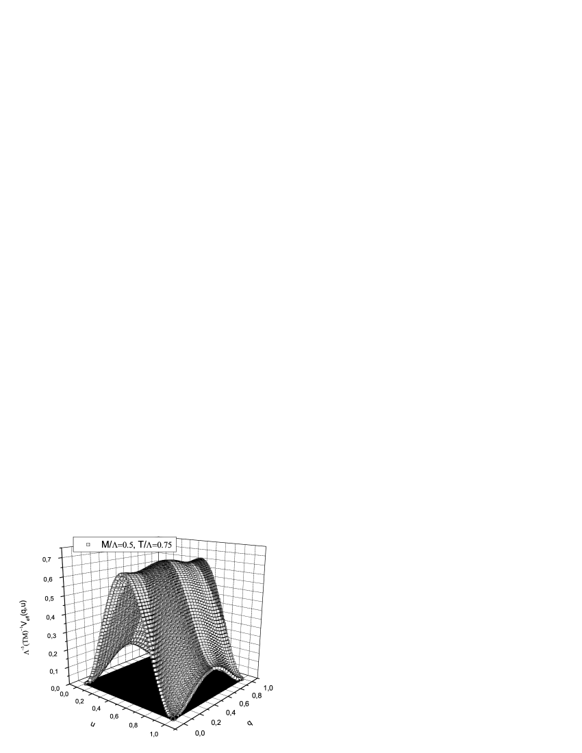
Figure 2: $\Lambda^{-3}(TM)^{-1}V_{eff}(q,u)$ as a function of $q$ and $u$ for $M/\Lambda=0.5$ and $T/\Lambda=0.75$.

An interesting feature of the effective potential is that it is periodic in the dimensionless fields $q$ and $u$ with corresponding periods equal to one. For this reason we have plotted the $V_{eff}(q,u)$ only in the region $[0,1]\times[0,1]$. Note that this periodicity of the effective potential is a consequence of the $Z_{T}(2)\times Z_{M}(2)$ symmetry of the gauge field theory.

We could not find an analytical expression for the effective potential. However the effective potential $M^{-d}V^{M}_{eff}(q)$ (or $T^{-d}V^{T}_{eff}(u)$) can be approximated very well by a function of the form $c\;q^{a}(1-q)^{a}$ where the parameters $c$ and $a$ are determined by a nonlinear fit procedure . In Table 1 we present some values of $c$ and $a$ for several $\rho$ for $d=5$. We see that as $\rho$ increases the parameter $c$ increases linearly with $\rho$ and the parameter $a$ tends to a constant value equal to $2$.

Now for the special case of $\rho=0$ we have:

$$M^{-5}V^{M}_{eff}(q)=\frac{9}{\pi^{2}}\sum_{r=1}^{+\infty}\frac{\sin^{2}(\pi rq)}{r^{5}}=18.87\;q^{2.183}(1-q)^{2.183}$$ (28)

For the case of $\rho\rightarrow+\infty$ we have shown, performing accurate numerical computations, that:

$$\frac{1}{r^{5}}+\sum_{l=1}^{+\infty}\frac{2}{(r^{2}+l^{2}/\rho^{2})^{5/2}}\sim\frac{4}{3}\rho\frac{1}{r^{4}}$$ (29)

Thus from Eqs. (29) and (25)

$$M^{-5}V^{M}_{eff}(q)\sim\frac{12}{\pi^{2}}\rho\sum_{r=1}^{+\infty}\frac{\sin^{2}(\pi rq)}{r^{4}}\sim 2\pi^{2}\rho\;q^{2}(1-q)^{2}$$ (30)

where we have used $x^{2}(1-x)^{2}=\frac{6}{\pi^{4}}\sum_{r=1}^{+\infty}\frac{\sin^{2}(\pi rx)}{r^{4}}$ (for this formula see for example Ref. [10]).

$\rho$	c	c/$\rho$	$a$
0	18.87	-	2.183
0.5	17.78	35.57	2.110
1	21.11	21.11	2.015
2	39.49	19.74	2.000
3	59.22	19.74	2.000
4	78.96	19.74	2.000

Table 1: A very good approximation for the effective potential $M^{-5}V^{M}_{eff}(q)$ is given by a curve of the form $c\;q^{a}(1-q)^{a}$. The parameters $c$ and $a$ are determined with a nonlinear fit procedure for several values of $\rho$ and are presented in the above table. We see that the parameter $c$ is proportional to $\rho$ for $\rho>>1$. The relative errors for the parameters $a$ and $c$ are of the order of a thousandth or smaller and are not presented in this table.

According to Fig. 1 we expect a restoration of $Z_{M}(2)$ symmetry above a temperature $T_{c}$ ($T_{c}>M$) where the system passes from region (A) to region (B). However the perturbative results can not explain the restoration of the $Z_{M}(2)$ symmetry for large temperatures, as the barrier that separates the vacua $q=0$ and $q=1$ increases linearly with the temperature (this is also emphasized in Ref. [4]).

4 A 3-dimensional model with two scalar fields.

In this section we will present an analysis, from our point of view, for the $Z_{M}(2)$ symmetry restoration and more generally for the phase diagram of Fig. 1, taking into account the result for the effective potential of Eq. (24).

We consider that the fields $u=g_{5}B^{3}_{\tau}/2\pi T$ and $q=g_{5}B^{3}_{y}/2\pi M$, are not constant, as it was assumed, but they are dependant on the spatial coordinates $x=(x_{1},x_{2},x_{3})$. Now we can construct a new action by adding to the one loop effective potential the kinetic terms which are obtained by substituting Eqs. (10) and (11) in the original action of the five dimensional gauge theory. Then we have:

$$S_{eff}[q,u]=\frac{2\pi^{2}}{g_{5}^{2}\rho}\int d^{3}x\;(\partial q)^{2}+\frac{2\pi^{2}\rho}{g_{5}^{2}}\int d^{3}x\;(\partial u)^{2}+\frac{1}{TM}\int d^{3}x\;V_{eff}(q,u)$$ (31)

This simple model is viewed as a quantum field theory and the expectation value of an observable quantity $\hat{O}(q,u)$ (an example of an observable quantity is the Polyakov loop in Eq. (38) below) is obtained by the path integral

$$\langle\hat{O}(q,u)\rangle=\frac{\int{\cal D}q{\cal D}u\;\hat{O}(q,u)\;e^{-S_{eff}(q,u)}}{\int{\cal D}q{\cal D}u\;e^{-S_{eff}(q,u)}}$$ (32)

Note that this model is nonrenormalizable as the potential is periodic and thus includes powers of $q$ and $u$ larger than $six$ . However, in this paper, our model is viewed as a low energy effective theory that is valid up to a finite momentum cut-off $\Lambda$. In this way all observable quantities are rendered finite. The momentum cut-off $\Lambda$ could be identified with the momentum cut-off of the original gauge theory.

Our purpose, for the introduction of this scalar model, is to incorporate fluctuations for the scalar fields $q$ and $u$. An estimation of the intensity of fluctuations is given by the inverse of the coefficients in the kinetic terms of Eq.(31). The fluctuations for the field $u$ are controlled by the parameter $g^{2}_{5}/\rho$ and for the field $q$ by $g^{2}_{5}\rho$ where $\rho=T/M$. So, for example, when we increase the temperature $T$ keeping the mass scale $M$ fixed we increase the fluctuations for $q$ and suppress the fluctuations for $u$.

Note that the model possesses four topologically nonequivalent vacua: $(q=0,u=0)$, $(q=0,u=1)$, $(q=1,u=0)$, $(q=1,u=1)$. These vacua are separated by potential barriers, as we see in Fig. 2. According to the above model, the system can jump from one vacuum to another only due to fluctuations of the dimensionless scalar fields $q$ and $u$.

When our system is in region (A) (see Fig. 1) $q$ and $u$ are frozen to one of the four vacua of the model. As the temperature T increases, and the mass scale M is kept fixed, the barrier between the vacua $(q=0,u=0)$ and $(q=0,u=1)$ (or $(q=1,u=0)$ and $(q=1,u=1)$ ) increases rapidly (like $T^{5}$ as we obtain from Eq. (26)). In addition the fluctuations for the field $u$ are getting weaker, thus they can not help the system to jump from one vacuum to another and the field $u$ remains frozen to $u=0$ or to $u=1$.

On the other hand, the barrier between the vacua $(q=0,u=0)$ and $(q=1,u=0)$ (or equivalently between $(q=0,u=1)$ and $(q=1,u=1)$), as we see from Tab. 1, is proportional to $\rho=T/M$. In this case, as it is remarked in the last paragraph, the fluctuations of the field $q$ are getting stronger as the temperature increases, and this can help the system to jump from one vacuum to another and may have as a result the restoration of the $Z_{M}(2)$ symmetry (then the system passes from region (A) to region (B) in Fig. 1).

5 The lattice model

Our aim is to perform numerical computation and to see if the model can confirm the basic features of the phase diagram of Fig. 1. The only way to use this model for numerical computations is to discretise the action of Eq. (31) in the lattice.

We will denote the lattice points by $n=(n_{1},n_{2},n_{3})$ where $n_{1},n_{2},n_{3}$ are integers. If the lattice spacing will be denoted by $a$, then the corresponding physical points are $x_{n}=(an_{1},an_{2},an_{3})$. We remind readers that in this model we assume fixed lattice spacing which is set equal to the inverse value of the momentum cut-off $\Lambda$ of the five dimensional gauge theory.

The lattice action reads:

$$S_{eff}[q,u]= \beta_{g} \frac{\pi^{2}}{2}\sum_{n}\sum_{\mu=1}^{3}\left(\frac{1}{\rho}(q(x_{n}+ae_{\mu})-q(x_{n}))^{2}+\rho\;(u(x_{n}+ae_{\mu})-u(x_{n}))^{2}\right)$$ (33)

$$+ \sum_{n}\;\hat{V}_{eff}(q(x_{n}),u(x_{n}))$$

where $\beta_{g}=4a/g_{5}^{2}$, $e_{\mu}$ are the unit vectors, and we choose to measure all the quantities in the action in units of the lattice spacing.

The potential $\hat{V}_{eff}(q,u)$ is defined as $\hat{V}_{eff}(q,u)=\frac{a^{3}}{TM}V_{eff}(q,u)$. According to this definition we have:

$$\hat{V}_{eff}(q,u)=\hat{V}^{M}_{eff}(q)+\hat{V}^{T}_{eff}(u)+\hat{V}_{eff}^{int}(q,u)$$ (34)

where

$$\hat{V}^{M}_{eff}(q)=4(d-2)m^{d-2}\rho\frac{\Gamma(d/2)}{\pi^{d/2}}\sum_{r=1}^{+\infty}\sin^{2}(\pi rq)[\frac{1}{r^{d}}+\sum_{l=1}^{+\infty}\frac{2}{(r^{2}+l^{2}/\rho^{2})^{d/2}}]$$ (35)

$$\hat{V}^{T}_{eff}(u)=4(d-2)t^{d-2}(1/\rho)\frac{\Gamma(d/2)}{\pi^{d/2}}\sum_{l=1}^{+\infty}\sin^{2}(\pi lu)[\frac{1}{l^{d}}+\sum_{r=1}^{+\infty}\frac{2}{(l^{2}+r^{2}\rho^{2})^{d/2}}]$$ (36)

$$\hat{V}_{eff}^{int}(q,u)=-16(d-2)m^{d-2}\rho\frac{\Gamma(d/2)}{\pi^{d/2}}\sum_{l=1}^{+\infty}\sum_{r=1}^{+\infty}\frac{\sin^{2}(\pi lu)\sin^{2}(\pi rq)}{(r^{2}+l^{2}/\rho^{2})^{d/2}}$$ (37)

Note that we have set $t=Ta$ and $m=Ma$.

The order parameters, according to which the symmetries $Z_{T}(2)$ and $Z_{M}(2)$ are violated or not, are defined by the average values of the Polyakov loops (see Eqs. (7) and (8)) which, for the lattice model we examine, are given by the equations:

$$P_{\tau}(x)=\cos(\pi u(x)),\quad P_{y}(x)=\cos(\pi q(x))$$ (38)

The volume averages of the Polyakov loop are:

$$\bar{P}_{\tau}=\frac{1}{V_{L}}\sum_{\{n\}}P_{\tau}(x_{n}),\quad\bar{P}_{y}=\frac{1}{V_{L}}\sum_{\{n\}}P_{y}(x_{n})$$ (39)

and $V_{L}=V/\alpha^{3}$ is the lattice volume.

So with the lattice simulation we will measure the quantities:

$$|P_{\tau}|=\langle|\bar{P}_{\tau}|\rangle,\quad|P_{y}|=\langle|\bar{P}_{y}|\rangle$$ (40)

The critical values of $t$ (or critical values of $m$) are specified as the values which maximize the susceptibilities:

$$\chi(P_{\tau})=V_{L}\left[\langle(\bar{P}_{\tau})^{2}\rangle-(\langle|\bar{P}_{\tau}|\rangle)^{2}\right],\quad\chi(P_{y})=V_{L}\left[\langle(\bar{P}_{y})^{2}\rangle-(\langle|\bar{P}_{y}|\rangle)^{2}\right]$$ (41)

6 Numerical results

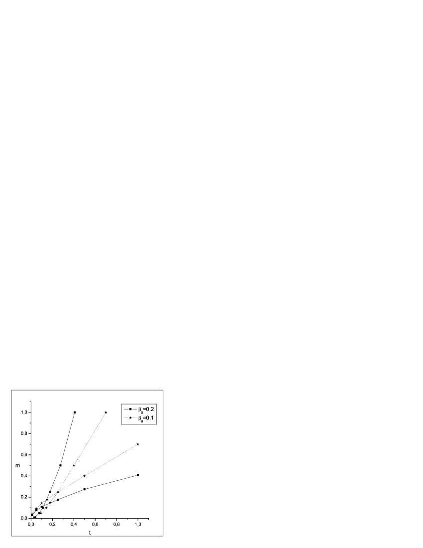
Figure 3: The phase diagram of the model for fixed $\beta_{g}=0.2$ or $0.1$, for finite lattice volume $V_{L}=16^{3}.$

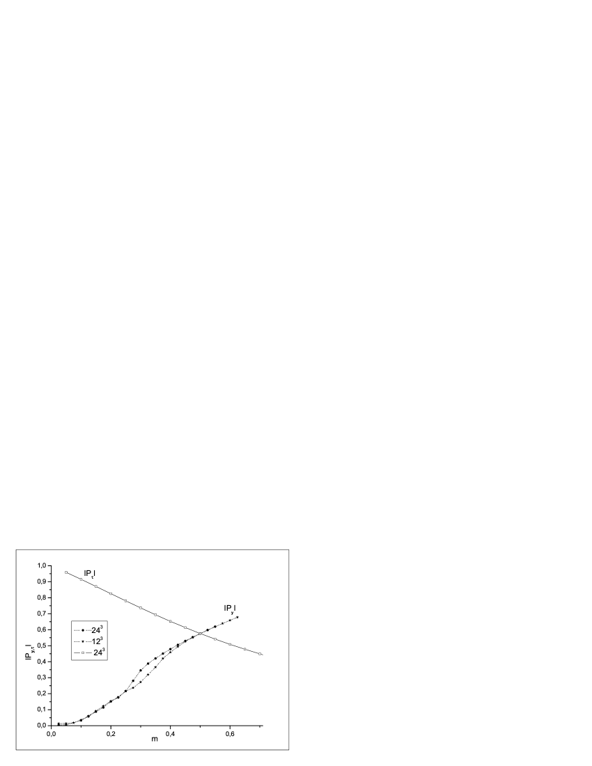
Figure 4: $|P_{y}|$ and $|P_{\tau}|$ as a function of $m$ for $\beta_{g}=0.2$, $t=0.5$ and $V_{L}=12^{3},24^{3}$. We see that as the lattice volume increases the phase transition, which corresponds to $|P_{y}|$ , is getting more sharp. The phase transition for $|P_{\tau}|$ is not shown in this plot.

Figure 5: $\chi(P_{y})$ as a function of $m$ for $\beta_{g}=0.2$, $t=0.5$ and $V_{L}=16^{3},20^{3}$ and $24^{4}$. As the lattice volume increases $m_{c}$ is moving slowly towards the left and, for large lattice volume $V_{L}$, it seems to tend to an asymptotic value.

Figure 6: $Ln(\chi(P_{y})_{max})$ as a function of $Ln(V_{L})$. The discrete points corresponds to $V_{L}=10^{3}$, $12^{3}$, $16^{3}$, $20^{3}$ and $24^{3}$. The continue line corresponds to a best fit curve of the form $Ln(\chi_{max})=a+b\cdot Ln(V_{L})$ for the three bigger volumes.

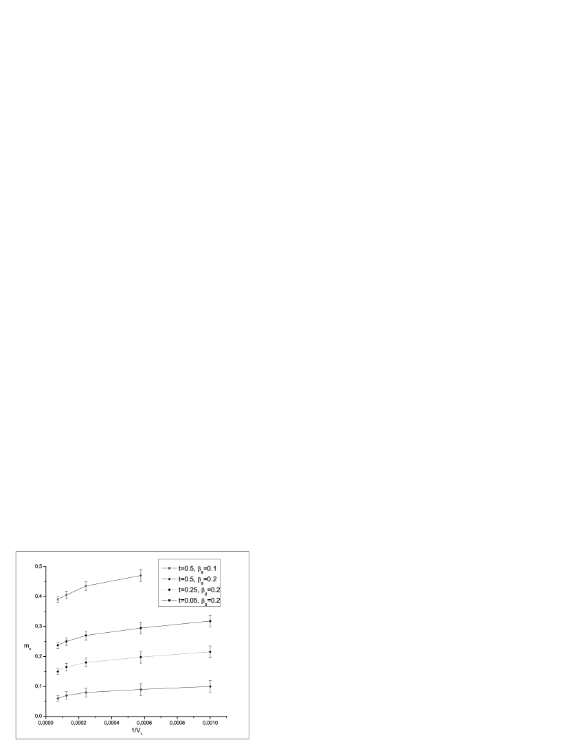
Figure 7: $m_{c}$ for fixed $\beta_{g}=0.2$, $t=0.5,0.25,0.05$ and $\beta_{g}=0.1$, $t=0.5$ for five distinct values of lattice volume $10^{3}$, $12^{3}$, $16^{3}$, $20^{3}$ and $24^{3}$. The lines are there to guide the eye.

In this section we will study numerically the phase diagram $t-m$, for fixed $\beta_{g}$. For this we have performed lattice simulation for several lattice volumes $V_{L}=10^{3},12^{3},16^{3},20^{3}$ and $24^{3}$. Near the peaks of the susceptibilities, for $V_{L}=24^{3}$, where the phase transition happens, we have used samples of 250K measurements which are separated by nine Metropolis iterations. The first 20K measurements were ignored for thermalization. For the other lattice volumes we have used samples with fewer measurements.

In Fig. 3 we have plotted the phase diagram for $\beta_{g}=0.2$ and $0.1$ for finite lattice volume $V_{L}=16^{3}$. We see that it exhibits the main features of Fig. 1, namely it separates the $t-m$ plane into the four distinct regions that correspond to the four phases (A),(B),(C) and (D) of the theory.

The order parameter $|P_{y}|$ as a function of $m$, for $\beta_{g}=0.2$ and $t=0.5$ is shown in Fig. 4. We observe that the phase transition of the system remains continuous even for large volumes $V_{L}=24^{3}$. Note that we have performed computations for several other characteristic values of $t$ and $\beta_{g}$ and the continuous behavior of the order parameter as a function of $m$ is the same.

The corresponding susceptibilities are shown in Fig. 5. The location of the points of the phase transition and the estimation of the relative errors have been done by computing the susceptibility several times in the range where the peak is expected. However we have not used a histogram method as it is not applicable to the model we examine.

From the behavior of the peaks of the susceptibilities it seems that we have a second order phase transition. According to the theory of finite size scaling (see for example Ref. [8]) we expect that the peak depends on the lattice volume as $\chi(P_{y})_{max}=cV_{L}^{b}$ for large values of $V_{L}$, where $b=\gamma/3\nu$ (for the definition of the critical exponents $\gamma$ and $\nu$ see Ref. [8]). This behavior was confirmed numerically, for the model we examine, and it is shown in Fig. 6. The errors in the figure were estimated by the Jackknife method. The critical exponent $b$ was determined by a linear fit and it was found to be, for $\beta_{g}=0.2$ , $b=0.70\pm 0.04$ for $t=0.5$, $b=0.68\pm 0.04$ for $t=0.25$ and $b=0.64\pm 0.04$ for $t=0.05$ using the three bigger volumes. For $\beta_{g}=0.1$ and $t=0.5$ we found that $b=0.66\pm 0.04$. These numerical values for $b$ ($0<b<1$) indicate that we do not have a first order phase transition and possibly the phase transition is of second order. Moreover, this is a strong indication that these phase transitions belong to the same universality class, as the numerical values of these critical exponents are very close and lie in the range of errors. Finally, we note, that these values for $b$ could be equal to the corresponding critical exponent of the 3d ising model $b=0.657$. This numerical value for the critical exponent $b$ was obtained in Ref. [11].

We argue also that the qualitative features of the phase diagram, of Fig. 3, can not be just finite size effects. For this we have plotted in Fig. 7 the critical value $m_{c}$ for several values of $t=0.05,0.25$ and $0.5$, for $\beta_{g}=0.2$ and $0.1$, as a function of lattice volume $V_{L}$. We see that there are small displacements for $m_{c}$ but the arrangement of the critical values does not change as the the lattice volume increases. This indicates that, in the infinite lattice volume limit, the qualitative features of the phase diagram are preserved.

Note that we have not used the data points in Fig. 7 in order to to determine the critical exponent, as a fitting of the form $m_{c}=m_{\infty}+c^{\prime}/V_{L}^{1/3\nu}$ will give unreliable results. The reason is that we have to determine three independent parameters whose values are very sensitive and we have not enough data points with a satisfactory accuracy.

7 Conclusions

We have computed the one loop effective potential for a 5D SU(2) gauge field theory at finite temperature and radius in the case of a background field with two constant components $A^{3}_{y}$ and $A^{3}_{\tau}$.

However the effective potential, which is a perturbative result, can not explain straightforwardly all the qualitative features of the phase diagram of Fig. 1. For this we constructed a phenomenological model by adding to the one loop effective potential kinetic terms (see Eq. (31)). We performed Monte Carlo simulations with the lattice version of this model (see Eq. (33)) and we found a phase diagram, for fixed lattice spacing and $\beta_{g}$, which exhibits all the qualitative features of Fig. 1.

Now the restoration of $Z_{M}(2)$ for large temperatures (or the passing from region (A) to region (B) in Fig. 1) can be understood in the following simplistic way: even though the barrier that separates the vacua of the dimensionless field $q$ increases linearly with the temperature $T$, the fluctuations of $q$ are getting stronger (see section 4), and as it is confirmed by the lattice model, it succeeds in restoring the $Z_{M}(2)$ symmetry. At the same time the fluctuations of $u$ are getting more and more restricted so the field $u$ is frozen to one of its vacuum states.

Finally we remark that the numerical results indicate second order phase transitions, which is an interesting feature of the lattice model of Eq. (33). However, questions like the continuous limit (or nonperturbative renormalizability) are beyond the scope of this paper.

8 Acknowledgements

We would like to thank P. Dimopoulos and K. Anagnostopoulos for reading and comments on the manuscript. We also thank G. Tiktopoulos for valuable discussions, and C. P. Korthals Altes for reading the manuscript and his comments on the constraint effective potential. The work of P.P. was supported by the ”Pythagoras” project of the Greek Ministry of Education. The numerical computations have been carried on the cluster of the Physics Department of NTUA.

9 Appendix: The constraint effective potential for two scalar fields

Generalizing the definition of the constraint effective potential $\widetilde{V}_{eff}$ in Ref. [10] for the case of two order parameters we have:

$$e^{-V\beta R\widetilde{V}_{eff}(t_{4},t_{5})}=\frac{1}{Z}\int{\cal D}A_{\mu}^{\alpha}\delta(t_{4}-\bar{t}_{4})\delta(t_{5}-\bar{t}_{5})e^{-S[A_{\mu}^{\alpha}]}$$ (42)

where

$$\bar{t}_{4}(A_{4}^{\alpha})=\frac{1}{2VR}\int_{0}^{R}dy\int d^{3}x\;TrPe^{ig_{5}\int_{0}^{\beta}A_{4}(x,\tau,y)d\tau}$$ (43)

and

$$\bar{t}_{5}(A_{5}^{\alpha})=\frac{1}{2V\beta}\int_{0}^{\beta}d\tau\int d^{3}x\;TrPe^{ig_{5}\int_{0}^{R}A_{5}(x,\tau,y)dy}$$ (44)

If we use the following representations for the delta functions

$$\delta(t_{4}-\bar{t}_{4})=\int_{-\infty}^{+\infty}d\lambda_{4}e^{i\lambda_{4}(t_{4}-\bar{t}_{4})}$$ (45)

and

$$\delta(t_{5}-\bar{t}_{5})=\int_{-\infty}^{+\infty}d\lambda_{5}e^{i\lambda_{5}(t_{5}-\bar{t}_{5})}$$ (46)

we obtain

$$e^{-V\beta R\widetilde{V}_{eff}(t_{4},t_{5})}=\frac{1}{Z}\int d\lambda_{4}\int\lambda_{5}\int{\cal D}A_{\mu}^{\alpha}\;e^{-S[A_{\mu}^{\alpha}]+i\lambda_{4}(t_{4}-\bar{t}_{4})+i\lambda_{5}(t_{5}-\bar{t}_{5})}$$ (47)

In order to compute the above path integral we use the saddle point method. We split the fields into classical and quantum parts

$$A_{\mu}^{\alpha}=B_{\mu}^{\alpha}+Q_{\mu}^{\alpha}$$ (48)

and

$$\lambda_{4,5}=b_{4,5}+q_{4,5}$$ (49)

We expand the exponent in Eq. (47) up to quadratic terms in quantum fields. The linear terms which are proportional to the equations of motion, according to the saddle point method are required to vanish (for details see Ref. [10] ).

$$\left(-\frac{\delta S}{\delta A_{4,5}^{\alpha}}+ib_{4,5}\frac{\delta\bar{t}_{4,5}}{\delta A_{4,5}^{\alpha}}\right)_{B_{4,5}^{\alpha}}=0$$ (50)

$$-\left(\frac{\delta S}{\delta A_{1,2,3}^{\alpha}}\right)_{B_{\mu}^{\alpha}}=0$$ (51)

$$t_{4,5}-\bar{t}_{4,5}(B_{4,5}^{\alpha})=0$$ (52)

We assume that the background fields $B_{4,5}^{\alpha}$ are constant and have different directions in the isospin space (note that we have also assumed that $B_{1,2,3}^{\alpha}=0$ ). Of course there is not a gauge transformation that can put the two gauge field components in the same direction. However we can perform two rotations in the isospin space. With the first we can put $B_{4}$ towards the generator $T_{3}$ and with the second we can put $B_{5}$ on the plane defined by the generators $T_{3}$ and $T_{1}$. Thus we can write

$$B_{4}=B_{4}^{3}T_{3}$$ (53)

and

$$B_{5}=B_{5}^{3}T_{3}+B_{5}^{1}T_{1}$$ (54)

We will look for a saddle point solution assuming that it is possible to have $b_{4,5}=0$. From Eqs. (50) and (51) we see that the classical field should satisfy the equations of motion for the gauge fields:

$$-\left(\frac{\delta S}{\delta A_{\mu}^{\alpha}}\right)_{B^{\alpha}_{\mu}}=\left(\partial_{\nu}F_{\mu\nu}^{\alpha}+g_{5}\epsilon^{\alpha cb}F_{\mu\nu}^{b}A_{\nu}^{c}\right)_{B^{\alpha}_{\mu}}=0$$ (55)

or

$$\epsilon^{\alpha cb}F_{\mu\nu}^{b}B_{\nu}^{c}=0$$ (56)

Taking into account Eqs. (53) and (54) the only nonzero component of the field tensor is

$$F_{45}^{2}=g_{5}B_{4}^{3}B_{5}^{1}$$ (57)

From Eqs. (56) and (57), for $\mu=5$ and $\alpha=1$, we have

$$(B_{4}^{3})^{2}B_{5}^{1}=0$$ (58)

and, for $\mu=4$ and $\alpha=3,1$, we have

$$(B_{5}^{1})^{2}B_{4}^{3}=0,\>\alpha=3$$ (59)

and

$$B_{4}^{3}B_{5}^{1}B_{5}^{3}=0,\>\alpha=1$$ (60)

These three equations are satisfied only if $B_{4}^{3}=0$ or $B_{5}^{1}=0$. However in general $B_{4}^{3}\neq 0$ (If we assume that $B_{4}^{3}=0$ then we have only one gauge field component and the case is trivial). So we must have $B_{5}^{1}=0$ and thus the two gauge field components $B_{4}$ and $B_{5}$ have the same direction in the group space.

Thus the saddle point we obtain has the form

$$B_{4}=B_{4}^{3}T_{3},\>B_{5}=B_{5}^{3}T_{3},\>b_{4,5}=0$$ (61)

Now if we compute the path integral of Eq. (47), around this saddle point, to one loop order, according to Ref. [10], we see that the result for the constraint effective potential is in agreement with that of Eq. (24) for the one loop effective potential.

References

[1] G. ’t Hooft, Nucl. Phys. B 138 (1978) 1.
[2]Effective potential for the order parameter of gauge theories at finite
temperature, N. Weiss, Phys. Rev. D. 24 (1981); Wilson
line in finite temperature gauge theories, N. Weiss, Phys. Rev.
D. 25 (1981).
[3]Interface tension
in an SU(N) Gauge theory at high temperature, T. Bhattacharya, A.
Gocksch, C. P. Korthals Altes and R. D. Pisarsky, Phys. Rev. Lett.
66 (1991) 988; Z(N) interface tension in a hot SU(N) gauge
theory, T. Bhattacharya, A. Gocksch, C. Korthals Altes and R. D.
Pisarsky, Nucl. Phys. B383 (1992) 497.
[4]A remark on higher dimension induced domain wall defects in our
world, C. P. Korthals Altes and M. Laine, Phys. Lett B511:269
(2001), [hep-ph/0104031].
[5]Finite temperature Z(N) phase transition with Kaluza-Klein gauge
fields, K. Farakos, P. de Forcrand, C. P. Korthals Altes, M. Laine
and M. Vettorazzo, Nucl. Phys. B655:170 (2003), [hep-ph/0207343].
[6]Grand Unification at Intermediate Mass Scales through Extra
Dimensions, K. R. Dienes, E. Dudas and T. Gherghetta, Nucl. Phys.
B 537 (1999) 47, [hep-ph/9806292].
[7]Quantum Field Theory, M. Kaku, Oxford
University Press (1993).
[8]Monte Carlo Methods in Statistical
Physics, M. E. J. Newman and G. T. Barkema, Oxford University
Press (1999).
[9]Cosmological constraints from extra-dimension induced
domainwalls, C. P. Korthals Altes, [hep-ph/0307368].
[10]Constraint effective potential in hot QCD, C. P. Korthals
Altes, Nucl. Phys. B420 (1994) 637-668.
[11]An Introduction to Quantum field
Theory, M. E. Peskin and D. V. Schroeder, Addison-Wesley
Puplishing Company (1995).