CERN-PH-TH/2004-107

hep-ph/0406156

The transverse momentum distribution
of the Higgs boson at the LHC

Massimiliano Grazzini

Theory Division, CERN, CH-1211 Geneva 23, Switzerland

Abstract

We present perturbative predictions for the transverse momentum ($q_{T}$) distribution of the Higgs boson at the LHC. At small $q_{T}$ the logarithmically-enhanced terms are resummed to all orders up to next-to-next-to-leading logarithmic accuracy. The resummed component is consistently matched to the next-to-leading order calculation valid at large $q_{T}$. The results, which implement the most advanced perturbative information that is available at present for this observable, show a good stability with respect to perturbative QCD uncertainties.

hep-ph/0406156

June 2004

The search for the Higgs boson is among the major issues in the LHC physics program [1]. In recent years much effort has been devoted to refining the theoretical predictions for the various Higgs production channels and the corresponding backgrounds, which are now known to next-to-leading order accuracy (NLO) in most of the cases [2]. For the main Standard Model (SM) Higgs production channel, gluon–gluon fusion, even next-to-next-to leading (NNLO) QCD corrections to the total rate have been computed [3]. Nonetheless, predictions for less inclusive observables are definitely required to perform realistic studies. In particular, an accurate knowledge of the transverse-momentum distribution of the Higgs boson can be important to enhance the statistical significance of the signal over the background.

In this contribution we focus on the dominant SM Higgs production channel, gluon–gluon fusion. When the transverse momentum $q_{T}$ of the Higgs boson is of the order of its mass $M_{H}$, the perturbative series is controlled by a small expansion parameter, $\alpha_{\mathrm{S}}(M_{H}^{2})$, and the fixed order prediction is reliable. The leading order (LO) calculation [4] shows that the large-$M_{t}$ approximation ($M_{t}$ being the mass of the top quark) works well as long as both $M_{H}$ and $q_{T}$ are smaller than $M_{t}$. In the framework of this approximation, the NLO QCD corrections have been computed [5, 6, 7].

The small-$q_{T}$ region ($q_{T}\ll M_{H}$) is the most important, because it is here that the bulk of events is expected. In this region the convergence of the fixed-order expansion is spoiled, since the coefficients of the perturbative series in $\alpha_{\mathrm{S}}(M_{H}^{2})$ are enhanced by powers of large logarithmic terms, $\ln^{m}(M_{H}^{2}/q_{T}^{2})$. To obtain reliable perturbative predictions, these terms have to be systematically resummed to all orders in $\alpha_{\mathrm{S}}$ [8] (see also the list of references in Sect. 5 of Ref. [9]). To correctly enforce transverse-momentum conservation, the resummation has to be carried out in $b$ space, where the impact parameter $b$ is the variable conjugate to $q_{T}$ through a Fourier transformation. In the case of the Higgs boson, the resummation has been explicitly worked out at leading logarithmic (LL), next-to-leading logarithmic (NLL) [10], [11] and next-to-next-to-leading logarithmic (NNLL) [12] level. The fixed-order and resummed approaches then have to be consistently matched at intermediate values of $q_{T}$, so as to avoid double counting.

In the following we present predictions for the Higgs boson $q_{T}$ distribution at the LHC within the formalism described in Ref. [13]. In particular, we include the best perturbative information that is available at present: NNLL resummation at small $q_{T}$ and NLO calculation at large $q_{T}$. An important feature of our formalism is that a unitarity constraint on the total cross section is automatically enforced, such that the integral of the spectrum reproduces the known results at NLO [14] and NNLO [3]. More details can be found in Ref. [15]. Other phenomenological studies are presented in [16].

We are going to present quantitative results at NLL+LO and NNLL+NLO accuracy. At NLL+LO (NNLL+NLO) accuracy the NLL (NNLL) resummed result is matched to the LO (NLO) perturbative calculation valid at large $q_{T}$. As for the evaluation of the fixed-order results, the Monte Carlo program of Ref. [5] has been used. The numerical results are obtained by choosing $M_{H}=125$ GeV and using the MRST2002 set of parton distributions [17]. At NLL+LO, LO parton densities and 1-loop $\alpha_{\mathrm{S}}$ have been used, whereas at NNLL+NLO we use NLO parton densities and 2-loop $\alpha_{\mathrm{S}}$.

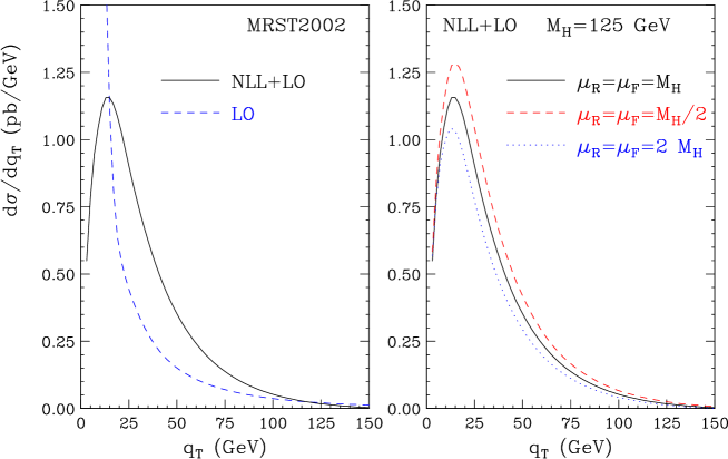
Figure 1: LHC results at NLL+LO accuracy.

The NLL+LO results at the LHC are shown in Fig. 1. In the left panel, the full NLL+LO result (solid line) is compared with the LO one (dashed line) at the default scales $\mu_{F}=\mu_{R}=M_{H}$. We see that the LO calculation diverges to $+\infty$ as $q_{T}\rightarrow 0$. The effect of the resummation starts to be relevant below $q_{T}\sim 100$ GeV. In the right panel we show the NLL+LO band obtained by varying $\mu_{F}=\mu_{R}$ between $1/2M_{H}$ and $2M_{H}$.

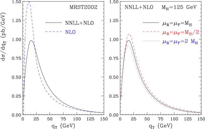
Figure 2: LHC results at NNLL+NLO accuracy.

The corresponding NNLL+NLO results are shown in Fig. 2. In the left panel, the full result (solid line) is compared with the NLO one (dashed line) at the default scales $\mu_{F}=\mu_{R}=M_{H}$. The NLO result diverges to $-\infty$ as $q_{T}\rightarrow 0$ and, at small values of $q_{T}$, it has an unphysical peak that is produced by the numerical compensation of negative leading and positive subleading logarithmic contributions. Notice that at $q_{T}\sim 50$ GeV, the $q_{T}$ distribution sizeably increases when going from LO to NLO and from NLO to NLL+LO. This implies that in the intermediate-$q_{T}$ region there are important contributions that have to be resummed to all orders rather than simply evaluated at the next perturbative order. The resummation effect starts to be visible below $q_{T}\sim 100$ GeV, and it increases the NLO result by about $40\%$ at $q_{T}=50$ GeV. The right panel of Fig. 2 shows the scale dependence computed as in Fig. 1. Comparing Figs. 1 and 2, we see that the NNLL+NLO band is smaller than the NLL+LO one and overlaps with the latter at $q_{T}\raisebox{-1.72218pt}{\hbox to0.0pt{$\,\sim\,$\hss}}\raisebox{1.72218pt}{$\,<\,$}100$ GeV. This suggests a good convergence of the resummed perturbative expansion.

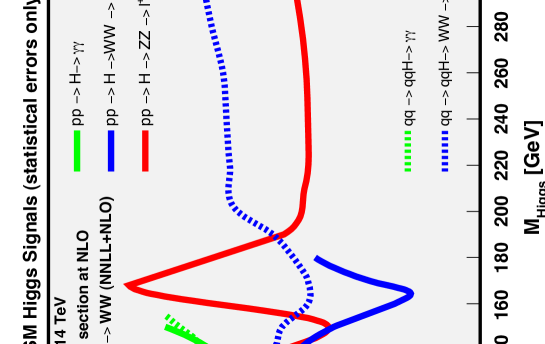
Figure 3: Minimal Higgs discovery luminosities (from M. Dittmar).

A practical application of the results discussed in this contribution has recently been presented [18] in the context of the Higgs search in the channel $pp\rightarrow H\rightarrow WW\rightarrow l\nu l\nu$. In this channel a jet veto is necessary to cut events with high-$q_{T}$ $b$ jets from the $t{\bar{t}}$ background. It is known that the effect of higher order corrections depends on the actual value of this cut [19]. As an approximate way to include higher order effects in the analysis, the QCD-corrected Higgs spectrum presented above has been used in Ref. [18] to reweight signal events generated with the PYTHIA Monte Carlo [20]. The same method has been applied to correct the main $WW$ background, by using a NLL+LO calculation performed within the same resummation formalism [13].

The resulting integrated luminosity needed to discover the Higgs is shown in Fig. 3 and compared with the other channels. We see that, if systematical errors are under control, around the $WW$ threshold the Higgs can be discovered with an integrated luminosity of about half fb^-1.

References

- [1] CMS Coll., Technical Proposal, report CERN/LHCC/94-38 (1994); ATLAS Coll., ATLAS Detector and Physics Performance: Technical Design Report, Vol. 2, report CERN/LHCC/99-15 (1999).
- [2] The Higgs Working Group: Summary Report, to appear in the Proceedings of the Workshop on Physics at TeV Colliders, Les Houches, France, 2003, hep-ph/0406152.
- [3] S. Catani, D. de Florian and M. Grazzini, JHEP 0105 (2001) 025; R. V. Harlander and W. B. Kilgore, Phys. Rev. D 64 (2001) 013015, Phys. Rev. Lett. 88 (2002) 201801; C. Anastasiou and K. Melnikov, Nucl. Phys. B 646 (2002) 220; V. Ravindran, J. Smith, W. L. van Neerven, Nucl. Phys. B 665 (2003) 325.
- [4] R. K. Ellis, I. Hinchliffe, M. Soldate and J. J. van der Bij, Nucl. Phys. B 297 (1988) 221; U. Baur and E. W. Glover, Nucl. Phys. B 339 (1990) 38.
- [5] D. de Florian, M. Grazzini and Z. Kunszt, Phys. Rev. Lett. 82 (1999) 5209.
- [6] V. Ravindran, J. Smith and W. L. Van Neerven, Nucl. Phys. B 634 (2002) 247.
- [7] C. J. Glosser and C. R. Schmidt, JHEP 0212 (2002) 016.
- [8] G. Parisi and R. Petronzio, Nucl. Phys. B 154 (1979) 427; Y. L. Dokshitzer, D. Diakonov and S. I. Troian, Phys. Rep. 58 (1980) 269; J. C. Collins, D. E. Soper and G. Sterman, Nucl. Phys. B 250 (1985) 199.
- [9] S. Catani et al., hep-ph/0005025, in the Proceedings of the CERN Workshop on Standard Model Physics (and more) at the LHC, eds. G. Altarelli and M.L. Mangano (CERN 2000-04, Geneva, 2000), p. 1.
- [10] S. Catani, E. D’Emilio and L. Trentadue, Phys. Lett. B 211 (1988) 335.
- [11] R. P. Kauffman, Phys. Rev. D 45 (1992) 1512.
- [12] D. de Florian and M. Grazzini, Phys. Rev. Lett. 85 (2000) 4678, Nucl. Phys. B 616 (2001) 247.
- [13] S. Catani, D. de Florian and M. Grazzini, Nucl. Phys. B 596 (2001) 299.
- [14] S. Dawson, Nucl. Phys. B 359 (1991) 283; A. Djouadi, M. Spira and P. M. Zerwas, Phys. Lett. B 264 (1991) 440; M. Spira, A. Djouadi, D. Graudenz and P. M. Zerwas, Nucl. Phys. B 453 (1995) 17.
- [15] G. Bozzi, S. Catani, D. de Florian and M. Grazzini, Phys. Lett. B 564 (2003) 65.
- [16] C. Balazs and C. P. Yuan, Phys. Lett. B 478 (2000) 192; E. L. Berger and J. w. Qiu, Phys. Rev. D 67 (2003) 034026; A. Kulesza, G. Sterman, W. Vogelsang, preprint BNL-HET-03/20 [hep-ph/0309264].
- [17] A. D. Martin, R. G. Roberts, W. J. Stirling and R. S. Thorne, Eur. Phys. J. C 28 (2003) 455.
- [18] G. Davatz, G. Dissertori, M. Dittmar, M. Grazzini and F. Pauss, JHEP 0405 (2004) 009.
- [19] S. Catani, D. de Florian and M. Grazzini, JHEP 0201 (2002) 015.
- [20] T. Sjostrand, P. Eden, C. Friberg, L. Lonnblad, G. Miu, S. Mrenna and E. Norrbin, Comput. Phys. Commun. 135 (2001) 238.