Abstract

Theoretical progress in Higgs boson production and background processes is discussed with particular emphasis on QCD corrections at and beyond next-to-leading order as well as next-to-leading order electroweak corrections. The residual theoretical uncertainties of the investigated processes are estimated in detail. Moreover, recent investigations of the MSSM Higgs sector and other extensions of the SM Higgs sector are presented. The potential of the LHC and a high-energy linear $e^{+}e^{-}$ collider for the measurement of Higgs couplings is analyzed.

Abstract

An optimal choice of proper kinematical variables is one of the main steps in using neural networks (NN) in high energy physics. An application of an improved method to the Higgs boson search at the Tevatron leads to an improvement in the NN efficiency by a factor of 1.5-2 in comparison to previous NN studies.
The $\rm p\bar{p}\rightarrow tbH^{\pm}$ production process with Monte Carlo simulations in HERWIG and PYTHIA is studied at the Tevatron, comparing expected cross sections and basic selection variables.

Abstract

We show how LHC Higgs boson production and decay data can be used to extract gauge and fermion couplings of Higgs bosons. Starting with a general multi-Higgs doublet model, we show how successive theoretical assumptions overcome incomplete input data. We also include specific supersymmetric scenarios as a subset of the analysis.

Abstract

estimated for the H/A $\rightarrow\tau\tau$ and H${}^{\pm}\rightarrow\tau\nu$ decay channels in the associated production processes gg $\rightarrow\rm b\bar{\rm b}\rm H/A$ and gb $\rightarrow$tH^± at large tan$\beta$ in CMS. The value of tan$\beta$ can be determined with better than 35% accuracy when statistical, theoretical, luminosity and mass measurement uncertainties are taken into account.

Abstract

We report on the potential for the discovery of a Standard Model Higgs boson with the vector boson fusion mechanism in the mass range $115<M_{H}<500\,{\rm Ge}\kern-1.0pt{\rm V}$ with the ATLAS experiment at the LHC. Feasibility studies at hadron level followed by a fast detector simulation have been performed for $H\rightarrow W^{(*)}W^{(*)}\rightarrow l^{+}l^{-}/\!\!\!p_{T}$, $H\rightarrow\gamma\gamma$ and $H\rightarrow ZZ\rightarrow l^{+}l^{-}q\overline{q}$. The results obtained show a large discovery potential in the range $115<M_{H}<300\,{\rm Ge}\kern-1.0pt{\rm V}$. Results obtained with multivariate techniques are reported for a number of channels.

Abstract

We investigate the scope of heavy neutral Higgs boson decays into chargino/neutralino pairs yielding four-lepton signatures in the context of the Minimal Supersymmetric Standard Model (MSSM), by exploiting all available modes. A preliminary analysis points to the possibility of detection at intermediate values of $\tan\beta$ and $H^{0}/A^{0}$ masses in the region of 400 GeV and above, provided MSSM parameters associated to the Supersymmetric (SUSY) sector of the model are favourable.

Abstract

This paper describes a study of the Higgs associated production with a gauge boson, W or Z, in the Standard Model framework. The W and Z decay leptonically. Higgs Boson masses from 115 to 150 GeV and backgrounds have been generated with the CompHEP generator, and the fast detector simulation CMSJET is used. Results are presented for an integrated luminosity corresponding to 1 year of LHC running at high luminosity.

Abstract

Prospects for searching for the MSSM Higgs bosons in the intencse coupling regime at the LHC are investigated.

Abstract

The existence of charged Higgs bosons is a central prediction of many extensions of the Higgs sector. Recent results for the discrimination between different models are presented. If the charged Higgs mass is comparable to the top quark mass, previous analyses have to be refined. The results of this special case are discussed. Finally, the discovery reach of heavy charged MSSM Higgs bosons is investigated in the $H^{+}\to t\bar{b}$ channel, tagging three $b$-quarks.

Abstract

We demonstrate that Higgs discovery at the LHC is possible in the context of the NMSSM even for those scenarios such that the only strongly produced Higgs boson is a very SM-like CP-even scalar which decays almost entirely to a pair of relatvely light CP-odd states. In combination with other search channels, we are on the verge of demonstrating that detection of at least one of the NMSSM Higgs bosons is guaranteed at the LHC for accumulated luminosity of $300~{}{\rm fb}^{-1}$.

Abstract

Methods for extracting Higgs boson signals at a 1 TeV center-of-mass energy $e^{+}e^{-}$ linear collider are described. In addition, estimates are given for the accuracy with which branching fractions can be measured for Higgs boson decays to $b\bar{b}$, $WW$, $gg$, and $\gamma\gamma$.

1 Higgs Boson Production in Association with Bottom Quarks

1.1 Introduction

In the Standard Model, the production of a Higgs boson in association with $b$ quarks is suppressed by the small size of the Yukawa coupling, $g_{bbh}=m_{b}/v\sim 0.02$. However, in a supersymmetric theory with a large value of $\tan\beta$, the $b$-quark Yukawa coupling can be strongly enhanced, and Higgs production in association with $b$ quarks becomes the dominant production mechanism.

In a four-flavor-number scheme with no $b$ quarks in the initial state, the lowest order processes are the tree level contributions $gg\rightarrow b{\overline{b}}h$ and $q{\overline{q}}\rightarrow b{\overline{b}}h$, illustrated in Fig. 1. The inclusive cross section for $gg\rightarrow b{\overline{b}}h$ develops potentially large logarithms proportional to $L_{b}\equiv\log(Q^{2}/m_{b}^{2})$ which arise from the splitting of gluons into $b\bar{b}$ pairs. Since $Q\gg m_{b}$, the splitting is intrinsically of ${\cal O}(\alpha_{s}L_{b})$, and because the logarithm is potentially large, the convergence of the perturbative expansion may be poor. The convergence can be improved by summing the collinear logarithms to all orders in perturbation theory through the use of $b$ quark parton distributions (the five-flavor-number scheme) [4] at the factorization scale $\mu_{F}=Q$. This approach is based on the approximation that the outgoing $b$ quarks are at small transverse momentum. Thus the incoming $b$ partons are given zero transverse momentum at leading order, and acquire transverse momentum at higher order. In the five-flavor-number scheme, the counting of perturbation theory involves both $\alpha_{s}$ and $1/L_{b}$. In this scheme, the lowest order inclusive process is $b{\overline{b}}\rightarrow h$, see Fig. 2. The first order corrections contain the ${\cal O}(\alpha_{s})$ corrections to $b{\overline{b}}\rightarrow h$ and the tree level process $gb\rightarrow bh$, see Fig. 3, which is suppressed by ${\cal O}(1/L_{b})$ relative to $b{\overline{b}}\rightarrow h$ [5]. It is the latter process which imparts transverse momentum to the $b$ quarks. The relevant production mechanism depends on the final state being observed. For inclusive Higgs production it is $b{\overline{b}}\rightarrow h$, while if one demands that at least one $b$ quark be observed at high-$p_{T}$, the leading partonic process is $gb\rightarrow bh$. Finally, if two high-$p_{T}$ $b$ quarks are required, the leading subprocess is $gg\rightarrow b{\overline{b}}h$.

The leading order (LO) predictions for these processes have large uncertainties due to the strong dependence on the renormalization/factorization scales and also due to the scheme dependence of the $b$-quark mass in the Higgs $b$-quark Yukawa coupling. The scale and scheme dependences are significantly reduced when higher-order QCD corrections are included.

Section 2 describes the setup for our analysis, and in Section 3 we compare the LO and NLO QCD results for the production of a Higgs boson with two high-$p_{T}$ $b$ jets. Section 4 contains a discussion of the production of a Higgs boson plus one high-$p_{T}$ $b$ jet at NLO, including a comparison of results within the four-flavor-number and the five-flavor-number schemes. We consider the corresponding inclusive Higgs cross sections in Section 5. Although motivated by the MSSM and the possibility for enhanced $b$ quark Higgs boson couplings, all results presented here are for the Standard Model. To a very good approximation the corresponding MSSM results can be obtained by rescaling the bottom Yukawa coupling [6, 7].

Figure 1: Sample Feynman diagrams for $gg\rightarrow b{\overline{b}}h$ and $q{\overline{q}}\rightarrow b{\overline{b}}h$ production.

Figure 2: Feynman diagram for $b{\overline{b}}\rightarrow h$ production.

Figure 3: Feynman diagrams for $gb\rightarrow bh$ production.

1.2 Setup

All results are obtained using the CTEQ6L1 parton distribution functions (PDFs) [8] for lowest order cross sections and CTEQ6M PDFs for NLO results. The top quark is decoupled from the running of $m_{b}(\mu)$ and $\alpha_{s}(\mu)$ and the NLO (LO) cross sections are evaluated using the $2$ ($1$)-loop evolution of $\alpha_{s}(\mu)$ with $\alpha_{s}^{NLO}(M_{Z})=0.118$. We use the ${\overline{\rm MS}}$ running $b$ quark mass, $m_{b}(\mu)$, evaluated at $2$ ($1$)-loop for $\sigma_{NLO}$ ($\sigma_{LO}$), with the $b$ pole mass taken as $m_{b}=4.62$ GeV. The dependence of the rates on the renormalization ($\mu_{R}$) and factorization $(\mu_{F})$ scales is investigated [5, 6, 7, 9, 10] in order to estimate the uncertainty of the predictions for the inclusive Higgs production channel and for the Higgs plus $1~{}b$-jet channel. The dependence of the Higgs plus $2~{}b$- jet rates on the renormalization ($\mu_{R}$) and factorization $(\mu_{F})$ scales has been investigated elsewhere [6, 7] and here we fix $\mu=\mu_{R}=\mu_{F}=(2m_{b}+M_{h})/4$, motivated by the studies in Refs. [1, 2, 3, 5, 6, 7, 9, 10].

In order to reproduce the experimental cuts as closely as possible for the case of Higgs plus 1 or 2 high-$p_{T}$ $b$ quarks, we require the final state $b$ and ${\overline{b}}$ to have a pseudorapidity $\mid\eta\mid<2$ for the Tevatron and $\mid\eta\mid<2.5$ for the LHC. To better simulate the detector response, the gluon and the $b/{\overline{b}}$ quarks are treated as distinct particles only if the separation in the azimuthal angle-pseudorapidity plane is $\Delta R>0.4$. For smaller values of $\Delta R$, the four-momentum vectors of the two particles are combined into an effective $b$/${\overline{b}}$ quark momentum four-vector. All results presented in the four-flavor-number scheme have been obtained independently by two groups with good agreement [6, 7, 11, 12].

1.3 Higgs + 2 $b$ Jet Production

Requiring two high-$p_{T}$ bottom quarks in the final state reduces the signal cross section with respect to that of the zero and one $b$-tag cases, but it also greatly reduces the background. It also ensures that the detected Higgs boson has been radiated off a $b$ or ${\overline{b}}$ quark and the corresponding cross section is therefore unambiguously proportional to the square of the $b$-quark Yukawa coupling at leading order, while at next-to-leading order this property is mildly violated by closed top-quark loops [6, 7]. The parton level processes relevant at lowest order are $gg\rightarrow b{\overline{b}}h$ and $q{\overline{q}}\rightarrow b{\overline{b}}h$, as illustrated in Fig. 1. Searches for the neutral MSSM Higgs bosons $h,H,A$ produced in association with $b$ quarks have been performed at the Tevatron [13].

The rate for Higgs plus 2 high-$p_{T}$ $b$ jets has been computed at NLO QCD in Refs. [6, 7] and is shown in Fig. 4 for both the Tevatron and the LHC. The NLO QCD corrections modify the LO predictions by $\raisebox{-3.69899pt}{~{}\shortstack{$<$ \\ [-0.07cm] $\sim$}}~{}30\%$ at the Tevatron and $\raisebox{-3.69899pt}{~{}\shortstack{$<$ \\ [-0.07cm] $\sim$}}~{}50\%$ at the LHC. The total cross section plots include a cut on $p_{T}^{b/{\overline{b}}}>20$ GeV, which has a significant effect on the cross sections. We show the dependence of the cross section on this cut in Fig. 5. The NLO corrections are negative at large values of the cut on $p^{b/\bar{b}}_{T}$ and tend to be positive at small values of $p^{b/\bar{b}}_{T}$.

Figure 4: Total cross sections for $p{\overline{p}}(pp)\rightarrow b{\overline{b}}h+X$ at the Tevatron and the LHC as a function of the Higgs mass $M_{h}$ with two high-$p_{T}$ $b$ jets identified in the final state. The $b/\bar{b}$ quarks are required to satisfy $p_{T}^{b/\bar{b}}>20~{}GeV$. We fix $\mu=\mu_{R}=\mu_{F}=(2m_{b}+M_{h})/4$.

Figure 5: Total cross sections for $p{\overline{p}}(pp)\rightarrow b{\overline{b}}h+X$ at the Tevatron and the LHC as a function of the cut $p_{T{\rm cut}}$ in $p_{T}^{b/\bar{b}}$ for a Higgs mass $M_{h}=120$ GeV with two high-$p_{T}$ $b$ jets identified in the final state. We fix $\mu=\mu_{R}=\mu_{F}=(2m_{b}+M_{h})/4$.

1.4 Higgs + 1 $b$ Jet Production

The associated production of a Higgs boson plus a single $b$ quark (or $\bar{b}$ quark) is a promising channel for Higgs production in models with enhanced $b{\overline{b}}h$ couplings. The cross section is an order of magnitude larger than that for Higgs plus 2 high-$p_{T}$ $b$ jet production for the cuts imposed in our analysis.

In the four-flavor-number scheme, this process has been computed to NLO, with the momentum of one of the $b$ quarks integrated over [6, 11, 12]. This integration yields a potentially large factor $L_{b}$. Both the total cross sections and the dependence on the $p_{T}^{b,{\overline{b}}}$ cut at the Tevatron and the LHC are shown in Figs. 6 and 7. The NLO corrections increase the cross section by $\raisebox{-3.69899pt}{~{}\shortstack{$<$ \\ [-0.07cm] $\sim$}}~{}50\%$ at the Tevatron and $\raisebox{-3.69899pt}{~{}\shortstack{$<$ \\ [-0.07cm] $\sim$}}~{}80\%$ at the LHC. The renormalization/factorization scales are varied around the central value $\mu=\mu_{R}=\mu_{F}\equiv(2m_{b}+M_{h})/4$. At the Tevatron, the upper bands of the curves for the four-flavor-number scheme in Figs. 6 and 7 correspond to $\mu_{R}=\mu_{F}=2\mu$, while the lower bands correspond to $\mu_{R}=\mu_{F}=\mu/2$. The scale dependence is more interesting at the LHC, where the upper bands are obtained with $\mu_{R}=\mu/2$ and $\mu_{F}=2\mu$, while the lower bands correspond to $\mu_{R}=2\mu$ and $\mu_{F}=\mu/2$. At both the Tevatron and the LHC, the width of the error band below the central value ($\mu=\mu_{R}=\mu_{F}$) is larger than above.

In the five-flavor-number scheme, the NLO result consists of the lowest order process, $bg\rightarrow bh$, along with the ${\cal O}(\alpha_{s})$ and ${\cal O}(1/L_{b})$ corrections, which are of moderate size for our scale choices [9]. The potentially large logarithms $L_{b}$ arising in the four-flavor-number scheme have been summed to all orders in perturbation theory by the use of $b$ quark PDFs. In the five-flavor-number scheme, the upper bands of the curves for the Tevatron in Figs. 6 and 7 correspond to $\mu_{R}=\mu$ and $\mu_{F}=2\mu$, while the lower bands correspond to $\mu_{R}=\mu/2$ and $\mu_{F}=\mu$. At the LHC, the upper bands are obtained with $\mu_{R}=\mu$ and $\mu_{F}=2\mu$, while the lower bands correspond to $\mu_{R}=2\mu$ and $\mu_{F}=\mu/2$. The two approaches agree within their scale uncertainties, but the five-flavor-number scheme tends to yield larger cross sections as can be inferred from Figs. 6 and 7.

Contributions involving closed top-quark loops have not been included in the five-flavor-number scheme calculation of Ref. [9]. This contribution is negligible in the MSSM for large $\tan\beta$. In the four-flavor scheme, the closed top-quark loops have been included and in the Standard Model reduce the total cross section for the production of a Higgs boson plus a single $b$ jet by $\sim-7\%$ at the Tevatron and $\sim-13~{}\%$ at the LHC for $M_{h}=120$ GeV [11, 12].

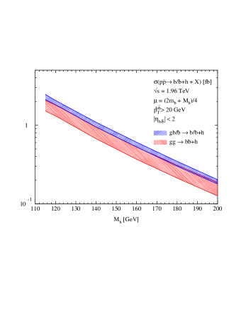
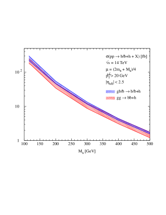
Figure 6: Total cross sections for $p{\overline{p}}(pp)\rightarrow b{\overline{b}}h+X$ at the Tevatron and the LHC as a function of the Higgs mass $M_{h}$ with one high-$p_{T}$ $b$ jet identified in the final state. The $b(\bar{b})$ quark is required to satisfy $p_{T}^{b/\bar{b}}>20~{}\mbox{GeV}$. We vary the renormalization/factorization scales around the central value $\mu=\mu_{R}=\mu_{F}=(2m_{b}+M_{h})/4$ as described in the text.

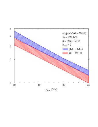
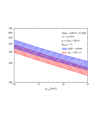
Figure 7: Total cross sections for $p{\overline{p}}(pp)\rightarrow b{\overline{b}}h+X$ at the Tevatron and the LHC as a function of the cut $p_{T{\rm cut}}$ in $p_{T}^{b/\bar{b}}$ for a Higgs mass $M_{h}=120$ GeV with one high-$p_{T}$ $b$ jet identified in the final state. We vary the renormalization/factorization scales around the central value $\mu=\mu_{R}=\mu_{F}=(2m_{b}+M_{h})/4$ as described in the text.

1.5 Inclusive Higgs Boson Production

If the outgoing $b$ quarks are not observed, then the dominant process for Higgs production in the five-flavor-number scheme at large values of $\tan\beta$ is $b{\overline{b}}\rightarrow h$. This final state contains two spectator $b$ quarks (from the gluon splittings) which tend to be at low transverse momentum. At the LHC this state can be identified through the decays into $\mu^{+}\mu^{-}$ and $\tau^{+}\tau^{-}$ for the heavy Higgs bosons $H,A$ at large values of $\tan\beta$ in the MSSM [14]. The $b{\overline{b}}\rightarrow h$ process has been computed to NLO [5] and NNLO [10] in perturbative QCD. The rate depends on the choice of renormalization/factorization scale $\mu_{R/F}$, and at NLO a significant scale dependence remains. The scale dependence becomes insignificant at NNLO. It has been argued that the appropriate factorization scale choice is $\mu_{F}=(M_{h}+2m_{b})/4$ [2, 3] and it is interesting to note that at this scale, the NLO and NNLO results nearly coincide [10].

An alternative calculation is based on the processes $gg\to b\bar{b}h$ and $q\bar{q}\to b\bar{b}h$ (four-flavor-number scheme), which has been calculated at NLO [6, 11, 12]. Despite the presence of the logarithms $L_{b}$ in the calculation based on $gg\to b\bar{b}h$, which are not resummed, it yields a reliable inclusive cross section, as evidenced by Fig. 8. A sizeable uncertainty due to the renormalization and factorization scale dependence remains which might reflect that the logarithms $L_{b}$ are not resummed in this approach, so that the perturbative convergence is worse than in the corresponding case of $t\bar{t}h$ production [15]. In the Standard Model, the closed top-quark loops have been included in the four-flavor-number calculation and reduce the inclusive NLO total cross section for $pp(p{\overline{p}})\rightarrow b{\overline{b}}h$ by $\sim-4\%$ at the Tevatron and $\sim-9\%$ at the LHC for $M_{h}=120$ GeV [11, 12]. In the MSSM, the closed top quark loops are negligible for large $\tan\beta$ [6, 7].

The NLO four-flavor-number scheme calculation is compared with the NNLO calculation of $b\bar{b}\to h$ (five-flavor-number scheme) in Fig. 8. The two calculations agree within their respective scale uncertainties for small Higgs masses, while for large Higgs masses the five-flavor-number scheme tends to yield larger cross sections. Note that closed top-quark loops have not been included in the NNLO calculation of $b\bar{b}\to h$ [10].

To all orders in perturbation theory the four- and five-flavor number schemes are identical, but the way of ordering the perturbative expansion is different and the results do not match exactly at finite order. The quality of the approximations in the two calculational schemes is difficult to quantify, and the residual uncertainty of the predictions may not be fully reflected by the scale variation displayed in Fig. 8.

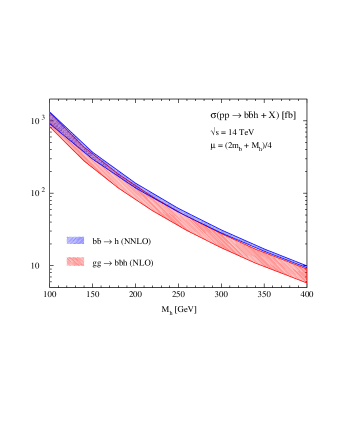
Figure 8: Total cross sections for $p{\overline{p}}(pp)\rightarrow b{\overline{b}}h+X$ at the Tevatron and the LHC as a function of the Higgs mass $M_{h}$ with no $b$ jet identified in the final state. The error bands correspond to varying the scale from $\mu_{R}=\mu_{F}=(2m_{b}+M_{h})/8$ to $\mu_{R}=\mu_{F}=(2m_{b}+M_{h})/2$. The NNLO curves are from Ref. [10].

1.6 Conclusions

We investigated $b\bar{b}h$ production at the Tevatron and the LHC, which is an important discovery channel for Higgs bosons at large values of $\tan\beta$ in the MSSM, where the bottom Yukawa coupling is strongly enhanced [13, 14]. Results for the cross sections with two tagged $b$ jets have been presented at NLO including transverse-momentum and pseudorapidity cuts on the $b$ jets which are close to the experimental requirements. The NLO corrections modify the predictions by up to $50\%$ and reduce the theoretical uncertainties significantly. For the cases of one and no tagged $b$ jet in the final state we compared the results in the four- and five-flavor-number schemes. Due to the smallness of the $b$ quark mass, large logarithms $L_{b}$ might arise from phase space integration in the four-flavor-number scheme, which are resummed in the five-flavor-number scheme by the introduction of evolved $b$ parton densities. The five-flavor-number scheme is based on the approximation that the outgoing $b$ quarks are at small transverse momentum. Thus the incoming $b$ partons are given zero transverse momentum at leading order, and acquire transverse momentum at higher order. The two calculational schemes represent different perturbative expansions of the same physical process, and therefore should agree at sufficiently high order. It is satisfying that the NLO (and NNLO) calculations presented here agree within their uncertainties. This is a major advance over several years ago, when comparisons of $b\bar{b}\to h$ at NLO and $gg\to b\bar{b}h$ at LO were hardly encouraging [1, 16].

2 The total Cross Section $gg\rightarrow H$ at Hadron Colliders

The most important mechanism for Standard Model (SM) Higgs boson production at hadron colliders is gluon–gluon fusion through a heavy (top) quark loop [17]. Next-to-leading order (NLO) QCD corrections to this process were found to be large [18, 19, 20]: their effect increases the leading order (LO) cross section by about 80–100$\%$, thus leading to very uncertain predictions and, possibly, casting doubts on the reliability of the perturbative QCD expansion.

Recent years have witnessed a substantial improvement of this situation. The NLO corrections are well approximated [21] by the large-$M_{t}$ ($M_{t}$ being the mass of the top quark) limit. Using this approximation considerably simplifies the evaluation of higher-order terms, and the calculation of the next-to-next-to-leading order (NNLO) corrections has been completed [22, 23, 24, 25, 26, 27]. Moreover, the logarithmically-enhanced contributions from multiple soft-gluon emission have been consistently included, up to next-to-next-to-leading logarithmic (NNLL) accuracy, in the calculation [28]. An important point is that the origin of the dominant perturbative contributions has been identified and understood: the bulk of the radiative corrections is due to virtual and soft-gluon terms. Having those terms under control allows to reliably predict the value of the cross section and, more importantly, to reduce the associated perturbative (i.e. excluding the uncertainty form parton densities) uncertainty below about $\pm 10\%$ [28], as discussed below.

In this contribution we present QCD predictions for the total cross section, including soft-gluon resummation, and we discuss the present theoretical uncertainties. Denoting the Higgs boson mass by $M_{H}$ and the collider centre–of–mass energy by $\sqrt{s}$, the resummed cross section can be written as [28]

$$\sigma^{\rm(res)}(s,M_{H}^{2})=\sigma^{\rm(SV)}(s,M_{H}^{2})+\sigma^{\rm(match.)}(s,M_{H}^{2})\;\;,$$ (1)

where $\sigma^{\rm(SV)}$ contains the virtual and soft-gluon terms, and $\sigma^{\rm(match.)}$ includes the remaing hard-radiation terms. $\sigma^{\rm(SV)}$, which gives the bulk of the QCD radiative corrections at the Tevatron and the LHC, is obtained through the resummation of the large logarithmic soft-gluon contributions. $\sigma^{\rm(match.)}$ is given by the fixed-order cross section minus the corresponding fixed-order truncation of $\sigma^{\rm(SV)}$. The order of magnitude of the relative contribution from $\sigma^{\rm(match.)}$ is of ${\cal O}(10\%)$ and of ${\cal O}(1\%)$ at NLO and NNLO, respectively. Therefore, $\sigma^{\rm(match.)}$ quantitatively behaves as naively expected from a power series expansion whose expansion parameter is $\alpha_{\mathrm{S}}\sim 0.1$. We expect that the presently unknown (beyond NNLO) corrections to $\sigma^{\rm(match.)}$ have no practical quantitative impact on the QCD predictions for Higgs boson production at the Tevatron and the LHC.

The NNLO and NNLL cross sections at the LHC (Tevatron) are plotted in Fig. 9 (Fig. 10) in the mass range $M_{H}=100$–300 GeV ($M_{H}=100$–200 GeV). The central curves are obtained by fixing the factorization ($\mu_{F}$) and renormalization ($\mu_{R}$) scales at the default value $\mu_{F}=\mu_{R}=M_{H}$. The bands are obtained by varying $\mu_{F}$ and $\mu_{R}$ simultaneously and independently in the range $0.5M_{H}\leq\mu_{F},\mu_{R}\leq 2M_{H}$ with the constraint $0.5\leq\mu_{F}/\mu_{R}\leq 2$. The results in Figs. 9 and 10 are obtained by using the NNLO densities of the MRST2002 [29] set of parton distributions. Another NNLO set (set A02 from here on) of parton densities has been released in Ref. [30]. Tables with detailed numerical values of Higgs boson cross sections (using both MRST2002 and A02 parton densities) can be found in Ref. [28]. The NNLL cros sections are larger than the NNLO ones; the increase is of about $6\%$ at the LHC and varies from about $12\%$ (when $M_{H}=100$ GeV) to about $15\%$ (when $M_{H}=200$ GeV) at the Tevatron.

Figure 9: NNLL and NNLO cross sections at the LHC, using MRST2002 parton densities.

Figure 10: NNLL and NNLO cross sections at the Tevatron ($\sqrt{s}=1.96$ TeV), using MRST2002 parton densities.

We now would like to summarize the various sources of uncertainty that still affect the theoretical prediction of the Higgs production cross section, focusing on the low-$M_{H}$ region ($M_{H}\raisebox{-1.72218pt}{\hbox to0.0pt{$\,\sim\,$\hss}}\raisebox{1.72218pt}{$\,<\,$}200$ GeV). The uncertainty has basically two origins: the one originating from still uncalculated (perturbative) radiative corrections, and the one due to our limited knowledge of the parton distributions.

Uncalculated higher-order QCD contributions are the most important source of uncertainty on the radiative corrections. A method, which is customarily used in perturbative QCD calculations, to estimate their size is to vary the renormalization and factorization scales around the hard scale $M_{H}$. In general, this procedure can only give a lower limit on the ‘true’ uncertainty. In fact, the LO and NLO bands do not overlap [23, 28]. However, the NLO and NNLO bands and, also, the NNLO and NNLL bands do overlap. Furthermore, the central value of the NNLL bands lies inside the corresponding NNLO bands (see Figs. 9 and 10). This gives us confidence in using scale variations to estimate the uncertainty at NNLO and at NNLL order.

Performing scale variations we find the following results. At the LHC, the NNLO scale dependence ranges from about $\pm 10\%$ when $M_{H}=120$ GeV, to about $\pm 9\%$ when $M_{H}=200$ GeV. At NNLL order, it is about $\pm 8\%$ when $M_{H}\raisebox{-1.72218pt}{\hbox to0.0pt{$\,\sim\,$\hss}}\raisebox{1.72218pt}{$\,<\,$}200$ GeV. At the Tevatron, when $M_{H}\raisebox{-1.72218pt}{\hbox to0.0pt{$\,\sim\,$\hss}}\raisebox{1.72218pt}{$\,<\,$}200$ GeV, the NNLO scale dependence is about $\pm 13\%$, whereas the NNLL scale dependence is about $\pm 8\%$.

Another method to estimate the size of higher-order corrections is to compare the results at the highest order that is available with those at the previous order. Considering the differences between the NNLO and NNLL cross sections, we obtain results that are consistent with the uncertainty estimated from scale variations.

To estimate higher-order contributions, we also investigated the impact of collinear terms, which are subdominant with respect to the soft-gluon contributions. Performing the resummation of the leading collinear terms, we found negligible numerical effects [28]. The uncertainty coming from these terms can thus be safely neglected.

A different and relevant source of perturbative QCD uncertainty comes from the use of the large-$M_{t}$ approximation. The comparison [21] between the exact NLO cross section with the one obtained in the large-$M_{t}$ approximation (but rescaled with the full Born result, including its exact dependence on the masses of the top and bottom quarks) shows that the approximation works well also for $M_{H}\raisebox{-1.72218pt}{\hbox to0.0pt{$\,\sim\,$\hss}}\raisebox{1.72218pt}{$\,>\,$}M_{t}$. This is not accidental. In fact, the higher-order contributions to the cross section are dominated by the radiation of soft partons, which is weakly sensitive to mass of the heavy quark in the loop at the Born level. The dominance of soft-gluon effects persists at NNLO [23] and it is thus natural to assume that, having normalized our cross sections with the exact Born result, the uncertainty ensuing from the large-$M_{t}$ approximation should be of order of few per cent for $M_{H}\raisebox{-1.72218pt}{\hbox to0.0pt{$\,\sim\,$\hss}}\raisebox{1.72218pt}{$\,<\,$}200$ GeV, as it is at NLO.

Besides QCD radiative corrections, electroweak corrections have also to be considered. The ${\cal O}(G_{F}M_{t}^{2})$ dominant corrections in the large-$M_{t}$ limit have been computed and found to give a very small effect [31].

The other independent and relevant source of theoretical uncertainty in the cross section is the one coming from parton distributions.

The most updated sets of parton distributions are MRST2002 [29], A02 [30] and CTEQ6 [32]. However, the CTEQ collaboration does not provide a NNLO set, so that a consistent comparison with MRST2002 and A02 can be performed only at NLO. At the LHC, we find that the CTEQ6M results are slightly larger than the MRST2002 ones, the differences decreasing from about $2\%$ at $M_{H}=100$ GeV to below $1\%$ at $M_{H}=200$ GeV. The A02 results are instead slightly smaller than the MSRT2002 ones, the difference being below $3\%$ for $M_{H}\raisebox{-1.72218pt}{\hbox to0.0pt{$\,\sim\,$\hss}}\raisebox{1.72218pt}{$\,<\,$}200$ GeV. At the Tevatron, CTEQ6 (A02) cross sections are smaller than the MRST2002 ones, the differences increasing from $6\%$ ($7\%$) to $10\%$ ($9\%$) when $M_{H}$ increases from $100$ GeV to $200$ GeV. These discrepancies arise because the gluon density (in particular, its behaviour as a function of the momentum fraction $x$) is different in the three sets of parton distributions. The larger discrepancies at the Tevatron are not unexpected, since here the gluon distribution is probed at larger values of $x$, where differences between the three sets are maximal.

All three NLO sets include a study of the effect of the experimental uncertainties in the extraction of the parton densities from fits of hard-scattering data. The ensuing uncertainty on the Higgs cross section at NLO is studied in Ref. [33] (note that Ref. [33] uses the MRST2001 set [34], while we use the MRST2002 set). The cross section differences that we find at NLO are compatible with this experimental uncertainty, which is about $\pm 3$–$5\%$ (depending on the set) at the LHC and about $\pm 5$–$15\%$ (in the range $M_{H}=100$–200 GeV) at the Tevatron.

In summary, the NLO Higgs boson cross section has an uncertainty from parton densities that is smaller than the perturbative uncertainty, which (though difficult to quantify with precision) is of the order of many tens of per cent.

We now consider the NNLL (and NNLO) cross sections. The available NNLO parton densities are from the MRST2002 and A02 sets, but only the A02 set includes an estimate of the corresponding experimental errors. Computing the effect of these errors on the cross section, we find [28] that the A02 results have an uncertainty of about $\pm 1.5\%$ at the LHC and from about $\pm 3\%$ to about $\pm 7\%$ (varying $M_{H}$ from 100 to 200 GeV) at the Tevatron.

Comparing the cross sections obtained by using the A02 and MSRT2002 sets, we find relatively large differences [28] that cannot be accounted for by the errors provided in the A02 set. At the LHC, the A02 results are larger than the MRST2002 results, and the differences go from about $8\%$ at low masses to about $2\%$ at $M_{H}=200$ GeV. At the Tevatron, the A02 results are smaller than the MRST2002 results, with a difference going from about $7\%$ at low $M_{H}$ to about $14\%$ at $M_{H}=200$ GeV.

The differences in the cross sections are basically due to differences in the gluon–gluon luminosity, which are typically larger than the estimated uncertainty of experimental origin. In particular, the differences between the $gg$ luminosities appear to increase with the perturbative order, i.e. going from LO to NLO and to NNLO (see also Figs. 13 and 14 in Ref. [28]). We are not able to trace the origin of these differences. References [30] and [29] use the same (though approximated) NNLO evolution kernels, but the A02 set is obtained through a fit to deep-inelastic scattering (DIS) data only, whereas the MRST2002 set is based on a fit of DIS, Drell–Yan and Tevatron jet data (note that not all these observables are known to NNLO accuracy).

The extraction of the parton distributions is also affected by uncertainties of theoretical origin, besides those of experimental origin. These ‘theoretical’ errors are more difficult to quantify. Some sources of theoretical errors have recently been investigated by the MRST collaboration [35], showing that they can have non neglible effects on the parton densities and, correspondingly, on the Higgs cross section. At the Tevatron these effect can be as large as $5\%$, but they are only about $2\%$ at the LHC.

As mentioned above, the MRST2002 and A02 sets use approximated NNLO evolution kernels [36], which should be sufficiently accurate. This can be checked as soon the exact NNLO kernels are available [37].

We conclude that the theoretical uncertainties of perturbative origin in the calculation of the Higgs production cross section, after inclusion of both NNLO corrections and soft-gluon resummation at the NNLL level, are below 10% in the low-mass range ($M_{H}\raisebox{-1.72218pt}{\hbox to0.0pt{$\,\sim\,$\hss}}\raisebox{1.72218pt}{$\,<\,$}200$ GeV). This amounts to an improvement in the accuracy of almost one order of magnitude with respect to the predictions that were available just few years ago. Nonetheless, there are uncertainties in the (available) parton densities alone that can reach values larger than 10%, and that are not fully understood at present.

3 The $q_{T}$ Spectrum of the Higgs Boson at the LHC

An accurate theoretical prediction of the transverse-momentum ($q_{T}$) distribution of the Higgs boson at the LHC can be important to enhance the statistical significance of the signal over the background. In fact, a comparison of signal and backround $q_{T}$ spectra may suggest cuts to improve background rejection [59, 60]. In what follows we focus on the most relevant production mechanism: the gluon–gluon fusion process via a top-quark loop.

It is convenient to treat separately the large-$q_{T}$ and small-$q_{T}$ regions of the spectrum. Roughly speaking, the large-$q_{T}$ region is identified by the condition $q_{T}\raisebox{-1.72218pt}{\hbox to0.0pt{$\,\sim\,$\hss}}\raisebox{1.72218pt}{$\,>\,$}M_{H}$. In this region, the perturbative series is controlled by a small expansion parameter, $\alpha_{\mathrm{S}}(M_{H}^{2})$, and a calculation based on the truncation of the series at a fixed-order in $\alpha_{\mathrm{S}}$ is theoretically justified. The LO calculation ${\cal O}(\alpha_{\mathrm{S}}^{3})$ was reported in Ref. [38]; it shows that the large-$M_{t}$ approximation ($M_{t}$ being the mass of the top quark) works well as long as both $M_{H}$ and $q_{T}$ are smaller than $M_{t}$. In the framework of this approximation, the NLO QCD corrections were computed first numerically [39] and later analytically [40], [41].

The small-$q_{T}$ region ($q_{T}\ll M_{H}$) is the most important, because it is here that the bulk of events is expected. In this region the convergence of the fixed-order expansion is spoiled, since the coefficients of the perturbative series in $\alpha_{\mathrm{S}}(M_{H}^{2})$ are enhanced by powers of large logarithmic terms, $\ln^{m}(M_{H}^{2}/q_{T}^{2})$. To obtain reliable perturbative predictions, these terms have to be systematically resummed to all orders in $\alpha_{\mathrm{S}}$ [42], (see also the list of references in Sect. 5 of Ref. [43]). To correctly enforce transverse-momentum conservation, the resummation has to be carried out in $b$ space, where the impact parameter $b$ is the variable conjugate to $q_{T}$ through a Fourier transformation. In the case of the Higgs boson, the resummation has been explicitly worked out at leading logarithmic (LL), next-to-leading logarithmic (NLL) [44], [45] and next-to-next-to-leading logarithmic (NNLL) [46] level. The fixed-order and resummed approaches have then to be consistently matched at intermediate values of $q_{T}$, to obtain a prediction which is everywhere as good as the fixed order result, but much better in the small-$q_{T}$ region.

In the following we compute the Higgs boson $q_{T}$ distribution at the LHC with the formalism described in Ref. [47]. In particular, we include the most advanced perturbative information that is available at present: NNLL resummation at small $q_{T}$ and NLO calculation at large $q_{T}$. An important feature of our formalism is that a unitarity constraint on the total cross section is automatically enforced, such that the integral of the spectrum reproduces the known results at NLO [18, 19, 20] and NNLO [48]. More details can be found in Ref. [49].

Other recent phenomenological predictions can be found in [50].

We are going to present quantitative results at NLL+LO and NNLL+NLO accuracy. At NLL+LO (NNLL+NLO) accuracy the NLL (NNLL) resummed result is matched to the LO (NLO) perturbative calculation valid at large $q_{T}$. As for the evaluation of the fixed order results, the Monte Carlo program of Ref. [39] has been used. The numerical results are obtained by choosing $M_{H}=125$ GeV and using the MRST2002 set of parton distributions [52]. They slightly differ from those presented in [49], where we used the MRST2001 set [51]. At NLL+LO, LO parton densities and 1-loop $\alpha_{\mathrm{S}}$ have been used, whereas at NNLL+NLO we use NLO parton densities and 2-loop $\alpha_{\mathrm{S}}$.

Figure 11: LHC results at NLL+LO accuracy.

The NLL+LO results at the LHC are shown in Fig. 11. In the left panel, the full NLL+LO result (solid line) is compared with the LO one (dashed line) at the default scales $\mu_{F}=\mu_{R}=M_{H}$. We see that the LO calculation diverges to $+\infty$ as $q_{T}\rightarrow 0$. The effect of the resummation is relevant below $q_{T}\sim 100$ GeV. In the right panel we show the NLL+LO band that is obtained by varying $\mu_{F}=\mu_{R}$ between $1/2M_{H}$ and $2M_{H}$. The scale dependence increases from about $\pm 10\%$ at the peak to about $\pm 20\%$ at $q_{T}=100$ GeV.

Figure 12: LHC results at NNLL+NLO accuracy.

The NNLL+NLO results at the LHC are shown in Fig. 12. In the left panel, the full result (solid line) is compared with the NLO one (dashed line) at the default scales $\mu_{F}=\mu_{R}=M_{H}$. The NLO result diverges to $-\infty$ as $q_{T}\rightarrow 0$ and, at small values of $q_{T}$, it has an unphysical peak (the top of the peak is close to the vertical scale of the plot) which is produced by the numerical compensation of negative leading logarithmic and positive subleading logarithmic contributions. It is interesting to compare the LO and NLL+LO curves in Fig. 11 and the NLO curve in Fig. 12. At $q_{T}\sim 50$ GeV, the $q_{T}$ distribution sizeably increases when going from LO to NLO and from NLO to NLL+LO. This implies that in the intermediate-$q_{T}$ region there are important contributions that have to be resummed to all orders rather than simply evaluated at the next perturbative order. The $q_{T}$ distribution is (moderately) harder at NNLL+NLO than at NLL+LO accuracy. The height of the NNLL peak is a bit lower than the NLL one. This is mainly due to the fact that the total NNLO cross section (computed with NLO parton densities and 2-loop $\alpha_{\mathrm{S}}$), which fixes the value of the $q_{T}$ integral of our resummed result, is slightly smaller than the NLO one, whereas the high-$q_{T}$ tail is higher at NNLL order, thus leading to a reduction of the cross section at small $q_{T}$. The resummation effect starts to be visible below $q_{T}\sim 100$ GeV, and it increases the NLO result by about $40\%$ at $q_{T}=50$ GeV. The right panel of Fig. 12 shows the scale dependence computed as in Fig. 11. The scale dependence is now about $\pm 8\%$ at the peak and increases to $\pm 20\%$ at $q_{T}=100$ GeV. Comparing Figs. 1 and 2, we see that the NNLL+NLO band is smaller than the NLL+LO one and overlaps with the latter at $q_{T}\raisebox{-1.72218pt}{\hbox to0.0pt{$\,\sim\,$\hss}}\raisebox{1.72218pt}{$\,<\,$}100$ GeV. This suggests a good convergence of the resummed perturbative expansion.

The predictions presented so far are obtained in a purely perturbative framework. It is known that the transverse momentum distribution is affected by non-perturbative (NP) effects, which become important as $q_{T}$ becomes small. These effects are associated to the large-$b$ region in impact parameter. In our study the integral over the impact parameter turns out to have support for $b\raisebox{-1.72218pt}{\hbox to0.0pt{$\,\sim\,$\hss}}\raisebox{1.72218pt}{$\,<\,$}0.1-0.2$ GeV^-1. We thus do not anticipate particularly large NP effects in the case of Higgs boson production at the LHC.

The standard way of modelling NP effects in the case of Drell-Yan (DY) lepton-pair production is to modify the form factor for $b\raisebox{-1.72218pt}{\hbox to0.0pt{$\,\sim\,$\hss}}\raisebox{1.72218pt}{$\,>\,$}b_{max}$. There exist several parametrizations in literature: in the following we consider the DSW [53], LY [54], and BLNY [55]. The corresponding coefficients are obtained from global fits to DY data. To estimate the size of the NP effects in the case of Higgs boson production we define the relative deviation from the purely perturbative resummed result

$$\Delta=\frac{d\sigma_{NLL}^{PT}-d\sigma_{NLL}^{PT+NP}}{d\sigma_{NLL}^{PT}}.$$ (2)

In Fig. 13 we plot $\Delta$ for the DSW, LY and BLNY parametrizations, assuming either the same coefficients fitted for DY (as updated in Ref. [55]) or rescaling them with the factor $C_{A}/C_{F}$. We also test a purely gaussian NP factor of the form $\exp{(-gb^{2})}$, with the coefficient $g$ in the range suggested by the study (KS) of Ref. [56]. We see that the impact of NP effects is below $10\%$ for $q_{T}\raisebox{-1.72218pt}{\hbox to0.0pt{$\,\sim\,$\hss}}\raisebox{1.72218pt}{$\,>\,$}10$ GeV.

Figure 13: Relative size of NP effects at NLL accuracy.

4 Precision Calculations for associated $WH$ and $ZH$ Production at Hadron Colliders

4.1 Introduction

At the Tevatron, Higgs-boson production in association with $W$ or $Z$ bosons, $p\bar{p}\to WH/ZH+X$, is the most promising discovery channel for a SM Higgs particle with a mass below about 135 GeV, where decays into $b\bar{b}$ final states are dominant [57, 58]. At the $pp$ collider LHC other Higgs-production mechanisms play the leading role [59, 60, 61, 62], but nevertheless these Higgs-strahlung processes should be observable.

At leading order (LO), the production of a Higgs boson in association with a vector boson, $p\bar{p}\to VH+X,(V=W,Z)$ proceeds through $q\bar{q}$ annihilation [63], $q\bar{q}^{\prime}\to V^{*}\to VH$. The next-to-leading order (NLO) QCD corrections coincide with those to the Drell-Yan process and increase the cross section by about 30% [64]. Beyond NLO, the QCD corrections to $VH$ production differ from those to the Drell-Yan process by contributions where the Higgs boson couples to a heavy fermion loop. The impact of these additional terms is, however, expected to be small in general [65]. Moreover, for $ZH$ production the one-loop-induced process $gg\to ZH$ contributes at next-to-next-to-leading order (NNLO). The NNLO corrections corresponding to the Drell-Yan mechanism as well as the $gg\to ZH$ contribution have been calculated in Ref. [66]. These NNLO corrections further increase the cross section by the order of 5–10%. Most important, a successive reduction of the renormalization and factorization scale dependence is observed when going from LO to NLO to NNLO. The respective scale uncertainties are about 20% (10%), 7% (5%), and 3% (2%) at the Tevatron (LHC). At this level of accuracy, electroweak corrections become significant and need to be included to further improve the theoretical prediction. In Ref. [67] the electroweak ${\cal O}(\alpha)$ corrections have been calculated; they turn out to be negative and about –5% or –10% depending on whether the weak couplings are derived from $G_{\mu}$ or $\alpha(M_{Z}^{2})$, respectively. In this paper we summarize and combine the results of the NNLO corrections of Ref. [66] and of the electroweak ${\cal O}(\alpha)$ corrections of Ref. [67].

The article is organized as follows. In Sects. 4.2 and 4.3 we describe the salient features of the QCD and electroweak corrections, respectively. Section 4.4 contains explicit numerical results on the corrected $WH$ and $ZH$ production cross sections, including a brief discussion of the theoretical uncertainties originating from the parton distribution functions (PDFs). Our conclusions are given in Sect. 4.5

4.2 QCD Corrections

The NNLO corrections, i.e. the contributions at ${\cal O}(\alpha_{\rm s}^{2})$, to the Drell-Yan process $p\bar{p}/pp\to V^{*}+X$ consist of the following set of radiative corrections:

• two-loop corrections to $q\bar{q}\to V^{*}$, which have to be multiplied by the Born term,

• one-loop corrections to the processes $qg\to qV^{*}$ and $q\bar{q}\to gV^{*}$, which have to be multiplied by the tree-level $gq$ and $q\bar{q}$ terms,

• tree-level contributions from $q\bar{q},qq,qg,gg\to V^{*}+$ 2 partons in all possible ways; the sums of these diagrams for a given initial and final state have to be squared and added.

These corrections have been calculated a decade ago in Ref. [68] and have recently been updated [25]. They represent a basic building block in the NNLO corrections to $VH$ production. There are, however, two other sources of ${\cal O}(\alpha_{s}^{2})$ corrections:

• irreducible two-loop boxes for $q\bar{q}^{\prime}\to VH$ where the Higgs boson couples via heavy-quark loops to two gluons that are attached to the $q$ line,

• the gluon–gluon-initiated mechanism $gg\to ZH$ [69] at one loop; it is mediated by closed quark loops which induce $ggZ$ and $ggZH$ couplings and contributes only to $ZH$ but not to $WH$ production.

In Ref. [66] the NNLO corrections to $VH$ production have been calculated from the results [25] on Drell-Yan production and completed by the (recalculated) contribution of $gg\to ZH$. The two-loop contributions with quark-loop-induced $ggZ$ or $ggH$ couplings are expected to be very small and have been neglected.

The impact of higher-order (HO) QCD corrections is usually quantified by calculating the $K$-factor, which is defined as the ratio between the cross sections for the process at HO (NLO or NNLO), with the value of $\alpha_{\rm s}$ and the PDFs evaluated also at HO, and the cross section at LO, with $\alpha_{\rm s}$ and the PDFs consistently evaluated also at LO: $K_{\rm HO}=\sigma_{\rm HO}(p\bar{p}/pp\to VH+X)/\sigma_{\rm LO}(p\bar{p}/pp\to VH+X)$. A $K$-factor for the LO cross section, $K_{\rm LO}$, may also be defined by evaluating the latter at given factorization and renormalization scales and normalizing to the LO cross sections evaluated at the central scale, which, in our case, is given by $\mu_{F}=\mu_{R}=M_{VH}$, where $M_{VH}$ is the invariant mass of the $VH$ system.

The $K$-factors at NLO and NNLO are shown in Fig. 14 (solid black lines) for the LHC and the Tevatron as a function of the Higgs mass $M_{H}$ for the process $p\bar{p}/pp\to WH+X$; they are practically the same for the process $p\bar{p}/pp\to ZH+X$ when the contribution of the $gg\to ZH$ component is not included. Inclusion of this contribution adds substantially to the uncertainty of the NNLO prediction for $ZH$ production. This is because $gg\to ZH$ appears at $\cal O(\alpha_{\rm s}^{\rm 2})$ in LO.

Figure 14: QCD $K$-factors for $WH$ production (i.e. from the sum of $W^{+}H$ and $W^{-}H$ cross sections) at the LHC (l.h.s.) and the Tevatron (r.h.s.). The bands represent the spread of the cross section when the renormalization and factorization scales are varied in the range $\frac{1}{3}M_{VH}\leq\mu_{R}\,(\mu_{F})\leq 3M_{VH}$, the other scale being fixed at $\mu_{F}(\mu_{R})=M_{VH}$. (Taken from Ref. [66].)

The scales have been fixed to $\mu_{F}=\mu_{R}=M_{VH}$, and the MRST sets of PDFs for each perturbative order (including the NNLO PDFs of Ref. [70]) are used in a consistent manner.

The NLO $K$-factor is practically constant at the LHC, increasing only from $K_{\rm NLO}=1.27$ for $M_{H}=110$ GeV to $K_{\rm NLO}=1.29$ for $M_{H}=300$ GeV. The NNLO contributions increase the $K$-factor by a mere 1% for the low $M_{H}$ value and by 3.5% for the high value. At the Tevatron, the NLO $K$-factor is somewhat higher than at the LHC, enhancing the cross section between $K_{\rm NLO}=1.35$ for $M_{H}=110$ GeV and $K_{\rm NLO}=1.3$ for $M_{H}=300$ GeV with a monotonic decrease. The NNLO corrections increase the $K$-factor uniformly by about 10%. Thus, these NNLO corrections are more important at the Tevatron than at the LHC.

  

Figure 15: Relative electroweak correction $\delta$ as a function of $M_{H}$ for the total cross section of $p\bar{p}\to W^{+}H+X$ (l.h.s.) and $p\bar{p}\to ZH+X$ (r.h.s.) at the Tevatron in various input-parameter schemes. (Taken from Ref. [67].)

The bands around the $K$-factors represent the cross section uncertainty due to the variation of either the renormalization or factorization scale from $\frac{1}{3}M_{VH}\leq\mu_{F}\,(\mu_{R})\leq 3M_{VH}$, with the other scale fixed at $\mu_{R}\,(\mu_{F})=M_{VH}$; the normalization is provided by the production cross section evaluated at scales $\mu_{F}=\mu_{R}=M_{VH}$. As can be seen, except from the accidental cancellation of the scale dependence of the LO cross section at the LHC, the decrease of the scale variation is strong when going from LO to NLO and then to NNLO. For $M_{H}=120$ GeV, the uncertainty from the scale choice at the LHC drops from 10% at LO, to 5% at NLO, and to 2% at NNLO. At the Tevatron and for the same Higgs boson mass, the scale uncertainty drops from 20% at LO, to 7% at NLO, and to 3% at NNLO. If this variation of the cross section with the two scales is taken as an indication of the uncertainties due to the not yet calculated higher-order corrections, one concludes that once the NNLO QCD contributions are included in the prediction, the QCD corrections to the cross section for the $p\bar{p}/pp\to VH+X$ process are known at the rather accurate level of 2 to 3% relative to the LO.

4.3 Electroweak Corrections

The calculation of the electroweak ${\cal O}(\alpha)$ corrections, which employs established standard techniques, is described in detail in Ref. [67]. The virtual one-loop corrections involve a few hundred diagrams, including self-energy, vertex, and box corrections. In order to obtain IR-finite corrections, real-photonic bremsstrahlung has to be taken into account. In spite of being IR finite, the ${\cal O}(\alpha)$ corrections involve logarithms of the initial-state quark masses which are due to collinear photon emission. These mass singularities are absorbed into the PDFs in exactly the same way as in QCD, viz. by $\overline{\mbox{MS}}$ factorization. As a matter of fact, this requires also the inclusion of the corresponding ${\cal O}(\alpha)$ corrections into the DGLAP evolution of these distributions and into their fit to experimental data. At present, this full incorporation of ${\cal O}(\alpha)$ effects in the determination of the quark distributions has not been performed yet. However, an approximate inclusion of the ${\cal O}(\alpha)$ corrections to the DGLAP evolution shows [71] that the impact of these corrections on the quark distributions in the $\overline{\mbox{MS}}$ factorization scheme is well below 1%, at least in the $x$ range that is relevant for associated $VH$ production at the Tevatron and the LHC. This is also supported by a recent analysis of the MRST collaboration [72] who took into account the ${\cal O}(\alpha)$ effects to the DGLAP equations.

The size of the ${\cal O}(\alpha)$ corrections depends on the employed input-parameter scheme for the coupling $\alpha$. This coupling can, for instance, be derived from the fine-structure constant $\alpha(0)$, from the effective running QED coupling $\alpha(M_{Z}^{2})$ at the Z resonance, or from the Fermi constant $G_{\mu}$ via $\alpha_{G_{\mu}}=\sqrt{2}G_{\mu}M_{W}^{2}s_{\scriptstyle W}^{2}/\pi$. The corresponding schemes are known as $\alpha(0)$-, $\alpha(M_{Z}^{2})$-, and $G_{\mu}$-scheme, respectively. In contrast to the $\alpha(0)$-scheme, where the ${\cal O}(\alpha)$ corrections are sensitive to the non-perturbative regime of the hadronic vacuum polarization, in the $\alpha(M_{Z}^{2})$- and $G_{\mu}$-schemes these effects are absorbed into the coupling constant $\alpha$. In the $G_{\mu}$-scheme large renormalization effects induced by the $\rho$-parameter are absorbed in addition via $\alpha_{G_{\mu}}$. Thus, the $G_{\mu}$-scheme is preferable over the two other schemes (at least over the $\alpha(0)$-scheme).

Figure 15 shows the relative size of the ${\cal O}(\alpha)$ corrections as a function of the Higgs-boson mass for $p\bar{p}\to W^{+}H+X$ and $p\bar{p}\to ZH+X$ at the Tevatron. The numerical results have been obtained using the CTEQ6L1 [32] parton distribution function, but the dependence of the relative electroweak correction $\delta$ displayed in Fig. 15 on the PDF is insignificant. Results are presented for the three different input-parameter schemes. The corrections in the $G_{\mu}$- and $\alpha(M_{Z}^{2})$-schemes are significant and reduce the cross section by 5–9% and by 10–15%, respectively. The corrections in the $\alpha(0)$-scheme differ from those in the $G_{\mu}$-scheme by $2\Delta r\approx 6\%$ and from those in the $\alpha(M_{Z}^{2})$-scheme by $2\Delta\alpha(M_{Z}^{2})\approx 12\%$. The quantities $\Delta r$ and $\Delta\alpha(M_{Z}^{2})$ denote, respectively, the radiative corrections to muon decay and the correction describing the running of $\alpha(Q^{2})$ from $Q=0$ to $M_{Z}$ (see Ref. [67] for details). The fact that the relative corrections in the $\alpha(0)$-scheme are rather small results from accidental cancellations between the running of the electromagnetic coupling, which leads to a contribution of about $2\Delta\alpha(M_{Z}^{2})\approx+12\%$, and other (negative) corrections of non-universal origin. Thus, corrections beyond ${\cal O}(\alpha)$ in the $\alpha(0)$-scheme cannot be expected to be suppressed as well. In all schemes, the size of the corrections does not depend strongly on the Higgs-boson mass.

For the LHC the corrections are similar in size to those at the Tevatron and reduce the cross section by 5–10% in the $G_{\mu}$-scheme and by 12–17% in the $\alpha(M_{Z}^{2})$-scheme (see Figs. 13 and 14 in Ref. [67]).

Figure 16: $K$-factors for $WH$ production and $ZH$ production at the LHC (l.h.s.) and the Tevatron (r.h.s.) after inclusion of the NNLO QCD and electroweak ${\cal O}(\alpha)$ corrections. Theoretical errors as described in Figure 14.

In Ref. [67] the origin of the electroweak corrections was further explored by separating gauge-invariant building blocks. It turns out that fermionic contributions (comprising all diagrams with closed fermion loops) and remaining bosonic corrections partly compensate each other, but the bosonic corrections are dominant. The major part of the corrections is of non-universal origin, i.e. the bulk of the corrections is not due to coupling modifications, photon radiation, or other universal effects.

Figure 16 shows the $K$-factor after inclusion of both the NNLO QCD and the ${\cal O}(\alpha)$ electroweak corrections for $p\bar{p}/pp\to WH+X$ and $p\bar{p}/pp\to ZH+X$ at the Tevatron and the LHC. The larger uncertainty band for the $ZH$ production process at the LHC is due to the contribution of $gg\to HZ$.

4.4 Cross-Section Predictions

Figure 17 shows the predictions for the cross sections of $WH$ and $ZH$ production at the LHC and the Tevatron, including the NNLO QCD and electroweak ${\cal O}(\alpha)$ corrections as discussed in the previous sections.

Figure 17: Cross-section predictions (in the $G_{\mu}$-scheme) for $WH$ and $ZH$ production at the LHC (l.h.s.) and the Tevatron (r.h.s.), including NNLO QCD and electroweak ${\cal O}(\alpha)$ corrections.

At the LHC the process $gg\to ZH$ adds about 10% to the $ZH$ production cross section, which is due to the large gluon flux; at the Tevatron this contribution is negligible.

Finally, we briefly summarize the discussion [67] of the uncertainty in the cross-section predictions due to the error in the parametrization of the parton densities (see also [33]). To this end the NLO cross section evaluated using the default CTEQ6 [32] parametrization with the cross section evaluated using the MRST2001 [34] parametrization are compared. The results are collected in Tables 2 and 2. Both the CTEQ and MRST

Table 1: Total cross sections (in fb) at the Tevatron ($\sqrt{s}=1.96\;\mathrm{TeV}$) including NLO QCD and electroweak corrections in the $G_{\mu}$-scheme for different sets of PDFs. The results include an estimate of the uncertainty due to the parametrization of the PDFs as obtained with the CTEQ6 [32] and MRST2001 [34] eigenvector sets. The renormalization and factorization scales have been set to the invariant mass of the Higgs–vector-boson pair, $\mu=\mu_{0}=M_{VH}$. (Taken from Ref. [67].)

$p\bar{p}\to WH+X$ $p\bar{p}\to ZH+X$ $M_{H}/\mathrm{GeV}$ CTEQ6M [32] MRST2001 [34] CTEQ6M [32] MRST2001 [34] 100.00 268.5(1) $\pm$ 11 269.8(1) $\pm$ 5.2 158.9(1) $\pm$ 6.4 159.6(1) $\pm$ 2.0 120.00 143.6(1) $\pm$ 6.0 143.7(1) $\pm$ 3.0 88.20(1) $\pm$ 3.6 88.40(1) $\pm$ 1.1 140.00 80.92(1) $\pm$ 3.5 80.65(1) $\pm$ 1.8 51.48(1) $\pm$ 2.1 51.51(1) $\pm$ 0.66 170.00 36.79(1) $\pm$ 1.7 36.44(1) $\pm$ 0.91 24.72(1) $\pm$ 1.0 24.69(1) $\pm$ 0.33 190.00 22.94(1) $\pm$ 1.1 22.62(1) $\pm$ 0.60 15.73(1) $\pm$ 0.68 15.68(1) $\pm$ 0.21

Table 2: Same as in Table 2, but for the LHC ($\sqrt{s}=14\;\mathrm{TeV}$) (Taken from Ref. [67].)

$pp\to WH+X$ $pp\to ZH+X$ $M_{H}/\mathrm{GeV}$ CTEQ6M [32] MRST2001 [34] CTEQ6M [32] MRST2001 [34] 100.00 2859(1) $\pm$ 96 2910(1) $\pm$ 35 1539(1) $\pm$ 51 1583(1) $\pm$ 19 120.00 1633(1) $\pm$ 55 1664(1) $\pm$ 21 895(3) $\pm$ 30 9217(3) $\pm$ 11 140.00 989(3) $\pm$ 34 1010(1) $\pm$ 12 551(2) $\pm$ 19 568.1(2) $\pm$ 6.7 170.00 508(1) $\pm$ 18 519.3(1) $\pm$ 6.3 290(1) $\pm$ 10 299.4(1) $\pm$ 3.6 190.00 347(1) $\pm$ 12 354.7(2) $\pm$ 4.3 197.8(1) $\pm$ 6.9 204.5(1) $\pm$ 2.5

parametrizations include parton-distribution-error packages which provide a quantitative estimate of the corresponding uncertainties in the cross sections. Using the parton-distribution-error packages and comparing the CTEQ and MRST2001 parametrizations, we find that the uncertainty in predicting the $WH$ and $ZH$ production processes at the Tevatron and the LHC due to the parametrization of the parton densities is less than approximately $5\%$.

4.5 Conclusions

After the inclusion of QCD corrections up to NNLO and of the electroweak ${\cal O}(\alpha)$ corrections, the cross-section predictions for $WH$ and $ZH$ production are by now the most precise for Higgs production at hadron colliders. The remaining uncertainties should be dominated by renormalization and factorization scale dependences and uncertainties in the parton distribution functions, which are of the order of 3% and 5%, respectively. These uncertainties may be reduced by forming the ratios of the associated Higgs-production cross section with the corresponding Drell-Yan-like W- and Z-boson production channels, i.e. by inspecting $\sigma_{p\bar{p}/pp\to VH+X}/\sigma_{p\bar{p}/pp\to V+X}$, rendering their measurements particularly interesting at the Tevatron and/or the LHC.

5 NLO CORRECTIONS FOR VECTOR BOSON FUSION PROCESSES

The vector-boson fusion (VBF) process, $qQ\to qQH$, is expected to provide a copious source of Higgs bosons in $pp$-collisions at the LHC. Together with gluon fusion, it represents the most promising production process for Higgs boson discovery [60, 73, 74, 59, 75, 76]. Beyond discovery and determination of its mass, the measurement of Higgs boson couplings to gauge bosons and fermions will be a primary goal of the LHC. Here, VBF will be crucial for separating the contributions of different decay modes of the Higgs boson, as was first pointed out during the 1999 Les Houches workshop [77] and as discussed in the Higgs boson coupling section of this report.

VBF rates (given by the cross section times the branching ratios, $\sigma\times B$) can be measured at the LHC with statistical accuracies reaching 5 to 10%  [77, 78, 79]. In order to extract the Higgs boson couplings with this full statistical power, a theoretical prediction of the SM production cross section with error well below 10% is required, and this clearly entails knowledge of the NLO QCD corrections.

For the total Higgs boson production cross section via VBF, these NLO corrections have been available for a decade [80] and they are relatively small, with $K$-factors around 1.05 to 1.1. These modest $K$-factors are another reason for the importance of Higgs boson production via VBF: theoretical uncertainties will not limit the precision of the coupling measurements. This is in contrast to the dominant gluon fusion channel where the $K$-factor is larger than 2 and residual uncertainties of 10-20% remain, even after the 2-loop corrections have been evaluated [19, 20, 18, 81, 23, 24, 25, 26, 27]. To distinguish the VBF Higgs boson signal from backgrounds, stringent cuts are required on the Higgs boson decay products as well as on the two forward quark jets which are characteristic for VBF. Typical cuts have an acceptance of less than 25% of the starting value for $\sigma\times B$. With such large reduction factors, NLO cross sections within these acceptance cuts are needed for a precise extraction of coupling information.

Analogous to Higgs boson production via VBF, the production of $Wjj$ and $Zjj$ events via vector-boson fusion will proceed with sizable cross sections at the LHC. These processes have been considered previously at leading order for the study of rapidity gaps at hadron colliders [82, 83, 84], as a background to Higgs boson searches in VBF [85, 86, 109, 110, 87, 62], or as a probe of anomalous triple-gauge-boson couplings [88], to name but a few examples. In addition, one would like to exploit $W$ and $Z$ production via VBF as calibration processes for Higgs boson production, namely as a tool to understand the tagging of forward jets or the distribution and veto of additional central jets in VBF. The precision needed for Higgs boson studies then requires the knowledge of NLO QCD corrections also for $Wjj$ and $Zjj$ production.

In order to address the theoretical uncertainties not only of total cross sections but also of cross sections within cuts and of distributions, we have written a fully flexible NLO parton-level Monte Carlo program (called VBFNLO below) that computes NLO QCD corrections to $Hjj$, $Zjj$ and $Wjj$ production channels, in the kinematic configurations where typical VBF cuts are applied (see Refs. [89, 90] for a detailed description of the calculation and further results). Here we give only a brief overview of results. For $Hjj$ production via VBF, an independent Monte Carlo program for the NLO cross section is available within the MCFM package [91]. Results from these two NLO programs for Higgs production are compared below.

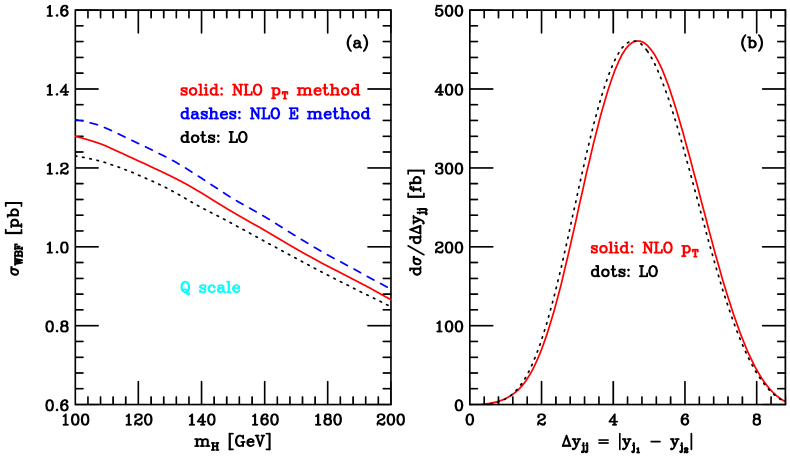
Figure 18: Effect of QCD radiative corrections on the Higgs boson production cross section via VBF. Results are given at LO (black dotted) and at NLO for the $p_{T}$ method (solid red) and the $E$ method (dashed blue) of defining tagging jets. Panel (a) gives the cross section within the cuts of Eqs. (3)–(6) as a function of the Higgs boson mass, $m_{H}$. Panel (b) shows the rapidity separation of the two tagging jets for $m_{H}=120$ GeV.

In order to reconstruct jets from final-state partons, the $k_{T}$ algorithm [92, 93, 94], as described in Ref. [95], is used, with resolution parameter $D=0.8$. We calculate the partonic cross sections for events with at least two hard jets, which are required to have

$$p_{Tj}\geq 20~{}{\rm GeV}\,,\qquad\qquad|y_{j}|\leq 4.5\,.$$ (3)

Here $y_{j}$ denotes the rapidity of the (massive) jet momentum which is reconstructed as the four-vector sum of massless partons of pseudorapidity $|\eta|<5$. The two reconstructed jets of highest transverse momentum are called “tagging jets” and are identified with the final-state quarks which are characteristic for vector-boson fusion processes. We call this method of choosing the tagging jets the “$p_{T}$ method”, as opposed to the “$E$ method” which identifies the two jets with the highest lab energy as tagging jets.

The Higgs boson decay products (generically called “leptons” in the following) are required to fall between the two tagging jets in rapidity and they should be well observable. While cuts for the Higgs boson decay products will depend on the channel considered, we here substitute such specific requirements by generating isotropic Higgs boson decay into two massless “leptons” (which represent $\tau^{+}\tau^{-}$ or $\gamma\gamma$ or $b\bar{b}$ final states) and require

$$p_{T\ell}\geq 20~{}{\rm GeV}\,,\qquad|\eta_{\ell}|\leq 2.5\,,\qquad\triangle R_{j\ell}\geq 0.6\,,$$ (4)

where $\triangle R_{j\ell}$ denotes the jet-lepton separation in the rapidity-azimuthal angle plane. In addition the two “leptons” are required to fall between the two tagging jets in rapidity

$$y_{j,min}<\eta_{\ell_{1,2}}<y_{j,max}\,.$$ (5)

When considering the decays $Z\to\ell^{+}\ell^{-}$ and $W\to\ell\nu$, we apply the same cuts of Eqs. (4) and (5) to the charged leptons (we have used here a slightly smaller jet-lepton separation $\triangle R_{j\ell}\geq 0.4$).

Backgrounds to vector-boson fusion are significantly suppressed by requiring a large rapidity separation of the two tagging jets (rapidity-gap cut)

$$\Delta y_{jj}=|y_{j_{1}}-y_{j_{2}}|>4\;.$$ (6)

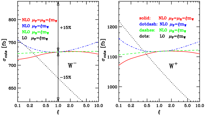
Figure 19: Scale dependence of the total cross section at LO and NLO within the cuts of Eqs. (3)–(6) for $W^{-}$ and $W^{+}$ production at the LHC. The factorization scale $\mu_{F}$ and/or the renormalization scale $\mu_{R}$ have been taken as multiples of the vector-boson mass, $\xi\,m_{W}$, and $\xi$ is varied in the range $0.1<\xi<10$. The NLO curves are for $\mu_{F}=\mu_{R}=\xi m_{W}$ (solid red line), $\mu_{F}=m_{W}$ and $\mu_{R}=\xi\,m_{W}$ (dashed green line) and $\mu_{R}=m_{W}$ and $\mu_{F}$ variable (dot-dashed blue line). The dotted black curve shows the dependence of the LO cross section on the factorization scale. At LO, $\alpha_{s}(\mu_{R})$ does not enter.

Cross sections, within the cuts of Eqs. (3)–(6), are shown in Fig. 18(a) as a function of the Higgs boson mass, $m_{H}$. As for the total VBF cross section, the NLO effects are modest for the cross section within cuts, amounting to a 3-5% increase for the $p_{T}$ method of selecting tagging jets and a 6-9% increase when the $E$ method is used. The differential cross section as function of the rapidity separation between the two tagging jets is plotted in Fig. 18(b). The wide separation of the tagging jets, which is important for rejection of QCD backgrounds, slightly increases at NLO. This example also shows that the $K$-factor, the ratio of NLO to LO differential cross sections, is strongly phase space dependent, i.e. an overall constant factor will not be adequate to simulate the data.

A comparison of our VBFNLO program with the MCFM Monte Carlo shows good agreement for predicted Higgs boson cross sections and also for those jet distributions which we have investigated. As an example, Table 3 shows cross sections within the cuts of Eqs. (3) and (6). No cuts on Higgs decay products are imposed because MCFM does not yet include Higgs boson decays. Cross sections agree at the 2% level or better, which is more than adequate for LHC applications. The results in the table were obtained with fixed scales $\mu_{R}=\mu_{F}=m_{H}$ and have Monte Carlo statistical errors of less than 0.5%.

Table 3: Higgs production cross sections (in pb) from MCFM and VBFNLO after jet cuts.

	mH (GeV)	100	120	140	160	180	200
$\sigma_{LO}$	MCFM	1.91	1.68	1.48	1.32	1.17	1.05
	VBFNLO	1.88	1.66	1.47	1.31	1.16	1.04
$\sigma_{NLO}$	MCFM	2.00	1.78	1.58	1.42	1.27	1.14
	VBFNLO	1.95	1.74	1.55	1.40	1.25	1.13

Cross sections for $W^{-}jj$ and $W^{+}jj$ production, within the cuts listed above, are shown in Fig. 19. In both panels, the scale dependence of cross sections is shown for fixed renormalization and factorization scales, $\mu_{R}=\xi_{R}\,m_{W}$ and $\mu_{F}=\xi_{F}\,m_{W}$. The LO cross sections only depend on $\mu_{F}$. At NLO we show three cases: (a) $\xi_{F}=\xi_{R}=\xi$ (red solid line); (b) $\xi_{F}=\xi$, $\xi_{R}=1$ (blue dot-dashed line); and (c) $\xi_{R}=\xi$, $\xi_{F}=1$ (green dashed line). While the factorization-scale dependence of the LO result is sizable, the NLO cross sections are quite insensitive to scale variations: allowing a factor 2 variation in either directions, i.e., considering the range $0.5<\xi<2$, the NLO cross sections change by less than 1% in all cases. Similar results were found for the VBF Higgs production cross section [89]. Alternative scale choices, like the virtuality of the exchanged electroweak bosons, also lead to cross sections changes of order 1-2% at NLO. Also for distributions, scale variations rarely exceed this range [89, 90]. These results indicate very stable NLO predictions for VBF cross sections with generic acceptance cuts.

In addition to these quite small scale uncertainties, we have estimated the error of the $Hjj$ and $W^{\pm}jj$ cross sections due to uncertainties in the determination of the PDFs, and we have found a total PDF uncertainty of $\pm 4\%$ with the CTEQ PDFs, and of roughly $\pm 2\%$ with the MRST set.

Summarizing, QCD corrections to distributions in VBF processes are in general of modest size, of order 10%, but occasionally they reach larger values. These corrections are strongly phase-space dependent for jet observables and an overall $K$-factor multiplying the LO distributions is not an adequate approximation. Within the phase-space region relevant for Higgs boson searches, we find differential $K$-factors as small as 0.9 or as large as 1.3. The residual combined QCD and PDF uncertainties of the NLO VBF cross sections are about 4%.

6 PDF uncertainties in Higgs production at the LHC

Parton distribution functions (PDFs), which describe the momentum distribution of a parton in the proton, play a central role at hadron colliders. A precise knowledge of the PDFs over a wide range of the proton momentum fraction $x$ carried by the parton and the squared centre-of-mass energy $Q^{2}$ at which the process takes place, is mandatory to precisely predict the production cross sections of the various signals and background hard processes. However, they are plagued by uncertainties, which arise either from the starting distributions obtained from a global fit to the available data from deep-inelastic scattering, Drell–Yan and hadronic data, or from the DGLAP evolution to the higher $Q^{2}$ relevant to the LHC scattering processes. Together with the effects of unknown perturbative higher order corrections, these uncertainties dominate the theoretical error on the predictions of the production cross sections.

PDFs with intrinsic uncertainties became available in 2002. Before that date, to quantitatively estimate the uncertainties due to the structure functions, it was common practice to calculate the production cross sections using the “nominal fits” or reference set of the PDFs provided by different parametrizations and to consider the dispersion between the various predictions as being the “uncertainty” due to the PDFs. However, the comparison between different parametrizations cannot be regarded as an unambiguous way to estimate the uncertainties since the theoretical and experimental errors spread into quantitatively different intrinsic uncertainties following their treatment in the given parametrization. The CTEQ and MRST collaborations and Alekhin recently introduced new schemes, which provide the possibility of estimating the intrinsic uncertainties and the spread uncertainties on the prediction of physical observables at hadron colliders.

In this short note, the spread uncertainties on the Higgs boson production cross sections at the LHC, using the CTEQ6 [96], MRST2001 [97] and ALEKHIN2002 [98] sets of PDFs, are investigated and compared. For more details, we refer to [99].

The scheme introduced by both the CTEQ and MRST collaborations is based on the Hessian matrix method. The latter enables a characterization of a parton parametrization in the neighbourhood of the global $\chi^{2}$ minimum fit and gives an access to the uncertainty estimation through a set of PDFs that describes this neighbourhood. Fixed target Drell–Yan data as well as $W$ asymmetry and jet data from the Tevatron are used in the fit procedure.

The corresponding PDFs are constructed as follows: (i) a global fit of the data is performed using the free parameters $N_{\rm PDF}=20$ for CTEQ and $N_{\rm PDF}=15$ for MRST; this provides the nominal PDF (reference set) denoted by $S_{0}$ and corresponding to CTEQ6M and MRST2001E, respectively; ( (ii) the global $\chi^{2}$ of the fit is increased by $\Delta\chi^{2}=100$ for CTEQ and $\Delta\chi^{2}=50$ for MRST, to obtain the error matrix [note that the choice of an allowed tolerance is only intuitive for a global analysis involving a number of different experiments and processes]; (iii) the error matrix is diagonalized to obtain $N_{\rm PDF}$ eigenvectors corresponding to $N_{\rm PDF}$ independent directions in the parameter space; (iv) for each eigenvector, up and down excursions are performed in the tolerance gap, leading to $2N_{\rm PDF}$ sets of new parameters, corresponding to 40 new sets of PDFs for CTEQ and 30 sets for MRST. They are denoted by $S_{i}$, with $i=1,2N_{\rm PDF}$.

To built the Alekhin PDFs [98], only light-target deep-inelastic scattering data [i.e. not the Tevatron data] are used. This PDF set involves 14 parameters, which are fitted simultaneously with $\alpha_{s}$ and the structure functions. To take into account the experimental errors and their correlations, the fit is performed by minimizing a $\chi^{2}$ functional based on a covariance matrix. Including the uncertainties on the $\alpha_{s}$ fit, one then obtains $2N_{\rm PDF}=30$ sets of PDFs for the uncertainty estimation.

These three sets of PDFs are used to calculate the uncertainty on a cross section $\sigma$ in the following way [99]: one first evaluates the cross section with the nominal PDF $S_{0}$ to obtain the central value $\sigma_{0}$. One then calculates the cross section with the $S_{i}$ PDFs, giving $2N_{\rm PDF}$ values $\sigma_{i}$, and defines, for each $\sigma_{i}$ value, the deviations $\Delta\sigma_{i}^{\pm}=\mid\sigma_{i}-\sigma_{0}\mid$ when $\sigma_{i}\ ^{>}{}_{<}\sigma_{0}$. The uncertainties are summed quadratically to calculate $\Delta\sigma^{\pm}=\sqrt{\sum_{i}\sigma_{i}^{\pm 2}}$. The cross section, including the error, is then given by $\sigma_{0}|^{+\Delta\sigma^{+}}_{-\Delta\sigma^{-}}$.

This procedure is applied to estimate the cross sections for the production of the Standard Model Higgs boson in the following four main mechanisms:

$${\rm associate~{}production~{}with}~{}W/Z: q\bar{q}\rightarrow VH$$ (7)

$${\rm massive~{}vector~{}boson~{}fusion}: qq\rightarrow Hqq$$ (8)

$${\rm the~{}gluon~{}gluon~{}fusion~{}mechanism}: gg\rightarrow H\hskip 56.9055pt$$ (9)

$${\rm associate~{}production~{}with~{}top~{}quarks}: gg,q\bar{q}\rightarrow t\bar{t}H$$ (10)

We will use the Fortran codes V2HV, VV2H, HIGLU and HQQ of Ref. [100] for the evaluation of the production cross sections of processes (1) to (4), respectively, at the LHC. A few remarks are to be made in this context: (i) the NLO QCD corrections to the Higgs-strahlung processes [101, 102] are practically the same for $WH$ and $ZH$ final states; we thus simply concentrate on the dominant $q\bar{q}\to WH$ process; the corrections to $qq\to Hqq$ have been obtained in Ref. [80, 89] (ii) for the gluon fusion process, $gg\to H$, we include the full dependence on the top and bottom quark masses of the NLO cross section [103] and not only the result in the infinite top quark mass limit [104]; (iii) for the $pp\to Ht\bar{t}$ production process, the NLO corrections have been calculated only recently [105] and the programs for calculating the cross sections are not yet publicly available. However, we choose a scale for which the LO and NLO cross sections are approximately equal and use the program HQQ for the LO cross section that we fold with the NLO PDFs; (iv) finally, we note that the NNLO corrections are also known in the case of $q\bar{q}\to HV$ [66] and $gg\to H$ [in the infinite top quark mass limit] [106] processes. We do not consider these higher order corrections since the CTEQ and MRST PDFs with errors are not available at this order.

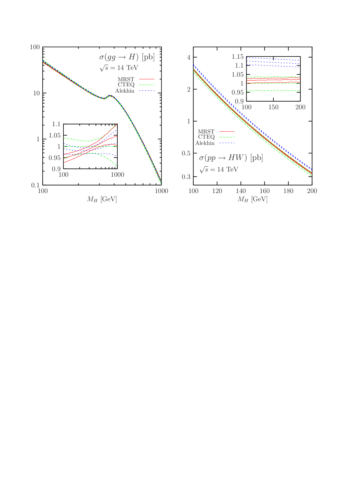
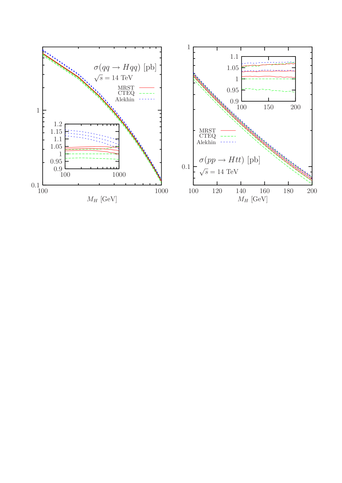
Figure 20: The CTEQ, MRST and Alekhin PDF uncertainty bands for the NLO cross sections for the production of the Higgs boson at the LHC in the four production processes. The insets show the spread in the predictions, when the NLO cross sections are normalized to the prediction of the reference CTEQ6M set.

The behaviour of the Higgs production cross sections and their uncertainties depends on the considered partons and their $x$ regime discussed above. In Fig. 20, we present the cross sections for the four production processes at the LHC. The central values and the uncertainty band limits of the NLO cross sections are shown for the CTEQ, MRST and Alekhin parameterizations. In the insets to these figures, we show the spread uncertainties in the predictions for the NLO cross sections, when they are normalized to the prediction of the reference CTEQ6M set. Note that the three sets of PDFs do not use the same value for $\alpha_{s}$: at NLO, the reference sets CTEQ6M, MRST2001C and A02 use, respectively, the values $\alpha_{s}^{\rm NLO}(M_{Z})=0.118$, $0.119$ and 0.117.

By observing Fig. 20, we see that the uncertainties for the Higgs cross sections obtained using the CTEQ6 set are two times larger than those using the MRST2001 sets. This is mainly due to two reasons: first, as noted previously, the CTEQ collaboration increased the global $\chi^{2}$ by $\Delta\chi^{2}=100$ to obtain the error matrix, while the MRST collaboration used only $\Delta\chi^{2}=50$; second, 2$\times$20 parameter uncertainties are summed quadratically in CTEQ6, while only 2$\times$15 are used in the MRST case. The uncertainties from the Alekhin PDFs are larger than the MRST ones and smaller than the CTEQ ones. In the subsequent discussion, the magnitude of the uncertainty band is expressed in terms of the CTEQ6 set.

$\bullet$ $q\bar{q}\rightarrow VH$: the uncertainty band is almost constant and is of the order of 4% [for CTEQ] over a Higgs masse range between 100 and 200 GeV. To produce a vector plus a Higgs boson in this mass range, the incoming quarks originate from the intermediate-$x$ regime. The different magnitude of the cross sections, $\sim 12$% larger in the Alekhin case than for CTEQ, is due to the larger quark and antiquark densities.

$\bullet$ $gg\rightarrow H$: the uncertainty band for the CTEQ set of PDFs decreases from the level of about 5% at $M_{H}\sim 100$ GeV, down to the 3% level at $M_{H}\sim$ 300 GeV. This is because Higgs bosons with relatively small masses are mainly produced by asymmetric low-$x$–high-$x$ gluons with a low effective c.m. energy; to produce heavier Higgs bosons, a symmetric process in which the participation of intermediate-$x$ gluons with high density, is needed, resulting in a smaller uncertainty band. At higher masses, $M_{H}\raisebox{-3.69899pt}{~{}\shortstack{$>$ \\ [-0.07cm] $\sim$}}~{}300$ GeV, the participation of high-$x$ gluons becomes more important, and the uncertainty band increases, to reach the 10% level at Higgs masses of about 1 TeV.

$\bullet$ $gg/q\bar{q}\rightarrow t\bar{t}H$: at the LHC, the associated production of the Higgs boson with a top quark pair is dominantly generated by the gluon–gluon fusion mechanism. Compared with the process $gg\rightarrow H$ discussed previously and for a fixed Higgs boson mass, a larger $Q^{2}$ is needed for this final state; the initial gluons should therefore have higher $x$ values. In addition, the quarks that are involved in the subprocess $q\bar{q}\rightarrow t\bar{t}H$, which is also contributing, are still in the intermediate regime because of the higher value $[x\sim 0.7$] at which the quark high-$x$ regime starts. This explains why the uncertainty band increases smoothly from 5% to 7% when the $M_{H}$ value increases from 100 to 200 GeV.

$\bullet$ $qq\rightarrow Hqq$: in the entire Higgs boson mass range from 100 GeV to 1 TeV, the incoming quarks involved in this process originate from the intermediate-$x$ regime and the uncertainty band is almost constant, ranging between 3% and 4%. When using the Alekhin set of PDFs, the behaviour is different, because the quark PDF behaviour is different, as discussed in the case of the $q\bar{q}\to HV$ production channel. The decrease in the central value with higher Higgs boson mass [which is absent in the $q\bar{q}\to HV$ case, since we stop the $M_{H}$ variation at 200 GeV] is due to the fact that we reach here the high-$x$ regime, where the Alekhin $\bar{u}$ PDF drops steeply.

In summary, we have considered three sets of PDFs with uncertainties provided by the CTEQ and MRST collaborations and by Alekhin. We evaluated their impact on the total cross sections at next-to-leading-order for the production of the Standard Model Higgs boson at the LHC. Within a given set of PDFs, the deviations of the cross sections from the values obtained with the reference PDF sets are rather small, ${\cal O}(5$%), in the case of the Higgs-strahlung, vector boson fusion and associated $t\bar{t}H$ production processes, but they can reach the level of 10% at the LHC in the case of the gluon–gluon fusion process for large enough Higgs boson masses, $M_{H}\sim 1$ TeV. However, the relative differences between the cross sections evaluated with different sets of PDFs can be much larger. Normalizing to the values obtained with the CTEQ6M set, for instance, the cross sections can be different by up to 15% for the four production mechanisms.

7 Measuring the Higgs Self-Coupling

7.1 Introduction

The LHC is widely regarded as capable of directly observing the agent responsible for electroweak symmetry breaking and fermion mass generation. This is generally believed to be a light Higgs boson with mass $m_{H}<219$ GeV [107]. The LHC will easily find a light Standard Model (SM) Higgs boson with very moderate luminosity [108, 109, 110, 111]. Moreover, the LHC will have significant capability to determine many of its properties [59, 60], such as its fermionic and bosonic decay modes and couplings [112, 113, 114, 115, 116, 79]. An $e^{+}e^{-}$ linear collider with a center of mass energy of 350 GeV or more can significantly improve these preliminary measurements, in some cases by an order of magnitude in precision, if an integrated luminosity of 500 fb^-1 can be achieved [117].

Perhaps the most important measurement after a Higgs boson discovery is of the Higgs potential itself, which requires measurement of the trilinear and quartic Higgs boson self-couplings. Only multiple Higgs boson production can probe these directly [118, 119, 120, 121, 122, 123, 124]. Phenomenologically one should write an effective Lagrangian that does not already assume SM couplings, as the object at hand could be a radion or other Higgs boson-like field that has different tree-level self-couplings. Only after the potential is measured can it be decided what the candidate actually is. We take the Lagrangian as the effective potential

$$V(\eta_{H})\,=\,{1\over 2}\,m_{H}^{2}\,\eta_{H}^{2}\,+\,\lambda\,v\,\eta_{H}^{3}\,+\,{1\over 4}\,\tilde{\lambda}\,\eta_{H}^{4},$$ (11)

where $\eta_{H}$ is the physical Higgs field, $v=(\sqrt{2}G_{F})^{-1/2}$ is the vacuum expectation value, and $G_{F}$ is the Fermi constant. In the SM,

$$\tilde{\lambda}=\lambda=\lambda_{SM}={m_{H}^{2}\over 2v^{2}}\,.$$ (12)

Since future collider experiments likely cannot probe $\tilde{\lambda}$, we concentrate on the trilinear coupling $\lambda$ in the following. The quartic Higgs coupling does not affect the Higgs pair production processes we consider.

There are numerous quantitative sensitivity limit analyses of Higgs boson pair production in $e^{+}e^{-}$ collisions ranging from 500 GeV to 3 TeV center of mass energies [120, 121, 122, 123, 124, 125]. In the past two years, several studies exploring the potential of the LHC, a luminosity-upgraded LHC (SLHC) with roughly ten times the amount of data expected in the first run, and a Very Large Hadron Collider (VLHC), were carried out [126, 127, 128, 129, 130, 131]. In the following we briefly summarize our [127, 128, 130, 131] studies of Higgs pair production at hadron colliders, concentrating on the LHC and SLHC, and compare the capabilities of future hadron and lepton colliders to measure $\lambda$. We also present a new estimate of the $t\bar{t}j$ background, and the results of a first study of how QCD corrections affect the signal in Higgs pair production for $m_{H}>140$ GeV.

7.2 Higgs Pair Production at Hadron Colliders

At LHC energies, inclusive Higgs boson pair production is dominated by gluon fusion [132, 133]. Other processes, such as weak boson fusion, $qq\to qqHH$ [134, 135, 136, 137], associated production with heavy gauge bosons, $q\bar{q}\to WHH,ZHH$ [138], or associated production with top quark pairs, $gg,\,q\bar{q}\to t\bar{t}HH$ [126], yield cross sections which are factors of 10–30 smaller than that for $gg\to HH$. Since $HH$ production at the LHC is generally rate limited, we consider only the gluon fusion process.

For $m_{H}<140$ GeV, the dominant decay mode of the SM Higgs boson is $H\to b\bar{b}$. In this region, the $b\bar{b}\gamma\gamma$ final state offers the best prospects to measure the Higgs self-coupling [131]; other final states such as $4b$, $b\bar{b}\tau^{+}\tau^{-}$ and $b\bar{b}\mu^{+}\mu^{-}$ are overwhelmed by backgrounds [130, 131].

For $m_{H}>140$ GeV, $H\to W^{+}W^{-}$ dominates, and the $W^{+}W^{-}W^{+}W^{-}$ final state has the largest individual branching ratio. Here, the $(jj\ell^{\pm}\nu)(jj{\ell^{\prime}}^{\pm}\nu)$ final state offers the best chance to extract information on $\lambda$ [126, 127, 128, 129].

7.2.1 $m_{H}<140$ GeV: The $b\bar{b}\gamma\gamma$ decay channel

The Feynman diagrams contributing to $gg\to HH$ in the SM consist of fermion triangle and box diagrams [118, 119]. Non-standard Higgs boson self-couplings only affect the triangle diagrams with a Higgs boson exchanged in the $s$-channel. We calculate the $gg\to HH\to b\bar{b}\gamma\gamma$ cross section using exact loop matrix elements [118, 119]. Signal results are computed consistently to leading order QCD with the top quark mass set to $m_{t}=175$ GeV and the renormalization and factorization scales are taken to be $m_{H}$. The effects of next-to-leading order (NLO) QCD corrections are included via a multiplicative factor $K=1.65$ [139].

The kinematic acceptance cuts for events are:

$$p_{T}(b)>45~{}{\rm GeV}\;,\qquad|\eta(b)|<2.5\;,\qquad\Delta R(b,b)>0.4\;,$$

$$m_{H}-20~{}{\rm GeV}\,<\,m_{b\bar{b}}\,<\,m_{H}+20~{}{\rm GeV}\;,$$

$$p_{T}(\gamma)>20~{}{\rm GeV}\;,\qquad|\eta(\gamma)|<2.5\;,\qquad 2.0>\Delta R(\gamma,\gamma)>0.4\;,\qquad\Delta R(\gamma,b)>1.0\;,$$

$$m_{H}-2.3~{}{\rm GeV}\,<\,m_{\gamma\gamma}\,<\,m_{H}+2.3~{}{\rm GeV}\;,$$

motivated by the requirement that the events can pass the ATLAS and CMS triggers with high efficiency [59, 60], and that the $b$-quark and photon pairs reconstruct to windows around the known Higgs boson mass. We take the identification efficiency for each photon to be $80\%$ and assume that $b$-quarks are tagged with an efficiency of $\epsilon_{b}=50\%$. The $\Delta R(\gamma,\gamma)$ and $\Delta R(\gamma,b)$ cuts help to reduce the background such that $S/B\sim 1/2$ (1/1) is possible at the LHC (SLHC) [131].

The only irreducible background processes are QCD $b\bar{b}\gamma\gamma$, $H(\to\gamma\gamma)b\bar{b}$ and $H(\to b\bar{b})\gamma\gamma$ production. However, there are multiple QCD reducible backgrounds resulting from jets faking either $b$-jets or photons, such as 4 jet production (one or two fake $b$-jets, two fake photons) or $b\bar{b}j\gamma$ production (one fake photon) [131]. We simulate these backgrounds assuming a misidentification probability of light jets as $b$-quarks of $P_{j\to b}=1/140$ (1/23) at the LHC (SLHC), and a jet – photon misidentification probability in the range $1/2500<P_{j\to\gamma}<1/1600$. With these parameters, most of the background originates from reducible sources.

Almost all reducible backgrounds depend on whether one requires one or both $b$-quarks to be tagged. Requiring only one tagged $b$-quark results in a signal cross section which is a factor $(2/\epsilon_{b}-1)=3$ larger than the one with both $b$-quarks tagged. This larger signal rate comes at the expense of a significantly increased reducible background. The small $gg\to HH\to b\bar{b}\gamma\gamma$ rate forces us to require only a single $b$-tag at the LHC in order to have an observable signal. At the SLHC, on the other hand, the much higher probability to misidentify a light jet as a $b$-jet translates into an increase of the background which more than compensates the signal gain from using only a single $b$-tag. In the following we therefore require a double $b$-tag at the SLHC.

To discriminate between signal and background, we use the visible invariant mass, $m_{\rm vis}$, which for this final state is the invariant mass of the Higgs boson pair, corrected for energy loss of the $b$-jets. We show this in Fig. 21 for $m_{H}=120$ GeV at the LHC and SLHC.

Figure 21: The visible invariant mass distribution, $m_{\rm vis}$, in $pp\to b\bar{b}\gamma\gamma$, after all kinematic cuts, for the QCD backgrounds (long dashed) and a SM signal of $m_{H}=120$ GeV (solid) at the LHC and SLHC. We assume $P_{j\to\gamma}=1/2500$ in the background calculation. The dotted and short dash-dotted lines show the signal cross section for $\lambda_{HHH}=\lambda/\lambda_{SM}=0$ and 2, respectively.

Performing a $\chi^{2}$ test of the $m_{\rm vis}$ distribution, one finds the following $1\sigma$ sensitivity bounds for $m_{H}=120$ GeV:

$$-1.1<\Delta\lambda_{HHH}<1.6 {\rm LHC~{}600~{}fb}^{-1},$$ (13)

$$-0.62<\Delta\lambda_{HHH}<0.74 {\rm SLHC~{}6000~{}fb}^{-1},$$ (14)

where $\Delta\lambda_{HHH}=\lambda/\lambda_{SM}-1$. For $m_{H}=140$ GeV, the SLHC could obtain bounds which are about a factor 2 weaker than those for $m_{H}=120$ GeV; there are not enough signal events at the LHC to derive sensitivity limits for $m_{H}=140$ GeV. If the photon–jet and light jet–$b$ misidentification probabilities can be independently measured in other processes, one can subtract large parts of the reducible backgrounds which do not involve charm quarks. This may improve the sensitivity limits by a factor $1.5-2$. Due to the small number of events, the LHC and SLHC sensitivity limits depend significantly on the SM cross section normalization uncertainty. The bounds listed in Eqs. (13) and (14) have been calculated assuming a normalization uncertainty of $10\%$ for the SM (signal plus background) cross section. This depends critically on knowledge of the signal QCD corrections and the ability to determine the background normalization. The NLO QCD corrections to $gg\to HH$ are currently known only in the infinite top quark mass limit [139]. To ensure the $10\%$ required precision on differential cross sections we would need the NLO rates for finite top quark masses, as well as the NNLO corrections at least in the heavy top quark mass limit. For the background normalization one can either rely on calculations of the QCD corrections (which do not exist yet) or perform a sideband analysis of the data.

We should compare the bounds listed in Eqs. (13) and (14) with those achievable at $e^{+}e^{-}$ linear colliders. A linear collider with $\sqrt{s}=500$ GeV and an integrated luminosity of 1 ab^-1 can determine $\lambda$ with a precision of about $20\%$ ($50\%$) in $e^{+}e^{-}\to ZHH$ for $m_{H}=120(140)$ GeV [125, 130]. From Eq. (13) it is clear that the LHC will be able to provide only a first rough measurement of the Higgs self-coupling for $m_{H}=120$ GeV. The SLHC would be able to make a more precise measurement. However, the sensitivity bounds on $\lambda$ obtained from $b\bar{b}\gamma\gamma$ production for $m_{H}=120(140)$ GeV will be a factor 2 – 4 (1.2 – 3) weaker than those achievable at a linear collider. Although a luminosity-upgraded LHC cannot compete with a linear collider for Higgs masses $m_{H}<140$ GeV, a Higgs self-coupling measurement at the SLHC would still be interesting if realized before a linear collider begins operation.

We finally note that the $b\bar{b}\gamma\gamma$ final state is particularly interesting in the MSSM framework, because it is the only channel in which we can hope to observe a heavy Higgs state for small values of $\tan\beta$. However, we do not include any detailed analysis, because the MSSM search strategy does not differ significantly from the SM case described below.

7.2.2 $m_{H}>140$ GeV: The same sign dilepton channel

A thorough analysis of $gg\to HH\to(W^{+}W^{-})(W^{+}W^{-})\to(jj\ell^{\pm}\nu)(jj{\ell^{\prime}}^{\pm}\nu)$ was presented in Refs. [127, 128]. After a brief review of the main results of this analysis, we present a reevaluation of the $t\bar{t}j$ background and the results of a preliminary study of how initial state gluon radiation affects the $m_{vis}$ distribution of the signal which is used to extract limits on $\lambda$.

In our analysis [127, 128], we perform the calculation of the $gg\to HH\to(W^{+}W^{-})(W^{+}W^{-})\to(jj\ell^{\pm}\nu)(jj{\ell^{\prime}}^{\pm}\nu)$ signal cross section as in Sec. 7.2.1. The kinematic acceptance cuts are:

$$p_{T}(j)>30,\,30,\,20,\,20~{}{\rm GeV},\qquad p_{T}(\ell)>15,\,15~{}{\rm GeV},$$ (15)

$$|\eta(j)|<3.0,\qquad\qquad\qquad\qquad|\eta(\ell)|<2.5,$$ (16)

$$\Delta R(jj)>1.0,\qquad\Delta R(j\ell)>0.4,\qquad\Delta R(\ell\ell)>0.2.$$ (17)

In addition we require the four jets to combine into two pseudo-$W$ pairs with invariant masses $50~{}{\rm GeV}<m(jj)<110~{}{\rm GeV}$, and assume that this captures $100\%$ of the signal and backgrounds. We do not impose a missing transverse momentum cut which would remove a considerable fraction of the signal events; it is unnecessary for this analysis.

The relevant SM backgrounds are those that produce two same-sign leptons and four well-separated jets which reconstruct to two pairs, each in a window around the $W$ boson mass. The largest contribution originates from $W^{\pm}W^{+}W^{-}jj$ production (which includes $W^{\pm}H(\to W^{+}W^{-})jj$), followed by $t\bar{t}W^{\pm}$ where one top quark decays leptonically, the other hadronically, and neither $b$ quark jet is tagged. Other backgrounds are: $W^{\pm}W^{\pm}jjjj$; $t\bar{t}t\bar{t}$, where none of the $b$ quark jets are tagged, and additional jets or leptons are not observed; $W^{\pm}Zjjjj$, $t\bar{t}Z$ and $W^{+}W^{-}Zjj$ with leptonic $Z$ decay (including off-shell photon interference) where one lepton is not observed; and $t\bar{t}j$ events where one $b$ quark decays semileptonically with good hadronic isolation and the other is not tagged. In Ref. [128] we found that the $t\bar{t}j$ channel contributes $10\%$ or less of the total background.

To discriminate signal from background we again use the $m_{vis}$ distribution, i.e. the distribution of the $\ell^{\pm}{\ell^{\prime}}^{\pm}+4j$ invariant mass, which we show for $m_{H}=180$ GeV in Fig. 22a.

Figure 22: a) The $m_{vis}$ distribution of the signal for $pp\to\ell^{\pm}{\ell^{\prime}}^{\pm}+4j$ and $m_{H}=180$ GeV at the LHC, in the SM (solid curve), for $\lambda_{HHH}=\lambda/\lambda_{SM}=0$ (dashed line) and for $\lambda_{HHH}=2$ (dotted line). The dot-dashed line shows the combined $m_{vis}$ distribution of all background processes. We obtain qualitatively similar results for other values of $m_{H}$.
b) Limits achievable at $95\%$ CL for $\Delta\lambda_{HHH}=(\lambda-\lambda_{SM})/\lambda_{SM}$ in $pp\to\ell^{\pm}{\ell^{\prime}}^{\pm}+4j$ at the (S)LHC. Bounds are shown for integrated luminosities of 300 fb^-1 (solid lines), 600 fb^-1 (dashed lines) and 3000 fb^-1 (dotted lines). The allowed region is between the two lines of equal texture. The Higgs boson self-coupling vanishes for $\Delta\lambda_{HHH}=-1$. The figures are taken from Ref. [128].

The background distribution peaks at a significantly higher value than the signal. Performing a $\chi^{2}$ test for the $m_{vis}$ distribution, we find the $95\%$ CL limits shown in Fig. 22b. The results of Ref. [127, 128] demonstrate that, with 300 fb^-1 at the LHC, one will be able to perform a first, albeit not very precise, measurement of the Higgs boson self-coupling. The non-vanishing of $\lambda$, however, can be established at $95\%$ CL or better for $150~{}{\rm GeV}\lesssim m_{H}\lesssim 200$ GeV. This alone is an important, non-trivial test of spontaneous symmetry breaking; the exact non-zero value of $\lambda$ may vary depending on the way nature chooses to spontaneously break the electroweak symmetry. At the SLHC, for 3000 fb^-1, a measurement with a precision of up to $20\%$ at $95\%$ CL would be possible; the SLHC could determine $\lambda$ with an accuracy of $10-30\%$ at the $1\sigma$ level for Higgs boson masses between 150 and 200 GeV.

Due to phase space restrictions, a center of mass energy of at least 800 GeV would be needed to search for Higgs pair production in $e^{+}e^{-}$ collisions if $m_{H}\geq 150$ GeV. For $\sqrt{s}=0.8-1$ TeV, $e^{+}e^{-}\to ZHH\to 10~{}{\rm jets},\,\ell\nu+8~{}{\rm jets}$ via Higgs boson decays into weak boson pairs are the dominant Higgs pair production channels. The main contributions to the background originate from $t\bar{t}\>+$ jets and $WW+$ jets production, with cross sections several orders of magnitude larger than the signal. As a result, it will be difficult to determine the Higgs boson self-coupling at a linear collider with $\sqrt{s}=0.8-1$ TeV with a precision equal to that which can be reached at the LHC with 300 fb^-1 [130].

7.2.3 Toward a more complete simulation of the $(jj\ell^{\pm}\nu)(jj{\ell^{\prime}}^{\pm}\nu)$ channel

In Ref. [128], the $t\bar{t}j$ background was estimated from a parton level calculation which took only $b\to c\ell\nu$ decays into account; $b\to u\ell\nu$ decays were ignored. Furthermore, the $\chi^{2}$ analysis used to extract sensitivity bounds for $\lambda$ in Ref. [127, 128] assumed that higher order QCD corrections do not significantly alter the shape of the $m_{vis}$ distribution for signal and background. In the following, we present a new estimate of the $t\bar{t}j$ background which includes the contribution from $b\to u\ell\nu$ decays and address the question of how higher order QCD corrections change the shape of the $m_{vis}$ distribution of the signal.

Re-evaluation of the $t\bar{t}j$ background

Since the $t\bar{t}j$ cross section is several orders of magnitude larger than the $HH$ signal, it is crucial to suppress it sufficiently. This is accomplished by requiring isolation of the lepton originating from semileptonic $b$-decay. Due to phase space restrictions, the $t\bar{t}j$ background is extremely sensitive to the $p_{T}(\ell)$ cut and the lepton isolation criteria. A typical lepton isolation cut limits the energy fraction carried by the charm or $u$-quark from $b$-decay in a cone around the lepton, or imposes an upper limit on its transverse momentum. It is easy to show [140] that, for $b\to c\ell\nu$ decays, the kinematics limits the transverse momentum of the lepton to

$$p_{T}(\ell)\leq{m_{B}^{2}\over m_{D}^{2}}~{}p_{Tmax}(c),$$ (18)

where $p_{Tmax}(c)$ is the maximal transverse momentum of the charm quark allowed in the isolation cone, and $m_{B}$ and $m_{D}$ are the $B$ and $D$ meson masses which are used to approximately obtain the correct kinematics. In Ref. [128], $p_{Tmax}(c)=3$ GeV and a cone size of $\Delta R=0.4$ were used, implying that $p_{T}(\ell)<24$ GeV. The large suppression of the $t\bar{t}j$ background noted in our previous analysis, and its extreme dependence on the $p_{T}(\ell)$ cut, thus is entirely due to phase space suppression. In fact, for $p_{Tmax}(c)=1$ GeV which was used in Ref. [129], the $t\bar{t}j$ cross section would vanish for the cuts listed in Eq. (15).

From Eq. (18) it is obvious that the phase space is much less suppressed for $b\to u\ell\nu$ decays. There, $m_{D}$ in Eq. (18) has to be replaced by either the $\pi$ or $\rho$ mass, allowing much larger lepton transverse momenta. Although $b\to u\ell\nu$ decays are suppressed by the ratio $(V_{ub}/V_{cb})^{2}\approx 8\times 10^{-3}$ with respect to $b\to c\ell\nu$, there are regions of phase space where contributions from $b\to u\ell\nu$ decays dominate over those from $b\to c\ell\nu$ in the $t\bar{t}j$ background.

We estimate the $t\bar{t}j$ background with $b\to u\ell\nu$ decays using the approach described in Ref. [128], the measured $B\to\pi\ell\nu$ branching fractions [141], and assuming that all remaining $b\to u\ell\nu$ decays result in final state hadrons with an invariant mass $\geq m_{\rho}$. Taking into account the uncertainties in $V_{ub}$ ($V_{ub}=0.0036\pm 0.0007$ [141]) we find, imposing the cuts listed in Eqs. (15) and (17),

$$\sigma(t\bar{t}j,b\to u\ell\nu)=0.76\pm 0.28~{}{\rm fb}$$ (19)

if one requires $p_{T}(u)<3$ GeV in a cone of $\Delta R=0.4$ around the charged lepton. This should be compared with $\sigma(t\bar{t}j,b\to c\ell\nu)=0.08$ fb for $p_{T}(c)<3$ GeV obtained in Ref. [128]. Taking into account $b\to u\ell\nu$ decays thus increases the $t\bar{t}j$ background cross section by a factor $6-12$ and the total background by a factor $1.4-2.2$. This is expected to weaken the limits on $\lambda$ by a factor $1.2-1.4$. If the $p_{T}$ threshold is lowered to $p_{T}(u)<1$ GeV, one finds $\sigma(t\bar{t}j,b\to u\ell\nu)=0.33\pm 0.12$ fb. In this case the sensitivity limits worsen by a factor 1.2 at most.

We also note that the $t\bar{t}j$, $b\to u\ell\nu$ background cross section significantly depends on the size of the cone used in the isolation of the lepton. Reducing the cone size from $\Delta R=0.4$ to $\Delta R=0.2$, for example, increases the $t\bar{t}j$ cross section by approximately a factor 6 for $p_{T}(u)<1$ GeV. On the other hand, if the isolation cone is increased to $\Delta R=0.5$, the $t\bar{t}j$ cross section is reduced by a factor 2.

The cross sections for the $t\bar{t}j$ background listed in Eq. (19) assume vertex tagging of the hadronically decaying $b$-quark, rejecting events with a factor 2, which approximates the fraction where the $b$-quark would be tagged. We made no such assumption for the semileptonically decaying $b$. Requiring a small impact parameter for the lepton originating from $b$-decay may result in an additional suppression of the $t\bar{t}j$ background.

We emphasize that our matrix element-based estimate of the $t\bar{t}j$ background should be viewed with some caution. Our treatment of the phase space in $b\to u\ell\nu$ clearly is oversimplified. Furthermore, effects from hadronization, event pileup and extra jets from initial or final state radiation, as well as detector resolution effects may significantly affect the rejection. For a reliable estimate of the background, a full detector simulation is required, which is best carried out by interfacing a matrix element based calculation of $t\bar{t}j$ production with an event generator such as pythia. This is now underway.

Initial state gluon radiation in $HH$ production

To investigate how extra jets from initial state gluon radiation affect the shape of the $m_{vis}$ distribution of the signal, we used an interface of the hpair program with pythia [142]. The results for $m_{H}=200$ GeV are shown in Fig. 23.

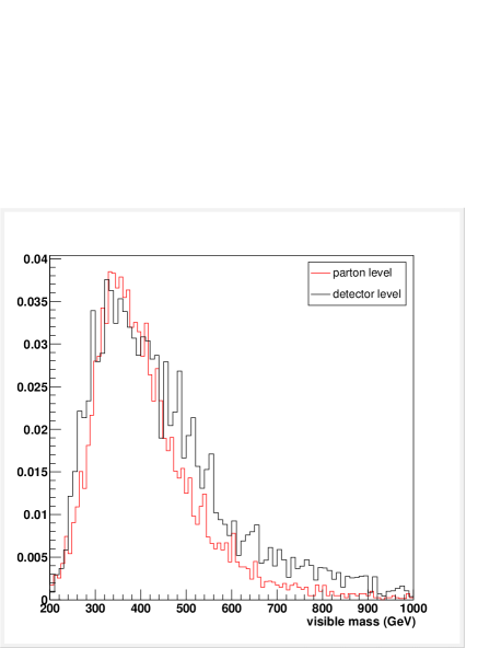
Figure 23: The $m_{vis}$ distribution for $gg\to HH+X\to(jj\ell^{\pm}\nu)(jj{\ell^{\prime}}^{\pm}\nu)+X$ with $m_{H}=200$ GeV at the LHC obtained from interfacing the hpair program with pythia. The red histogram (“parton level”) shows the result obtained using the momenta of the four jets from $W$ decays in calculating the visible invariant mass. In the black histogram, the momenta of the four jets with the highest transverse momenta in the event are used in computing $m_{vis}$. The units on the vertical axis are arbitrary.

The red histogram, labeled “parton level”, displays the result obtained when the momenta of the four jets which originate from $W$ decays are used to calculate $m_{vis}$, and corresponds to the result of a lowest order calculation. For the black histogram, the momenta of the four jets with the highest transverse momenta in the event are used to compute $m_{vis}$. Frequently, one of these jets originates from initial state gluon radiation. Fig. 23 demonstrates that, while QCD corrections broaden the $m_{vis}$ distribution somewhat, the location of the peak and the shape of the distribution remain essentially unchanged.

Similar calculations have to be carried out for the main background channels, $WWWjj$ and $t\bar{t}W$ production, before firm conclusions how QCD corrections affect the sensitivity limits for $\lambda$ can be drawn.

7.3 Conclusions

After discovery of an elementary Higgs boson and tests of its fermionic and gauge boson couplings, experimental evidence that the shape of the Higgs potential has the form required for electroweak symmetry breaking will complete the proof that fermion and weak boson masses are generated by spontaneous symmetry breaking. One must determine the Higgs self-coupling to probe the shape of the Higgs potential.

Only Higgs boson pair production at colliders can accomplish this. Numerous studies [120, 121, 122, 123, 124, 125] have established that future $e^{+}e^{-}$ machines can measure $\lambda$ at the $20-50\%$ level for $m_{H}<140$ GeV. A recent study has shown that a measurement of the Higgs self-coupling at a luminosity upgraded LHC in this mass range using the $b\bar{b}\gamma\gamma$ final state is also possible. Although the SLHC cannot compete with a linear collider in this mass range, a Higgs self-coupling measurement at the SLHC will still be interesting if realized before a linear collider begins operation.

While a measurement of the Higgs self-coupling at a linear collider for $m_{H}>140$ GeV requires a center of mass energy larger than 1 TeV [143], the LHC may rule out the case of vanishing $\lambda$ for $150~{}{\rm GeV}<m_{H}<200$ GeV at $95\%$ CL. At the SLHC, for 3000 fb^-1, a measurement with a precision of up to $20\%$ at $95\%$ CL is possible. These sensitivity limits were derived from a parton level analysis of the visible invariant mass distribution in $pp\to\ell^{\pm}{\ell^{\prime}}^{\pm}+4j$. Major uncertainties in this analysis are the size of the $t\bar{t}j$ background and how initial state gluon radiation affects the $m_{vis}$ distribution. First, but still preliminary, results indicate that the shape of the signal $m_{vis}$ distribution is broadened slightly by QCD corrections. Since $b\to u\ell\nu$ decays were originally neglected, the $t\bar{t}j$ background was underestimated by a factor $3-6$ in Ref. [128]. This is expected to weaken the sensitivity bounds on $\lambda$ by up to $20\%$. A more complete calculation of the $t\bar{t}j$ background, including detector effects, is needed before realistic sensitivity limits for the Higgs self-coupling at the LHC for $m_{H}>140$ GeV can be obtained.

8 Charged Higgs Production via $bg\longrightarrow tH^{-}$

8.1 Introduction

The Minimal Supersymmetric Standard Model (MSSM) introduces charged Higgs bosons in addition to the Standard Model neutral Higgs boson. The discovery of the Higgs is one of the main aims of the current Run II at the Tevatron and the future program at the LHC. The charged Higgs would be an important signal of new physics beyond the Standard Model.

An important partonic channel for charged Higgs discovery at hadron colliders is associated production with a top quark via bottom-gluon fusion, $bg\longrightarrow tH^{-}$. The complete next-to-leading order (NLO) corrections to this process have been studied in Refs. [144, 145]. Here, I discuss soft-gluon corrections to charged Higgs production, which are expected to be important near threshold, the kinematical region where the charged Higgs may be discovered at the LHC. Threshold corrections have been shown to be important for many processes in hadron colliders [146, 147, 148, 149, 150, 151, 152].

In the next section I first discuss the NLO soft-gluon corrections for $bg\longrightarrow tH^{-}$, and then I present the NNLO corrections at next-to-leading logarithmic (NLL) accuracy.

8.2 Threshold NNLO-NLL Corrections

For the process $b(p_{b})+g(p_{g})\rightarrow t(p_{t})+H^{-}(p_{H})$, we define the kinematical invariants $s=(p_{b}+p_{g})^{2}$, $t=(p_{b}-p_{t})^{2}$, $u=(p_{g}-p_{t})^{2}$, and $s_{4}=s+t+u-m_{t}^{2}-m_{H}^{2}$, where $m_{H}$ is the charged Higgs mass, $m_{t}$ is the top quark mass, and we ignore the bottom quark mass $m_{b}$. Note that near threshold, i.e. when we have just enough partonic energy to produce the $tH^{-}$ final state, $s_{4}\rightarrow 0$. Threshold corrections appear as $[\ln(s_{4}/m_{H}^{2})/s_{4}]_{+}$.

The differential Born cross section is $d^{2}{\hat{\sigma}}^{bg\rightarrow tH^{-}}_{B}/(dt\;du)=F^{bg\rightarrow tH^{-}}_{B}\delta(s_{4})$ where

$$F^{bg\rightarrow tH^{-}}_{B} = \frac{\pi\alpha\alpha_{s}(m_{b}^{2}\tan^{2}\beta+m_{t}^{2}\cot^{2}\beta)}{12s^{2}m_{W}^{2}\sin^{2}\theta_{W}}\left\{\frac{s+t-m_{H}^{2}}{2s}\right.$$ (20)

$$\left.{}-\frac{m_{t}^{2}(u-m_{H}^{2})+m_{H}^{2}(t-m_{t}^{2})+s(u-m_{t}^{2})}{s(u-m_{t}^{2})}-\frac{m_{t}^{2}(u-m_{H}^{2}-s/2)+su/2}{(u-m_{t}^{2})^{2}}\right\}\,,$$

where $\alpha_{s}$ is the strong coupling, $\alpha=e^{2}/(4\pi)$, $\tan\beta=v_{2}/v_{1}$ is the ratio of the vacuum expectation values of the two Higgs doublets in the MSSM, and we have kept $m_{b}$ non-zero only in the coupling.

The NLO soft-gluon corrections for $bg\rightarrow tH^{-}$ are

$$\frac{d^{2}{\hat{\sigma}}^{(1)}_{bg\rightarrow tH^{-}}}{dt\,du}=F^{bg\rightarrow tH^{-}}_{B}\frac{\alpha_{s}(\mu_{R}^{2})}{\pi}\left\{c^{bg\rightarrow tH^{-}}_{3}\left[\frac{\ln(s_{4}/m_{H}^{2})}{s_{4}}\right]_{+}+c^{bg\rightarrow tH^{-}}_{2}\left[\frac{1}{s_{4}}\right]_{+}+c^{bg\rightarrow tH^{-}}_{1}\delta(s_{4})\right\}\,.$$ (21)

Here $c^{bg\rightarrow tH^{-}}_{3}=2(C_{F}+C_{A})$, where $C_{F}=(N_{c}^{2}-1)/(2N_{c})$ and $C_{A}=N_{c}$ with $N_{c}=3$ the number of colors, and

$$c^{bg\rightarrow tH^{-}}_{2} = 2{\rm Re}{\Gamma^{\prime}}_{S}^{(1)}-C_{F}-C_{A}-2C_{F}\ln\left(\frac{-u+m_{H}^{2}}{m_{H}^{2}}\right)-2C_{A}\ln\left(\frac{-t+m_{H}^{2}}{m_{H}^{2}}\right)$$ (22)

$$-(C_{F}+C_{A})\ln\left(\frac{\mu_{F}^{2}}{s}\right)\equiv T^{bg\rightarrow tH^{-}}_{2}-(C_{F}+C_{A})\ln\left(\frac{\mu_{F}^{2}}{m_{H}^{2}}\right)\,,$$

where $\mu_{F}$ is the factorization scale, and we have defined $T^{bg\rightarrow tH^{-}}_{2}$ as the scale-independent part of $c^{bg\rightarrow tH^{-}}_{2}$. The term ${\rm Re}{\Gamma^{\prime}}_{S}^{(1)}=C_{F}\ln[(-t+m_{t}^{2})/(m_{t}\sqrt{s})]+(C_{A}/2)\ln[(-u+m_{t}^{2})/(-t+m_{t}^{2})]+C_{A}/2$ denotes the real part of the one-loop soft anomalous dimension, which describes noncollinear soft-gluon emission [153, 154, 155]. Also $c^{bg\rightarrow tH^{-}}_{1}=[C_{F}\ln((-u+m_{H}^{2})/m_{H}^{2})+C_{A}\ln((-t+m_{H}^{2})/m_{H}^{2})-3C_{F}/4-\beta_{0}/4]\ln(\mu_{F}^{2}/m_{H}^{2})+(\beta_{0}/4)\ln(\mu_{R}^{2}/m_{H}^{2})$, where $\mu_{R}$ is the renormalization scale and $\beta_{0}=(11C_{A}-2n_{f})/3$ is the lowest-order $\beta$ function, with $n_{f}=5$ the number of light quark flavors. Note that $c^{bg\rightarrow tH^{-}}_{1}$ represents the scale-dependent part of the $\delta(s_{4})$ corrections. We do not calculate the full virtual corrections here. Our calculation of the soft-gluon corrections includes the leading and next-to-leading logarithms (NLL) of $s_{4}$ and is thus a NLO-NLL calculation.

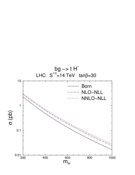
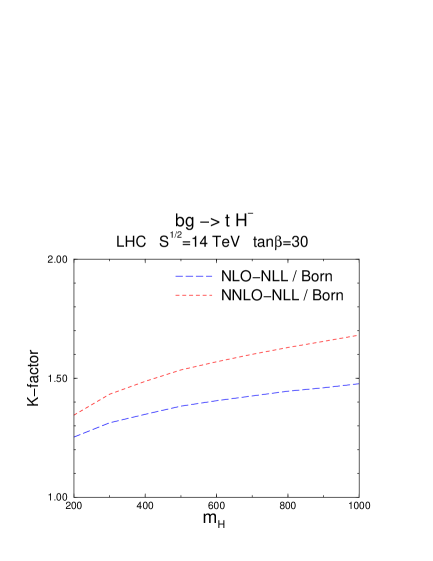
Figure 24: Charged Higgs production at the LHC. Left: The total cross section. Right: The $K$-factors.

We next calculate the NNLO soft-gluon corrections for $bg\rightarrow tH^{-}$ using the methods and master formulas of Ref. [156]:

$$\frac{d^{2}{\hat{\sigma}}^{(2)}_{bg\rightarrow tH^{-}}}{dt\,du}=F^{bg\rightarrow tH^{-}}_{B}\frac{\alpha_{s}^{2}(\mu_{R}^{2})}{\pi^{2}}\left\{\frac{1}{2}\left(c^{bg\rightarrow tH^{-}}_{3}\right)^{2}\left[\frac{\ln^{3}(s_{4}/m_{H}^{2})}{s_{4}}\right]_{+}\right.$$

$${}+\left[\frac{3}{2}c^{bg\rightarrow tH^{-}}_{3}\,c^{bg\rightarrow tH^{-}}_{2}-\frac{\beta_{0}}{4}c^{bg\rightarrow tH^{-}}_{3}\right]\left[\frac{\ln^{2}(s_{4}/m_{H}^{2})}{s_{4}}\right]_{+}$$

$${}+\left[c^{bg\rightarrow tH^{-}}_{3}\,c^{bg\rightarrow tH^{-}}_{1}+(C_{F}+C_{A})^{2}\ln^{2}\left(\frac{\mu_{F}^{2}}{m_{H}^{2}}\right)-2(C_{F}+C_{A})T_{2}^{bg\rightarrow tH^{-}}\ln\left(\frac{\mu_{F}^{2}}{m_{H}^{2}}\right)\right.$$

$$\quad\left.{}+\frac{\beta_{0}}{4}c^{bg\rightarrow tH^{-}}_{3}\ln\left(\frac{\mu_{R}^{2}}{m_{H}^{2}}\right)-\zeta_{2}\,\left(c^{bg\rightarrow tH^{-}}_{3}\right)^{2}\right]\left[\frac{\ln(s_{4}/m_{H}^{2})}{s_{4}}\right]_{+}$$

$${}+\left[-(C_{F}+C_{A})\ln\left(\frac{\mu_{F}^{2}}{m_{H}^{2}}\right)c^{bg\rightarrow tH^{-}}_{1}-\frac{\beta_{0}}{4}(C_{F}+C_{A})\ln\left(\frac{\mu_{F}^{2}}{m_{H}^{2}}\right)\ln\left(\frac{\mu_{R}^{2}}{m_{H}^{2}}\right)\right.$$

$$\quad\left.\left.{}+(C_{F}+C_{A})\frac{\beta_{0}}{8}\ln^{2}\left(\frac{\mu_{F}^{2}}{m_{H}^{2}}\right)-\zeta_{2}\,c^{bg\rightarrow tH^{-}}_{2}\,c^{bg\rightarrow tH^{-}}_{3}+\zeta_{3}\,\left(c^{bg\rightarrow tH^{-}}_{3}\right)^{2}\right]\left[\frac{1}{s_{4}}\right]_{+}\right\}\,,$$ (23)

where $\zeta_{2}=\pi^{2}/6$ and $\zeta_{3}=1.2020569...$. We note that only the coefficients of the leading ($\ln^{3}$) and next-to-leading logarithms ($\ln^{2}$) of $s_{4}$ are complete. Hence this is a NNLO-NLL calculation. Consistent with a NLL calculation we have also kept all logarithms of the factorization and renormalization scales in the $[\ln(s_{4}/m_{H}^{2})/s_{4}]_{+}$ terms, and squares of scale logarithms in the $[1/s_{4}]_{+}$ terms, as well as $\zeta_{2}$ and $\zeta_{3}$ terms that arise in the calculation of the soft corrections.

We now convolute the partonic cross sections with parton distribution functions (we use MRST2002 NNLO  [34]) to obtain the hadronic cross section in $pp$ collisions at the LHC. We use $\mu_{F}=\mu_{R}=m_{H}$ for our numerical results. In the left frame of Fig. 24 we plot the cross section for charged Higgs production at the LHC with $\sqrt{S}=14$ TeV versus the charged Higgs mass. We use $m_{t}=175$ GeV, $m_{b}=4.5$ GeV, and $\tan\beta=30$. The Born, NLO-NLL, and NNLO-NNLL results are shown. Both the NLO and the NNLO threshold corrections are important as can be more clearly seen in the right frame of Fig. 24 where we plot the $K$-factors, i.e. the ratios of the NLO-NLL over Born and the NNLO-NLL over Born cross sections. As expected, the corrections increase for larger charged Higgs mass since then we get closer to threshold. Finally, we note that the cross section for ${\bar{b}}g\longrightarrow{\bar{t}}H^{+}$ is the same as for $bg\longrightarrow tH^{-}$.

8.3 Conclusion

The soft-gluon threshold corrections for the process $bg\longrightarrow tH^{-}$ have been calculated through next-to-next-to-leading order and next-to-leading logarithmic accuracy. We have seen that numerically both the NLO and NNLO threshold corrections to charged Higgs production at the LHC are important.

9 FeynHiggs 2.1: High Precision Calculations in the MSSM Higgs Sector

9.1 Introduction

The search for the lightest Higgs boson is a crucial test of Supersymmetry (SUSY) which can be performed with the present and the next generation of accelerators. Especially for the Minimal Supersymmetric Standard Model (MSSM) a precise prediction for the masses of the Higgs bosons and their decay widths to other particles in terms of the relevant SUSY parameters is necessary in order to determine the discovery and exclusion potential of the upgraded Tevatron, and for physics at the LHC and future linear colliders.

In the case of the MSSM with complex parameters (cMSSM) the task is even more involved. Several parameters can have non-vanishing phases. In particular, these are the Higgs mixing parameter, $\mu$, the trilinear couplings, $A_{f}$, $f=t,b,\tau,\ldots$, and the gaugino masses $M_{1}$, $M_{2}$, and $M_{3}\equiv m_{\tilde{g}}$ (the gluino mass). Furthermore the neutral Higgs bosons are no longer ${\cal CP}$-eignestates, but mix with each other once loop corrections are taken into account [157].

$$(h,H,A)\to h_{1},h_{2},h_{3}~{}~{}~{}{\rm with}~{}~{}~{}m_{h_{1}}\leq m_{h_{2}}\leq m_{h_{3}}\,.$$ (24)

The input parameters within the Higgs sector are then (besides the Standard Model (SM) ones) $\tan\beta$, the ratio of the two vacuum expectation values, and the mass of the charge Higgs boson, $M_{H^{\pm}}$.

9.2 The Code FeynHiggs 2.1

FeynHiggs 2.1 [158] is a Fortran code for the evaluation of masses and mixing angles in the MSSM with real or complex parameters. The calculation of the higher-order corrections is based on the Feynman-diagrammatic (FD) approach [159]. At the one-loop level, it consists a complete evalutaion, including the full momentum dependence. The renormalization has been performed in a hybrid $\overline{\rm{MS}}$ /on-shell scheme [160]. At the two-loop level all existing corrections from the real MSSM have been included (see Ref. [161] for a review). They are supplemented by the resummation of the leading effects from the (scalar) $b$ sector including the full complex phase dependence.

Besides the evaluation of the Higgs-boson masses and mixing angles, the program also includes the evaluation of all relevant Higgs-boson decay widths. These are in particular:

• the total width for the three neutral and the charged Higgs boson,

• the BR’s of the Higgs bosons to SM fermions (see also Ref. [162]), ${\rm BR}(h_{i}\to f\bar{f})$, ${\rm BR}(H^{+}\to f\bar{f}^{\prime})$,

• the to SM gauge bosons (possibly off-shell), ${\rm BR}(h_{i}\to\gamma\gamma,ZZ^{*},WW^{*},gg)$,

• the decay into gauge and Higgs bosons, ${\rm BR}(h_{i}\to Zh_{j})$, ${\rm BR}(h_{i}\to h_{j}h_{k})$, ${\rm BR}(H^{+}\to h_{i}W^{+})$,

• the decay to scalar fermions, ${\rm BR}(h_{i}\to\tilde{f}\bar{\tilde{f}})$, ${\rm BR}(H^{+}\to\tilde{f}\bar{\tilde{f}^{\prime}})$,

• the decay of the Higgs bosons to gauginos, ${\rm BR}(h_{i}\to\chi^{\pm}_{k}\chi^{\mp}_{j})$, ${\rm BR}(h_{i}\to\chi^{0}_{l}\chi^{0}_{m})$,
  ${\rm BR}(H^{+}\to\chi^{+}_{k}\chi^{0}_{l})$.

For comparisons with the SM the following quantities are also evaluated for SM Higgs bosons with the same mass as the three neutral MSSM Higgs bosons:

• the total decay widths,

• the BR’s of a SM Higgs boson to SM fermions,

• the BR’s of a SM Higgs boson to SM gauge bosons (possibly off-shell).

In addition, the following couplings and cross sections are evaluated

• the coupling of Higgs and gauge bosons, $g_{VVh_{i}}$, $g_{Vh_{i}h_{j}}$,

• the Higgs-boson self couplings, $g_{h_{i}h_{j}h_{k}}$,

• the Higgs-boson production cross section at a $\gamma\gamma$ collider, $\sigma(\gamma\gamma\to h_{i})$.

Finally as external constraints are evaluated

• the $\rho$-parameter up to the two-loop level [163] that indicates disfavored scalar top and bottom masses

• the anomalous magnetic moment of the muon, including a full one-loop calculation as well as leading and subleading two-loop corrections [164].

Comparing our results to existing codes like Hdecay [165] (for the real case) or CPsuperH [166] (for the cMSSM), we find differences in the mass evaluations for the lightest Higgs boson of ${\cal O}(4\,\,\mathrm{GeV})$. These are due to the inclusion of higher-order corrections in FeynHiggs 2.1 that shift the lightest Higgs-boson mass upwards. Concerning the BR evaluation (and compensating for the effects from the different Higgs-boson masses) we find quantitative and qualitative agreement. For more details see Ref. [158].

FeynHiggs 2.1 possesses some further features that can be summarizes as,

• transformation of the input parameters from the $\overline{\rm{DR}}$ to the on-shell scheme (for the scalar top and bottom parameters), including the full ${\cal O}(\alpha_{s})$ and ${\cal O}(\alpha_{t,b})$ corrections.

• processing of Les Houches Accord (LHA) data [167]. FeynHiggs 2.1 reads the output of a spectrum generator file and evaluates the Higgs boson masses, brachning ratios etc. The results are written in the LHA format to a new output file.

• the SPS benchmark scenarios [168] and the Les Houches benchmarks for Higgs boson searches at hadron colliders [169] are given as a possibly predefined input

• detailed information about all the features of FeynHiggs 2.1 (see also the next section) are provided in man pages.

9.3 How to install and use FeynHiggs 2.1

To take advantage of all features of FeynHiggs 2.1, the LoopTools library [170] needs to be installed, which can be obtained from www.feynarts.de/looptools. Without this library, FeynHiggs 2.1 will still compile, but not all branching ratios will be available.

• Download the package from www.feynhiggs.de.

• Say ./configure and make. This creates libFH.a and the command-line frontend.

• To build also the Mathematica frontend, say make all.

There are three different ways to use FeynHiggs 2.1.

9.3.1 The Fortran library

The libFH.a library can be linked directly to other Fortran programs. To avoid naming conflicts, all externally visible symbols have been prefixed with “fh.” No include files are needed since the user calls only subroutines (no functions). Detailed descriptions of the invocations of the subroutines are given in the respective man pages.

9.3.2 The command-line frontend

The FeynHiggs executable is a command-line frontend to the libFH.a library. It reads the parameters from an ASCII input file and writes the output in a human-readable form to the screen. Alternatively, this output can be piped through a filter to yield a machine-readable version appropriate for plotting etc. The parameter file is fairly flexible and allows to define also loops over parameters. Also the Les-Houches-Accord file format can be read and written.

9.3.3 The Mathematica frontend

The MFeynHiggs executable provides access to the libFH.a functions from Mathematica via the MathLink protocol. This is particularly convenient both because FeynHiggs 2.1 can be used interactively this way and because Mathematica’s sophisticated numerical and graphical tools, e.g. FindMinimum, are available.

10 Mass Bounds for a SU(2) Triplet Higgs

10.1 Introduction

The precision high–energy measurements of electoweak observables by LEP, SLC and Tevatron have confirmed the Glashow–Salam–Weinberg model to a great certainty. The remaining challenge is to pin down the nature of the breaking of the electroweak symmetry. If it occurs via the Standard Model Higgs mechanism, with a complex isospin doublet, the mass of the lightest Higgs is $81^{+52}_{-33}$ GeV [171], with similar bounds for the simplest supersymmetric models. In this contribution we present the study of a simple extension of the Standard Model where the new feature is the addition of a real Higgs triplet. This model is compatible with precision measurements as will be shown below, and allows for the lightest Higgs boson mass to go up to about 500 GeV. This review is based on the work in Ref. [172, 173].

10.2 The Triplet Higgs Model

The lagrangian of the model in terms of the usual Standard Model Higgs, $\Phi_{1}$, and the new triplet, $\Phi_{2}$, reads

$${\cal L}=(D_{\mu}\Phi_{1})^{\dagger}D^{\mu}\Phi_{1}+\frac{1}{2}(D_{\mu}\Phi_{2})^{\dagger}D^{\mu}\Phi_{2}-V_{0}(\Phi_{1},\Phi_{2})\,,$$

with a scalar potential $V_{0}(\Phi_{1},\Phi_{2})=\mu_{1}^{2}|\Phi_{1}|^{2}+\frac{\mu_{2}^{2}}{2}|\Phi_{2}|^{2}+\lambda_{1}|\Phi_{1}|^{4}+\frac{\lambda_{2}}{4}|\Phi_{2}|^{4}+\frac{\lambda_{3}}{2}|\Phi_{1}|^{2}|\Phi_{2}|^{2}+\lambda_{4}\,{\Phi_{1}}^{\dagger}\sigma^{\alpha}\Phi_{1}{\Phi_{2}}_{\alpha}$. $\sigma^{\alpha}$ are the Pauli matrices. The expansion of the field components is

$$\Phi_{1}=\begin{pmatrix}\phi^{+}\cr\frac{1}{\sqrt{2}}\left(h_{c}^{0}+h^{0}+i\phi^{0}\right)\end{pmatrix}_{Y=1}\,,\qquad\Phi_{2}=\begin{pmatrix}\eta_{1}\cr\eta_{2}\cr\eta_{c}^{0}+\eta^{0}\end{pmatrix}_{Y=0}$$

where $\eta^{\pm}=(\eta_{1}\mp i\eta_{2})/\sqrt{2}$ and $\phi^{0}$ is the Goldstone boson which is eaten by the $Z^{0}$. In the neutral Higgs sector we have two CP-even states which mix with angle $\gamma$. The mass eigenstates $\{H^{0},N^{0}\}$ are

$$\begin{pmatrix}H^{0}\cr N^{0}\end{pmatrix}=\begin{pmatrix}\cos{\gamma}&-\sin{\gamma}\cr\sin{\gamma}&\cos{\gamma}\end{pmatrix}\begin{pmatrix}h^{0}\cr\eta^{0}\end{pmatrix}.$$

There is also mixing in the charged Higgs sector. We define the mass eigenstates $\{g^{\pm},h^{\pm}\}$ by

$$\begin{pmatrix}g^{\pm}\cr h^{\pm}\end{pmatrix}=\begin{pmatrix}\cos{\beta}&-\sin{\beta}\cr\sin{\beta}&\cos{\beta}\end{pmatrix}\begin{pmatrix}\phi^{\pm}\cr\eta^{\pm}\end{pmatrix}.$$

The $g^{\pm}$ are the Goldstone bosons corresponding to $W^{\pm}$ and, at tree level, the mixing angle is $\tan{\beta}=2\frac{\eta^{0}_{c}}{h^{0}_{c}}$. The model violates custodial symmetry at tree level giving a prediction for the $\rho$-parameter of $\rho=1+4\left(\frac{\eta^{0}_{c}}{h^{0}_{c}}\right)^{2}$. We will show below how it is precisely this violation of custodial symmetry what allows for the mass of the lightest Higgs to be large in this model.

10.3 Comparison with Data from oblique Corrections

Predictions for the oblique corrections to EW observables can be written in terms of the $S$, $T$ and $U$ parameters which can quantify the effect of varying the Higgs mass. The TM contributions, to leading order in $\beta$, are [172]

$$S_{TM} = 0,$$

$$T_{TM} = \frac{1}{8\pi}\,\frac{1}{s^{2}_{W}c^{2}_{W}}\left[\frac{m^{2}_{N^{0}}+m^{2}_{h^{\pm}}}{m^{2}_{Z}}\;-\;\frac{2m^{2}_{h^{\pm}}m^{2}_{N^{0}}}{m^{2}_{Z}(m^{2}_{N^{0}}-m^{2}_{h^{\pm}})}\log\left(\frac{m^{2}_{N^{0}}}{m^{2}_{h^{\pm}}}\right)\right]\simeq\frac{1}{6\pi}\,\frac{1}{s^{2}_{W}c^{2}_{W}}\;\frac{(\Delta m)^{2}}{m^{2}_{Z}}.$$

$$U_{TM} = -\frac{1}{3\pi}\left(m_{N^{0}}^{4}\log\left(\frac{m_{N^{0}}^{2}}{m_{h^{\pm}}^{2}}\right)\frac{(3m_{h^{\pm}}^{2}-m_{N^{0}}^{2})}{(m_{N^{0}}^{2}-m_{h^{\pm}}^{2})^{3}}+\frac{5(m_{N^{0}}^{4}+m_{h^{\pm}}^{4})-22m_{N^{0}}^{2}m_{h^{\pm}}^{2}}{6(m_{N^{0}}^{2}-m_{h^{\pm}}^{2})^{2}}\right)+O\left(\frac{m_{Z}}{m_{h^{\pm}}}\right)$$

$$\simeq \frac{\Delta m}{3\pi m_{h^{\pm}}}.$$

The TM contribution to $S$ is zero to this order since $Y=0$. Apart from the loop correction, there is also a tree level contribution which arises in all observables as a result of the tree level deviation of the rho parameter from unity. This contribution leads effectively to a positive contribution to T. The TM contribution to $T$ is positive and, in the approximation of $\Delta m=m_{N^{0}}-m_{h^{\pm}}\ll m_{h^{\pm}}$, has the rough power dependence shown above. $U$ also vanishes when $\Delta m\to 0$, and falls to zero at large triplet masses. In particular, it has a negligible effect on all the results we shall subsequently show provided $m_{N^{0}},\,m_{h^{\pm}}>1$ TeV.

Figure 25: Ellipse encloses the region allowed by data. Left: Curves show results in the TM for various values of $\beta$ and various doublet Higgs masses with $\Delta m=0$ and $U=0$. Right: Curves show results in the TM for various mass splittings and various doublet Higgs masses with $\beta$ and $U$ assumed to be negligible.

Using the program ZFITTER [174] we compute a total of 13 standard observables [171] with $m_{h}^{ref}=100~{}{\rm GeV}$, $m_{t}=174.3$ GeV, $G_{\mu}=1.16639\times 10^{-5}$ GeV^-2, $m_{Z}=91.1875$ GeV, $\alpha_{s}=$0.119 and $\Delta\alpha_{had}^{(5)}(m_{Z})$= 0.02804. These results then determine the allowed region in $S$–$T$ parameter space. This is represented by the interior of the ellipses shown in Fig. 25 (the ellipse corresponds to a 95$\%$ confidence limit).

In Fig. 25 (left) each line shows the TM at a particular value of $\beta$ for $\Delta m=0$ (which turns off the quantum corrections) and $m_{h}$ varying from 200 GeV to 2 TeV. We see that even in the absence of quantum corrections the TM is able to accommodate any $m_{h}$ up to 2 TeV and the mixing angle $\beta$ must be less than 0.07. In Fig. 25 (right) each line shows the TM result as $m_{h}$ is varied, as before, at fixed $\Delta m$. $\beta$ is assumed to be negligibly small in this plot (which turns off the tree-level correction) and as a result the $\Delta m=0$ line is identical to that which would arise in the SM. Clearly the quantum corrections contribute to $T$ so as to allow any $m_{h}$ up to 2 TeV and the mass splitting $\Delta m$ must be less than 125 GeV.

10.4 Renormalisation Group Evolution

We would like to examine the RG flow of the couplings and hence establish bounds on the scalar masses under the assumption that the triplet model remain perturbative and have a stable vacuum up to some scale $\Lambda=1$ TeV.

In Ref. [173] the beta functions for the couplings were calculated using the one–loop effective potential [175, 176, 177, 178, 179, 180] with $\overline{\rm MS}$ renormalization in ’t Hooft-Landau gauge and the anomalous dimensions for $h^{0}$ and $\eta^{0}$, the results read

$$\beta_{\mu_{1}} = \frac{1}{16\pi^{2}}\,\left(6\,\lambda_{4}^{2}+12\,\lambda_{1}\mu_{1}^{2}+3\,\lambda_{3}\,\mu_{2}^{2}\right)+\frac{1}{8\pi^{2}}\,\left(3\,h_{t}^{2}-\frac{9}{4}\,g^{2}-\frac{3}{4}\,{g^{\prime}}^{2}\right)\,\mu_{1}^{2},$$

$$\beta_{\mu_{2}} = \frac{1}{16\pi^{2}}\,\left(4\,\lambda_{4}^{2}+4\,\lambda_{3}\,\mu_{1}^{2}+10\,\lambda_{2}\,\mu_{2}^{2}\right)-\frac{3}{4\pi^{2}}\,g^{2}\,\mu_{2}^{2},$$

$$\beta_{\lambda_{1}} = \frac{1}{8\pi^{2}}\left(\frac{9}{16}\,g^{4}-3\,{{h_{t}}}^{4}+12\,\lambda_{1}^{2}+\frac{3}{4}\,\lambda_{3}^{2}+\frac{3}{8}\,g^{2}\,{g^{\prime}}^{2}+\frac{3}{16}\,{g^{\prime}}^{4}\right)$$

$$+ \frac{1}{4\pi^{2}}\,\left(3\,h_{t}^{2}-\frac{9}{4}\,g^{2}-\frac{3}{4}\,{g^{\prime}}^{2}\right)\,\lambda_{1},$$

$$\beta_{\lambda_{2}} = \frac{1}{8\pi^{2}}\left(6\,g^{4}+11\,\lambda_{2}^{2}+\lambda_{3}^{2}\right)-\frac{3}{2\pi^{2}}\,g^{2}\,\lambda_{2},$$

$$\beta_{\lambda_{3}} = \frac{1}{8\pi^{2}}\left(3\,g^{4}+6\,\lambda_{1}\,\lambda_{3}+5\,\lambda_{2}\,\lambda_{3}+2\,\lambda_{3}^{2}\right)+\frac{3\lambda_{3}}{8\pi^{2}}\,\left(h_{t}^{2}-\frac{11}{4}\,g^{2}-\frac{1}{4}\,{g^{\prime}}^{2}\right),$$

$$\beta_{\lambda_{4}} = \frac{1}{4\pi^{2}}\,\lambda_{4}\,\left(\lambda_{1}+\lambda_{3}\right)+\frac{3}{32\pi^{2}}\,\left(4\,h_{t}^{2}-7\,g^{2}-\,{g^{\prime}}^{2}\right)\,\lambda_{4}.$$

In the gauge and top quark sector the beta functions for the $U(1)$, $SU(3)$ and Yukawa couplings are the same as in the Standard Model and only the $SU(2)$ coupling is modified due to the extra Higgs triplet in the adjoint representation, i.e. $\beta_{g}=-\frac{5}{32\pi^{2}}\,g^{3}$.

Working with the tree-level effective potential with couplings evolved using the one-loop $\beta$ and $\gamma$ functions we are able to resum the leading logarithms to all orders in the effective potential. To carry out the RG analysis we first introduce the parameter $t$, related to $\mu$ through $\mu(t)=m_{Z}\exp{(t)}$. The RG equations are coupled differential equations in the set $\left\{g_{s},~{}g,~{}g^{\prime},~{}h_{t},~{}\mu_{1},~{}\mu_{2},~{}\lambda_{1},~{}\lambda_{2},~{}\lambda_{3},~{}\lambda_{4}\right\}$. We choose rather to use the set of variables $\left\{\alpha_{s},~{}m_{Z},~{}\sin^{2}{\theta_{W}},~{}m_{t},~{}m_{h^{\pm}},~{}m_{H^{0}},~{}m_{N^{0}},~{}v,~{}\tan{\beta},~{}\tan{\gamma}\right\}$.

Within the accuracy to which we are working, the values of the couplings at $t=0$ can be obtained from the input set using the appropriate tree–level expressions. Inverting the tree level relations for the masses we can fix the $t=0$ boundary conditions for the subsequent evolution. To ensure that the system remains in a local minimum we impose the condition that the squared masses should remain positive. We also impose that the couplings remain perturbative, insisting that $|\lambda_{i}(t)|<4\pi$ for $i={1,2,3}$ and $|\lambda_{4}|<4\pi v$. We run the evolution from $t=0$ to $t_{\rm max}=\log{(\Lambda/m_{Z})}$, with $\Lambda=1$ TeV.

In the non-decoupling regime the triplet cannot be arbitrarily heavy. In Fig. 26 (left) we show the range of Higgs masses allowed when there is no mixing in the neutral Higgs sector, $\gamma=0$, for $\beta=0.04$. Such a value is interesting because it allows a rather heavy lightest Higgs, e.g. for $\beta=0.04,\;m_{H^{0}}>150$ GeV and for $\beta=0.05,\;m_{H^{0}}>300$ GeV (see Fig. 25 (left) where $\Delta m\sim 0$ and the perturbativity of $\lambda_{2}$ implies negligible quantum corrections). The strong correlation between the $h^{\pm}$ and $N^{0}$ masses arises in order that $\lambda_{2}$ remain perturbative. The upper bound on the triplet Higgs masses ($\approx 550$ GeV) comes about from the perturbativity of $\lambda_{3}$ whilst that on $H^{0}$ ($\approx 520$ GeV) comes from the perturbativity of $\lambda_{1}$. The hole at low masses is due to vacuum stability. The non–zero $\gamma$ case has been considered in Ref. [172].

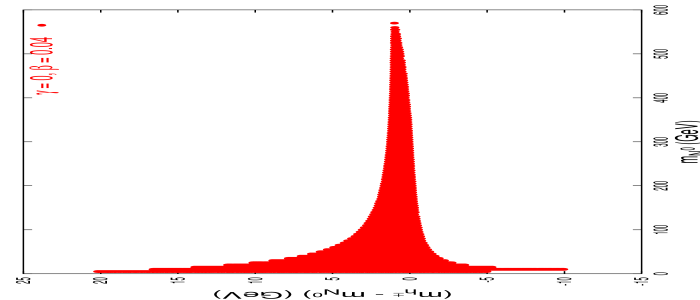
Figure 26: Allowed values of scalar masses for $\gamma=0$

For $\beta=\gamma=0$ there is no doublet-triplet mixing and no bound on the triplet mass. This is a special case of the more general decoupling scenario, which occurs when $|\beta+\gamma|\ll\beta$. For small mixing angles, the triplet Higgs has mass squared $\sim\lambda_{4}v/\beta$ and it is possible to have $\lambda_{4}\sim v$ by keeping $\mu_{2}^{2}$ large. In this case $\beta+\gamma\approx 0$. This is the decoupling limit in which the triplet mass lies far above the mass of the doublet and the low energy model looks identical to the Standard Model.

10.5 Conclusions

We have shown that it is quite natural in the triplet model for the lightest Higgs boson to have a mass as large as 500 GeV. Through an analysis of the oblique corrections it is possible to see that the model is compatible with precision electroweak data. Through a computation of the one–loop beta functions for the scalar couplings, and considerations of perturbativity of the couplings and vacuum stability we have identified the allowed masses of the Higgs bosons in the non-decoupling regime. In the decoupling regime, the model resembles the SM. The near degeneracy of the triplet Higgs masses ensures that, at least for small $\gamma$, the quantum corrections to the $T$ parameter are negligible (the $S$ parameter vanishing since the triplet has zero hypercharge). This means that the lightest Higgs boson can have a mass as large as 500 GeV as a result of the compensation arising from the explicit tree-level violation of custodial symmetry. Since the hypercharge of the triplet is zero, there are no associated problems with unwanted phenomenology and thus it is possible to be in a regime where all the scalars are $\sim 500$ GeV without any other deviation from the Standard Model.

11 W⁺W⁺ Scattering as a Sensitive Test of the Anomalous Gauge Couplings of the Higgs Boson at the LHC

The electroweak symmetry breaking mechanism (EWSBM) is one of the most profound puzzles in particle physics. Since the Higgs sector of the standard model (SM) suffers the well-known problems of triviality and unnaturalness , there has to be new physics beyond the SM above certain high energy scale $\Lambda$. If a light Higgs boson candidate ($H$) is found in future collider experiments, the next important task is to experimentally measure the gauge interactions of this Higgs scalar and explore the nature of the EWSBM. Let $~{}V=W^{\pm},~{}Z^{0}~{}$ be the electroweak (EW) gauge bosons. The detection of the anomalous $HVV$ couplings (AHVVC) will point to new physics beyond the SM underlying the EWSBM.

Figure 27: Illustration of Feynman diagrams for $VV$ scatterings in the SM: (a) diagrams contributing to $T(V,\gamma)$, (b) diagrams contributing to $T(H)$.

Before knowing the correct new physics, the effect of new physics at energy below $\Lambda$ can be parametrized as effective operators in an effective theory. This is a model-independent description. Testing the AHVVC relative to that of the SM can discriminate the EWSBM in the new physics model from that of the SM. In Ref. [181], we propose a sensitive way of testing the AHVVC via $VV$ scatterings, especially the $W^{+}W^{+}$ scatterings, at the LHC [181]. This includes the test of either the dim-3 AHVVC in a nonlinearly realized Higgs model (NRHM) [182] or the dim-6 AHVVC in the linearly realized effective interactions (LREI) [183]. The reason for the sensitiveness is the following. The scattering amplitude contains two parts: (i) the amplitude $T(V,\gamma)$ related only to $V$ and $\gamma$ (Fig. 1(a)), and (ii) the amplitude $T(H)$ related to the Higgs boson (Fig. 1(b)). At high energies, both $T(V,\gamma)$ and $T(H)$ increase with the center-of-mass energy ($E$) as $E^{2}$ in the NRHM and as $E^{4}$ in the LREI. In the SM, though individual diagrams in Fig. 1(a) may behave as $E^{4}$, the sum of all diagrams in Fig. 1(a) can have at most $E^{2}$-dependent contribution. The $HVV$ coupling constant in the SM is just the non-Abelian gauge coupling constant. This causes the two $E^{2}$-dependent pieces to precisely cancel with each other in $T(V,\gamma)+T(H)$, resulting in the expected $E^{0}$-behavior for the total amplitude, as required by the unitarity of the $S$ matrix. If there is AHVVC due to new physics effect, $T(V,\gamma)+T(H)$ can grow as $E^{2}$ or $E^{4}$ in the high energy regime. Such deviations from the $E^{0}$ behavior of the SM amplitude can provide a rather sensitive test of the AHVVC in high energy $VV$ scattering experiments. This type of tests do not require the measurement of the $H$ decay branching ratios, and is thus of special interest, especially if the AHVVC are very large or very small [181].

We take such enhanced $VV$ scatterings as the signals for testing the AHVVC. To avoid the large hadronic backgrounds at the LHC [185], We choose the gold-plated pure leptonic decay modes of the final state $V$s as the tagging modes. Even so, there are still several kinds of backgrounds to be eliminated [186, 187]. We take all the kinematic cuts given in Ref. [187] to suppress the backgrounds, and calculate the complete tree level contributions to the process

$$pp\mbox{$\rightarrow$}VVjj\mbox{$\rightarrow$}llll(\nu\nu)jj,$$ (25)

where $j$ is the forward jet that is tagged to suppress the large background rates. Our calculation shows that, for not too small AHVVC, all the backgrounds can be reasonably suppressed by such kinematic cuts. In the case of the SM, there are still considerably large remaining backgrounds contributed by the transverse component $V_{T}$. We shall call these the remaining SM backgrounds (RSMB) after taking the above treatment. Our calculation shows that the signals can be considerably larger than the RSMB even with not very large AHVVC.

We first consider the NRHM. The effective Lagrangian below $\Lambda$, up to dim-4 operators, respecting the EW gauge symmetry, charge conjugation, parity, and the custodial $SU(2)_{c}$ symmetry, is [182]:.

$${\cal L} = -{1\over 4}{\overrightarrow{W}}_{\mu\nu}\cdot{\overrightarrow{W}}^{\mu\nu}-{1\over 4}B_{\mu\nu}B^{\mu\nu}+{1\over 4}(v^{2}+2\kappa vH+\kappa^{\prime}H^{2}){\rm Tr}(D_{\mu}\Sigma^{\dagger}D^{\mu}\Sigma)$$ (26)

$$+{1\over 2}\partial_{\mu}H\partial^{\mu}H-{m_{H}^{2}\over 2}H^{2}-{\lambda_{3}v\over 3!}H^{3}+{\lambda_{4}\over 4!}H^{4},$$

where $\overrightarrow{W}_{\mu\nu}$ and $B_{\mu\nu}$ are field strengths of the EW gauge fields, $v\simeq 246$ GeV is the vacuum expectation value (VEV) breaking the EW gauge symmetry, $(\kappa,\,\lambda_{3})$ and $(~{}\kappa^{\prime},\,\lambda_{4})$ are, respectively, dimensionless coupling constants from the dim-3 and dim-4 operators, $\Sigma=\exp\{i{\overrightarrow{\tau}}\cdot{\overrightarrow{\omega}}/{v}\}$, and $~{}D_{\mu}\Sigma=\partial_{\mu}\Sigma+ig{\overrightarrow{\tau}\over 2}\cdot{\overrightarrow{W}}_{\mu}\Sigma-ig^{\prime}B_{\mu}\Sigma{\tau_{3}\over 2}$. The SM corresponds to $\kappa=\kappa^{\prime}=1$ and $\displaystyle\lambda_{3}=\lambda_{4}=\lambda={3m_{H}^{2}}/{v^{2}}$.

At the tree level, only the dim-3 operator ${1\over 2}\kappa vHD_{\mu}\Sigma^{\dagger}D^{\mu}\Sigma$ contributes to the $VV$ scatterings in Fig. 1. Therefore, $VV$ scatterings can test $\kappa$, and $\Delta\kappa\equiv\kappa-1$ measures the deviation from the SM value $\kappa=1$.

In Ref. [181], the full tree level cross sections for all the processes in (25) are calcuated for $115~{}{\rm GeV}\leq m_{H}\leq 300$ GeV. The results show that the most sensitive channel is  $pp\mbox{$\rightarrow$}W^{+}W^{+}jj\mbox{$\rightarrow$}l^{+}\nu l^{+}\nu jj$ [181]. With an integrated luminosity of 300 fb^-1, there are more than 20 events for $\Delta\kappa\geq 0.2$ or $\Delta\kappa\leq-0.3$, while there are only about 15 RSMB events (see Ref. [181] for details). Considering only the statistical errors, the LHC can limit $\Delta\kappa$ to the range

$$-0.3<\Delta\kappa<0.2$$ (27)

at roughly the $(1-3)\sigma$ level if data is consistent with the SM prediction [181].

Other constraints on $\Delta\kappa$ from the precision EW data, the requirement of the unitarity of the $S$-matrix, etc. were studied in Ref. [181], which are either weaker than Eq. (27) or of the similar level [181].

Next, we consider the LREI. In this theory, the leading AHVVC are from the effective operators of dim-6 [183, 184]. As is shown in Refs. [183, 184], the C and P conserving effective Lagrangian up to dimension-6 operators containing a Higgs doublet $\Phi$ and the weak bosons $V^{a}$ is given by

$${\cal L}_{\mbox{eff}}~{}\,=~{}\,\sum_{n}{f_{n}\over\Lambda^{2}}{\cal O}_{n}\,,$$ (28)

where ${\cal O}_{n}$’s are dim-6 operators composed of $\Phi$ and the EW gauge fields (cf. Ref. [184]), $f_{n}/\Lambda^{2}$’s are the AHVVC.

The precision EW data and the requirement of the unitarity of the $S$-matrix give certain constraints on the $f_{n}$’s. The constraints on $f_{WWW}/\Lambda^{2}$, $f_{WW}/\Lambda^{2}$, $f_{BB}/\Lambda^{2}$, $f_{W}/\Lambda^{2}$, and $f_{B}/\Lambda^{2}$ from the presently available experimental data are rather weak [181]. A better test of them is to study the $VV$ scatterings. In ${\cal L}_{\mbox{eff}}$, the operator ${\cal O}_{WWW}$ contributes to the triple and quartic $V$ boson self-interactions which may not be directly related to the EWSBM, we assume $f_{WWW}/\Lambda^{2}$ is small in the analysis. and concentrate on the test of $f_{WW}/\Lambda^{2}$, $f_{BB}/\Lambda^{2}$, $f_{W}/\Lambda^{2}$, and $f_{B}/\Lambda^{2}$ . They are related to the following AHVVC in terms of $H$, $W^{\pm}$, $Z$, and $\gamma$ [184]:

$${\cal L}^{H}_{\rm eff} = g_{H\gamma\gamma}HA_{\mu\nu}A^{\mu\nu}+g^{(1)}_{HZ\gamma}A_{\mu\nu}Z^{\mu}\partial^{\nu}H+g^{(2)}_{HZ\gamma}HA_{\mu\nu}Z^{\mu\nu}+g^{(1)}_{HZZ}Z_{\mu\nu}Z^{\mu}\partial^{\nu}H$$ (29)

$$+g^{(2)}_{HZZ}HZ_{\mu\nu}Z^{\mu\nu}+g^{(1)}_{HWW}(W^{+}_{\mu\nu}W^{-\mu}\partial^{\nu}H+{\rm h.c.})+g^{(2)}_{HWW}HW^{+}_{\mu\nu}W^{-\mu\nu},$$

where

$$g_{H\gamma\gamma}=-\bigg{(}{gm_{W}\over\Lambda^{2}}\bigg{)}{s^{2}(f_{BB}+f_{WW})\over 2},~{}~{}g^{(1)}_{HZ\gamma}=\bigg{(}{gm_{W}\over\Lambda^{2}}\bigg{)}{s(f_{W}-f_{B})\over 2c},$$

$$g^{(2)}_{HZ\gamma}=\bigg{(}{gm_{W}\over\Lambda^{2}}\bigg{)}{s[s^{2}f_{BB}-c^{2}f_{WW}]\over c},~{}~{}g^{(1)}_{HZZ}=\bigg{(}{gm_{W}\over\Lambda^{2}}\bigg{)}{c^{2}f_{W}+s^{2}f_{B}\over 2c^{2}},$$

$$g^{(2)}_{HZZ}=-\bigg{(}{gm_{W}\over\Lambda^{2}}\bigg{)}{s^{4}f_{BB}+c^{4}f_{WW}\over 2c^{2}},~{}g^{(1)}_{HWW}=\bigg{(}{gm_{W}\over\Lambda^{2}}\bigg{)}{f_{W}\over 2},~{}g^{(2)}_{HWW}=-\bigg{(}{gm_{W}\over\Lambda^{2}}\bigg{)}f_{WW},\,\,\,\,\,$$ (30)

with $s\equiv\sin\theta_{W}$ and $c\equiv\cos\theta_{W}$.

The test of these AHVVC via $VV$ scatterings is quite different from that of $\Delta\kappa$. The relevant operators ${\cal O}_{n}$’s contain two derivatives. so, at high energies, the interaction vertices themselves behave as $E^{2}$, and thus the longitudinal $VV$ scattering amplitudes, $V_{L}V_{L}\mbox{$\rightarrow$}V_{L}V_{L}$, grows as $E^{4}$, and those containing $V_{T}$ grow as $E^{2}$. Hence the scattering processes containing $V_{T}$ actually behave as signals rather than backgrounds.

It is shown in Ref. [181] that the most sensitive channel is still $pp\mbox{$\rightarrow$}W^{+}W^{+}jj\mbox{$\rightarrow$}l^{+}\nu l^{+}\nu jj$. Detailed calculations show that the contributions of $f_{B}$ and $f_{BB}$ are small even if they are of the same order of magnitude as $f_{W}$ and $f_{WW}$ [181]. Hence, we take account of only $f_{W}/\Lambda^{2}$ and $f_{WW}/\Lambda^{2}$ in the analysis. If they are of the same order of magnitude, the interference between them may be significant, depending on their relative phase which undoubtedly complicates the analysis. Hence, we perform a single parameter analysis, i.e., assuming only one of them is dominant at a time. In the case that $f_{W}$ dominates, the obtained numbers of events in $pp\mbox{$\rightarrow$}W^{+}W^{+}jj$ $\mbox{$\rightarrow$}l^{+}\nu l^{+}\nu jj$ with an integrated luminosity of $300$ fb^-1 are more than 20 for $f_{W}/\Lambda^{2}\geq 0.85$ TeV^-2 or $f_{W}/\Lambda^{2}\leq-1.0$ TeV^-2 , and the number of the RSMB events are still around 15 (see Ref. [181] for details). If no AHVVC effect is found at the LHC, we can set the following bounds on $f_{W}/\Lambda^{2}$ (in units of TeV^-2) when taking into account of only the statistical error:

$$1\sigma:~{}~{}-1.0<f_{W}/\Lambda^{2}<0.85,~{}~{}~{}~{}~{}~{}~{}~{}~{}~{}~{}2\sigma:~{}~{}-1.4<f_{W}/\Lambda^{2}\leq 1.2.\,\,\,\,\,$$ (31)

In the case that $f_{WW}$ dominates, the corresponding bounds are (in units of TeV^-2):

$$1\sigma:~{}~{}-1.6\leq f_{WW}/\Lambda^{2}<1.6,~{}~{}~{}~{}~{}~{}~{}~{}~{}~{}2\sigma:~{}~{}-2.2\leq f_{WW}/\Lambda^{2}<2.2.$$ (32)

These are somewhat weaker than those in Eq. (31). From Eqs. (31) and (32) we obtain the corresponding bounds on $g^{(i)}_{HVV},~{}i=1,2$ (in units of TeV^-1):

$$1\sigma:$$

$$\hskip 5.69046pt-0.026<g^{(1)}_{HWW}<0.022,~{}~{}~{}-0.026<g^{(1)}_{HZZ}<0.022,~{}~{}~{}-0.014<g^{(1)}_{HZ\gamma}<0.012,$$

$$\hskip 5.69046pt-0.083\leq g^{(2)}_{HWW}<0.083,~{}~{}~{}~{}~{}~{}~{}~{}0.032\leq g^{(2)}_{HZZ}<0.032,~{}~{}~{}-0.018\leq g^{(2)}_{HZ\gamma}<0.018,$$ (33)

$$2\sigma:$$

$$\hskip 11.38092pt-0.036<g^{(1)}_{HWW}\leq 0.031,~{}~{}~{}~{}~{}~{}~{}0.036<g^{(1)}_{HZZ}\leq 0.031,~{}~{}~{}~{}~{}~{}~{}0.020<g^{(1)}_{HZ\gamma}\leq 0.017,$$

$$\hskip 11.38092pt-0.11~{}\leq g^{(2)}_{HWW}<~{}0.11,~{}~{}~{}~{}-0.044\leq g^{(2)}_{HZZ}<0.044,~{}~{}~{}-0.024\leq g^{(2)}_{HZ\gamma}<0.024.$$ (34)

These bounds are to be compared with the $1\sigma$ bound on $g^{(2)}_{HWW}$ obtained from studying the on-shell Higgs boson production via weak boson fusion at the LHC given in Ref. [188], where $g^{(2)}_{HWW}$ is parametrized as $g^{(2)}_{HWW}$$=1/\Lambda_{5}=g^{2}v/\Lambda^{2}_{6}$. The obtained $1\sigma$ bound on $\Lambda_{6}$ for an integrated luminosity of 100 fb^-1 is about $\Lambda_{6}\geq$ 1 TeV [188], which corresponds to $g^{(2)}_{HWW}=1/\Lambda_{5}\leq 0.1~{}{\rm TeV}^{-1}$. We see that the $1\sigma$ bounds in Eq. (33) are all stronger than the above bound given in Ref. [188]. For an integrated luminosity of 300 fb^-1, the bound in Ref. [188] corresponds roughly to a 1.7$\sigma$ level accuracy. Comparing it with the results in Eq. (34), we conclude that our 2$\sigma$ bound on $g^{(2)}_{HWW}$ is at about the same level of accuracy, while our 2$\sigma$ bounds on the other five $g^{(i)}_{HVV}~{}(i=1,2)$ are all stronger than those given in Ref. [188].

It has been shown in Ref. [189] that the anomalous $HZZ$ coupling constants $g^{(1)}_{HZZ}$ and $g^{(2)}_{HZZ}$ can be tested rather sensitively at the Linear Collider (LC) via the Higgs-strahlung process $e^{+}e^{-}\mbox{$\rightarrow$}Z^{*}\mbox{$\rightarrow$}Z+H$ with $Z\mbox{$\rightarrow$}f\bar{f}$. The obtained limits are $g^{(1)}_{HZZ}\sim g^{(2)}_{HZZ}\sim O(10^{-3}\--10^{-2})$ TeV^-1 [189]. Although the bounds shown in Eqs. (33) and (34) are weaker than these LC bounds, $W^{+}W^{+}$ scattering at the LHC can provide the bounds on $g^{(i)}_{HWW},~{}i=1,2$ which are not easily accessible at the LC. So that the two experiments are complementary to each other.

Further discrimination of the effect of the AHVVC from that of a strongly interacting EW symmetry breaking sector with no light resonance will eventually demand a multichannel analysis at the LHC by searching for the light Higgs resonance through all possible on-shell production channels including gluon-gluon fusion. Once the light Higgs resonance is confirmed, $VV$ scatterings, especially the $W^{+}W^{+}$ channel, can provide rather sensitive tests of various AHVVC for probing the EWSB mechanism. So $VV$ scatterings are not only important for probing the strongly interacting EWSBM when there is no light Higgs boson, but can also provide sensitive test of the AHVVC (especially the anomalous $HWW$ couplings) at the LHC for discriminating new physics from the SM when there is a light Higgs boson.

12 Higgs boson and diphoton production at the LHC

12.1 Introduction

In the Standard Model (SM) the Higgs field plays a central role in giving mass to the electroweak (EW) gauge bosons and the fermions. Despite the thorough experimental search, the Higgs boson has not been discovered up to date. The CERN Large Electron Positron collider (LEP) imposes a lover limit on the Higgs mass: $m_{H}>114.3$ GeV at $95\%$ confidence level [190]. The global fit to the EW measurements, using all LEP, SLC and Tevatron data, lead to a Higgs mass of $m_{H}=91^{+58}_{-37}$ GeV [191]. This might suggest new physics or indicate a light SM Higgs boson. In the region $m_{H}<150$ GeV, the $H\to\gamma\gamma$ decay mode is the most promising channels to discover the Higgs boson. Despite a very small branching ratio of a few $10^{-3}$, the clean final state can be identified with relative ease. This channel has been analysed in the past [192, 193, 194, 59], but since then new theoretical calculations have been published [195, 196, 197, 198, 199, 200, 201, 202].

Diphoton production is an irreducible background for the Higgs search, while misidentified final state particles seen as photons contribute to a reducible background. (The latter is mainly due to one or two jets misidentification.) In this work the

Table 4: Leading order production cross sections at the LHC for a Standard Model Higgs boson of mass 120 GeV by PYTHIA 6.210 with the CTEQ6L1 PDF.

irreducible diphoton background is studied in detail. First, predictions for the signal are briefly compared using the Monte Carlo (MC) codes PYTHIA [203] and ResBos [204], the next-to-leading-order (NLO) program HiGlu [205], and one of the recent NLO calculations [206]. Then the background is scrutinized using the MC codes Diphox [195], PYTHIA, ResBos and a recent NLO QCD calculation [207]. The reducible background will be computed using PYTHIA and presented in a later work.

12.2 The Higgs signal

Higgs boson production at the LHC mainly proceeds via gluon fusion, which is illustrated by Table 4. The second highest channel is vector boson fusion (VBF). In order to assess the signal, we computed the LO and NLO gluon fusion cross sections for the LHC and a light Higgs boson ($m_{H}=120$ GeV) using HiGlu with CTEQ6M parton density functions (PDFs) [208]. The NLO/LO K-factor turns out to be $K_{NLO/LO}=1.8$, which is consistent with the one quoted in Refs. [25, 26, 27]. Recent NNLO calculations [27] report a NNLO/NLO K-factor $K_{NNLO/NLO}=1.16$, which shows the good convergence of the perturbative expansion of the cross section. Similarly, we used HiGlu to evaluate the K-factor in VBF. The results give $K_{NLO/LO}=1.04$ which is consistent with Ref.[89]. We also computed the uncertainties due to the PDFs in the HiGlu NLO gluon fusion, using 40 parameterizations of CTEQ6 [209]. Our results show $\delta\sigma_{NLO}=_{-4.64}^{+3.44}\%$, in good agreement with Ref.[33].

Transverse momentum distributions

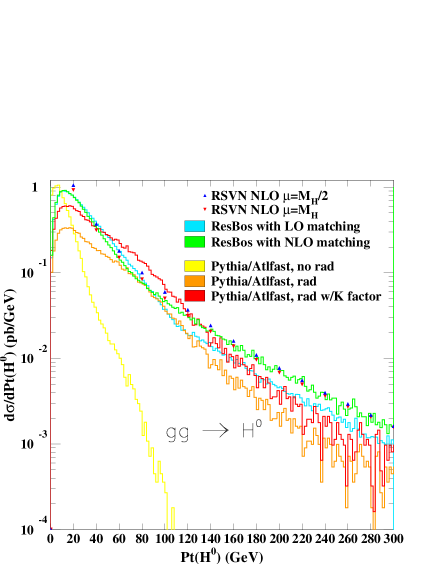
Figure 28: Transverse momentum distributions of 120 GeV Higgs bosons predicted by PYTHIA 6.210, ResBos, and the NLO calculation of Ravindran, Smith and Van-Neerven.

To realistically estimate the acceptance and other detector effects, we need predictions for NLO differential cross sections, especially for the transverse momentum ($P_{t}$) distribution of Higgs bosons. We computed these with ResBos, which calculates the total cross section and invariant mass distribution at NLO and the $P_{t}$ distribution shape at the resummed level with NLO matching and normalization [200, 202]. ResBos decays the Higgs boson to two photons, in a very good agreement with HDecay [165]. These photons are reconstructed after smearing the final states photon momenta according to the ATLAS detector performance [210, 211]. This distribution is compared to other predictions in Fig. 28.

The ResBos distribution, with NLO matching and renormalization and factorization scales $\mu_{R}=\mu_{F}=M_{H}$, shows a very good agreement with the recent NLO calculation [212] at the intermediate to high $P_{t}$. The deviation between the NLO matched ResBos (light green) histogram and the NLO prediction (red triangles) is in the order of the MC statistics, which is less than about 10% for $P_{t}\sim M_{H}$. In the low $P_{t}$, without initial and final state radiation, PYTHIA predicts a much softer spectrum than ResBos. But if we allowed for radiation in PYTHIA, we were not able to reproduce the shape of the $P_{t}$ distribution predicted by the other calculations. The ResBos total rate is found to be $\sigma=36.7$ pb, in excellent agreement with the HiGlu prediction of $\sigma=36.4$ pb.

12.3 The diphoton background

In this section we compare results of various calculations for the irreducible diphoton background of Higgs production. At the lowest order the most important contributors are the $q{\bar{q}}\to\gamma\gamma$ (Born) and the $gg\to\gamma\gamma$ (box) subprocesses. At the LHC, with CTEQ6L1, PYTHIA predicts 35.0 and 37.8 pb total cross sections, respectively. (Here $p_{t}>25$ GeV required for each photon.) Since PYTHIA yields a very soft $P_{t}$ distribution for the photon pair, we use two other MC codes to compute the diphoton $P_{t}$: Diphox and ResBos.

The Diphox code implements the NLO QCD calculation of the $q{\bar{q}}+{\bar{q}}^{(~{}\,)}g\to\gamma\gamma X$, and the LO calculation of the $gg\to\gamma\gamma$ subprocess. (These are referred to as direct processes). It also includes the single and double fragmentation processes as schematically depicted in Table 5(a). The NLO singularities, related to parton emission collinear to one of the photons, are regulated by a cone of radius $R$ around each photons. Since Diphox slices the phase space in the $P_{t}$ variable, its prediction for the $P_{t}$ distribution depends on non- physical parameters which handicaps its use in the experimental analysis.

ResBos implements a generalized factorization formalism applied to diphoton production [196, 197, 198]. As a result, it includes the direct processes up to NLO for the $q{\bar{q}}+{\bar{q}}^{(~{}\,)}g\to\gamma\gamma X$ and the $gg\to\gamma\gamma X$ subprocesses (except the two loop virtual corrections to the gluon fusion subprocess), and also the resummation of $\log(P_{t}/M_{\gamma\gamma})$ (where $M_{\gamma\gamma}$ is the mass of the photon pair). ResBos matches the resummed low $P_{t}$ prediction to the high $P_{t}$ NLO distribution [196]. This feature enables ResBos to give a correct prediction of the full $P_{t}$ distribution which is important at the Higgs search when a likelihood ratio method is used to reject background. Finally, ResBos implements fragmentation at LO.

The full NLO QCD corrections to the gluon fusion subprocess, including the two loop $gg\to\gamma\gamma$ virtual corrections were recently calculated [207]. The NLO K-factor $K_{NLO/LO}$ was found to be about 1.6 for an invariant mass of $M_{\gamma\gamma}=120$ GeV. The authors also demonstrated the reduction of the scale dependence in the NLO calculation.

	$80<M_{\gamma\gamma}<140$ GeV,      $p_{t_{\gamma}}\geq 25$ GeV,
	$|\eta|_{\gamma}<2.4$,      $R=0.4$,      ${E_{T}}_{cone}\leq 15$ GeV.
	(b) Cuts on the diphoton final state.
	Process	Contribution	Diphox	ResBos
	$q\bar{q}+{\bar{q}}^{(~{}\,)}g$	direct	$9.23$	$13.2$
	$\to\gamma\gamma$	total	$19.1$	$18.5$
	$gg\to\gamma\gamma$	direct	$5.47$	$6.85$

Table 5: (a) Schematic nomenclature used by Diphox for            (c) Diphoton  production  cross  sections,  in  picobarns,  at direct, one, and two fragmentation processes.                         the LHC with CTEQ6M and cuts given above.

Numerical results

In this section we present numerical results for the total cross section, the invariant mass ($M_{\gamma\gamma}$) and the transverse momentum ($P_{t}$) distributions of the diphoton system calculated by various codes. All these results are computed for the LHC ($pp$ collisions at $\sqrt{S}=14$ TeV) with CTEQ6M PDF (unless stated otherwise) and with equal renormalization and factorization scales $\mu_{F}=\mu_{R}=M_{\gamma\gamma}$. Since our interest is the background to a light Higgs boson, we limit all the events in the mass region $80<M_{\gamma\gamma}<140$ GeV. Besides, we request the standard ATLAS cuts given in Table 5(b). For $q{\bar{q}}+{\bar{q}}^{(~{}\,)}g\to\gamma\gamma X$ we use Diphox and ResBos while for $gg\to\gamma\gamma X$ we also show results of the NLO calculation by Bern, Dixon and Schmidt [214].

The total cross sections, obtained by Diphox and ResBos, are summarized in Table 5(c). ResBos tend to predict higher direct cross sections since in addition to the NLO contribution the infinite tower of $\alpha_{S}^{n}\log^{m}(P_{t}/M_{\gamma\gamma})$ is also included. On the other hand, Diphox implements NLO fragmentation while ResBos does this at LO. The higher ResBos rate is also due in part to the fact that the resummation calculation integrates over the soft radiation and thus provides no information about the soft partons around the photons. As a result, at low $P_{t}$, the ${E_{T}}_{cone}\leq 15$ GeV cut is not imposed on ResBos. In spite of the above listed differences, the total cross sections computed by the two codes agree within 4% after summed over all the final states. As Table 5(c) shows, at the LHC, the dominant contribution is coming from the $q{\bar{q}}+{\bar{q}}^{(~{}\,)}g$ initiated subprocesses. These subprocesses yield about 75-80% of the total rate.

Figure 29: Invariant mass and transverse momentum distributions for the $q\bar{q}+{\bar{q}}^{(~{}\,)}g\to\gamma\gamma$ subprocesses by Diphox and ResBos.

Fig. 29 shows the invariant mass and transverse momentum distributions for processes initiated by $q\bar{q}$ or ${\bar{q}}^{(~{}\,)}g$. Overall there is a good agreement between Diphox and ResBos in the relevant kinematic regions. The two codes somewhat disagree for low values of $M_{\gamma\gamma}$ but, fortunately, they agree for $M_{\gamma\gamma}>110$ GeV within the statistical uncertainties. The low and mid $P_{t}$ prediction of Diphox suffers from the problem of phase space separation and agreement with ResBos is not expected. On the other hand, according to expectations, in the high $P_{t}$ region the two predictions agree within the statistical errors.

In Fig. 30 the $M_{\gamma\gamma}$ and $P_{t}$ distributions are shown for the $gg\to\gamma\gamma X$ subprocess. Here we used CTEQ6L1 for the LO and CTEQ6M for the NLO distributions. For $M_{\gamma\gamma}$ the Diphox and the LO analytic calculation [214] are in agreement as expected. The ResBos rate is somewhat higher due to the additional logarithmic contributions which are enhanced for the $gg$ initial state. ResBos also overestimates the NLO results, which is probably due to the fact that the $gg\to\gamma\gamma$ two loop virtual corrections are missing from it. For low invariant masses PYTHIA tend to agree with ResBos while it favors the NLO result at larger $M_{\gamma\gamma}$. On the one hand, comparison of the LO and NLO QCD calculation emphasizes the importance of the implementation of the full NLO corrections in the MC codes. On the other, comparison of the LO QCD calculation and PYTHIA shows the importance of the initial state radiation. The almost 30% scatter of the various predictions shows that each of them is missing an important part of the known QCD corrections.

For the $P_{t}$ distribution, the Diphox prediction peaks at zero since this process is LO in Diphox. ResBos and PYTHIA provide soft gluon radiation so their spectra are broader. ResBos also contains the $gg\to\gamma\gamma g$ real emission contribution. On the other hand, as it was shown in Ref. [198], this contribution is almost negligible, so we do not include it here.

Figure 30: Distributions for the $gg\to\gamma\gamma X$ subprocesses predicted by Diphox, PYTHIA, ResBos and a NLO analytic calculation. The $P_{t}$ spread in the PYTHIA spectrum reflects the resolution of the ATLAS detector.

12.4 Summary

This work describes the present status of the diphoton cross section calculations at LHC. The total cross section, invariant mass and transverse momentum distributions have been compared using various codes. First, we considered the $pp(gg)\to H(\to\gamma\gamma)X$ process and compared predictions of PYTHIA and ResBos to a recent NLO calculation. We found an excellent agreement between ResBos and the NLO code in the mid to high $P_{t}$. Then, for the irreducible background, we computed both the $q{\bar{q}}+{\bar{q}}^{(~{}\,)}g\to\gamma\gamma X$ and the $gg\to\gamma\gamma X$ subprocesses. For $q{\bar{q}}+{\bar{q}}^{(~{}\,)}g\to\gamma\gamma X$ comparison of Diphox and ResBos showed encouraging agreement within the generated statistics. In case of the less explored gluon fusion subprocess ($gg\to\gamma\gamma X$), we found significant (${\mathcal{O}}$(30%)) differences between the MC and recent analytic QCD calculations. We believe that the implementation of the NLO gluon fusion process in the MC codes would benefit the Higgs search at the LHC. The impact of these results on the Higgs research will be analyzed in a separate work.

13 NLO corrections to $V+$jets

13.1 Introduction

The Higgs search is one of the highest priorities for the LHC physics program. While a plethora of phenomenological and detector studies have shown that the LHC has significant capability to discover a Higgs of any allowed mass in multiple channels, for many of those channels the background rates are known only at LO. This implies large uncertainties in how much luminosity it will take to detect a Higgs candidate in some channel, but more importantly it affects the more important task of measuring all the quantum properties of that candidate. We must improve our knowledge of the SM rates containing the same final states as the Higgs channels to as high a degree as possible, either by calculating quantum corrections to those processes, or establishing a reliable technique of measuring the SM rates in sidebands where we are confident there is no Higgs.

Our results here are improvements on the theoretical predictions. We have taken the previous results of NLO QCD corrections to $Wjj$ and $Zjj$ production [215, 216], where the jets may or may not be heavy flavor, and applied them to two cases of interest in the Higgs program: $Zjj$ production as a background to weak boson fusion (WBF) Higgs production, where the jets are very far forward/backward in the detector; and $Wb\bar{b}$ production, one of the principal backgrounds to $WH$ production in the $H\to b\bar{b}$ decay mode.

13.2 $Zjj$

The first channel, WBF Higgs production with subsequent decay to tau leptons [85, 86], $pp\to Hjj\to\tau^{+}\tau^{-}jj$, is also one of the most important. It is the only fermionic Higgs decay channel with both large rate and large signal to background ratio. Thus it is a crucial input necessary for extracting Higgs couplings. It is also a powerful channel in MSSM scenarios, providing a No-Lose Theorem for observing at least one of the CP-even states [217]. Finally, any of the WBF channels provide information on the gauge coupling strength and tensor structure of the Higgs to weak bosons, via the azimuthal angular distribution of the two “tagging” jets [218].

Because the Higgs is emitted with significant $p_{T}$ in this production mode, the taus will generally not lie back-to-back in the transverse plane, and their very nearly collinear decays allow for complete reconstruction, such that the Higgs resonance is visible with a width on the order of 10-15 GeV [219, 220]. The nearby $Z$ resonance in taus has a significant tail in the tau invariant mass distribution which overlaps the Higgs signal. We thus need a precise prediction for this contribution. QCD $Zjj$ production is several orders of magnitude larger than the signal, but it is greatly reduced in the phase space region populated by $W$-scattered forward quarks in WBF. Because of this, we require a separate NLO calculation in just this phase space region of high invariant mass, forward-scattered jets.

Our previous work [216] established the basic size of the NLO corrections in the WBF Higgs search region. For a fixed factorization and renormalization scale of the $Z$ mass, $\mu\equiv\mu_{f}=\mu_{r}=M_{Z}$, the corrections are about $15\%$ positive and have little residual combined scale dependence. At LO, a lower scale increases the cross section. All previous studies of this channel used lower scales, but implemented them dynamically, typically as the minimum or average $p_{T}$ of the tagging jets. As a dynamical scale is theoretical inconsistent at NLO, we cannot easily make comparison to the existing studies; they should be reperformed. However, we can surmise from the scale dependence that they overestimated the QCD $Zjj$ contribution by a modest amount.

Also important is the azimuthal angular distribution of the tagging jets. This distribution changes significantly at NLO, as shown in Fig. 31. Specifically, it flattens out considerably relative to the LO expectation. However, this does not take into account the minijet veto used in all WBF analyses: additional central jets of $p_{T}>20$ GeV cause the event to be vetoed, as these tend to appear only in QCD backgrounds and not the Higgs signal. Unfortunately, a veto for such a low $p_{T}$ range at NLO produces nonsense: the distrubution actually becomes negative for some angles. This is because of the delicate cancellations between the 2-jet virtual component and the soft singularities in the 3-jet real emission contribution, which cancel. Without a resummation calculation to correct the $p_{T}$ distrbution of the soft central jet, we cannot predict the tagging jet angular distribution at NLO with a minijet veto.

We can, however, subtract from the NLO distribution the LO $Zjjj$ distribution where the third jet satisfies the minijet veto criteria. The total rate $Zjjj$ is normalized to the NLO total rate via the truncated shower approximation [83], which approximates a NLO-resummed result. The result is that the rate is greatly reduced, as expected with the minijet veto, but the tagging jets’ azimuthal angular distribution remains mostly flat, closer to the NLO result than the LO result. This is a significant result, and currently state of the art, but clearly a full resummation calculation is highly desirable.

Figure 31: Azimuthal angular distribution of the tagging jets in QCD $Zjj$ production at LO (dashed) and NLO (solid) in the phase space region applicable to WBF Higgs searches. The gap between the two tagging jets is greater than 4 units of rapidity. The dotted curve is the NLO “vetoed” rate as explained in the text.

13.3 $Wb\bar{b}$

The second channel, $W$-associated production with subsequent decay to a pair of bottom quarks, $pp\to WH\to\ell\nu b\bar{b}$, is a weak channel statistically [221, 222], but highly desirable as it could give access to the $b$ Yukawa coupling.

The NLO QCD corrections to the background, QCD $Wb\bar{b}$ production, are surprisingly large, about a factor 2.4 [216] in the relevant phase space region of the Higgs resonance. We show the $b$-pair invariant mass distribution in Fig. 32. The large enhancement at NLO comes from additional Feynman diagrams that enter at NLO in the real emission, which are gluon-initiated; only quark-initiated processes exist at LO. The extra jet is typically hard and can be vetoed, but as in the $Zjj$ case this is unreliable at NLO. Therefore the NLO+veto curve in Fig. 32 has again a large uncertainty, which can be reduced only be performing a NLO calculation of the $Wb\bar{b}j$ rate. As a result, the impact of these corrections on the $WH;H\to b\bar{b}$ channel are uncertain, but not optimistic.

Figure 32: Bottom quark pair invariant mass distribution at LO (dashed) and NLO (solid), and with a veto on the additional light jet (dotted), for kinematic cuts corresponding to a Higgs search in $WH$ production.

14 Radiative Corrections to Di–Photon $+$ 1 Jet Production

14.1 Introduction

Higgs production in association with a jet of high transverse energy $E_{\rm T}$ with a subsequent decay into two photons, $pp\to H\ +{\rm jet}\to\gamma\gamma+{\rm jet}$, is considered a very promising discovery channel for a Higgs boson of intermediate mass (100 GeV $\mathrel{\raisebox{-2.58334pt}{$\stackrel{{\scriptstyle\textstyle<}}{{\sim}}$}}m_{\scriptscriptstyle H}\mathrel{\raisebox{-2.58334pt}{$\stackrel{{\scriptstyle\textstyle<}}{{\sim}}$}}$ 140 GeV) [223, 224]. In fact if a high-$p_{\rm T}$ jet is present in the final state, the photons are more energetic than in the inclusive channel and the reconstruction of the jet allows for a more precise determination of the interaction vertex. Moreover, the presence of the jet offers the advantage of being more flexible with respect to choosing suitable acceptance cuts to curb the background. These advantages compensate for the loss in the production rate. The analysis presented in Refs. [223, 224] was done at the parton level, for LHC operating at low luminosity (30 fb^-1 of accumulated data). It included only leading-order perturbative predictions for both the signal [225] and for the background [226], although anticipating large radiative corrections which were taken into account by using a constant $K^{\rm NLO}=1.6$ factor for both the signal and the background processes.

In the analysis of Refs. [223, 224], two photons with $p_{\gamma{\rm T}}\geq 40\mbox{~{}GeV}$ and $|\eta_{\gamma}|\leq 2.5$, and a jet with $E_{{\rm jet}{\rm T}}\geq 30\mbox{~{}GeV}$ and $|\eta_{\rm jet}|\leq 4.5$ were selected, with a photon-photon distance $\Delta R_{\gamma\gamma}\geq 0.3$ and a jet-photon distance $\Delta R_{\gamma{\rm jet}}\geq 0.3$. The binning of the photon-photon invariant mass $M_{\gamma\gamma}$ was taken to be $\Delta M_{\gamma\gamma}=3.25~{}(2.0)~{}\mbox{GeV}$ for ATLAS (CMS), with a photon identification efficiency of 73%. A cut over the parton centre-of-mass energy, $\sqrt{\hat{s}}\geq 300$ GeV, was used in order to improve the signal-over-background ratio, $S/B$. It was found that for a Higgs mass of $m_{\scriptscriptstyle H}=120$ GeV, the significance $S/\sqrt{B}$ was well above the discovery limit, both for the ATLAS and CMS detectors.

Using CompHEP [226] and PYTHIA [203, 227], the analysis of Refs. [223, 224] was repeated at the hadron level [228] for the ATLAS detector. The same cuts as in the analysis of Refs. [223, 224] were used, except for $\Delta R_{\gamma{\rm jet}}\geq 0.4$ and a different size in the binning of the photon-photon invariant mass $\Delta M_{\gamma\gamma}=3.64\mbox{GeV}$, with a photon identification efficiency of 80%. At the parton level, the analysis of Ref. [228] was consistent with Refs. [223, 224], and at the hadron level it found that the significance $S/\sqrt{B}$ was about at the discovery limit. In the analysis of Ref. [228], no $K$ factor was used either in the signal or in the background.

Since the first analyses of Refs. [223, 224] were made, the next-to-leading order (NLO) radiative corrections to the signal [39, 40, 41, 229] and to the background [230] have been computed. The main contribution to the signal comes from Higgs production via gluon fusion, where the interaction between the gluons and the Higgs is mediated by a loop of heavy quarks (in the Standard Model, with an accuracy of the order of 0.1%, one can limit oneself to consider only the top quark circulating in the loop). $H\ +{\rm jet}$ production via gluon fusion at leading order was evaluated in Ref. [225]. As regards the NLO contribution, only the bremsstrahlung corrections are known [231]. However, the full NLO corrections [39, 40, 41, 229] have been evaluated in the large $m_{\rm top}$ limit [232, 233], which for $H\ +{\rm jet}$ production is valid as long as $m_{\scriptscriptstyle H}\mathrel{\raisebox{-2.58334pt}{$\stackrel{{\scriptstyle\textstyle<}}{{\sim}}$}}2m_{\rm top}$ and the transverse energy is smaller than the top-quark mass $E_{\rm T}\mathrel{\raisebox{-2.58334pt}{$\stackrel{{\scriptstyle\textstyle<}}{{\sim}}$}}m_{\rm top}$ [234]. Furthermore, the large $m_{\rm top}$ limit is insensitive to the jet-Higgs invariant mass becoming larger than $m_{\rm top}$ [235]. For a Higgs mass of $m_{\scriptscriptstyle H}=120$ GeV, the NLO corrections were found to increase the leading-order prediction by about 60% [39, 40, 41, 229].

The NLO corrections to the background, $pp\to\gamma\gamma+{\rm jet}$, have been computed in Ref. [230], using the known NLO matrix elements [236, 237, 238]. The quark-loop mediated $gg\to g\gamma\gamma$ sub-process, which is ${\cal O}(\alpha_{\scriptscriptstyle S}^{3})$ and thus formally belongs to the NNLO corrections, and might have been significant due to the large gluon luminosity, had been computed previously and found to yield a modest contribution [239, 198]. In Ref. [230] the same cuts for photons and jets, $p_{\rm T}>40$ GeV and $|\eta|<2.5$, as in Ref. [239] were used. The midpoint cone algorithm [95] with a cone size of $R=\sqrt{\Delta\eta^{2}+\Delta\phi^{2}}=1$ was used in order to find the jet. Furthermore, both photons were isolated from the partons in a cone of size $R_{\gamma}=0.4$.

At NLO the isolated photon cross section is not infrared safe. To define an infrared safe cross section, one has to allow for some hadronic activity inside the photon isolation cone. In a parton level calculation it means that soft partons up to a predefined maximum energy are allowed inside the isolation cone. The standard way of defining an isolated prompt photon cross section, that matches the usual experimental definition, is to allow for transverse hadronic energy inside the isolation cone up to $E_{{\rm T},{\rm max}}$, where $E_{{\rm T},{\rm max}}$ is either a fixed energy value or it is equal to $\varepsilon p_{\gamma{\rm T}}$, with typical values of $\varepsilon$ between 0.1 and 0.5, and where $p_{\gamma{\rm T}}$ is taken either to be the photon transverse momentum on an event-by-event basis or to correspond to the minimum value in the $p_{\gamma{\rm T}}$ range. In perturbation theory this isolation requires the splitting of the cross section into a direct and a fragmentation contribution.

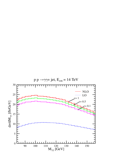
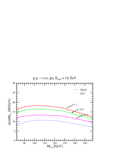
Figure 33: Dependence of the invariant mass distribution of the photon pair on the photon isolation parameter $\epsilon$ for $R_{\gamma}=0.4~{}(1.0)$ on the left(right)-hand-side panel. The photons and the jet are required to have transverse momentum $|p_{\rm T}|\geq 40$ GeV and lie in the central rapidity region of $|\eta|\leq 2.5$. In addition, it is required that $\Delta R_{\gamma{\rm jet}}\geq 1.5$ and $p_{\gamma\gamma,{\rm T}}\geq 40$ GeV. The dashed curve is the leading order prediction. The solid curves are the NLO corrections.

In Ref. [230], only the direct contribution to the production of two photons was included. That was possible thanks to a “smooth” photon-isolation prescription which does not require a fragmentation contribution [240]. This isolation prescribes that the energy of the soft parton inside the isolation cone has to converge to zero smoothly if the distance in the $\eta-\phi$ plane between the photon and the parton vanishes. Explicitly, the amount of hadronic transverse energy $E_{\rm T}$ (which in a NLO partonic computation is equal to the transverse momentum of the possible single parton in the isolation cone) in all cones of radius $r<R_{\gamma}$ must be less than

$$E_{{\rm T},{\rm max}}=\varepsilon p_{\gamma{\rm T}}\left(\frac{1-\cos r}{1-\cos R_{\gamma}}\right)^{n}\>,$$ (35)

In Ref. [230], $n=1$ and $\varepsilon=0.5$ were used as default values, and $p_{\gamma{\rm T}}$ was taken to be the photon transverse momentum on an event-by-event basis.

In Fig. 33, the distribution of the invariant mass $M_{\gamma\gamma}$ of the photon pair is analysed as a function of the photon isolation parameter $\epsilon$, for $R_{\gamma}=0.4$ and 1. Firstly, we note that the smaller $R_{\gamma}$ the larger the NLO correction. In fact, for $R_{\gamma}=0.4$ the $K$-factor is typically above 2. In addition, the larger $\epsilon$ the larger the NLO correction, with the effect being larger if $R_{\gamma}$ is larger. Another remarkable feature of Fig. 33 is that with the applied cuts, the two-photon plus jet background for the search of a Higgs boson with mass in the 120–140 GeV range is rather flat, therefore, well measurable from the sidebands around the hypothetical Higgs signal. This feature is very different from the shape of the background to the inclusive $pp\to H\to\gamma\gamma$ channel, which is steeply falling.

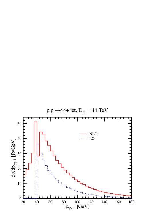
Figure 34: Transverse momentum distribution of the photon pair. The same selection cuts are used as in Fig. 1, with $R_{\gamma}=0.4$ and $\epsilon=0.5$.

In Fig. 34, we plot the differential distribution of the transverse momentum of the photon pair, $p_{\gamma\gamma{\rm T}}=|{\mbox{\boldmath$p$}}_{\gamma_{1},{\rm T}}+{\mbox{\boldmath$p$}}_{\gamma_{2},{\rm T}}|$, with a cut at $p_{{\rm jet}{\rm T}}^{\rm min}=40$ GeV. In accordance with the current experimental analyses, the photon isolation radius was taken to be $R_{\gamma}=0.4$. At leading order the jet recoils against the photon pair and the respective jet and photon pair $p_{\rm T}$ distributions are identical. At NLO the extra parton radiation opens the part of the phase space with $p_{\gamma\gamma{\rm T}}<p_{{\rm jet}{\rm T}}^{\rm min}$. The double peak around 40 GeV is an artifact of the fixed-order computation, similar to the NLO prediction at $C=0.75$ for the $C$-parameter distribution in electron-positron annihilation. The fixed-order calculation is known to be unreliable in the vicinity of the threshold, where an all-order resummation is necessary [241]. That would result in a structure, called Sudakov shoulder, which is continuous and smooth at $p_{\gamma\gamma{\rm T}}=p_{{\rm jet}{\rm T}}^{\rm min}$. Without the resummation, we must introduce a cut, $p_{\gamma\gamma,{\rm T}}\geq 40$ GeV to avoid regions in the phase space where the fixed-order prediction is not reliable. Accordingly, in Fig. 1 we have required that $p_{\gamma\gamma,{\rm T}}\geq 40$ GeV.

One of the goals of computing the radiative corrections to a production rate is to examine the behaviour of the cross section under variations of the renormalization $\mu_{\scriptscriptstyle R}$ and factorization $\mu_{\scriptscriptstyle F}$ scales. The analysis of Ref. [230] showed that the dependence of the cross section under variations of $\mu_{\scriptscriptstyle R}$ and/or $\mu_{\scriptscriptstyle F}$ remains about the same (in relative size) in going from the leading order to the NLO prediction, if the default value of the radius $R_{\gamma}=0.4$ (with $\epsilon=0.5$) is used, while it slightly decreases if the photon isolation parameters are taken to be $R_{\gamma}=1$ and $\epsilon=0.1$.

In conclusion, the analysis of Ref. [230] found large radiative corrections, however these are strongly dependent on the selection cuts and the photon isolation parameters. Choosing a small isolation cone radius $R_{\gamma}=0.4$ (which is nowadays the experimental preferred choice), with relatively large hadronic activity allowed in the cone, results in more than 100 % correction with a residual scale dependence which is larger at NLO than at leading order. Increasing the cone radius to $R_{\gamma}=1$ and decreasing the hadronic activity in the cone reduces both the magnitude of the radiative corrections as well as the dependence on the renormalization and factorization scales. This result shows that a constant $K^{\rm NLO}=1.6$ factor, as used in Refs. [223, 224], is certainly not appropriate for taking into account the radiative corrections to the irreducible background of the $pp\to H+{\rm jet}\to\gamma\gamma+{\rm jet}$ discovery channel at the LHC.

15 Top background extrapolation for $H\to WW$ searches

15.1 Introduction

Recent studies indicate that the LHC will be able to discover a Standard Model (SM) Higgs boson with mass between 100 and 200 GeV with an integrated luminosity of only 10 to 30 fb^-1 if weak boson fusion (WBF) followed by $H\to\tau\tau$ and $H\to WW$ channels are taken into account (see Ref. [242] and refs. therein). This intermediate mass range is currently favored in light of a lower bound of 114.1 GeV from direct searches at LEP2 and an upper bound of 196 GeV from a SM analysis of electroweak precision data (at 95% CL) [243, 244]. As discussed in detail in Ref. [62], Sec. A.1, the precise knowledge of the significance of any observed Higgs signal will require an accurate determination of the SM backgrounds. The WBF and gluon fusion $H\to WW\to llp\hskip-5.03125pt\hbox to5.03125pt{\hss$/$\hss}_{T}$ channels are particularly challenging, because missing momentum prevents the observation of a narrow mass peak that would allow an interpolation of the backgrounds from side bands.

In this section we demonstrate how the extrapolation approach proposed in Ref. [62] can in fact be used to reduce the uncertainty of the dominant $t\bar{t}$ + 1 jet background to the $H\to W^{+}W^{-}\to l_{1}^{\pm}l_{2}^{\mp}p\hskip-5.03125pt\hbox to5.03125pt{\hss$/$\hss}_{T}$ search in WBF and the large $t\bar{t}$ background to the same Higgs decay mode in gluon fusion. To be specific, we consider the $t\bar{t}j$ background in the WBF selection cuts of Ref. [110] and the $t\bar{t}$ background in the selection cuts suggested for the inclusive $H\to WW$ search in Ref. [59], Sec. 19.2.6, with a transverse mass window cut based on a Higgs mass of 170 GeV. All cross sections are calculated using the parton-level Monte Carlo programs of Refs. [245] and [246], which include finite width effects and the complete leading order (LO) matrix elements for $l_{1}^{\pm}l_{2}^{\mp}\nu\bar{\nu}b\bar{b}$ (+ jets) final states. The calculations take into account finite resolution effects and a suboptimal $b$ tagging efficiency based on expectations for the ATLAS detector.

To investigate the scale uncertainty of these backgrounds and how it can be reduced we apply the following definitions for the renormalization and factorization scales $\mu_{R}$ and $\mu_{F}$. A factor $\xi=\mu/\mu_{0}$ is then used to vary the scales around the central values. The suggestive scale choice for top production is the top mass $m_{t}=175$ GeV:

$$\mu_{R}=\mu_{F}=\xi m_{t}\,.$$ (36)

Results for this scale choice are shown as solid curves in Figs. 35 and 36. For WBF, due to forward tagging selection cuts, the dominant background arises from $t\bar{t}$ production with one additional hard jet. To avoid double counting in this case, we alternatively calculate with scales based on the minimal transverse mass:

$$\mu_{F}=\xi\min(m_{T,t},m_{T,\bar{t}},p_{T,j})\quad\text{and}\quad\alpha_{s}^{3}=\alpha_{s}(\xi m_{T,t})\alpha_{s}(\xi m_{T,\bar{t}})\alpha_{s}(\xi p_{T,j})\,.$$ (37)

Results for this second definition are shown as dashed curves in Fig. 35. In principle, the renormalization and factorization scales are independent. We find, however, that the strongest scale variation occurs if both scales are varied in the same direction and thus only introduce a single parameter $\xi$. Scale-dependent quantities are customarily condensed into the form $\hat{x}\pm\Delta\hat{x}$ based on a particular low and high scale choice. We use the convention

$$\hat{x}=(x(\xi=\frac{1}{2})+x(\xi=2))/2\quad\text{and}\quad\Delta\hat{x}=|x(\xi=\frac{1}{2})-x(\xi=2)|/2\;,$$ (38)

where $x$ is a cross section or cross section ratio.

Figs. 35(a) and 36(a) show the large scale variation that is expected for the LO background cross sections in both search channels. For the WBF search channel, the scale scheme of Eq. (36) yields a background cross section of $0.27\pm 0.11$ fb, whereas the scheme of Eq. (37) yields $0.41\pm 0.17$ fb. The theoretical uncertainty is about 40% in both cases. Since the second cross section is not consistent with the first within 1$\sigma$, it seems more appropriate to apply the prescription Eq. (38) to the envelope of both curves. All subsequent WBF results will be given using this procedure. Here, one obtains $0.38\pm 0.21$ fb, with an even larger uncertainty of 55%. For the top background in the inclusive $H\to WW$ search a somewhat smaller theoretical uncertainty is obtained, i.e. 3.7 fb with an uncertainty of 25%. In both cases it is obvious that the accuracy of theoretical background calculations at LO is insufficient to determine the total background to an accuracy of 10%, as assumed in Ref. [242].

15.2 Extrapolation

The extrapolation approach allows a more accurate determination of a background cross section $\sigma_{bkg}$ if a reference selection with a corresponding well-defined, measurable event rate $\sigma_{ref}\cdot{\cal L}$ can be found, so that the theoretical uncertainty of the ratio $\sigma_{bkg}/\sigma_{ref}$ is small and $\sigma_{ref}$ can be measured with low experimental uncertainty. The background cross section can then be approximated through

$$\sigma_{bkg}\quad\approx\quad\underbrace{\left(\frac{\sigma_{bkg,\text{ LO}}}{\sigma_{ref,\text{ LO}}}\right)}_{\stackrel{{\scriptstyle\mbox{\footnotesize low theoret.}}}{{\mbox{\footnotesize uncertainty}}}}\quad\cdot\quad\underbrace{\sigma_{ref}}_{\stackrel{{\scriptstyle\mbox{\footnotesize low experim.}}}{{\mbox{\footnotesize uncertainty}}}}\;.$$ (39)

To derive suitable reference selections from the corresponding background selections, we propose the following strategy: The WBF and inclusive $H\to WW$ search channel top backgrounds are effectively suppressed through a central jet veto. Discarding this veto leads to a sizable increase of the cross sections. Secondly, to identify the top backgrounds in both cases, we require that only events be considered that contain one or more identified $b$ jets. For our calculations we assume that $b$ jets with $|\eta|<2.5$ and $p_{T}>15$ GeV will be tagged with a probability of 60%. Finally, if the resulting reference rate is still too small, the lepton pair cuts are also discarded. This is only necessary in the WBF channel, where the reference cross section with lepton pair cuts is 10.8 fb, which, with 30 fb^-1, would result in a statistical uncertainty for the measured rate of about 6%.

Figure 35: Renormalization and factorization scale variation of $t\bar{t}j$ background cross section (a) and ratio with reference cross section (b) to $H\to W^{+}W^{-}\to l_{1}^{\pm}l_{2}^{\mp}p\hskip-5.03125pt\hbox to5.03125pt{\hss$/$\hss}_{T}$ search in weak boson fusion at the LHC for different scale definitions (see main text).

Consequently, the reference selection cuts for the WBF channel are obtained by imposing the identified $b$ jet requirement and discarding the veto of Eq. (4) and the lepton pair cuts of Eqs. (5, 6, 8, 9) in Ref. [110]. The resulting reference cross section of $96\pm 50$ fb gives rise to a statistical error of about 2% with 30 fb^-1 of data. Note that the scale uncertainty of this reference cross sections is very similar to that of the background cross section. However, the scale variation of the corresponding ratio $\sigma_{bkg}/\sigma_{ref}$ is significantly reduced as shown in Fig. 35(b). One obtains $0.0038\pm 0.0002$, or a relative error of 5%. Combining both extrapolation factors in quadrature yields a background estimate with an accuracy of about 5%.

Figure 36: Renormalization and factorization scale variation of $t\bar{t}$ background cross section (a) and ratio with reference cross section (b) to $H\to W^{+}W^{-}\to l_{1}^{\pm}l_{2}^{\mp}p\hskip-5.03125pt\hbox to5.03125pt{\hss$/$\hss}_{T}$ search in gluon fusion at the LHC.

For the $H\to WW$ in gluon fusion channel, suitable reference selection cuts are obtained by requiring at least one identified $b$ jet and applying the cuts on pp. 705-706 of Ref. [59], but without vetoing jets with $p_{T}<15$ GeV and $|\eta|<3.2$. Here, a reference cross section of $450\pm 88$ fb results, which is large enough that the lepton pair cuts can be kept. With 30 fb^-1 of data, the reference rate could be determined with a statistical accuracy of better than 1%. The scale variation of the ratio $\sigma_{bkg}/\sigma_{ref}$ is shown in Fig. 36(b). It is again significantly reduced. One obtains $0.0081\pm 0.0001$, or a relative error of 1%. Combining both extrapolation factors yields a background estimate with an accuracy of about 1% in this case.

15.3 Discussion

The approximation Eq. (39) would become an identity if the ratio $\sigma_{bkg}/\sigma_{ref}$ could be evaluated to all orders in perturbation theory. At fixed order in perturbation theory, a scale dependence remains and, depending on the specific scale choice, the result will deviate to a greater or lesser extent from the exact result. We refer to this error as residual theoretical error. In practice, it is commonly estimated from the scale variation using a prescription like Eq. (38). Since the scale variation typically decreases for higher fixed order calculations, it would be instructive to calculate $\sigma_{bkg}/\sigma_{ref}$ at NLO. We expect the NLO ratios and residual theoretical error estimates to be comparable to the ones obtained here, but this should be confirmed through explicit calculation. We further note that a future study could take into account systematic experimental uncertainties and parton distribution function uncertainties, once these become available.

15.4 Conclusions

A LO analysis was presented that demonstrates that key top backgrounds to $H\to W^{+}W^{-}\to l_{1}^{\pm}l_{2}^{\mp}p\hskip-5.03125pt\hbox to5.03125pt{\hss$/$\hss}_{T}$ decays in weak boson fusion and gluon fusion at the LHC can be extrapolated from experimental data with an accuracy of ${\cal O}(5\%)$. If LO scale variation is accepted as proxy for the theoretical error, our parton-level results indicate that the $t\bar{t}j$ background to the $H\to WW$ search in WBF can be determined with a total error of about 5%, while the $t\bar{t}$ background to the $H\to WW$ search in gluon fusion can be determined with a total error of about 1% with an integrated luminosity of 30 fb^-1. Further details can be found in Ref. [247].

16 Scale Dependence of $t\bar{t}b\bar{b}$ Production

The process $pp\rightarrow t\bar{t}b\bar{b}$ is the most important background to Higgs production in association with $t\bar{t}$ at the LHC [248]. The cross section of $t\bar{t}b\bar{b}$ production has been calculated with CompHEP [249] and ALPGEN [250] at leading order. Higher order corrections for $t\bar{t}b\bar{b}$ are unknown so far. In order to estimate the theoretical uncertainties, we vary the $Q^{2}$ scale.

In ALPGEN, the default scale choice is $Q^{2}=m_{t}^{2}$. Because we are mainly interested in $t\bar{t}b\bar{b}$ events in the phase space region which is accessible experimentally, we apply following cuts before the computation of the cross section or the event generation, respectively: $p_{T}(b)>$ 25 $GeV$, $|\eta(b)|<$ 2.4, and $\Delta R(b,b)>$ 0.4.

Fig. 37 shows the cross section as a function of the prescaling factor $\xi$. In the range between 0.5 and 2.0, the cross section changes by more than a factor of two. However, the invariant mass distributions of the two $b$-quarks, not coming from a top decay, seem to be not affected. Nevertheless, one should keep in mind, that the understanding of this mass distribution is experimentally the most relevant for the search of a Higgs mass peak on top of the background in the $t\bar{t}h$ channel. Additional jets from higher order contributions complicate the jet reconstruction and can increase the combinatorial background which has a different shape.

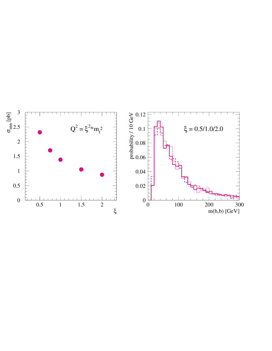
Figure 37: Left: $t\bar{t}b\bar{b}$ cross section as a function of the $Q^{2}$ scale prescaling factor $\xi$. Right: $b\bar{b}$ invariant mass distributions of the $b$-quarks not coming from top decays for three scale choices. All distributions are normalized to unit area. The cross sections and the mass distributions are obtained after following acceptance cuts: $p_{T}(b)>$ 25 $GeV$, $|\eta(b)|<$ 2.4, and $\Delta R(b,b)>$ 0.4.

17 Studying the Higgs sector at the LHC using proton tagging

17.1 Introduction

If the Higgs mechanism is responsible for the Electroweak Symmetry breaking in Nature, generally at least one Higgs boson should be discovered at the LHC. In particular, if the light Higgs predicted by the Standard Model (SM) exists it will almost certainly be found at the LHC in the first years of running, but detailed studies may be challenging, see [251] and references therein. However, beyond the SM, various extended models predict a large diversity of Higgs-like states with different masses, couplings and even $CP$-parities. In these models the properties of the neutral Higgs bosons can differ drastically from SM one. The most elaborated extension is the Minimal Supersymmetric Standard Model (MSSM), for a recent review see [252]. Below we shall mainly follow this benchmark model. The extended scenarios would complicate the study of the Higgs sector using the conventional (semi)inclusive strategies.

After the discovery of a Higgs candidate the immediate task will be to establish its quantum numbers, to verify the Higgs interpretation of the signal, and to make precision measurements of its properties. The separation of different Higgs-like states will be especially challenging. It will be an even more delicate goal to probe the $CP$ -parity and to establish the nature of the newly-discovered heavy resonance state(s).

As was shown in [253, 254], the central exclusive diffractive processes (CEDP) at the LHC can play a crucial role in solving these vital problems. These processes are of the form

$$pp\to p+\phi+p,$$ (40)

where the $+$ signs denote the rapidity gaps on either side of the Higgs-like state $\phi$. They have unique advantages as compared to the traditional non-diffractive approaches [255, 251]. In particular, if the forward protons are tagged, then the mass of the produced central system $\phi$ can be measured to high accuracy by the missing mass method. Indeed, by observing the forward protons, as well as the $\phi\to{b\bar{b}}$ pairs in the central detector, one can match two simultaneous measurements of the $\phi$ mass: $m_{\phi}=m_{\rm missing}$ and $m_{\phi}=m_{b\bar{b}}$. Thus, the prospects of the precise mass determination of the Higgs-like states, and even of the direct measurements of their widths and $\phi\to{b\bar{b}}$ couplings, look feasible. Another unique feature of the forward CEDP is that in the production vertex the incoming gluon polarisations are correlated, in such a way that the effective luminosity satisfies the P-even, $J_{z}=0$ selection rule [256, 255]. This plays a key role in reducing the QCD background caused by the $gg\to{b\bar{b}}$ subprocess. On the other hand, this selection rule opens a promising way of using the forward proton taggers as a spin-($CP$)parity analyser [253].

The cross section for the production of a CEDP SM Higgs at the LHC, with $m_{h}=120$ GeV is calculated [254] to be 2.2 fb with an uncertainty given by the range 0.9–5.5 fb. The inclusive diffractive process $pp\to p+\phi X+p$ has a larger cross section[257, 258, 259, 260] of order 100 fb, but there is no $J_{z}=0$ selection rule for the background and the Higgs mass cannot be determined directly from the scattered protons. Recently also the single diffractive channel was revisited and studied [261] (see also [262]), which has a much larger cross section.

Our main goal here is to show that forward proton tagging may significantly enlarge the potential of studying the Higgs sector at the LHC.

17.2 Potential of diffractive processes for Higgs studies

Over the last years such processes with rapidity gaps have attracted much attention as a promising way to search for a Higgs boson in high energy proton-proton collisions, see, for instance,  [263, 264, 265, 266, 255, 260, 257, 258, 267, 253, 268].

The CEDP have special advantages in the regions of the MSSM parameter space where the partial width of the Higgs boson decay into two gluons much exceeds the SM case. First of all ,this concerns the large $\tan\beta$ case,where the expected CEDP cross sections are large enough,see [254]. Of special interest is the so-called “intense-coupling” regime [405], where the masses of all three neutral Higgs bosons are close to each other. Here the $\gamma\gamma,WW^{\star},ZZ^{\star}$ decay modes (which are among the main detection modes for the SM Higgs) are strongly suppressed. This is the regime where the variations of all MSSM Higgs masses and couplings are very rapid. This region is considered as one of the most troublesome for the (conventional) Higgs searches at the LHC, see [405]. On the other hand, here the CEDP cross sections are enhanced by more than an order of magnitude. Therefore the expected significance of the CEDP signal becomes quite large. Indeed, this is evident from Fig. 1, which shows the cross sections for the CEDP production of $h,H,A$ bosons as functions of their mass for $\tan\beta=30$ and 50.

Figure 38: The cross sections, times the appropriate ${b\bar{b}}$ and $\tau^{+}\tau^{-}$ branching fractions, predicted (see [254])for production of $h(0^{+})$, $H(0^{+})$ and $A(0^{-})$ MSSM Higgs bosons at the LHC. The dotted curve in the upper plots shows the cross section for a SM Higgs boson.

Let us focus on the main $\phi\to{b\bar{b}}$ decay mode.

The estimates of the event rates in Ref. [251] were performed assuming $\sigma_{\rm CEDP}$=3 fb, a proton tagging efficiency of 0.6 and a $b$ jet tagging efficiency of 0.6. Furthermore the signal has been multiplied by 0.5 to account for the jet polar angle cut and by 0.67 for the $b\bar{b}$ branching fraction. It is expected  [251] that proton taggers can achieve a missing mass resolution of $\Delta m_{\rm missing}\simeq 1$ GeV, giving a background of 4 events for an integrated luminosity of ${\cal L}=30~{}{\rm fb}^{-1}$. For such a luminosity, taking into account the efficiencies, we would expect a Higgs signal of 11 events with a favourable signal-to-background ratio $S/B\sim 3$. Thus, to obtain a statistical significance of $5\sigma$ it is sufficient for the cross section for a ${b\bar{b}}$ signal to satisfy

$${\rm Br}({b\bar{b}})\cdot\sigma>0.7~{}{\rm fb}~{}(2.7~{}{\rm fb})$$ (41)

for an integrated luminosity to be ${\cal L}=300~{}{\rm fb}^{-1}$ (30 fb^-1).

In the MSSM case, as can be seen from Fig. 1, at $\tan\beta=50$ we expect that ${\rm Br}(H\to{b\bar{b}})\sigma_{H}$, is greater than 0.7fb for masses up to $m_{H}\sim 250$ GeV. The situation is worse for pseudoscalar, $A$, production, because of the $P$-even selection rule. Thus, the CEDP filters out pseudoscalar production, which allows the possibility to study pure $H$ production, see Fig. 1. This may be also useful in the decoupling limit ($m_{A}>2m_{Z}$ and $\tan\beta>5$), where the light scalar $h$ becomes indistinguishable from the SM Higgs, and the other two neutral Higgs states are approximately degenerate in mass. Here, forward proton tagging can play an important role in searching for (at least) the $H$-boson, if it is not too heavy ($m_{H}{\;\raisebox{-3.01385pt}{$\stackrel{{\scriptstyle\textstyle<}}{{\sim}}$}\;}250$ GeV). For large values of $\tan\beta$ the decoupling regime essentially starts at $m_{A}\simeq 170$ GeV. As seen in Fig. 1, the cross section is still sufficiently large to ensure the observation of the $H$ boson up to $m_{A}\simeq 250$ GeV. The possibility to use diffractive processes to explore larger masses will depend on various experiment-related factors. In particular, on the prospects to achieve better mass resolution, $\Delta m$, at higher mass, $m$. As discussed in Ref. [254], CEDP may cover also the regions of MSSM parameter space (‘window’ or ‘hole’ regions,see for example, [252] ) where, once the $h$ boson is discovered, it is not possible to identify the $H$ scalar by traditional means at the $5\sigma$ confidence even with 300 fb^-1 of combined ATLAS+CMS luminosity.

As mentioned above, if a candidate signal is detected it will be a challenging task to prove its Higgs identity. Unlike the conventional approaches, the very fact of seeing the new state in CEDP automatically implies that it has the following fundamental properties. It must have zero electric charge and be a colour singlet. Furthermore, assuming $P$ and $C$ conservation, the dominantly produced state has a positive natural parity, $P=(-1)^{J}$ and even $CP$. The installation of forward proton taggers may provide valuable additional leverage in establishing the origin of the newly discovered candidate state. In particular, assuming CP conservation, the CEDP allow the $0^{-},1^{-},1^{+}$ states to be filtered out, leaving only an ambiguity between the $0^{++}$ and $2^{++}$ states. Though without further efforts the $2^{++}$ state cannot be ruled out, this would not be the most likely choice.

Figure 39: The mass bands $m_{\phi}\pm\Gamma$ for neutral MSSM Higgs bosons as a function of $m_{A}$. The upper right hand plot shows that the $h$ and $H$ bosons are clearly identifiable for $\tan\beta=30$, if $A(0^{-})$ production is suppressed. The lower plots show how the sensitivity of the widths, to variations of $\tan\beta$, will change the profile of the peaks.

As discussed in [253, 269], studying of the azimuthal correlations of the outgoing protons can allow further spin-parity analysis. In particular, it may be possible to isolate the $0^{-}$ state. particles [253]. Note that with the forward protons we can determine the $CP$-properties of the Higgs boson irrespective of the decay mode. Moreover, CEDP allow the observation of the interference effects between the CP-even and CP-odd $gg\to\phi$ transitions. Their observation would signal an explicit $CP$-violating mixing in the Higgs sector.

To illustrate how the CEDP can help to explore the Higgs sector let us consider again large $\tan\beta$ case. In the intense coupling regime it is especially difficult to disentangle the Higgs bosons in the region around $m_{A}\sim 130$ GeV, where there is almost a mass degeneracy of all three neutral Higgs states and their total widths can be quite large and reach up to 1–2 GeV. This can be seen from Fig. 2, where for numerical purposes, the same parameters as in [405] were chosen. Since the traditional non-diffractive approaches do not, with the exception of the $\gamma\gamma$ and $\mu\mu$ modes, provide a mass resolution better than 10–20 GeV, all three Higgs bosons will appear as one resonance. Recall that in this regime the $\gamma\gamma$ decay mode is hopeless and the dimuon Higgs decay mode is quite rare (and, anyway, would require that the Higgs mass splitting exceeds at 3–5 GeV, see Ref. [405]). An immediate advantage of CEDP, for studying this region, is that the $A$ contribution is strongly suppressed, while the $h$ and $H$ states can be well separated ($m_{H}-m_{h}\simeq 10$ GeV) given the anticipated experimental mass resolution of $\Delta M\sim 1$ GeV [251], see Fig. 2. Note,that the forward tagging approach can provide a direct measurement of the width of the $h$ (for $m_{h}{\;\raisebox{-3.01385pt}{$\stackrel{{\scriptstyle\textstyle<}}{{\sim}}$}\;}120$ GeV) and the $H$-boson (for $m_{H}{\;\raisebox{-3.01385pt}{$\stackrel{{\scriptstyle\textstyle>}}{{\sim}}$}\;}130$ GeV). Outside the narrow range $m_{A}=130\pm 5$ GeV, the widths of the $h$ and $H$ are quite different (one is always much narrower than the other). It would be instructive to observe this phenomenon experimentally.

For $\tan\beta=30$ the central exclusive signal should be still accessible at the LHC up to an $H$ mass about 250 GeV. For instance, for $m_{H}=210$ GeV, and LHC luminosity $30~{}{\rm fb}^{-1}$ ($300~{}{\rm fb}^{-1}$), about 20 (200) $H\to{b\bar{b}}$ events are produced. If the experimental cuts and efficiencies quoted in [251] are imposed, then the signal is depleted by about a factor of 6. This leaves 3 (30) observable events, with background of about 0.1 (1) events.

Let us make a few comments about the possibility to identify the pseudoscalar boson, $A$, see for detailes Ref. [253, 254]. If the CEDP cross sections for scalar and pseudoscalar Higgs production were comparable, it would be possible to separate them readily by the missing mass scan, and by the study of the azimuthal correlations between the proton momenta. However,the cross section for pseudoscalar Higgs exclusive production is strongly suppressed.For values of $\tan\beta\sim 10$–15, the separation between the $H/h$ and $A$ bosons is much larger than their widths, see Fig. 2 . Hence it might be just possible to observe the pseudoscalar in CEDP. For example, for $\tan\beta=15$ and $m_{A}=95$ GeV, the mass separation, 3.6 GeV, between $h$ and $A$ is about 8 times larger than the width $\Gamma_{h}$. The cross section

$${\rm Br}(A\to{b\bar{b}})\cdot\sigma_{A}\simeq 0.15~{}{\rm fb},$$ (42)

when allowing for the large uncertainties in $\sigma_{A}$, could be just sufficient to bring the process to the edge of observability.

Probably the best chance to identify the $A(0^{-})$ boson is to observe the double-diffractive inclusive process

$$pp\to X+\phi+Y,$$ (43)

where both protons are destroyed. Process (43) has the advantage of a much larger cross section, see Ref. [255]. However,here we do not have the $J_{z}=0$ selection rule to suppress the $b\bar{b}$ background, nor do we have the possibility of the good missing mass resolution. On the other hand, the $gg^{PP}$ luminosity is more than order of magnitude larger than for the pure exclusive case. For example, for double-diffractive inclusive production, with the rapidity gaps $\Delta\eta>3$, the luminosity is 20 times larger than that for the exclusive diffractive production of a Higgs boson with mass $m_{H}=120$ GeV. So, even for the $\tau\tau$ decay mode we expect a cross section, $\sigma_{\rm incl}$, of about 20 fb for $A$ production in the MSSM with $\tan\beta=30$ and $m_{A}=120$ GeV. This looks promising, provided that the probability for gluon misidentification as a $\tau$ is less than 1/150, which looks feasible. Process (43) may be also useful in searches for a light $CP$-violating Higgs boson, where we can study, azimuthal correlations between the outgoing transverse energy flows of the dissociating systems, see Ref. [269].

17.3 Experimental challenges

The centrally produced Higgs particles can be measured with the ATLAS and CMS general purpose detectors at the LHC. In order to tag the scattered protons these experiments will need to be equipped with detectors that need to be integrated with the beamline of the LHC. Due to the relatively low mass of the central (Higgs) system, the scattered protons have small $\xi$ values, in the range of $10^{-3}$–$10^{-2}$, where $\xi$ is the momentum fraction lost by the proton in the interaction. A classical technique to detect scattered protons at small $t$ and with small relative momentum loss, is by using so-called roman pot detectors. Recently a new type of detectors, called microstations [270], has been proposed for this purpose. Studies of the LHC beam optics [271] reveal that, in order to access these small $\xi$ values, the roman pot detectors or microstations need to be installed at about 300 m from the interaction region. These detectors can have an acceptance in $\xi$ down to 1–2$\times 10^{-3}$, and a parametrization of the acceptance was included in the event estimates given before.

In order to efficiently record and measure the diffractively scattered protons in roman pot detectors or microstations, they have to be sufficiently separated from the beam particles. The detectors, which are located at 330 m and 420 m from the interaction point, could then be used to define the proton momenta by measuring, with respect to the beam axis, the difference in horizontal displacement at the two locations as a function of the average proton deflection.

We observe that a variation of $\Delta\xi=5\times 10^{-4}$ produces a $80\>\mu{\rm m}$ difference in the horizontal displacement of a diffractively scattered proton. With state-of-the-art silicon microstrip detectors this difference can be measured with a precision of the order of 5$\mu$m. The expected momentum spread of the beam protons is $\Delta\xi/\xi=10^{-4}$. For a symmetric event configuration ($\Delta=|\xi_{1}-\xi_{2}|\leq 0.04$), we then expect in the most optimistic case a mass resolution of the order of $\Delta M_{\rm missing}/M_{\rm missing}$ of order of 1% [271].

Pile-up events will also be important for the roman pot detectors. The PYTHIA [203, 277] Monte Carlo program was used to estimate the probability to have an additional proton accepted on one side of the interaction region from single soft diffraction for the different luminosities, and amounts to 8% (medium luminosity), and 40% (high luminosity). Since by then the mass of the Higgs will be known to some accuracy, an appropriate mass window can be chosen to select genuine scattered protons that belong to the diffractive Higgs event.

The next issue is the efficiency $\varepsilon_{b}$ of tagging a $b$ jet. The value is correlated with the probability $P(g/b)$ to misidentify a gluon as a $b$ jet. In ref. [251] we require $P(g/b)=0.01$ to reduce the $gg$ background to an acceptable level. For this value of $P(g/b)$, the present estimate of the efficiency of $b$ and $\bar{b}$ tagging is $(\varepsilon_{b})^{2}=0.3$, but it is not inconceivable that this could be improved to a larger value, perhaps as large as $(\varepsilon_{b})^{2}=0.6$. If it turns out that this is impossible for $P(g/b)=0.01$, then it is better to accept a worse misidentification probability $P(g/b)$ in order to obtain a higher value of $(\varepsilon_{b})^{2}$. This will raise the background, but will result only in a relatively small reduction in the significance of the signal. For this reason we use $(\varepsilon_{b})^{2}=0.6$ in our estimates.

The new roman pots would require also changes to the LHC machine, which will be a real technical challenge, if not excluded already.

The main concerns for a project are the following

• How solid is the experimental physics case: can we expect to see a good signal over background?
  - Are the signals sufficiently understood (cross sections)
  - Do we have a good understanding of the background, in particular the inclusive one that can feed down into exclusive peak, when smeared with the detector resolution? Complete simulations are needed which include the experimental resolutions, to check if an exclusive signal remains visible.

• The trigger: signals from 300/400 m roman pot arrive too late for the first level trigger of ATLAS and CMS. E.g. the latter has a latency of 2.5 $\mu$sec
  - Can we trigger with the central detector only at Level-1? The Level-1 di-jet trigger threshold is of order 150 GeV $E_{T}$ per jet, hence well above what can be expected from a low mass Higgs ($E_{T}$ of $\sim$ 50 GeV per jet). Studies which make use of the topology of the events can help to improve see e.g.  [278].

• Interference with the machine
  - Can the detectors be integrated with the machine? Technically there is place at locations 330 and 420 m, but this is the cold section of the machine, and hence the detectors will need to be integrated with the cryogenic environment. This may compromise the accessibility of the detectors during running periods.

• Detector choice
  -What detectors are will be optimal for these regions? Roman pots may be too bulky. An alternative could be the microstations which have the promise to be more compact.

These studies will be of interest for both ATLAS and CMS and could be part of a common study. The answers are needed in 2004.

17.4 Comparison between different predictions

There exists the plethora of predictions from a variety of models for the cross section for central diffractive Higgs production, which yield answers ranging over orders of magnitude,see,for example [263, 264, 265, 266, 255, 260, 257, 258, 267, 253, 268, 272]. One unfortunate consequence is that this may discredit this approach as a possible way to study a Higgs boson.A critical comparison of these predictions and the explanation of the origin of such wide differences was performed in Ref. [259].The main conclusion is that the huge spread of predictions is either because different diffractive processes have been considered or because important effects have been neglected. Moreover,some of the models (especially those which predict very large CEDP cross sections,are already excluded by the existing experimental data on diffractive dijet production at the Tevatron,see Ref. [273, 274].

To clarify the differences we focus on the SM Higgs with mass 120 GeV and with the dominant $H\rightarrow{b\bar{b}}$ decay. From an observational point of view, there are three different central diffractive production mechanisms.

• Exclusive production:  $pp\rightarrow p+H+p$, see  (40).
  

• Inclusive production:  $pp\rightarrow X+H+Y$, see  (43).
  In this case we allow both of the incoming protons to dissociate. The advantage is a much larger cross section. However, there is no spin selection rule to suppress the ${b\bar{b}}$ background, and the signal-to-background ratio is unfavourable. On the other hand,this process may open a way to search for the pseudoscalar or a light $CP$-violating Higgs boson.

• Central inelastic production:  $pp\rightarrow p+(HX)+p$
  There is additional radiation accompanying the Higgs in the central region, which is separated from the outgoing protons by rapidity gaps. Although this mechanism is often used for predictions, it has, in our view, no clear advantages for Higgs detection.

Each large rapidity gap may be associated with an effective Pomeron exchange. It may be either a QCD Pomeron, which at lowest order is a gluon–gluon state, or a phenomenological Pomeron with parameters fixed by data.

Recall that, at medium and high luminosity at the LHC, the recorded events will be plagued by overlap interactions in the same bunch crossing. Hence the rapidity gaps occurring in one interaction may be populated by particles created in an accompanying interaction. It is, however, possible to use detector information to locate the vertices of the individual interactions and, in principle, to identify hard scattering events with rapidity gaps. For the exclusive and central inelastic processes the use of proton taggers makes it much more reliable to select the rapidity gap events.Moreover, the presence of rapidity gaps may be used as the level-1 trigger for the central signal.

There is a price to pay for the unique advantages of the central diffractive processes. The cross sections are reduced by the probabilities of the gaps not to be populated by, first, the gluon radiation associated with a QCD Pomeron and/or the hard $gg\rightarrow H$ subprocess and, second, by secondaries produced in the soft rescattering of the spectator partons. We denote these survival probabilities by $T^{2}$ and $S^{2}$ respectively. The probability amplitude $T$, not to radiate, can be calculated using perturbative QCD. The expression for $T$ has the familiar Sudakov form, see, for example,  [266, 256] and references therein. Note that the $T$-factor plays a crucial role in providing the infrared stability in calculations of the Higgs cross section. On the other hand the survival factor, $S^{2}$, to soft rescattering cannot be calculated perturbatively. The presence, and the value, of $S^{2}$ can be checked experimentally by comparing the diffractive cross section in deep inelastic reactions at HERA (where $S$ is close to 1) with the cross section of diffractive dijet production at the Tevatron, for which it turns out that $S^{2}\sim 0.1$ [275]. Theoretical predictions of the survival factor, $S^{2}$, can be found in Refs. [276]. Note that the factor $S^{2}$ is not a universal number.Its value depends on the initial energy and the particular final state. Clearly, the presence of $S^{2}$ violates factorization.The latest estimate of this factor is $S^{2}$=0.026, [254].

A critical comparison of a representative range of some of the recent calculations of cross sections for central diffractive production of a SM Higgs boson is given in Table 1.

Reference	Process	Survival factor		Norm.	$\sigma_{\rm Higgs}$ (fb)		Notes
		$T^{2}$	$S^{2}$		Teva.	LHC
Cudell,	excl	no	no	$\sigma_{\rm tot}$	30	300	Overshoots CDF dijets
Hernandez [264]	incl				200	1200	by 1000.
Levin [265]	excl	yes	yes	$\sigma_{\rm tot}$	20		Overshoots CDF dijets
	incl	No DL			70	–	by 300.
Khoze, Martin,	excl			pdf	0.2	3	Uses unintegrated gluons.
Ryskin [255]	incl	yes	yes	pdf	1	40	CDF dijets OK.
	C.inel				$\sim 0.03$	50
Cox, Forshaw,	C.inel	$T\simeq 1$	norm	CDF	0.02	6	No LO, only NLO, QCD
Heinemann [260]				dijet
Boonekamp,
	C.inel	$T\simeq 1$	norm	CDF	1.3	160	No LO, only NLO, QCD.
Peschanski,				dijet			Assume $S^{2}_{\rm CDF}=S^{2}_{\rm LHC}\,$.
Royon [280]
Enberg,
Ingelman,	incl	yes	yes	$F_{2}^{\rm Diff.}$	$<0.01$	0.2	No coherence.
Kissavos,	C.inel
Timneanu [272]

Table 6: Recent representative calculations of $\sigma_{\rm Higgs}$, for exclusive, inclusive and Central inelastic production of a Higgs boson of mass about 120 GeV.The Norm. column indicates the way in which the various predicted cross sections are normalised. “norm” in the $S^{2}$ column means that $S^{2}$ is determined by normalising to CDF dijet data [273]. The cross sections for central inelastic production (C.inel) correspond to integrating up to $M_{\rm miss}=0.1\sqrt{s}$, where $\sqrt{s}$ is the collider energy. Note that in Ref. [255] the C.inel cross section is 0.2 fb at the Tevatron, but this includes the exclusive contribution. The LHC entry for Cox et al. [260] is obtained using $S^{2}=0.02$.

Quite recently some new results on central diffractive Higgs production have become available, see for example [279, 261]

The expectation in  [279] for the CEDP SM Higgs production are close to those in  [266, 251]. The background issues were not fully addressed.

Ref. [261] concerns a known idea to search for the Higgs boson in the single-diffractive events. In this case the event rate would be much larger. The single-diffractive studies are certainly interesting on their own right, as it was shown in [281], but it is at present not yet clear whether these processes provide an additonal advantage in searching for the Higgs bosons over a fully inclusive one. The main reason for this is that hadronic activity around the Higgs boson is practically the same as in the conventional inclusive events at lower energy. Studies including the background are ongoing [282].

We would like to stress that the expectations for the exclusive cross section can be checked experimentally. Practically all the main ingredients, are the same for the Higgs signal as for exclusive central diffractive dijet production, $pp\rightarrow p+{\rm dijet}+p$, where the dijet system is chosen in the same kinematic domain as the Higgs boson, that is $M(jj)\sim 120\>{\rm GeV}$ [255, 266]. Therefore by observing the larger dijet production rate, we can confirm, or correct, the estimate of the exclusive Higgs signal.

17.5 Conclusion

The central diffractive processes promise a rich physics menu for studying the detailed properties of the Higgs sector. Within MSSM, that the expected CEDP cross sections are large enough, especially for large $\tan\beta$, both in the intense coupling and the decoupling regimes. Thus CEDP offers a way to cover those regions of MSSM parameter space which may be hard to access with the conventional (semi) inclusive approaches. This considerably extends the physics potential of the LHC and may provide studies which are complementary, both to the traditional non-diffractive approaches at the LHC, and to the physics program of a future Linear $e^{+}e^{-}$ collider.

B. Higgs Studies at the Tevatron
E. Boos, L. Dudko, J. Alwall, C. Biscarat, S. Moretti, J. Rathsman and A. Sopczak

1 Optimized Neural Networks to Search for Higgs Boson Production at the Tevatron

1.1 The basic idea

In High Energy physics a discrimination between a signal and its corresponding backgrounds by Neural Networks (NN) is especially remarkable when the data statistics are limited. In this case it is important to optimize all steps of the analysis. One of the main questions which arises in the use of NNs is which, and how many variables should be chosen for network training in order to extract a signal from the backgrounds in an optimal way. The general problem is rather complicated and finding a solution depends on having a concrete process for making the choice, because usually it takes a lot of time to compare results from different sets of variables.

One observation which helps in making the best choice of the most sensitive variables is to study the singularities in Feynman diagrams of the processes. Let us call those kinematic variables in which singularities occur as ”singular variables”. What is important to stress here is that most of the rates for both the signal and for the backgrounds come from the integration over the phase space region close to these singularities. One can compare the lists of singular variables and the positions of the corresponding singularities in Feynman diagrams for the signal process and for the backgrounds. It is obvious that if some of the singular variables are different or the positions of the singularities are different for the same variable for the signal and for the backgrounds the corresponding distributions will differ most strongly. Therefore, if one uses all such singular variables in the analysis, then the largest part of the phase space where the signal and backgrounds differ most will be taken into account. One might think that it is not a simple task to list all the singular variables when the phase space is very complex, for instance, for reactions with many particles involved. However, in general, all singular variables can be of only two types, either s-channel: $M_{f1,f2}^{2}=(p_{f1}+p_{f2})^{2}$, where $p_{f1}$ and $p_{f2}$ are the four momenta of the final particles $f1$ and $f2$ or t-channel: $\hat{t}_{i,f}=(p_{f}-p_{i})^{2}$, where $p_{f}$ and $p_{i}$ are the momenta of the final particle (or cluster) and the initial parton. For the $\hat{t}_{i,f}$ all the needed variables can be easily found in massless case: $\hat{t}_{i,f}=-\sqrt{\hat{s}}e^{Y}p_{T}^{f}e^{-|y_{f}|}$, where $\hat{s}$ is the total invariant mass of the produced system, and Y is the rapidity of the total system (rapidity of the center mass of the colliding partons), $p_{T}^{f}$ and $y_{f}$ are transverse momenta and pseudorapidity of the final particle f. The idea of using singular variables as the most discriminative ones is described in [283] and the corresponding method was demonstrated in practice in [284].

Singular variables correspond to the structure of the denominators of Feynman diagrams. Another type of interesting variables corresponds to the numerators of Feynman diagrams and reflects the spin effects and the corresponding difference in angular distributions of the final particles. In order to discriminate between a signal and the backgrounds, one should choose in addition to singular variables mentioned above those angular variables whose distributions are different for the signal and backgrounds. The set of these singular and angular variables will be the most efficient set for a NN analysis.

The third type of useful variables which we called ”Threshold” variables are related to the fact that various signal and background processes may have very different thresholds. Therefore the distributions over such kind of variables also could be very different keeping in mind that effective parton luminosities depend strongly on $\hat{s}$. The variable $\hat{s}$ would be a very efficient variable of that kind. However, the problem is that in case of neutrinos in the final state one can not measure $\hat{s}$ and should use the effective $\hat{s}$ which is reconstructed by solving t-,W-mass equations for the neutrino longitudinal momenta. That is why we propose to use not only the effective variable $\hat{s}$ but the variable $H_{T}^{jets}$ as well.

To apply the method it is important to use a proper Monte-Carlo model of signal and background events which includes all needed spin correlations between production and decays. For the following analysis we have calculated the complete tree level matrix elements for the background processes with all decays and correlations by means of the CompHEP program [285]. The corresponding events are available at the FNAL Monte-Carlo events database [286].

1.2 Applying the method

The present estimation of the expected sensitivities for the light Higgs boson search at the Tevatron by means of NNs is given in [287]. Based on the method described above we improve the efficiency of the NN technique. In the analysis we choose the Higgs boson mass to be $M_{H}=115$ GeV. We model the detector smearing by the SHW package [288].

First of all we exclude ineffective variables from the old set [287], like $P_{T}^{e}$ from the $W$-boson (shown at the left plot in Fig. 40). After the corresponding analysis of Feynman diagrams and comparison of kinematical distributions we added the new variables for NN training. The example distribution for the new variable ($cos(z_{axis},e)$) is shown in the right plot of Fig. 40.

Figure 40: Examples of the old kinematic variable (left plot) and the new one (right plot)

At the next step we constructed the set of NNs for pairs of the signal (WH) and each of the background from the complete set of principle backgrounds ($Wb\bar{b},\ WZ,\ t\bar{t},\ tb(j)$).

The standard steps of NN training were used for the NNs with the old set of input variables and with the new one. Efficiencies of networks with different sets have been compared based on the criteria that for the better net the “Error function” $E=\frac{1}{N}\sum_{i=1}^{N}(d_{i}-o_{i})^{2}$, where $d_{i}$ and $o_{i}$ are the desired and real outputs of the net and $N$ is the number of test events, is smaller. Two examples of distributions you can see in Fig 41 for the $WH-t\bar{t}$ network (left plot) and $WH-WZ$ network (right plot). One can see a significant improvement for the networks with new input sets in comparison with old sets of variables, since the corresponding curves of the error function are significantly lower.

1.3 Results

Based on the described method we have constructed the new NNs to search for a light Higgs boson at the Tevatron. After checking the improvement in efficiency of new networks we recommend the new sets of input variables for NNs, which are shown below:

• $Wb\bar{b}$ – $WH$
  NN: $M_{b\bar{b}},\ P_{T}^{b1},\ P_{T}^{b2},\ P_{T}^{bb},\ \hat{s},\ H_{T}^{jets},$
      $cos(b1,b2)|_{lab},\ cos(b1,b1b2)|_{b1b2}$

• $WZ$ – $WH$
  NN: $M_{b\bar{b}},\ P_{T}^{b1},\ P_{T}^{b2},\ H_{T}^{jets},$
  $cos(b1,b2)|_{lab},\ Q\times cos(z,b1)|_{lab},\ cos(W,e)|_{W}$

• $t\bar{t}$ – $WH$
  NN: $M_{b\bar{b}},\ M_{Wb},\ \hat{s},\ M_{Wjets-b},\ H_{T}^{jets},$
  $Q\times cos(\psi_{axis},e)|_{top},\ cos(b1,b1b2)|_{b1b2}$

• $tbj,\ tb$ – $WH$
  NN: $M_{b\bar{b}},\ M_{Wb},\ P_{T}^{b2},\ \hat{s},$
  $M_{Wjets-b},\ P_{T}^{top},\ H_{T}^{jets},\ cos(z,e)|_{lab},$
  $Q\times cos(z,b1)|_{top},\ cos(e,j)|_{top}$

where there are three types of variables:

• “Singular” variables (denominator of Feynman diagrams):
  $M_{12}$ is the invariant mass of two particles and/or jets (1 and 2) and corresponds to s-channel singularities;
  $P_{T}^{f}$ (the transverse momenta of f);
  $M_{Wjets-b}$ is the invariant mass of the $W$ and all jets except the $b$-jet for which the $M_{t}=(p_{W}+p_{b})$ is closest to the top quark mass;

• “Angular” variables (numerator of Feynman diagrams, spin effects): $cos(b1,b1b2)|_{b1b2}$ means the cosine of the angle between highest $P_{T}$ b-quark and vector sum of the two highest $P_{T}$ b-quarks in the rest frame of these two b-quarks. Scalar (Higgs) and vector (gluon, Z-boson) particle decays lead to significantly different distributions on this variable, this is also very much different for the case when b-quarks come from the decay of top and anti-top quarks;
  $cos(b1,b2)|_{lab}$ characterizes how much two b-quarks are collinear;
  $cos(z,b1)|_{lab}$ and $cos(W,e)|_{W}$ reflect the difference in t-channel Z-boson and s-channel Higgs-boson production topologies where _lab means the laboratory rest frame and $z$ means the z-axis;
  $cos(\psi_{axis},e)|_{top}$ [289] and $cos(e,j)|_{top}$ [290] are the top quark spin correlation variables used in the analysis of the top quark pair and single production, the lepton charge $Q$ is added here to take uniformly into account the electron and the positron contributions from the $W$-boson decays.

• “Threshold” variables. As explained above the $\hat{s}$ and $H_{T}^{jets}$ variables are used in our analysis.

As one can see from the Fig.41 using the new NN variables allows to improve the NN efficiency by a factor of 1.5-2 depending on the background process. It will lead to corresponding improvement in prospects to find a light Higgs at the Tevatron. However, one needs to take into account the ZH production channel as well as a number of detector efficiencies in order to predict a realistic discovery limit.

Figure 41: NN Error function for the $WH-t\bar{t}$ (left plot) and $WH-WZ$ networks (right plot).

2 The $\rm p\bar{p}\rightarrow tbH^{\pm}$ Process at the Tevatron in HERWIG and PYTHIA Simulations

2.1 Introduction

Charged Higgs bosons are predicted by non-standard models, for example Two-Higgs Doublet Models such as the Minimal Supersymmetric Standard Model (MSSM). Thus, their detection and the measurement of their properties (such as the mass which is not predicted by any model) play an important rôle in the investigation of an extended Higgs sector and in the understanding of the generation of particle masses. The current limit on the charged Higgs boson mass is set by the LEP experiments at 78.6 GeV, independent of the Higgs boson decay branching fractions [291]. At the Tevatron, charged Higgs bosons could be discovered for masses well beyond this limit.

If the charged Higgs boson mass $m_{\rm H^{\pm}}$ satisfies $m_{\rm H^{\pm}}<m_{\rm t}-m_{\rm b}$, where $m_{\rm t}$ is the top quark mass and $m_{\rm b}$ the bottom quark mass, it could be produced in the decay of the top quark $\rm t\rightarrow bH^{+}$. This so-called on-shell top approximation ($\rm q\bar{q}$, $\rm gg\rightarrow t\bar{t}$ with $\rm t\rightarrow bH^{+}$) was previously used in the event generators. Throughout this paper this process is denoted by $\rm p\bar{p}\rightarrow t\bar{t}\rightarrow tbH^{\pm}$. Owing to the large top decay width ($\rm\Gamma_{\rm t}\simeq 1.5$ GeV) and because of the additional diagrams which do not proceed via direct $\rm t\bar{t}$ production [292, 293], charged Higgs bosons could also be produced beyond the kinematic top decay threshold. The importance of these effects in the threshold region was emphasized in the previous Les Houches proceedings [62] and the calculations [292, 293] are implemented in HERWIG [294, 295, 296] and PYTHIA [203]. The full process is referred to as $\rm p\bar{p}\rightarrow tbH^{\pm}$. Examples of the graphs contributing to the $\rm p\bar{p}\rightarrow\bar{t}bH^{+}$ process are [297]:

(44)

The t-channel graph is one example of a diagram which does not proceed via $\rm t\bar{t}$ production. This graph contributes to enhanced particle production in the forward detector region.

A charged Higgs boson with $m_{\rm H^{\pm}}<m_{\rm t}$ decays predominantly into a $\tau$ lepton and a neutrino. For large values of $\tan\beta$ ($\mathrel{\raise 1.29167pt\hbox{$>$\kern-7.5pt\lower 4.30554pt\hbox{$\sim$}}}$ 5), the ratio of the vacuum expectation values of the two Higgs doublets, this branching ratio is about 100%. The associated top quark decays predominantly into a W boson or a second charged Higgs boson, and a b-quark. The reaction

$$\rm p\bar{p}\to tbH^{\pm}~{}~{}~{}(t\to bW^{\mp})~{}~{}~{}(H^{\pm}\to\tau^{\pm}\nu_{\tau})$$ (45)

is a promising channel to search for the charged Higgs boson at the Tevatron. Simulations are performed at the centre-of-mass energy $\sqrt{s}=1960$ GeV and for $\tan\beta=20$.

2.2 Comparison of Production Cross Sections

The expected production cross sections are determined using HERWIG and PYTHIA simulations, and are shown in Fig. 42. The default mass and coupling parameters of HERWIG version 6.5 and PYTHIA version 6.2 are used. The cross sections depend strongly on the top decay width over the investigated mass range. For the top width, the Standard Model (SM) value $\rm\Gamma_{\rm t}=1.53$ GeV is used at $m_{\rm H^{\pm}}=210$ GeV and the width is increased as a function of the charged Higgs boson mass to $\rm\Gamma_{\rm t}=1.74$ GeV at $m_{\rm H^{\pm}}=70$ GeV in both generators. The production cross section in HERWIG is about a factor 2 larger compared to PYTHIA which can be attributed to the default choices of the standard parameters. It is mostly driven by the different choice of the heavy quark masses entering the Higgs-quark Yukawa coupling. In PYTHIA a running b-mass is used at the tbH⁺-vertex. For $m_{\rm H^{\pm}}=150$ GeV the b-quark mass of 4.80 GeV is reduced to $m_{\rm b}=3.33$ GeV, while HERWIG uses $m_{\rm b}=4.95$ GeV both in the kinematics and at the vertex. Other relevant parameters are the default Parton Distribution Functions (PDFs) and the coupling constants $\alpha$ and $\alpha_{s}$, as well as the scales used for evaluating the PDFs and couplings, which are not the same in the default setups of the two simulation packages.

Tests comparing the total cross sections from HERWIG and PYTHIA for identical choices of all above parameters were performed and confirmed that the two implementations of the hard scattering matrix elements coincide numerically. In this study, however, we maintain the default configurations of the two simulation packages. Hence, differences between HERWIG and PYTHIA in the various distributions shown in the next section may be taken as an indication of systematic errors in the event simulation.

Figure 42: Charged Higgs boson production cross section at $\sqrt{s}=1960$ GeV for $\tan\beta=20$. For the $\rm p\bar{p}\rightarrow tbH^{\pm}$ process (thick lines), the HERWIG expectation is larger by about a factor 2 compared to PYTHIA because of the different default setups as described in the text. The differences between the two PYTHIA curves for the $\rm p\bar{p}\rightarrow tbH^{\pm}$ and $\rm p\bar{p}\rightarrow t\bar{t}\to tbH^{\pm}$ processes instead result from top decay width effects and because of the additional diagrams which do not proceed via direct $\rm t\bar{t}$ production.

2.3 Comparison of basic Selection Variables

At the parton level, several distributions of variables related to the event topology are compared between HERWIG and PYTHIA simulations. In addition, differences in the distributions between the $\rm p\bar{p}\rightarrow tbH^{\pm}$ process and the $\rm p\bar{p}\rightarrow t\bar{t}\to tbH^{\pm}$ subprocess are demonstrated. Each comparison is based on two samples of 10,000 generated events. Effects of the different event fragmentation schemes in HERWIG and PYTHIA could influence the comparison and they are not considered here. The detector simulation of the Tevatron experiments would reduce further the sensitivity of these comparisons. Figure 43 shows the transverse momentum $p_{\rm T}$ and pseudorapidity $\eta$ of the following particles:

• The b-quark produced in association with the $\rm H^{\pm}$ in the $\rm p\bar{p}\rightarrow tbH^{\pm}$ (dots) and $\rm p\bar{p}\rightarrow t\bar{t}\rightarrow tbH^{\pm}$ (solid line) processes in PYTHIA for $m_{\rm H^{\pm}}=165$ GeV.

• The b-quark produced in association with the $\rm H^{\pm}$ in the $\rm p\bar{p}\rightarrow tbH^{\pm}$ process in HERWIG (dots) and PYTHIA (solid line) for $m_{\rm H^{\pm}}=150$ GeV.

• The b-quark from the top quark decay ($\rm t\rightarrow bW^{\mp}$) in the $\rm p\bar{p}\rightarrow tbH^{\pm}$ process in HERWIG (dots) and PYTHIA (solid line) for $m_{\rm H^{\pm}}=150$ GeV.

• The $\tau$ lepton from the $\rm H^{\pm}$ decay in the $\rm p\bar{p}\rightarrow tbH^{\pm}$ process in HERWIG (dots) and PYTHIA (solid line) for $m_{\rm H^{\pm}}=150$ GeV.

The differences in the $p_{\rm T}$ and $\eta$ distributions are clearly visible in Figs. 43 a) and b) between the processes $\rm p\bar{p}\rightarrow tbH^{\pm}$ and $\rm p\bar{p}\rightarrow t\bar{t}\rightarrow tbH^{\pm}$. The HERWIG and PYTHIA simulations show good agreement in the kinematic distributions of Figs. 43 c) to h) for both b-quarks and the $\tau$ lepton. The decay of the $\tau$ lepton is not considered here, but it should be noted that spin correlations must be taken into account in the study of the final state particles [297, 298].

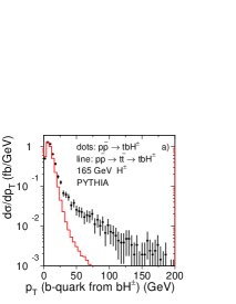
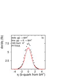
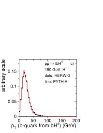
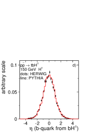
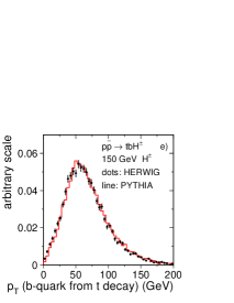
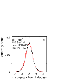
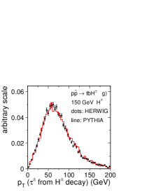
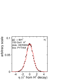
Figure 43: Distributions of charged Higgs boson selection variables at the parton level for $\sqrt{s}=1960$ GeV and $\tan\beta=20$ for HERWIG and PYTHIA. The variables are described in the text. In a) and b) the differences are mainly from top off-shellness effects. In c) to h) each pair of curves is normalised to an equal area. The error bars on the dots indicate the statistical uncertainty.

2.4 Conclusions

At Tevatron Run-II, about 1000 $\rm p\bar{p}\to tbH^{\pm}$ events per 1 fb^-1 at $\sqrt{s}=1960$ GeV could be produced for $m_{\rm H^{\pm}}=100$ GeV and $\tan\beta=20$, while about 100 events are expected for $m_{\rm H^{\pm}}=150$ GeV. These expected event rates will strongly be reduced when selection criteria are applied to separate signal and background events. For the default choices of mass and coupling parameters in HERWIG and PYTHIA we observe significant differences in the simulated total cross sections. We have also studied the shape of basic selection variable distributions and found good agreement between the HERWIG and PYTHIA parton level predictions in the $\rm p\bar{p}\to tbH^{\pm}$ process. In comparison with the $\rm p\bar{p}\rightarrow t\bar{t}\to tbH^{\pm}$ subprocess, which was used in previous HERWIG and PYTHIA versions, for $m_{\rm H^{\pm}}>160$ GeV the simulation of the full process results in significantly different distributions of $\rm tbH^{\pm}$ selection variables, mainly in the $p_{\rm T}$ distribution of the b-quark produced in association with the $\rm H^{\pm}$.

C. Extracting Higgs boson couplings from LHC data
M. Dührssen, S. Heinemeyer, H. Logan, D. Rainwater, G. Weiglein and D. Zeppenfeld

1 Introduction

LHC experiments have the capability to observe the Higgs boson in a variety of channels, in particular if its mass lies in the intermediate mass region, 114 GeV$<m_{H}\mathrel{\raise 1.29167pt\hbox{$<$\kern-7.5pt\lower 4.30554pt\hbox{$\sim$}}}200$ GeV, as suggested by direct searches [243] and electroweak precision data [244]. Once the Higgs boson is discovered, and its mass measured, one will want to gain as much information as possible on Higgs boson couplings to both gauge bosons and fermions. These measurements will provide crucial tests of the mass generation mechanism realized in nature.

The various Higgs couplings determine Higgs production cross sections and decay branching fractions. By measuring the rates of multiple channels, various combinations of couplings can be determined. A principal problem is that there is no technique analogous to the measurement of the missing mass spectrum at a linear collider [299] which would allow for a direct determination of the total Higgs production cross section. In addition, some Higgs decay modes cannot directly be observed at the LHC. For example, $H\to gg$ or decays into light quarks will remain hidden below overwhelming QCD dijet backgrounds. This implies that absolute measurements of (partial) decay widths are only possible with additional theoretical assumptions.

One possible strategy was outlined at Les Houches in 1999 [61, 77]. Assuming the absence of unexpected decay channels and a SM ratio of the $H\to b\bar{b}$ and $H\to\tau\tau$ partial widths, absolute measurements of $\Gamma(H\to WW/ZZ)$, $\Gamma(H\to\tau\tau)$, $\Gamma(H\to\gamma\gamma)$, $\Gamma(H\to gg)$ and of the top quark Yukawa coupling squared, $Y_{t}^{2}$, are possible, with errors in the 10–30% range.

Here we revisit the information which can be extracted at the LHC from rate measurements of an intermediate mass Higgs boson. We consider the expected accuracies at various stages of the LHC program: after 30 fb^-1 of low luminosity running (at $10^{33}\,{\rm cm}^{-2}{\rm sec}^{-1}$), 300 fb^-1 of high luminosity running (at $10^{34}\,{\rm cm}^{-2}{\rm sec}^{-1}$), and a mixed scenario where the vector boson fusion channels are assumed to suffer substantially from pile-up problems under high luminosity running conditions (making forward jet tagging and central jet veto fairly inefficient).

A rather model independent analysis, where only ratios of couplings (or partial widths) can be extracted, has been performed in Ref. [112]. Here we consider general multi-Higgs-doublet models (with or without additional Higgs singlets), in which the $HWW$ and $HZZ$ couplings are bounded from above by their SM values, i.e., we impose theoretically motivated constraints on these two couplings. These constraints are valid, in particular, for the Minimal Supersymmetric Standard Model (MSSM) and will sharpen the implications of LHC data for Higgs couplings very significantly.

An alternative approach is a fit of observed rates in the Higgs sector to specific models. Here we consider specific MSSM scenarios and use the $m_{h}^{\rm max}$ scenario of Ref. [169] as an example. The significance of deviations of the measured rates from SM predictions provide a measure of the sensitivity of LHC measurements in the Higgs sector. We discuss this approach in Section 4

2 Summary of Higgs boson channels

In order to determine the properties of a physical state such as a Higgs boson, one needs at least as many separate measurements as properties to be measured, although two or more measurements can be made from the same channel if different information is used, e.g., total rate and an angular distribution. Fortunately, the LHC will provide us with many different Higgs observation channels. In the SM there are four relevant production modes: gluon fusion (GF; loop-mediated, dominated by the top quark), also known as “inclusive” production; weak boson fusion (WBF), which has an additional pair of hard and far forward/backward jets in the final state; top-quark associated production ($t\bar{t}H$); and weak boson associated production ($WH,ZH$), where the weak boson is identified by its leptonic decay. 

Although a Higgs is expected to couple to all SM particles, not all its decays to these particles would be observable. Very rare decays (e.g., to electrons) would have no observable rate, and other modes are unidentifiable QCD final states (gluons or quarks lighter than bottom). In general, however, the LHC will be able to observe Higgs decays to photons, weak bosons, tau leptons and $b$ quarks, in the range of Higgs masses where the branching ratio (BR) in question is not too small.

For a Higgs in the intermediate mass range, the total width, $\Gamma$, is expected to be small enough to use the narrow-width approximation in extracting couplings. The rate of any channel (with the $H$ decaying to final state particles $dd$) is, to good approximation, given by

$$\sigma(H){\rm BR}(H\to dd)={\sigma(H)^{\rm SM}\over\Gamma_{p}^{\rm SM}}\cdot{\Gamma_{p}\Gamma_{d}\over\Gamma}\;,$$ (46)

where $\Gamma_{p}$ is the Higgs partial width involving the production couplings and where the Higgs branching ratio for the decay is written as ${\rm BR}(H\to dd)=\Gamma_{d}/\Gamma$. Even with cuts, the observed rate directly determines the product $\Gamma_{p}\Gamma_{d}/\Gamma$ (normalized to the calculable SM value of this product). The LHC will have access to (or provide upper limits on) combinations of $\Gamma_{g},\Gamma_{W},\Gamma_{Z},\Gamma_{\gamma},\Gamma_{\tau},\Gamma_{b}$ and the square of the top Yukawa coupling, $Y_{t}$. 

Since experimental analyses are driven by the final state observed, we classify Higgs channels by decay rather than production mode, and then discuss the different production characteristics as variants of the final state. However, some initial comments on production modes are in order. First, experimental studies mostly do not yet include the very large (N)NLO enhancements known for $gg\to H$ [25, 26, 27]. Even if background corrections are as large as for the signal, which they typically are not, the statistical significance of the GF channels will be greater than estimated by the current studies. Second, experimental studies do not consider WBF channels above 30 fb^-1 of integrated luminosity, because the efficiency to tag forward jets at high-luminosity LHC running is not yet fully understood. This is a very conservative assumption, which we comment on again later.

The literature on Higgs channels at LHC is extensive. We cite only those analyses which we use in our fits and accuracy estimates for coupling extractions. Mostly, these are recent experimental analyses which contain references to the earlier phenomenological proposals. In the discussion below, statements about Higgs rates typically refer to the SM-like case. Substantially suppressed branching ratios are possible beyond the SM and may change a measurement into an upper bound.

2.1 $H\to Z^{(*)}Z^{(*)}\to 4\ell$

Leptons are the objects most easily identified in the final state, so this decay is regarded as “golden” due to its extreme cleanliness and very low background. It is a rare decay due to the subdominance of $H\to ZZ$ relative to $H\to W^{+}W^{-}$, and because of the very small BR of $Z\to\ell^{+}\ell^{-}$. Fortunately, due to the possible decay to off-shell $Z$ bosons, a SM Higgs has non-negligible BR to $4\ell$ even for $M_{H}<2M_{Z}$, down to approximately 120 GeV.  Due to the low event rate, current studies concentrate on inclusive measurements which are dominated by GF. They provide information mainly on the product $\Gamma_{g}\Gamma_{Z}$.

The most advanced analysis for this channel [300] was made recently by ATLAS. (For an older CMS study, see [301]). Its principal improvement over previous studies is the full use of NLO results (the only study so far to do this) for both the dominant GF signal and its major backgrounds. Further improvements can be expected in the inclusion of off-shell contributions to the $gg\to ZZ^{(*)}$ background, for which ATLAS used an approximate K-factor.

By isolating the WBF contribution one obtains some independent information on the product $\Gamma_{W,Z}\Gamma_{Z}$, in particular if high-luminosity running can be exploited for this channel. We use the rates of Ref. [112] for our fits.

2.2 $H\to\gamma\gamma$

Photons are also readily identifiable, but are more difficult than leptons to measure because of a large, non-trivial background from jets faking photons. Higgs photonic decay is loop-induced and therefore rare, even more so because of destructive interference between the top-quark and $W$ loops. This is in some sense advantageous, because this decay mode is then sensitive to variations in the weak gauge and top Yukawa couplings and additional particles in the loop. This decay is visible in the SM only for the lower Higgs mass range, 110 GeV$<M_{H}<150$ GeV.

Despite the difficulties of identifying photons, which are not yet fully understood for the LHC, especially for high-luminosity running, Higgs decays to photons should be observable in both GF [59, 302, 224] and WBF [303, 304], unless ${\rm BR}(H\to\gamma\gamma)$ is substantially smaller than in the SM. These channels measure the products $\Gamma_{g}\Gamma_{\gamma}$ and $\Gamma_{W,Z}\Gamma_{\gamma}$. The $H\to\gamma\gamma$ signals in $t\bar{t}H,WH$ and $ZH$ production [59, 305] are very weak, due to lack of events even at high-luminosity running, but could be used as supplemental channels, and would be especially useful if LHC observes a non-SM Higgs.

2.3 $H\to W^{+(*)}W^{-(*)}\to\ell^{+}\ell^{-}+/\!\!\!p_{T}$

This decay can be observed in GF [59, 108, 306] and WBF [242, 220] using $W^{+}W^{-}\to\ell^{+}\ell^{-}+/\!\!\!p_{T}$ final states, as well as in $t\bar{t}H$ associated production using combinations of multilepton final states [307]. The first two modes extract the products $\Gamma_{g}\Gamma_{W}$ and $\Gamma^{2}_{W}$ and are extremely powerful statistically, while the $t\bar{t}H$ mode can extract the top Yukawa coupling with high luminosity and once $\Gamma_{W}$ is known. All these channels are accessible over a wide range of Higgs masses, approximately 120 GeV$<M_{H}<200$ GeV. An additional study [308] for the $WH,H\to WW$ channel for $M_{H}>150$ GeV found only a very weak signal, less than $5\sigma$ even for 300 fb^-1 of data.

The GF mode should improve after NLO effects are included, although the backgrounds considered did not include off-shell $gg\to WW^{*}$. Also, the single-top background was conservatively overestimated. A reanalysis of this channel with updated simulation tools would be useful.

2.4 $H\to\tau^{+}\tau^{-}$

Observing Higgs decays to taus is not possible in GF because of serious background problems and because the invariant mass of a tau pair can be reconstructed only when they do not decay back-to-back, which leaves only GF events with sizable Higgs transverse momentum. Observation of $H\to\tau^{+}\tau^{-}$ is possible in WBF, however [242, 219], for Higgs masses below about 150 GeV. As the average Higgs $p_{T}$ in this production mode is ${\cal O}(100)$ GeV, the taus are only rarely produced back-to-back. This is a relatively rare decay mode, since BR($H\to\tau\tau$) is typically $5-10\%$ in this mass region and the taus decay further. At least one tau must decay leptonically, giving another small BR. Fortunately, the QCD background to taus is small, due to excellent fake jet rejection. While not a discovery channel, this channel is statistically quite powerful with only moderate luminosity, and thus becomes one of the more important decay modes in a couplings analysis. This channel measures the product $\Gamma_{W,Z}\Gamma_{\tau}$.

2.5 $H\to b\bar{b}$

Associated Higgs-$b$ quark production has too small a cross section in a SM-like Higgs sector to be observable, so the decay $H\to b\bar{b}$ is the only access to the $b$ Yukawa coupling. Because this decay mode dominates Higgs decays at low mass ($M_{H}<135$ GeV within the SM), an accurate measurement of the bottom Yukawa coupling is extremely important. Unfortunately, due to the typically large QCD backgrounds for $b$ jets, it is very difficult to observe this decay. The production modes $t\bar{t}H$ [309, 310, 311] and $WH$ [59, 222] might allow very rough measurements for such a light Higgs, but the statistical significances are quite low and the background uncertainties quite large; they are definitely high-luminosity measurements.

The $t\bar{t}H$ channel measures the product $Y_{t}^{2}\Gamma_{b}$, and so would require a separate, precise measurement of $Y_{t}$ to isolate $\Gamma_{b}$. For $WH$ production, the rate is proportional to $\Gamma_{W}\Gamma_{b}$. But here the $Wb\bar{b}$ continuum background has hitherto been underestimated since the NLO QCD corrections are very large and positive [216]. A veto on additional jets may help but requires another detector-level simulation; unfortunately, it would also increase the background uncertainty because additional jet activity has been calculated at LO only.

2.6 Other channels

The production and decay channels discussed above refer to a single Higgs resonance, with decay signatures which also exist in the SM. The Higgs sector may be much richer, of course. The MSSM with its two Higgs doublets predicts the existence of three neutral and one charged Higgs boson, and the LHC may be able to directly observe several of these resonances. Within SUSY models, additional decays, e.g., into very light super-partners, may be kinematically allowed. The additional observation of super-partners or of heavier Higgs bosons will strongly focus the theoretical framework and restrict the parameter space of a Higgs couplings analysis [312].

At the present time, even enumerating the possibilities is an open-ended task. For our present analysis we therefore ignore the information which would be supplied by the observation of additional new particles. Instead we ask the better defined question of how well LHC measurements of the above decay modes of a single Higgs resonance can determine the various Higgs boson couplings or partial widths.

3 Model assumptions and fits

In spite of the many decay channels discussed above, the LHC is faced with the challenge that not all Higgs decay modes can be detected directly (e.g., $H\to gg$ is deemed unobservable) or that some important decay rates, in particular $H\to b\bar{b}$, will suffer from large experimental uncertainties. In a model-independent analysis, the limited information which will be available then leads to strong correlations in the measurement of different Higgs couplings. These correlations mask the true precision of LHC measurements when the expected errors of particular observables like individual partial widths or branching ratios are considered.

The parameter correlations can be overcome by imposing theoretical constraints. One possible approach was suggested in Les Houches 1999 [61, 77]. Fixing the ratio $\Gamma_{b}/\Gamma_{\tau}$ to its SM value, the $H\to\tau\tau$ measurements can be used to pin down the poorly measured Higgs coupling to bottom quarks. Here we follow a different approach. We perform general fits to the Higgs couplings with a series of theoretical assumptions of increasing restrictiveness, starting with the constraint $\Gamma_{V}\leq\Gamma_{V}^{\rm SM}$ ($V=W,Z$) which is justified in any model with an arbitrary number of Higgs doublets (with or without additional Higgs singlets), i.e., it is true for the MSSM in particular.

Even without this constraint, the mere observation of Higgs production puts a lower bound on the production couplings and, thereby, on the total Higgs width. The constraint $\Gamma_{V}\leq\Gamma_{V}^{\rm SM}$, combined with a measurement of $\Gamma_{V}^{2}/\Gamma$ from observation of $H\to VV$ in WBF, then puts an upper bound on the Higgs total width, $\Gamma$. It is this interplay which provides powerful constraints on the remaining Higgs couplings.

3.1 Fitting procedure

Our analysis of expected LHC accuracies closely follows the work of Dührssen [112]. First, a parameter space (${\bf x}$) is formed of Higgs couplings together with additional partial widths to allow for undetected Higgs decays and additional contributions to the loop-induced Higgs couplings to photon pairs or gluon pairs due to non-SM particles running in the loops. Assuming that the measured values correspond to the SM expectations, a log likelihood function, $L({\bf x})$, is formed which, for a given integrated luminosity, is based on the expected Poisson errors of the channels listed in Sec. 2 and on estimated systematic errors [112]. These errors include a 5% luminosity error, uncertainties on the reconstruction/identification of leptons (2%), photons (2%), b-quarks (3%) and forward tagging jets and veto jets (5%), error propagation for background determination from side-band analyses (from 0.1% for $H\to\gamma\gamma$ to 5% for $H\to WW$ and $H\to\tau\tau$) and theoretical and parametric uncertainties on Higgs boson production (20% ggH, 15% ttH, 7% WH/ZH, 4% WBF) and decays (1%, as a future expectation).

As an alternative, in particular for the specific MSSM scenarios discussed in Sec. 4, a Gaussian approximation to the log likelihood function is used, i.e., a $\chi^{2}$ function is constructed from the same error assumptions that enter the log likelihood function. We have checked that the resulting accuracy estimates for coupling measurements are consistent for the two approaches.

Relative to SM expectations, the variation of either $2L({\bf x})$ or $\chi^{2}({\bf x})$ is then computed on this parameter space, and the surface of variations by one unit is traced out. The $1\sigma$ uncertainties in each parameter are determined by finding the maximum deviation of that parameter from its SM value that lies on the $\Delta\chi^{2}=1$ ($\Delta L=1/2$) surface. The procedure is repeated for each Higgs mass value in the range 110 GeV$\leq m_{H}\leq 190$ GeV in steps of 10 GeV.

We perform the fits under three luminosity assumptions for the LHC:

1. 30 fb^-1 at each of two experiments, denoted 2*30 fb^-1;

2. 300 fb^-1 at each of two experiments, of which only 100 fb^-1 is usable for WBF channels at each experiment, denoted 2*300 + 2*100 fb^-1;

3. 300 fb^-1 at each of two experiments, with the full luminosity usable for WBF channels, denoted 2*300 fb^-1.

The second case allows for significant degradation of the WBF channels in a high luminosity environment while the third case serves to motivate additional improvements in WBF studies at high luminosity.

3.2 General multi-Higgs-doublet model fits

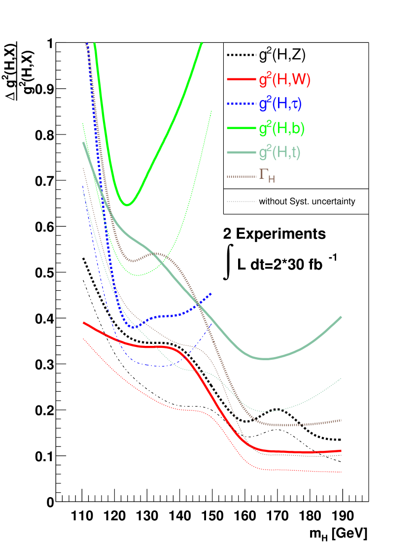
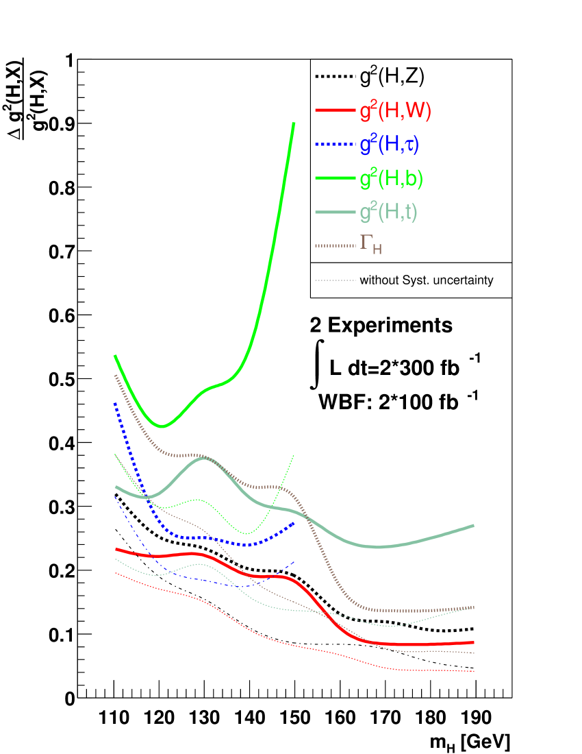
Figure 44: Relative precisions of fitted Higgs couplings-squared as a function of the Higgs mass assuming 30 fb^-1 at each of two experiments (left) and 300 fb^-1 at each of two experiments for all channels except WBF, for which 100 fb^-1 is assumed (right). Here we make the weak assumption that $g^{2}(H,V)<g^{2}(H,V,SM)+5\%$ ($V=W,Z$) but allow for new particles in the loops for $H\to\gamma\gamma$ and $gg\to H$ and for unobservable decay modes. See text for details.

We begin by fitting for the uncertainties in the Higgs couplings-squared in the most general scenario that we consider. We assume only that $g^{2}(H,W)<1.05*g^{2}(H,W,SM)$ and $g^{2}(H,Z)<1.05*g^{2}(H,Z,SM)$. Any model that contains only Higgs doublets and/or singlets will satisfy the relations $g^{2}(H,W)\leq g^{2}(H,W,SM)$ and $g^{2}(H,Z)\leq g^{2}(H,Z,SM)$. The extra 5% margin allows for theoretical uncertainties in the translation between couplings-squared and partial widths and also for small admixtures of exotic Higgs states, like SU(2) triplets. We allow for the possibility of additional particles running in the loops for $H\to\gamma\gamma$ and $gg\to H$, fitted by a positive or negative new partial width to these contributions. This new partial width for $H\to\gamma\gamma$ is most tightly constrained for 120 GeV$\mathrel{\raise 1.29167pt\hbox{$<$\kern-7.5pt\lower 4.30554pt\hbox{$\sim$}}}m_{H}\mathrel{\raise 1.29167pt\hbox{$<$\kern-7.5pt\lower 4.30554pt\hbox{$\sim$}}}140$ GeV, being less than $\pm(25-35)\%$ of $\Gamma_{\gamma}^{\rm SM}$ for 2*30 fb^-1 and $\pm(10-15)\%$ for 2*300 + 2*100 fb^-1. The new partial width for $gg\to H$ is less well constrained, being less than $\pm(30-90)\%$ of $\Gamma_{g}^{\rm SM}$ for 2*30 fb^-1 and $\pm(30-45)\%$ for 2*300 + 2*100 fb^-1 over the whole range of Higgs masses. Additional decays of the Higgs boson are fitted with a partial width for undetected decays. This undetected partial width can be constrained to be less than $15-55\%$ of the total fitted Higgs width for 2*30 fb^-1 and $15-30\%$ for 2*300 + 2*100 fb^-1, at the $1\sigma$ level. This undetected partial width is most tightly constrained for Higgs masses above 160 GeV.

The resulting parameter precisions are shown in Fig. 44 as a function of Higgs mass for the 2*30 fb^-1 and 2*300 + 2*100 fb^-1 luminosity scenarios. For the latter case, typical accuracies range between 20 and 30% for Higgs masses below 150 GeV. Above $W$-pair threshold the measurement of the then dominant $H\to WW,ZZ$ partial widths improves to the 10% level. The case of 2*300 fb^-1 yields only small improvements over the right-hand panel in Fig. 44, except in the case of $g^{2}(H,\tau)$ which shows a moderate improvement. This can be understood because the $H\to\tau\tau$ decay is measured only in WBF, and $g(H,\tau)$ does not have a large effect on the Higgs total width or loop-induced couplings.

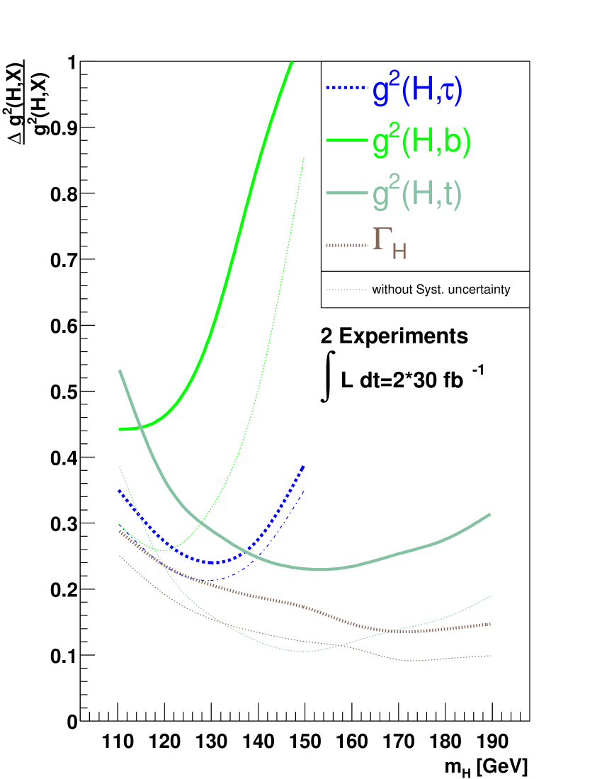
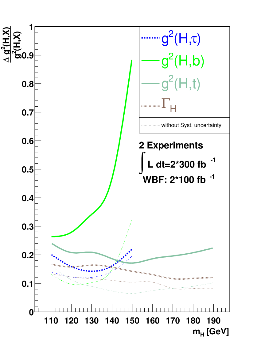
Figure 45: As in Fig. 44, but with more restrictive assumptions. Here we assume that $g^{2}(H,W)=g^{2}(H,W,SM)\pm 5\%$ and $g^{2}(H,W)/g^{2}(H,Z)=g^{2}(H,W,SM)/g^{2}(H,Z,SM)\pm 1\%$. We also assume that no new particles run in the loops for $H\to\gamma\gamma$ and $gg\to H$, so that these couplings are fixed in terms of the couplings of the SM particles in the loops. As in Fig. 44, additional decays of the Higgs boson are fitted with a partial width for undetected decays (not shown).

The results shown in Fig. 44 reflect present understanding of detector effects and systematic errors. One should note that improved selection and higher acceptance will decrease the statistical errors. At least as important is work on the reduction of systematic errors. In Fig. 44, the thin lines show expectations with vanishingly small systematics: systematic errors contribute up to half the total error, especially at high luminosity.

3.3 SU(2) constraints and SM loops

The theoretical constraints used so far have been very moderate. If, in addition to the requirement that $g^{2}(H,W)<g^{2}(H,W,SM)+5\%$ and $g^{2}(H,Z)<g^{2}(H,Z,SM)+5\%$, we assume that no new non-SM particles run in the loops for $H\to\gamma\gamma$ and $gg\to H$ (which is approximately fulfilled for the MSSM with a not too light spectrum), the precision of the coupling measurements improves only slightly, with the only noticeable improvement for Higgs masses below 120 GeV.

Another small improvement is achieved by restricting the $W$ and $Z$ couplings to their SM ratio. Within the multi-Higgs-doublet models considered throughout, SU(2) symmetry relates these two couplings. It thus is natural to forgo an independent measurement of their ratio and to rather assume that

$$g^{2}(H,W)/g^{2}(H,Z)=g^{2}(H,W,SM)/g^{2}(H,Z,SM)\pm 1\%\;.$$ (47)

Within the MSSM, this coupling ratio is indeed very close to its SM value. Over most of the MSSM parameter space even the individual $hVV$ couplings will be close to their SM values since decoupling sets in rapidly once the mass of the $CP$-odd Higgs boson becomes large, $m_{A}\mathrel{\raise 1.29167pt\hbox{$>$\kern-7.5pt\lower 4.30554pt\hbox{$\sim$}}}200$ GeV. This motivates a fit where in addition to Eq. 47 we assume

$$g^{2}(H,W)=g^{2}(H,W,SM)\pm 5\%\;.$$ (48)

We again assume that no new non-SM particles run in the loops for $H\to\gamma\gamma$ and $gg\to H$. However, additional decays of the Higgs boson are fitted with a partial width for undetected decays. The constraints on this undetected partial width are essentially the same as in our least constrained fit. The resulting parameter precisions are shown in Fig. 45 and reach 10–20% over the entire intermediate Higgs mass range for the 2*300 + 2*100 fb^-1 luminosity scenario.

Loosening assumptions slightly, by allowing non-SM particles to contribute to the $H\to\gamma\gamma$ partial width, has a noticeable effect on the coupling determination only for $m_{H}\mathrel{\raise 1.29167pt\hbox{$<$\kern-7.5pt\lower 4.30554pt\hbox{$\sim$}}}120$ GeV. For example, for the 2*300 + 2*100 fb^-1 luminosity scenario, the precision on $g^{2}(H,\tau)$, $g^{2}(H,b)$ and the Higgs total width at $m_{H}=110$ GeV jump to about 40%.

4 Higgs couplings within the MSSM

A plausible scenario is that one or several Higgs bosons will be discovered at the LHC together with evidence for supersymmetry (SUSY) at the TeV scale. Once SUSY has been confirmed, we are led to analyzing the Higgs sector in terms of a two Higgs doublet model with MSSM constraints.

For the sake of brevity let us assume that the pseudoscalar Higgs and the charged Higgs are fairly heavy ($m_{A}\mathrel{\raise 1.29167pt\hbox{$>$\kern-7.5pt\lower 4.30554pt\hbox{$\sim$}}}150$ GeV, and they may, but need not, have been observed directly) and that the observed sparticles’ masses ensure that the light Higgs boson can decay into only SM particles. Then the light Higgs that we consider here will have couplings to the $W$ and $Z$ which are suppressed by the same factor $\sin(\alpha-\beta)$ compared to SM strength, and Higgs couplings to fermions in addition depend on $\tan\beta=v_{2}/v_{1}$ and $\Delta_{b}$ [313], which incorporates non-universal loop corrections to the $h\bar{b}b$ coupling. A fit of the Higgs couplings can then be performed in terms of this reduced parameter set. Obviously this analysis falls within the $g_{V}\leq g_{V}^{\rm SM}$ analysis described in the previous section. Upper bounds on the expected measurement errors for MSSM partial widths can hence be derived from Fig. 44, while Fig. 45 gives an estimate of errors which can be expected for $m_{A}\mathrel{\raise 1.29167pt\hbox{$>$\kern-7.5pt\lower 4.30554pt\hbox{$\sim$}}}200$ GeV.

Figure 46: Fit within the MSSM $m_{h}^{\rm max}$ scenario in the $M_{A}$–$\tan\beta$ plane for three luminosity scenarios. The two panels show the region (to the left of the curves) in which a $\geq 5\sigma$ ($\Delta\chi^{2}\geq 25$) or $\geq 3\sigma$ ($\Delta\chi^{2}\geq 9$) discrepancy from the SM can be observed. The mostly-horizontal dotted lines are contours of $m_{h}$ in steps of 5 GeV.

A quantitative, global measure of how well the LHC can distinguish the SM from a specific MSSM scenario is provided by a $\chi^{2}$-analysis of the deviations expected for a specific SUSY model. As a specific example we consider the $m_{h}^{\rm max}$ scenario of Ref. [169]. We calculate the mass and branching fractions of the MSSM Higgs boson using HDECAY3.0 [165], using the FeynHiggsFast1.2.2 [314, 315] option to compute the MSSM Higgs masses and couplings. Assuming that, for a given $m_{A}$ and $\tan\beta$, the corresponding SUSY model is realized in nature, we may ask at what significance the SM can be ruled out from $h$ measurements alone. The resulting contours are shown in Fig. 46 for the three luminosity assumptions defined in Sect. 3.1. In the areas to the left of the contours the SM can be rejected with more than 5$\sigma$ or 3$\sigma$ significance, respectively.

The $\chi^{2}$ definition in Fig. 46 assumes the same systematic errors as our analysis in Sec. 3 Event rates and resulting statistical errors, however, are those expected for the MSSM. It should be noted that the position of the contours shifts only very little if one assumes SM rates to be observed. The contours do shift significantly, however, when using different SUSY scenarios: other SUSY parameters can have a large effect on the relation of $m_{h}$, $m_{A}$, $\tan\beta$ and Higgs couplings and, hence, an indirect determination of $m_{A}$ from observed deviations in light Higgs couplings is problematic without significant input from other direct SUSY observations at the LHC.

5 Summary

Measurements in the Higgs sector are expected to provide many complementary signatures after several years of LHC running. Combining these measurements allows one to extract information on Higgs partial widths and Higgs couplings to fermions and gauge bosons. Because significant contributions from unobservable channels cannot easily be ruled out at the LHC, model-independent analyses produce large correlations between extracted partial widths. A reduction of correlations and hence smaller errors on particular couplings can be achieved with a variety of theory assumptions. In this contribution we have analyzed the constraints expected in generic multi Higgs doublet models, namely that $HVV$ couplings cannot be larger than within the SM. Within such models, the LHC can measure Higgs couplings to top, tau, $W$ and $Z$ with accuracies in the 10–30% range, once 300 fb^-1 of data have been collected.

Within the MSSM, significant deviations in the Higgs sector should be observable at the LHC, provided that the charged and the pseudoscalar Higgs masses are not too heavy, i.e., that decoupling is not yet completely reached. Within the $m_{h}^{\rm max}$ scenario and with 300 fb^-1 of data, the LHC can distinguish the MSSM and the SM at the 3$\sigma$ level up to $m_{A}\simeq 450$ GeV and with 5$\sigma$ significance up to $m_{A}\simeq 350$ GeV. The LHC will thus provide a surprisingly sensitive first look at the Higgs sector, even though it cannot match precision and the model-independence of analyses which are expected for a linear $e^{+}e^{-}$ collider [316].

D. Estimating the Precision of a tan$\beta$ Determination with H/A $\rightarrow\tau\tau$ and H${}^{\pm}\rightarrow\tau\nu$ in CMS
R. Kinnunen, S. Lehti, F. Moortgat, A. Nikitenko and M. Spira

1 Introduction

The Higgs mechanism is a cornerstone of the Standard Model (SM) and its supersymmetric extensions. Therefore, the search for Higgs bosons is one of the top priorities at future high-energy experiments. Since the minimal supersymmetric extension of the Standard Model (MSSM) requires the introduction of two Higgs doublets in order to preserve supersymmetry, there are five elementary Higgs particles, two CP-even (h,H), one CP-odd (A) and two charged ones (H^±). At lowest order all couplings and masses of the MSSM Higgs sector are determined by two independent input parameters, which are generally chosen as tan$\beta=v_{2}/v_{1}$, the ratio of the two vacuum expectation values $v_{1,2}$, and the pseudoscalar Higgs-boson mass m_A. At LO the light scalar Higgs mass m_h has to be smaller than the Z-boson mass m_Z. However, this upper bound is significantly enhanced by radiative corrections, the leading part of which grows with the fourth power of the top mass and logarithmically with the stop masses. Including the one-loop and dominant two-loop corrections the upper bound is increased to m${}_{\rm h}\mbox{\raisebox{-2.58334pt}{~{}$\stackrel{{\scriptstyle<}}{{\sim}}$~{}}}135$ GeV$/c^{2}$ [252]. The negative direct searches for the Higgsstrahlung processes $e^{+}e^{-}\to\rm Zh/ZH$ and the associated production $e^{+}e^{-}\to\rm Ah/AH$ yield lower bounds of m${}_{\rm h,H}>91.0$ GeV$/c^{2}$ and m${}_{\rm A}>91.9$ GeV$/c^{2}$. The range $0.5<$tan$\beta<2.4$ in the MSSM is excluded for m${}_{\rm t}=174.3$ GeV$/c^{2}$ by the Higgs searches at the LEP2 experiments [317].

Thus, one of the most important parameters to be determined in the Minimal Supersymmetric Standard Model (MSSM) as well in a general type-II Two-Higgs Doublet Model (2HDM) is tan$\beta$. In the MSSM tan$\beta$ plays a crucial role, since it characterizes the relative fraction of the two Higgs boson doublets contributing to the electroweak symmetry breaking. Consequently, it enters in all sectors of the theory. For small tan$\beta$, it may be possible to determine the value of tan$\beta$ within the sfermion or neutralino sector [318, 319]. For large tan$\beta$ this method has not been found to be effective. However, in this regime, there are good prospects to measure the value of tan$\beta$ by exploiting the Higgs sector [320].

At large tan$\beta$ neutral and charged Higgs boson production is dominated by the bremsstrahlung processes $\rm gg\rightarrow b\bar{\rm b}H/A$, gb $\rightarrow$ tH^± and gg $\rightarrow$ tbH^±. The dominant parts of the production cross sections are proportional to tan${}^{2}\beta$. Due to this feature the uncertainty of the tan$\beta$ measurement is only half of the uncertainty of the rate measurement. In the MSSM the supersymmetric loop corrections introduce an additional tan$\beta$ dependence to the cross section [321], but they can be absorbed in an effective parameter tan$\beta_{\rm eff}$, since the dominant terms which are enhanced by tan$\beta$ correspond to emission and reabsorption of virtual heavy supersymmetric particles at the bottom Yukawa vertex, which are confined to small space-time regions compared with QCD subprocesses involving massless gluons. The subleading terms are small. The dominant terms are universal contributions to the bottom Yukawa coupling [321]. This implies that the method described below determines this effective parameter tan$\beta_{\rm eff}$ in the MSSM. The extraction of the fundamental tan$\beta$ parameter requires additional knowledge of the sbottom and gluino masses as well as the $\mu$ parameter. These corrections are in general absent in a 2HDM so that in these models the extracted value belongs to the fundamental tan$\beta$ parameter. The H/A $\rightarrow\mu\mu$ [322] and H/A $\rightarrow\tau\tau$ decay channels have been identified as the most promising for the searches of the heavy neutral MSSM Higgs boson H and A at large tan$\beta$. The final states $\rm e\mu$, $\ell\ell$ ($\rm\ell\ell=e\mu,ee,\mu\mu$) [323], lepton+jet [324] and two-jets [325] have been investigated for the H/A $\rightarrow\tau\tau$ decay mode. For heavy charged Higgs bosons the H${}^{\pm}\rightarrow\tau\nu$ decay channel in fully hadronic events (both $\tau$ and top decaying into hadrons) has been found to yield the largest parameter reach and a clean signature [326]. For the MSSM SUSY parameters, the following values are taken: M₂ = 200 GeV/$c^{2}$, $\mu$ = 300 GeV/$c^{2}$, M${}_{\tilde{\rm g}}$ = 800 GeV/$c^{2}$, M${}_{\tilde{\rm q},{\tilde{\ell}}}$ = 1 TeV/$c^{2}$ and A_t is set to 2450 GeV/$c^{2}$. The top mass is set to 175 GeV/$c^{2}$. The Higgs boson decays to SUSY particles are allowed.

In this work the theoretical uncertainty of the cross section and the branching ratio, the uncertainty of the luminosity measurement and statistical errors are taken into account. The uncertainty of the next-to-leading order (NLO) cross sections for the gg $\rightarrow$ b$\overline{\rm b}$H/A/h and gb $\rightarrow$ tH^± processes has been shown to be 20–30% for the total rate [327, 328]. However, it depends on the transverse momentum range of the spectator b quarks and reduces to 10–15% with the requirement of p${}_{\rm T}^{\rm b,\bar{\rm b}}\mbox{\raisebox{-2.58334pt}{~{}$\stackrel{{\scriptstyle>}}{{\sim}}$~{}}}$ 20 GeV/$c$ [327, 329, 330]. The uncertainty of the branching ratio BR(H/A$\rightarrow\tau\tau$) related to the uncertainties of the SM input parameters is about 3%. We have not taken into account the uncertainties related to the MSSM parameters, but kept them fixed at our chosen values. We only vary the pseudoscalar mass m_A and tan$\beta$. A 5% uncertainty of the luminosity measurement was taken. The precision of the mass measurement in H/A$\rightarrow\tau\tau$ is estimated and taken into account in the precision of the tan$\beta$ determination. The uncertainty of the background estimation as well as the uncertainty of the signal selection efficiency have not yet been taken into account in this study. We expect, however, that the background uncertainty and uncertainty of the signal selection will be of the order of 5 %.

In this work the accuracy of the tan$\beta$ measurement is estimated in the H/A $\rightarrow\tau\tau$ and H${}^{\pm}\rightarrow\tau\nu$ decay channels by exploiting the studies of Refs. [323, 325, 326]. The discovery reach for the lepton+jet final state from H/A $\rightarrow\tau\tau$, described in Ref. [324], is re-evaluated and used in the tan$\beta$ measurement. The event rates for the gb $\rightarrow$ tH^±, H${}^{\pm}\rightarrow\tau\nu$ channel are also updated according to the recent theoretical calculations of the cross section [328].

2 Transverse momentum of b quarks in $\rm g\rm g\rightarrow\rm b\bar{\rm b}H/A$

Higgs boson production in the $\rm gg\rightarrow\rm b\bar{\rm b}H/A$ process was obtained with the PYTHIA [203, 277] two-to-three processes 181 and 186 and with the PYTHIA6.158 default values for the parton distribution functions and the renormalization and factorization scales. No cut on the transverse momentum of the b quarks has been applied at the generation level but $\rm E_{\rm T}^{\rm jet}>$ 20 GeV is used for the b-jet identification in the event analysis. Therefore it is important to know how well PYTHIA describes the $\rm p_{\rm T}$ spectrum of the b quarks compared to the NLO calculations [331] in order to estimate how well the efficiency of the event selections can be trusted. Comparizon was made for the SM process $\rm gg\rightarrow b\bar{b}h$ (PYTHIA process 121) with Higgs mass of 120 GeV/$c^{2}$. The PYTHIA and the NLO cross sections are compared in Table 7 as a function of a cut on the transverse momentum of the b quark with highest $\rm p_{\rm T}$. In PYTHIA as well as in the NLO calculations the b quark momentum was taken after gluon radiation. The total PYTHIA cross sections (p${}_{\rm T}>0$) were normalized to the total NLO cross sections. The agreement between the PYTHIA and the NLO values turns out to be at the level of 5–10%. The statistical uncertainties of the PYTHIA cross sections are shown, too. For completeness the PYTHIA LO cross sections are also compared to the corresponding theoretical LO calculation (the lower two rows in Table. 7). In this case the PYTHIA b quark was taken before gluon radiation. Good agreement within 1–2 % has been obtained.

pT cut	0 GeV/c	10 GeV/c	20 GeV/c	30 GeV/c	40 GeV/c	50 GeV/c
$\sigma_{\rm NLO}$ (pb)	734	507	294	173	106	68
$\sigma_{\rm PYTHIA}$ (pb)	734	523 $\pm$ 3	275 $\pm$ 3	156 $\pm$ 3	92 $\pm$ 2	60 $\pm$ 2
$\sigma_{\rm LO}$ (pb)	528	393	241	152	102	71
$\sigma_{\rm PYTHIA}$ (pb)	528	407 $\pm$ 2	245 $\pm$ 3	154 $\pm$ 2	101 $\pm$ 2	70 $\pm$ 2

Table 7: Comparison of the NLO and LO cross sections to the PYTHIA cross sections as a function of the cut on the transverse momentum of the b quark with highest $\rm p_{\rm T}$. The total PYTHIA cross sections ($\rm p_{\rm T}>$ 0) are normalized to the corresponding NLO(LO) cross sections.

Figure 47: The 5$\sigma$-discovery potential for the heavy neutral MSSM Higgs bosons as a function of $\rm m_{\rm A}$ and tan$\beta$ with maximal stop mixing for 30 fb^-1. The H/A $\rightarrow\mu\mu$ and H/A $\rightarrow\tau\tau\rightarrow$ two-jet channels are shown for 60 fb^-1.

Figure 48: The 5$\sigma$-discovery potential for the charged Higgs bosons in the H${}^{\pm}\rightarrow\tau\nu$ decay channel as a function of $\rm m_{\rm A}$ and tan$\beta$ with maximal stop mixing for 30 fb^-1.

3 Event selections and expected discovery reaches

If the Higgs boson is detected with high enough signal significance, it is possible to count events in order to measure the value of tan$\beta$. The 5$\sigma$-discovery potential for the H/A/h $\rightarrow\tau\tau$ decay channels with the e$\mu$, $\ell\ell$ and lepton+jet final states for 30 fb^-1 and with the two-jet final state for 60 fb^-1 is shown in Figure 48. The 5$\sigma$-discovery reaches of the H/A $\rightarrow\mu\mu$ decay channel with 60 fb^-1 and of the H $\rightarrow\tau\tau\rightarrow$ lepton+jet channel in the weak gauge boson fusion with 30 fb^-1 are also depicted in the figure. Figure 48 presents the 5$\sigma$-discovery potential for the charged Higgs bosons in the H${}^{\pm}\rightarrow\tau\nu$ decay channel for 30 fb^-1. In these regions of the parameter space the value of tan$\beta$ can be determined by counting the neutral and charged Higgs bosons.

3.1 Neutral Higgs bosons

The event selections for the two-lepton (e$\mu$ and $\ell\ell$), lepton+jet ($\ell$j) and two-jet (jj) final states from H/A/h$\rightarrow\tau\tau$ are described in detail in Refs. [323, 324, 325]. The branching ratios into these final states are shown in Table 8. The discovery potential in the H/A/h$\rightarrow\tau\tau\rightarrow$ lepton+jet channel is re-evaluated using the cross sections of Ref. [332] and with updated $\tau$ selection and b-tagging efficiencies. Unlike Ref. [324], the recent analysis is extended to large Higgs boson masses, and a 5$\sigma$ reach up to m${}_{\rm A}\sim$ 650 GeV/$c^{2}$ at tan$\beta\sim$ 50 is obtained. The details will be described in an upcoming note.

Final state	branching ratio
H/A/h$\rightarrow\tau\tau\rightarrow$ e$\mu$+X	$\sim$6.3%
H/A/h$\rightarrow\tau\tau\rightarrow\ell\ell$+X	$\sim$12.5%
H/A/h$\rightarrow\tau\tau\rightarrow\ell$j+X	$\sim$45.6%
H/A/h$\rightarrow\tau\tau\rightarrow$ jj+X	$\sim$41.5%

Table 8: The branching ratios into final states $\tau\tau\rightarrow$X.

Figure 49: Reconstructed $\tau\tau$ invariant mass in the e$\mu$ final state in the H/A/h $\rightarrow\tau\tau$ signal (dark) and in the total background (light) with mA = 200 GeV/$c^{2}$ and tan$\beta$ = 20 for 30 fb-1.	Figure 50: Reconstructed $\tau\tau$ invariant mass in the $\ell\ell$ final state in the H/A/h $\rightarrow\tau\tau$ signal (dark) and in the total background (light) with mA = 200 GeV/$c^{2}$ and tan$\beta$ = 20 for 30 fb-1.
Figure 51: Reconstructed $\tau\tau$ invariant mass in the lepton+jet final state in the H/A/h $\rightarrow\tau\tau$ signal (dark) and in the total background (light) with mA = 200 GeV/$c^{2}$ and tan$\beta$ = 20 for 30 fb-1.	Figure 52: Reconstructed $\tau\tau$ invariant mass in H/A $\rightarrow\tau\tau\rightarrow$ 2 jets (dark), in the total background (light) and in the multi-jet background (dashed) with mA = 500 GeV/$c^{2}$ and tan$\beta$ = 30 for 60 fb-1.

The common backgrounds for all the H/A$\rightarrow\tau\tau$ channels are the Z,$\gamma^{*}\rightarrow\tau\tau$ Drell-Yan process, $\rm t\bar{\rm t}$ production with real and fake $\tau$’s and single top production (Wt). The channels with leptons in the final state suffer from the $\rm b\bar{\rm b}$ background, and the final states with hadronic $\tau$ decays are plagued by the W+jet background. For fully hadronic final states with both $\tau$’s decaying hadronically there is in addition the QCD multi-jet background with jets faking $\tau$’s, and for the H/A$\rightarrow\tau\tau\rightarrow\ell\ell$+X channel there is the additional background from Z,$\gamma^{*}$ decaying to electron and muon pairs.

The hadronic Tau Trigger for the two-jet final state was studied with full simulation in Ref. [325, 333]. For the e$\mu$, $\ell\ell$ and the $\ell$j final states the trigger was simulated by selecting the kinematic cuts above the trigger thresholds, and taking the trigger efficiencies from Ref. [333]. The used triggers were the Inclusive muon trigger with efficiency 0.9*0.97*0.97 (trigger threshold effect*$\mu$ reconstruction efficiency* calorimetric isolation), the Di-electron trigger with efficiency 0.95*0.872*0.946 per electron (trigger threshold effect*Level-1 e efficiency*Level-2.5 e efficiency) and e-$\tau$jet trigger with efficiency 0.95*0.872*0.77*0.95 (e trigger threshold effect*Level-1 e efficiency*HLT e efficiency*$\tau$ trigger threshold effect). The backgrounds were suppressed with lepton tracker isolation, $\tau$ jet identification, $\tau$ tagging with impact parameter, b tagging and jet veto. The $\tau$ jet identification [325] selects collimated low multiplicity jets with high p_T charged particles. The hadronic jets are suppressed by a factor of $\sim$ 1000. Tau tagging [323] exploits the short but measurable lifetime of the $\tau$: the decay vertex is displaced from the primary vertex. For b tagging the B hadron lifetime is used to distinguish the associated b jets from c jets and light quark/gluon jets. B tagging suppresses efficiently the Drell-Yan and QCD multi-jet backgrounds by a factor of $\sim$ 100, but it also suppresses the Higgs boson production with no associated b jets. The jet veto is directed against the $\rm t\bar{\rm t}$ and Wt backgrounds, in which the jets are more energetic and easier to reconstruct and to b-tag compared to jets associated with the signal. Rejecting events with more than one jet (including the b jet and not counting $\tau$’s) suppresses the $\rm t\bar{\rm t}$ background by a factor of $\sim$ 5 [325].

Despite several neutrinos in all the H/A$\rightarrow\tau\tau$ final states the Higgs boson mass can be reconstructed. The effective $\tau\tau$ mass is evaluated assuming that the neutrinos are emitted along the measured $\tau$ decay products. The neutrino energies are estimated by projecting the missing energy vector onto the neutrinos. Uncertainties in the missing energy measurement can lead to negative neutrino energies. A significant fraction of the signal events is lost, when positive neutrino energies are required, but the backgrounds from $\rm t\bar{\rm t}$, Wt and QCD multi-jet events are suppressed, since for these backgrounds the neutrinos are generally not emitted along the true or fake $\tau$’s. The mass resolution can be improved efficiently with a cut in the $\Delta\phi$ or space angle between the two $\tau$’s. For the two-jet final state in Ref. [325] a mass reconstruction efficiency of 53% has been obtained with the cut $\Delta\phi<$ 175^o and requiring one b jet with $\rm E_{\rm T}>$ 30 GeV. The reconstructed Higgs boson mass is shown in Figs. 52 to 52 for the four $\tau\tau$ final states. The reconstructed mass peak is a superposition of the H and A signals. In the region m${}_{\rm A}\mbox{\raisebox{-2.58334pt}{~{}$\stackrel{{\scriptstyle<}}{{\sim}}$~{}}}$ 130 GeV/$c^{2}$ the contribution from the lightest Higgs boson h cannot be separated in these channels and is also included in the signal event rates.

A 5$\sigma$-discovery reach combining the $\rm e\mu$, lepton+jet and two-jet final states from the H/A$\rightarrow\tau\tau$ decay channel is also shown in Fig. 48. The combined reach is evaluated by adding the number of signal and background events from the three final states in a given (m_A, tan$\beta$) point. However, this method can lead to an unsatisfactory result as the analysis of these final states has been optimized to reach the best possible signal significance which has led to different background levels. For example at low values of m_A and tan$\beta$ the signal for the H/A$\rightarrow\tau\tau\rightarrow\ell\ell$+X channel [323] suffers from a significantly larger Drell-Yan backgound than that for the H/A$\rightarrow\tau\tau\rightarrow$ lepton+jet channel. If the $\ell\ell$ final state is included, the combined reach is smaller than that from the lepton+jet final state alone.

3.2 Charged Higgs bosons

The production of heavy charged Higgs bosons has been studied in the gb $\rightarrow$ tH^±, H${}^{\pm}\rightarrow\tau\nu$ channel with hadronic $\tau$ decays in Ref. [326]. The W+jet and QCD multi-jet backgrounds have been suppressed by b tagging and reconstruction of the associated top quark. To suppress the t$\overline{\rm t}$ and Wt backgrounds with genuine $\tau$’s, the helicity correlations have been exploited by requiring at least 80% of the $\tau$-jet energy to be carried by a single charged pion. In purely hadronic final states the transverse Higgs boson mass can be reconstructed from the $\tau$ jet and the missing transverse energy, with an endpoint at m${}_{\rm H^{\pm}}$ for the signal and at m_W for the t$\overline{\rm t}$, Wt and W+jet backgrounds.

Figure 53: The inclusive production cross section $gb\to\rm tH^{\pm}$ at the LHC for m${}_{\rm H^{\pm}}=300$ GeV/$c^{2}$ as a function of tan$\beta$ from Ref. [328]. The dashed and solid curves present the consistent leading order and next-to-leading order results. The dotted line depicts the cross section with the bottom Yukawa coupling defined (inappropriately) in terms of the bottom pole mass and thus illustrate the enhancement through large logarithms. The range for the next-to-leading order result is given for $\mu_{F}=\mu_{R}=m_{\rm av}/4\cdots 4m_{\rm av}$ with m${}_{\rm av}=(\rm m_{\rm H^{\pm}}+m_{\rm t})/2$ denoting the average mass of the produced particles.

In Ref. [326] the PYTHIA estimates were used for the cross sections and branching ratios. Recently, detailed theoretical LO and NLO calculations have been published on the charged Higgs boson production at the LHC [328]. These calculations show significantly lower LO production cross sections especially for light charged Higgs bosons than those used in Refs. [326, 334]. Figure 53 shows the cross section for gb $\rightarrow$ tH^± at m${}_{\rm H^{\pm}}$ = 300 GeV/$c^{2}$ as a function of tan$\beta$ from Ref. [328]. The scale dependence of the LO cross section originating from the Yukawa coupling in the production mechanism is large at large tan$\beta$. The LO cross section of Ref. [328] at m${}_{\rm H^{\pm}}\sim$ 200 GeV/$c^{2}$ calculated with running b quark mass is a factor of $\sim$ 1.7 lower than that used in Ref. [326]. At m${}_{\rm H^{\pm}}\sim$ 600 GeV/$c^{2}$ the difference reduces to 10%. The H${}^{\pm}\rightarrow\tau\nu$ branching ratio was also overestimated in Ref. [326] by about 20% at m${}_{\rm H^{\pm}}$ = 200 GeV/$c^{2}$. The 5$\sigma$-discovery reach in Fig. 48 is shown with updated cross sections [328] and branching ratios [165]. The statistical significance is calculated with Poisson statistics. The reconstructed transverse mass is shown in Fig. 55.

Figure 54: Transverse mass reconstructed from the $\tau$ jet and $\rm E_{\rm T}^{\rm miss}$ in the $\rm gg\rightarrow\rm tH^{\pm}$, $\rm H^{\pm}\rightarrow\tau\nu_{\tau}$ with $\rm m_{\rm H^{\pm}}$ = 200 GeV/$c^{2}$ and tan$\beta$ = 30 for 30 fb-1.

Figure 55: Cross section times branching ratio for $\rm gg\rightarrow b\bar{b}H/A,H/A\rightarrow\tau\tau$ calculated with the programs of Ref. [332].

4 Calculation of the tan$\beta$ measurement uncertainty

The accuracy of the tan$\beta$ measurement is due to the statistical uncertainty of event rates, the systematic uncertainty from the luminosity measurement and the theoretical uncertainty of the cross section calculation. The associated Higgs boson production cross sections for $\rm gg\rightarrow b\bar{\rm b}H/A$ and gb $\rightarrow$ tH^± are approximately proportional to tan${}^{2}\beta$ at large tan$\beta$ due to the dominance of the bottom Yukawa coupling. The loop corrections introduce some additional tan$\beta$ dependence to the cross section, but they can be absorbed in an effective parameter tan$\beta_{eff}$ [321]. The results obtained in this analysis correspond to this effective parameter. The extraction of the fundamental MSSM tan$\beta$ value is beyond the scope of this work.

The branching ratio BR(H/A $\rightarrow\tau\tau$) is approximately constant at large tan$\beta$. At large tan$\beta$ the total decay width is dominated by Higgs boson decays to heavy down type fermions, $\tau^{+}\tau^{-}$ and $b\bar{b}$ pairs, for which the decay widths have similar tan$\beta$ dependence. If the SUSY corrections, which are different for the bottom and $\tau$ Yukawa couplings, are not large, the tan$\beta$ dependence cancels out in the ratio $\Gamma$(H/A $\rightarrow\tau\tau$)/$\Gamma_{\rm tot}$, which becomes approximately constant. The branching ratio BR(H${}^{\pm}\rightarrow\tau\nu$) is also approximately constant at large tan$\beta$. The counting of signal events measures the total rate $\sigma\times$BR into the chosen final state, which is therefore approximately proportional to tan${}^{2}\beta$. The total rate for the neutral Higgs boson production as a function of tan$\beta$ is shown in Fig. 55 for m_A = 300 GeV/$c^{2}$.

At large tan$\beta$ the production rate can be written as

$$\sigma=\rm tan^{2}\beta\times\rm X,$$ (49)

where X is the tan$\beta$ independent part of the production rate. The number of signal events after experimental selections is therefore

$$\rm N_{\rm S}=\sigma\times\rm L\times\varepsilon_{\rm sel}=\tan^{2}\beta\times\rm X\times\rm L\times\varepsilon_{\rm sel},$$ (50)

where L is the luminosity and $\varepsilon_{\rm sel}$ is the selection efficiency. The value of tan$\beta$ is given by

$$\tan\beta = \tan\beta_{0}\pm\Delta\rm stat\pm\Delta syst$$ (51)

where tan$\beta_{0}$ is the measured value of tan$\beta$. In this work we consider systematic uncertainties $\Delta\rm syst$ due to the luminosity uncertainty and the uncertainty of the cross section. The maximum error is the sum of the statistical and systematic uncertainties

$$\Delta\rm tan\beta/tan\beta = \frac{1}{2}\Delta N_{\rm S}/\rm N_{\rm S}+\frac{1}{2}\Delta\rm L/\rm L+\frac{1}{2}\Delta\rm X/\rm X$$ (52)

$$= \frac{1}{2}\sqrt{\rm N_{\rm S}+\rm N_{\rm B}}/\rm N_{\rm S}+\frac{1}{2}\Delta\rm L/\rm L+\frac{1}{2}\Delta\rm X/\rm X,$$

where $\rm N_{\rm S}$ and $\rm N_{\rm B}$ are the number of the signal and background events, $\Delta\rm L/\rm L$ is the luminosity error and $\Delta\rm X/\rm X$ consist of the theoretical uncertainties of the cross section and the branching ratio, and the uncertainty of the cross section due to uncertainty of the measured Higgs boson mass.

The statistical errors from different H/A/h$\rightarrow\tau\tau$ final states are combined using the standard weighted least-squares procedure [190]. The measurements are assumed to be uncorrelated and the weighted error is calculated as

$$\overline{\rm tan\beta}\pm\overline{\Delta\rm stat}=\frac{\Sigma_{i}w_{i}\rm tan\beta_{i}}{\Sigma_{i}w_{i}}\pm(\Sigma_{i}w_{i})^{-1/2},$$ (53)

where

$$w_{i}=1/(\Delta{\rm stat}_{i})^{2}.$$ (54)

Since the theoretical uncertainty of the associated production cross section decreases for p${}_{\rm T}^{\rm b,\bar{\rm b}}\mbox{\raisebox{-2.58334pt}{~{}$\stackrel{{\scriptstyle>}}{{\sim}}$~{}}}$ 20 GeV/$c$, the question about requiring two b jets per event with jet E${}_{\rm T}>$ 20 GeV arises naturally. Table 9 shows the number of signal and background events for the H/A $\rightarrow\tau\tau\rightarrow$ lepton+jet+X channel with m_A = 200 GeV/$c^{2}$ and tan$\beta$ = 20 for one b tagged jet in the event (plus a veto on additional jets) and for events with two b tagged jets. Although the theoretical error is smaller for the events with two b tagged jets with jet E${}_{\rm T}>$ 20 GeV, the decrease of the signal statistics increases the error of the measurement. This is due to low b tagging efficiency for soft b jets [335]. The jet reconstruction is also more difficult, if the jets are very soft. Therefore, only one b jet per event is assumed to be tagged in this study. The theoretical uncertainty of about 20% is adopted according to Refs. [?–?] for both the neutral and charged Higgs boson production cross sections and 3% for the branching ratios. The error of the luminosity measurement is assumed to be 5%.

mA = 200 GeV/$c^{2}$, tan$\beta$ = 20	NS	NB	signif.	$\sqrt{\rm N_{\rm S}+N_{\rm B}}/\rm N_{\rm S}$	$\Delta\sigma/\sigma$	$\Delta\rm tan\beta/\rm tan\beta$∗
1b-tagging+jet veto	157	70	18.8$\sigma$	9.6%	20%	17.3%
2b-tagging	9	44	1.3$\sigma$	80.9%	10-15%	48.0-50.5%
∗) Statistical + theoretical cross section errors only

Table 9: The uncertainty of the tan$\beta$ measurement for the H/A $\rightarrow\tau\tau\rightarrow$ lepton+jet+X channel for 30 fb^-1 with one or two b tagged jets with jet E${}_{\rm T}>$ 20 GeV.

Since the value of the cross section depends on the Higgs boson mass, the uncertainty of the mass measurement leads to uncertainty in the signal rate. The Higgs mass is measured using the different final states, and the cross section uncertainty due to mass measurement errors are combined using equations 53 and 54 which give smallest weight to the channels with largest error. The mass resolution is almost constant as a function of m_A, $\sim$ 24% for the leptonic final states, $\sim$ 17 % for the lepton+jet final state and $\sim$ 12 % for the hadronic final state [323]. The uncertainty of the mass measurement is calculated from the gaussian fit of the mass peak as $\sigma_{Gauss}/\sqrt{\rm N_{\rm S}}$, and the error induced to the cross section ($\Delta\sigma(\Delta\rm m)$) is estimated by varying the cross section for Higgs masses m₀ and m${}_{0}\pm\sigma_{Gauss}/\sqrt{\rm N_{\rm S}}$. At 5$\sigma$ limit where the signal statistics is lowest, the uncertainty of the mass measurement brings 5 - 6% uncertainty to the tan$\beta$ measurement.

5 Measurement of tan$\beta$

5.1 H/A $\rightarrow\tau\tau$

Table 10 shows the statistical uncertainty of the tan$\beta$ measurement and the uncertainty of the mass measurement for each individual final state and for the combined final states from H/A $\rightarrow\tau\tau$ for 30 fb^-1. The total estimated uncertainty including theoretical and luminosity errors are shown for the combined final states. The results are shown for the region of the (m_A, tan$\beta$) parameter space where the statistical significance exceeds 5$\sigma$. Close to the 5$\sigma$ limit the statistical uncertainty is of the order of 11 - 12%, but it decreases rapidly for increasing tan$\beta$.

30 fb-1	mA = 200 GeV/$c^{2}$ tan$\beta$ = 20		mA = 200 GeV/$c^{2}$ tan$\beta$ = 30		mA = 500 GeV/$c^{2}$ tan$\beta$ = 30		mA = 500 GeV/$c^{2}$ tan$\beta$ = 40
	$\Delta$stat	$\Delta\sigma(\Delta\rm m)$	$\Delta$stat	$\Delta\sigma(\Delta\rm m)$	$\Delta$stat	$\Delta\sigma(\Delta\rm m)$	$\Delta$stat	$\Delta\sigma(\Delta\rm m)$
H/A$\rightarrow\tau\tau\rightarrow$e$\mu$	8.95%	4.82%	4.85%	3.27%	-	-	-	-
H/A$\rightarrow\tau\tau\rightarrow\ell\ell$	7.96%	3.50%	4.08%	2.37%	-	-	-	-
H/A$\rightarrow\tau\tau\rightarrow\ell$j	4.81%	2.46%	2.84%	1.65%	-	-	8.40%	4.82%
H/A$\rightarrow\tau\tau\rightarrow$jj	13.7%	4.73%	8.25%	3.21%	12.4%	5.82%	8.45%	4.44%
Combined e$\mu$+$\ell$j+jj	4.05%	1.99%	2.35%	1.34%	9.09%	4.28%	5.96%	3.26%
	$\Delta\rm tan\beta/tan\beta$		$\Delta\rm tan\beta/tan\beta$		$\Delta\rm tan\beta/tan\beta$		$\Delta\rm tan\beta/tan\beta$
	20.1%		17.7%		27.4%		23.3%
Combined $\ell\ell$+$\ell$j+jj	3.94%	1.85%	2.24%	1.25%	9.09%	4.28%	5.96%	3.26%
	$\Delta\rm tan\beta/tan\beta$		$\Delta\rm tan\beta/tan\beta$		$\Delta\rm tan\beta/tan\beta$		$\Delta\rm tan\beta/tan\beta$
	19.9%		17.5%		27.4%		23.3%

Table 10: Statistical uncertainties of the tan$\beta$ measurement and the uncertainties due to mass measurement for individual H/A$\rightarrow\tau\tau$ and combined final states in four (m_A,tan$\beta$) parameter space point for 30 fb^-1. The total error includes statistical error, mass measurement error, theoretical uncertainty of the cross section (20%) and the branching ratio (3%), and the luminosity uncertainty (5%).

As shown in the table, the highest statistical accuracy, about 5% for m_A = 200 GeV/$c^{2}$ and tan$\beta$ = 20, is obtained with the lepton+jet final state. Combining other channels with the lepton+jet channel in this mass range improves the precision only slightly. The difference between the fully leptonic channels (e$\mu$ and $\ell\ell$) is small: the statistical uncertainty is slightly smaller for the e$\mu$ channel, if m_A is close to the Z peak, but already at m_A = 200 GeV/$c^{2}$ the final state with any two leptons yields better statistics and lower uncertainties. The combined $\ell\ell$+$\ell$j+jj channel yields a slightly smaller statistical error at tan$\beta$ = 20 than the combined e$\mu$+$\ell$j+jj channel despite the larger backgrounds in the $\ell\ell$ final state.

Figure 56: Three lower curves show the uncertainty of the tan$\beta$ measurement when statistical errors only are taken into account. The three upper curves show the uncertainty when statistical errors, the mass measurement uncertainties, the luminosity uncertainty (5%) and the theoretical uncertainty of the production cross section (20%) and the branching ratio (3%) are taken into account.

Figure 57: The uncertainty of the tan$\beta$ measurement shown as error bars. The small error bars and gray area show the statistical errors only. The large error bars show the uncertainty when statistical errors, the mass measurement uncertainties, the luminosity uncertainty (5%) and the theoretical uncertainty of the production cross section (20%) and the branching ratio (3%) are taken into account. The solid curve corresponds to the 5$\sigma$-discovery contour of Fig. 48.

Figure 58: The same as in Fig. 58 but for 60 fb^-1 taken at low luminosity.

Figure 56 shows the statistical error and the statistical plus systematic uncertainty of tan$\beta$ for the combined e$\mu$ + $\ell$j + jj and $\ell\ell$ + $\ell$j + jj final states as a function of m_A for tan$\beta$ = 20, 30 and 40, and for 30 fb^-1. The drop in the curves at m_A = 300 GeV/$c^{2}$ is due to fully leptonic final states (e$\mu$ and $\ell\ell$) being accessible and included in the tan$\beta$ measurement in the region from m_A = 100 GeV/$c^{2}$ to m_A = 300 GeV/$c^{2}$. Similarly, a small decrease is visible at m_A = 200 GeV/$c^{2}$ due to the fully hadronic final state being analyzed only in the region from m_A = 200 GeV/$c^{2}$ to m_A = 800 GeV/$c^{2}$.

Figures 58 and 58 show the error on the tan$\beta$ measurement with error bars for the combined e$\mu$ + $\ell$j + jj channel for 30 and 60 fb^-1 at low luminosity. The statistical uncertainties are depicted by the smaller error bars and gray area, the uncertainties including the systematic errors are presented with longer error bars. The errors are shown in the region with signal significance larger than 5$\sigma$. The combined 5$\sigma$ reach is plotted with the contribution from the e$\mu$ final state included up to m_A = 180 GeV/$c^{2}$ in order to extend the reach to lower tan$\beta$ values. For the same reason at very high values of m_A only the two-jet final state contributes to the reach. The errors are calculated within the shown 5$\sigma$ reach using all available information, including leptonic final states for m${}_{\rm A}<$ 300 GeV/$c^{2}$, and $\ell$j final state for m${}_{\rm A}<$ 800 GeV/$c^{2}$. The statistical uncertainty is largest close to the 5$\sigma$ limit, where combining the different final states improves the accuracy most.

5.2 H${}^{\pm}\rightarrow\tau\nu$

	$\rm N_{\rm S}$	$\rm N_{\rm B}$	signif.	$\Delta\rm tan\beta/tan\beta$
m${}_{\rm H^{\pm}}$ = 200 GeV/$c^{2}$	27.5	3.1	9.2$\sigma$	24.1% (10%)
m${}_{\rm H^{\pm}}$ = 400 GeV/$c^{2}$	10.4	2.1	4.9$\sigma$	31.0% (17%)

Table 11: Number of signal and background events for 30 fb^-1, statistical significance and the error of the tan$\beta$ measurement for gb $\rightarrow$tH^±, H${}^{\pm}\rightarrow\tau\nu$ for tan$\beta$ = 30 at m${}_{\rm H^{\pm}}$ = 200 and 400 GeV/$c^{2}$. The statistical tan$\beta$ measurement uncertainty is shown in parenthesis. The statistical significance is calculated with poisson statistics.

Table 11 contains the number of signal and background events for 30 fb^-1, the statistical significance and the uncertainty of the tan$\beta$ measurement for charged Higgs bosons in the gb $\rightarrow$tH^±, H${}^{\pm}\rightarrow\tau\nu$ channel with tan$\beta$ = 30 at m${}_{\rm H^{\pm}}$ = 200 and 400 GeV/$c^{2}$. The cross sections are normalized to the results of Ref. [328] and the branching ratios to those from HDECAY [165]. A statistical uncertainty of $\sim$ 10% is reached at m${}_{\rm H^{\pm}}$ = 200 GeV/$c^{2}$ and tan$\beta$ = 30. For the charged Higgs bosons, the uncertainty of the the H${}^{\pm}\rightarrow\tau\nu$ branching ratio (3%) is taken into account while the uncertainty of the mass measurement has not yet been determined and is not included in the tan$\beta$ measurement. It should be noted that the comparison of the tan$\beta$ measurements in the neutral and charged Higgs sectors could yield information on the CP properties of the Higgs sector as only the neutral sector is sensitive to CP-mixing [336].

5.3 H/A $\rightarrow\mu\mu$

In the region m${}_{\rm A}\mbox{\raisebox{-2.58334pt}{~{}$\stackrel{{\scriptstyle<}}{{\sim}}$~{}}}$ 300 GeV/$c^{2}$, the value of tan$\beta$ could also be measured in the H/A$\rightarrow\mu\mu$ channel using event rates. In this channel, the Higgs mass resolution is about 2% [322]. Therefore the total width of the Higgs boson could be measured with good precision from the Higgs boson mass peak. The variation of the natural width as a function of tan$\beta$, from less than 1 GeV/$c^{2}$ to about 20 GeV/$c^{2}$ in the expected tan$\beta$ range, could be used to determine the value of tan$\beta$. This method, based on the direct width measurement, would therefore be complementary to the method explained in this note.

6 Conclusions

The precision of the tan$\beta$ measurement has been estimated in the H/A $\rightarrow\tau\tau$ decay channel with two-lepton, lepton+jet and two-jet final states and in the H${}^{\pm}\rightarrow\tau\nu$ decay channel of the charged Higgs bosons. In the region of large tan$\beta$, the tan${}^{2}\beta$ dependence of the associated production processes gg $\rightarrow\rm b\overline{\rm b}$H/A and gb $\rightarrow$tH^± has been exploited to obtain a statistical uncertainty being a factor of two smaller than that of the event rates. Due to the presence of potentially large radiative corrections to the bottom Yukawa coupling [321], the results obtained in this analysis correspond to an effective parameter tan$\beta_{eff}$ which absorbs the leading universal part of these corrections. A theoretical error of 20% + 3% (cross section and branching ratio) and a luminosity uncertainty of 5% has been assumed. If two b jets with $\rm E_{\rm T}>$ 20 GeV are tagged, the theoretical uncertainty of the cross section reduces to 10-15%, but the event rates have been found to decrease significantly leading to a worse accuracy of the tan$\beta$ measurement. With one tagged b jet in the event the value of tan$\beta$ can be determined in the H/A $\rightarrow\tau\tau$ decay channels after collecting 30 fb^-1 with an accuracy of better than $\sim$ 35% within the 5$\sigma$-discovery reach. A combination of the $\rm e\mu$, $\ell$+jet and two-jet or $\ell\ell$, $\ell$+jet and two-jet final states develops an up to 4% better accuracy than the best individual final state. The uncertainty of the tan$\beta$ measurement with the charged Higgs bosons in the H${}^{\pm}\rightarrow\tau\nu$ decay channel for tan$\beta$ = 30 has been found to be 24% at m${}_{\rm H^{\pm}}$ = 200 GeV/$c^{2}$ and 31% at m${}_{\rm H^{\pm}}$ = 400 GeV/$c^{2}$ with an integrated luminosity of 30 fb^-1. The tan$\beta$ uncertainties for the charged Higgs boson do not include the uncertainty of the mass measurement. Close to the 5$\sigma$-discovery limit the statistical uncertainty ranges in the same order as the theoretical one, but for tan$\beta$ regions where the signal significance exceeds $5\sigma$ significantly the theoretical error dominates.

E. Prospects for Higgs Searches via VBF at the LHC with the ATLAS Detector
K. Cranmer, Y.Q. Fang, B. Mellado, S. Paganis, W. Quayle and Sau Lan Wu

1 Introduction

In the Standard Model (SM) of electro-weak and strong interactions, there are four types of gauge vector bosons (gluon, photon, W and Z) and twelve types of fermions (six quarks and six leptons) [337, 338, 339, 340]. These particles have been observed experimentally. The SM also predicts the existence of one scalar boson, the Higgs boson [341, 342, 343, 344, 345, 346]. The observation of the Higgs boson remains one of the major cornerstones of the SM. This is a primary focus of the ATLAS Collaboration [347].

The Higgs at the LHC is produced predominantly via gluon-gluon fusion [348]. For Higgs masses, $M_{H}$, such that $M_{H}>100\,{\rm Ge}\kern-1.0pt{\rm V}$, the second dominant process is vector boson fusion (VBF) [349, 350].

Early analyses performed at the parton level with the decays $H\rightarrow W^{(*)}W^{(*)}$, $\tau^{+}\tau^{-}$ and $\gamma\gamma$ via VBF indicated that this mechanism could produce strong discovery modes in the range of the Higgs mass $115<M_{H}<200\,{\rm Ge}\kern-1.0pt{\rm V}$ [351, 352, 353, 354]. The ATLAS collaboration has performed feasibility studies for these decay modes including more detailed detector description and the implementation of initial-state and final-state parton showers (IFSR), hadronization and multiple interactions [242].

Here, we present an update of the potential of observing the Higgs boson via VBF with $H\rightarrow W^{(*)}W^{(*)}\rightarrow l^{+}l^{-}/\!\!\!p_{T}$, where $/\!\!\!p_{T}$ stands for missing transverse momentum carried by neutrinos, reported in [242]. This analysis has been extended to larger Higgs masses. Also, we investigated the prospects of observing a SM Higgs boson with $H\rightarrow\gamma\gamma$ and $H\rightarrow ZZ\rightarrow l^{+}l^{-}q\overline{q}$. Results obtained with multivariate techniques are reported for a number of channels. Finally, the status of the overall SM Higgs discovery potential of the ATLAS detector is presented.

2 Experimental Signatures

The VBF mechanism displays a number of distinct features, which may be exploited experimentally to suppress SM backgrounds: Higgs decay products are accompanied by two energetic forward jets originating from incoming quarks and suppressed jet production in the central region is expected due to the lack of color flow between the initial state quarks. In this paper, tagging jets are defined as the highest and next highest transverse momentum, $P_{T}$, jets in the event. A number of variables were used in the VBF analyses reported in this paper: $P_{T}$ of the leading and the sub-leading jets, $P_{Tj_{1}}$ and $P_{Tj_{2}}$, pseudorapidity, $\eta$, of the leading and sub-leading jets, $\eta_{j_{1}}$ and $\eta_{j_{1}}$, with $\Delta\eta_{j_{1}j_{2}}=\left|\eta_{j_{1}}-\eta_{j_{2}}\right|$, the difference of tagging jets’ azimuthal angles, $\Delta\phi_{j_{1}j_{2}}$ and tagging jets’ invariant mass, $M_{j_{1}j_{2}}$. The tagging jets are required to be in opposite hemispheres ($\eta_{j_{1}}\eta_{j_{2}}<0$).

In Sections 4 and 6 a number of variables are used: pseudorapidity and azimuthal angle difference between leptons, $\eta_{ll}$ and $\phi_{ll}$, and di-lepton invariant mass, $M_{ll}$. In Section 5 the following variables are used: $P_{T}$ of the leading and sub-leading $\gamma$’s, $P_{T\gamma_{1}}$ and $P_{T\gamma_{2}}$, pseudorapidity and azimuthal angle difference between $\gamma$’s, $\eta_{\gamma\gamma}$ and $\phi_{\gamma\gamma}$, and di-$\gamma$ invariant mass, $M_{\gamma\gamma}$.

The following decay chains have been considered in the analysis: $H\rightarrow W^{(*)}W^{(*)}\rightarrow l^{+}l^{-}/\!\!\!p_{T}$, $H\rightarrow\gamma\gamma$ and $H\rightarrow ZZ\rightarrow l^{+}l^{-}q\overline{q}$. A number of relevant experimental aspects have been addressed in detail in [347, 242] and will not be touched upon in this work: triggering, lepton and photon identification, fake lepton and photon rejection, jet tagging, central jet veto and b-jet veto efficiencies.

3 Signal

The Born level cross-sections for the VBF process have been calculated using the PYTHIA package [355, 356]. The results are given in Tables 12-13 for different Higgs masses. The signal (and background) Born level cross-sections have been computed using the CTEQ5L structure function parametrization [358]. The products of the signal cross-sections and the branching ratios of the Higgs boson into $W^{(*)}W^{(*)}$, $\gamma\gamma$, and $ZZ$, which have been calculated using the programme HDECAY [165], are also included in Table 12-13.

$m_{H}$	$({\rm Ge}\kern-1.0pt{\rm V})$	120	130	140	150	160	170	180
$\sigma(q\overline{q}H)$	(pb)	4.29	3.97	3.69	3.45	3.19	2.95	2.80
$\sigma\cdot BR(H\rightarrow W^{(*)}W^{(*)})$	(fb)	522	1107	1771	2363	2887	2850	2618
$\sigma\cdot BR(H\rightarrow\gamma\gamma)$	(fb)	9.38	8.89	7.14	4.76	1.71	-	-

Table 12: Total vector boson fusion production cross-sections, $\sigma(q\overline{q}H)$, $\sigma\cdot BR(H\rightarrow W^{(*)}W^{(*)})$ and $\sigma\cdot BR(H\rightarrow\gamma\gamma)$ for a low mass Higgs. The cross-sections have been computed using the CTEQ5L structure function parametrization.

$m_{H}$	$({\rm Ge}\kern-1.0pt{\rm V})$	190	200	250	300	350	400	450	500
$\sigma(q\overline{q}H)$	(pb)	2.58	2.44	1.82	1.38	1.06	0.83	0.66	0.53
$\sigma\cdot BR(H\rightarrow WW)$	(fb)	2005	1793	1276	954	721	488	363	289
$\sigma\cdot BR(H\rightarrow ZZ)$	(fb)	562	637	542	424	332	227	172	138

Table 13: Total vector boson fusion production cross-sections, $\sigma\cdot BR(H\rightarrow WW)$ and $\sigma\cdot BR(H\rightarrow ZZ)$ for a heavier Higgs. The cross-sections have been computed using the CTEQ5L structure function parametrization.

The impact of initial and final state QCD radiation, hadronization, multiple interactions and underlying event were simulated with PYTHIA6.1 [355, 356]. The signal and background simulation used the package ATLFAST [359] in order to simulate the response of the ATLAS detector.

4 The $H\rightarrow W^{(*)}W^{(*)}\rightarrow l^{+}l^{-}/\!\!\!p_{T}$ Mode

A study of this mode at hadron level followed by a fast simulation of the ATLAS detector was first performed in [360]. In this Section we report on a re-analysis over a broader mass range $115<M_{H}<500\,{\rm Ge}\kern-1.0pt{\rm V}$. Additionally, the treatment of the main background process is improved in the present analysis.

4.1 Background Generation

4.1.1 $t\overline{t}$ Production Associated with Jets

The production of $t\overline{t}$ associated with one jet, $t\overline{t}j$, was identified as the main background process for this mode [351, 352]. Early parton level analyses were based on $t\overline{t}j$ Leading Order (LO) Matrix Element (ME) calculation. In order to assess hadronization and detector effects, it is necessary to interface the fixed order ME calculations with a parton shower in a consistent way. Here we use a Next-to-Leading-Order description of the $t\overline{t}$ ME matched with parton shower provided within the MC@NLO package, which avoids double-counting and allows for a smooth matching between hard and soft/collinear emission regions [361, 362].

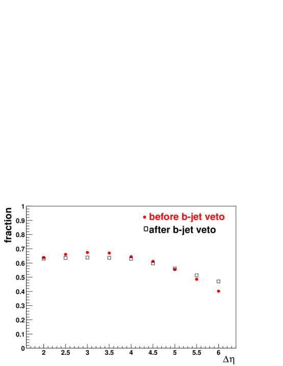
Figure 59: Fraction of events for which either the leading or the sub-leading jet is a b-jet as a function of the cut on $\Delta\eta_{j_{1}j_{2}}$ before and after the application of a b-jet veto.

In MC@NLO hard emissions are treated as in NLO calculations while soft/collinear emissions are handled by the MC simulation (HERWIG6.5 in this case) with the MC logarithmic accuracy: the $t\overline{t}$ rates are known to NLO while the parton shower part preserves unitarity. Comparisons between MC@NLO and LO event generators PYTHIA6.2 [355, 356] and HERWIG6.5 [363, 364] show that, within the MC@NLO approach, the low $P_{T}$ region is dominated by the parton shower prescription, while at higher $P_{T}$ the NLO calculation dominates predicting a significantly higher $P_{T}$ for the $t\overline{t}$ system.

PYTHIA6.2 predicts a softer $P_{T}$ distribution with strong differences in the high $P_{T}$ region ($P_{T}>100\,{\rm Ge}\kern-1.0pt{\rm V}$) with respect to the NLO prediction. It was also found that all three models give similar b-jet $P_{T}$ distribution.

The MC@NLO description of the second jet from the $t\overline{t}jj$ process was tested against a LO $t\overline{t}jj$ ME calculation using MadGraphII [365, 366] interfaced to HERWIG6.5 [367]. To reduce the double-counting in the HERWIG6.5 interface with MadGraphII, the parton shower cutoff was set to the $P_{T}$ of the lowest $P_{T}$ QCD parton in the ME calculation. The resulting $P_{T}$ distribution comparison showed that MC@NLO predicts a sub-leading non-b jet which is in good agreement for $P_{T}>50\,{\rm Ge}\kern-1.0pt{\rm V}$ with the MadGraphII $t\overline{t}jj$ ME calculation. In conclusion, MC@NLO also provides a reasonable description of the sub-leading radiation.

MC@NLO was used to define a $t\overline{t}j$ control sample via an event selection similar to the one used in [351, 352, 353, 354]. The dependence of various kinematic distributions on $\Delta\eta_{j_{1}j_{2}}$ was evaluated. In a large fraction ($\simeq 20\%$) of events with small values of $\Delta\eta_{j_{1}j_{2}}$, both leading jets are b-jets. For $\Delta\eta_{j_{1}j_{2}}>3.5$ about $65\%$ of the events have just one of the two leading jets being a b-jet (see Figure 59). This fraction is clearly dominated by $t\overline{t}j$ where the extra jet is hard. The rest of the events were examined and about $30\%$ were found to have two leading jets that are non-b-jets. These events are dominated by $t\overline{t}jj$ where the two radiated partons are hard.

The results presented here show a small dependence of the jet topology on the b-jet veto. Only the third most energetic jet is affected but the reduction of the fraction of events for which the third jet is a b-jet is nearly constant as a function of the cut on $\Delta\eta_{j_{1}j_{2}}$. According to these results, it is possible to define a control sample in the early stages of data taking with ATLAS to study properties of the $t\overline{t}$ process (for instance, normalization, central jet veto, b-jet veto). One would like to use the part of the phase space which is dominated by $t\overline{t}j$ and this is clearly the region for which the separation of the tagging jets is $\Delta\eta_{j_{1}j_{2}}\mbox{\raisebox{-1.72218pt}{$\;\stackrel{{\scriptstyle>}}{{\scriptstyle\sim}}\;$}}3.5$. For a $<10\%$ systematic error in the normalization of the $t\overline{t}j$ background about $300-500$ pb^-1 of integrated luminosity will be needed.

4.1.2 Other Background Processes

Other background processes were considered [242]:

• Electro-weak $WWjj$ production; a quark scattering process mediated by a vector boson, where the W bosons are produced and decay leptonically. This process is the second-dominant background for most masses. To model this process, we use a ME [369] that has been interfaced to PYTHIA6.1 [370].

• QCD $WWjj$ production. For this process, we use the generator provided in PYTHIA6.1.

• Electro-weak $Zjj$ production. A $Z$ boson is produced in a weak-boson-mediated quark-scattering process and decays into $\tau$’s, which in turn decay leptonically. This process was modelled using a LO ME from the MadCUP project [371].

• QCD $Zjj$ production. For this process, we use a LO ME from the MadCUP project. As before, we consider events where $Z\rightarrow\tau^{+}\tau^{-}$, $\tau\rightarrow l\nu\nu$.

• QCD $Zjj$ production with $Z\rightarrow l^{+}l^{-}$ and $l=e,\mu$. This background can be reduced substantially by requiring a minimum missing $P_{T}$. However, it cannot be ignored because of its large cross-section. We model this process with the generator provided within PYTHIA6.1.

4.2 Event Selection

Cut	VBF	$t\overline{t}$	EW $WW$	QCD $WW$	EW $Zjj$	QCD $Zjj$
a	33.2	3.34$\times 10^{3}$	18.2	670	11.6	2.15$\times 10^{3}$
b	13.1	128	11.1	3.58	3.19	66.9
c	12.4	117	10.5	3.31	1.13	19.6
d	10.1	85.1	7.74	0.95	0.96	8.55
e	7.59	13	5.78	0.69	0.90	6.01
f	5.67	2.26	1.03	0.16	0.27	0.92
g	4.62	1.12	0.44	0.1	0.01	0.02

Table 14: Cut flow for $M_{H}=160\,{\rm Ge}\kern-1.0pt{\rm V}$ in the $e-\mu$ channel. Effective cross-sections are given in fb. The event selection presented in Section 4.2 is used. MC@NLO was used to estimate the contribution from $t\overline{t}$ production (see Section 4.1.1)

Our procedure for optimizing the cuts is as follows: Begin with a set of loose (pre-selection) cuts and choose cuts on $\Delta\eta_{j_{1}j_{2}}$, $\Delta\eta_{ll}$, $\Delta\phi_{ll}$, $M_{j_{1}j_{2}}$, $M_{ll}$, and the transverse mass, $M_{T}$, that optimize $S/\sqrt{B}$, where S and B are the expected number of signal and background events for $30\,$fb^-1 of luminosity, respectively. We perform this optimization with a genetic algorithm [372]. We perform this procedure for several masses and find a parametrization for the optimal cut as a function of the Higgs mass.

The following event selection was chosen:

• Topology cuts. Require two charged leptons ($e,\mu$) that pass the single or double charged lepton trigger in ATLAS. Here, a veto on b-jets is applied (see Section 2 and [242]).

• Forward jet tagging with $P_{Tj_{1}},P_{Tj_{2}}>20\,{\rm Ge}\kern-1.0pt{\rm V}$ and $\Delta\eta_{j_{1}j_{2}}^{min}<\Delta\eta_{j_{1}j_{2}}$ according to

  $$\Delta\eta_{j_{1}j_{2}}^{min}={a\over(M_{H}-b)}+cM_{H}+d,$$ (55)

  where $a=2861$, $b=-327$, $c=9.6\times 10^{-3}$, and $d=-3.44$. Leptons are required to be in between jets in pseudorapidity.

• Tau rejection [351, 352, 353, 354, 242].

• Tagging jets invariant mass: $520\,{\rm Ge}\kern-1.0pt{\rm V}<M_{j_{1}j_{2}}<3325\,{\rm Ge}\kern-1.0pt{\rm V}$

• Central jet veto (see Section 2 and [242]).

• Lepton angular cuts: We require $\Delta\eta_{ll}<\Delta\eta_{ll}^{max}$ with

  $$\Delta\eta_{ll}^{max}=a+bM_{H}+cM_{H}^{2},$$ (56)

  where $a=6.25$, $b=-6.24\times 10^{-2}$, $c=1.99\times 10^{-4}$ for $M_{H}<200\,{\rm Ge}\kern-1.0pt{\rm V}$, and $a=3.88$, $b=-4.17\times 10^{-3}$, $c=0$ for $M_{H}>200\,{\rm Ge}\kern-1.0pt{\rm V}$. It is required that $\Delta\phi_{ll}^{min}<\Delta\phi_{ll}<\Delta\phi_{ll}^{max}$ with

  $$\Delta\phi_{ll}^{min}=a+bM_{H},$$ (57)

  where $a=-2.20$, $b=7.54\times 10^{-3}$, and

  $$\Delta\phi_{ll}^{max}=a+bM_{H}+cM_{H}^{2}+dM_{H}^{3},$$ (58)

  where $a=-4.07$, $b=0.156559$, $c=-1.310956\times 10^{-3}$, and $d=3.42011\times 10^{-6}$. As one would expect, the minimum cut is only important at high Higgs masses, and the upper bound is only relevant at low Higgs masses. It is required that $M_{ll}^{min}<M_{ll}<M_{ll}^{max}$ with

  $$M_{ll}^{min}=a(M_{H}-b)^{2}+c,$$ (59)

  where $a=-2.82\times 10^{-3}$, $b=464$, $c=129$, and

  $$M_{ll}^{max}={{a(M_{H}-b)^{2}}\over{d+(M_{H}-b)^{2}}}+c,$$ (60)

  where $a=310$, $b=114$, $c=47.6$, and $d=13290$. In order to further reduce the contribution from Drell-Yan, we require $85<M_{ll}<95\,{\rm Ge}\kern-1.0pt{\rm V}$ and $/\!\!\!p_{T}>30\,{\rm Ge}\kern-1.0pt{\rm V}$, if leptons are of same flavor.

• Transverse mass cuts. We require that $M_{T}^{min}<M_{T}<M_{T}^{max}$, with

  $$M_{T}^{min}=a+bM_{H},$$ (61)

  where $a=-17$ and $b=0.73$ and

  $$M_{T}^{max}=a+bM_{H}+cM_{H}^{2}+dM_{H}^{3},$$ (62)

  where $a=106$, $b=-0.83$, $c=9.46\times 10^{-3}$, and $d=-9.49\times 10^{-6}$. We also require $m_{T}(ll\nu\nu)>30\,{\rm Ge}\kern-1.0pt{\rm V}$, with $m_{T}(ll\nu\nu)=\sqrt{2P^{ll}_{T}/\!\!\!p_{T}(1-\cos{\Delta\phi})}$, where $P^{ll}_{T}$ is the $P_{T}$ of the di-lepton system and $\Delta\phi$ corresponds to the angle between the di-lepton vector and the $/\!\!\!p_{T}$ vector in the transverse plane.

$M_{H}({\rm Ge}\kern-1.0pt{\rm V})$	$e-\mu$	$e-e$	$\mu-\mu$	Combined
115	0.9	0.4	0.5	1.4
130	3.0	1.5	2.2	4.3
160	8.2	5.1	6.3	11.6
200	4.4	2.6	3.0	6.0
300	2.3	1.4	1.5	3.1
500	1.0	0.6	0.6	1.5

Table 15: Expected Poisson significance for the parameterized cuts listed in Section 4.2 with 10 fb^-1 of integrated luminosity. A 10% systematic uncertainty is applied to all backgrounds when calculating the significance.

4.3 Results and Discovery Potential

Table 14 displays effective cross-sections for signal and background after application of successive cuts presented in Section 4.2. Cross-sections are presented for $M_{H}=160\,{\rm Ge}\kern-1.0pt{\rm V}$ in the $e-\mu$ channel. It is worth noting that the central jet veto survival probability for $t\overline{t}$ production is significantly lower than that reported in [242]. However, this is compensated by a lower rejection due to requiring two tagging jets (see cut b in the previous Section). As a result, the relative contribution to the background from $t\overline{t}$ production obtained here is similar to the one reported in [242]. Table 15 reports the expected Poisson significance for 10 fb^-1 of integrated luminosity. Simple event counting is used and a $10\,\%$ systematic error on the background determination was assumed. In order to incorporate the systematic errors we incorporated [373, 374] the formalism developed in [375]. The implementation of MC@NLO to simulate the $t\overline{t}$ background has not changed the conclusions drawn in [242] for the $M_{H}$ considered there. The $H\rightarrow W^{(*)}W^{(*)}\rightarrow l^{+}l^{-}/\!\!\!p_{T}$ mode has a strong potential in a wide rage of Higgs masses. A significance of or greater than $5\,\sigma$ may be achieved with 30 fb^-1 of integrated luminosity for $125<M_{H}<300\,{\rm Ge}\kern-1.0pt{\rm V}$.

5 The $H\rightarrow\gamma\gamma$ Mode

5.1 Generation of Background Processes

The relevant background processes for this mode are subdivided into two major groups. Firstly, the production of two $\gamma$’s associated with two jets (real photon production). Secondly, a sizeable contribution is expected from events in which at least one jet is misidentified as a photon (fake photon production). Despite the impressive jet rejection rate after the application of $\gamma$ selection criteria expected to be achieved by the ATLAS detector [347] ($\mbox{\raisebox{-1.72218pt}{$\;\stackrel{{\scriptstyle>}}{{\scriptstyle\sim}}\;$}}10^{3}$ for each jet), the contribution from fake photons will not be negligible due to the large cross-sections of QCD processes at the LHC.

LO ME based MC’s were used to simulate $\gamma\gamma jj$ (both QCD and EW diagrams), $\gamma jjj$ and $jjjj$ production. For this purpose MadGraphII [365, 366] interfaced with PYTHIA6.2 was used [367]. The factorization and re-normalization scales were set to the $P_{T}$ of the lowest $P_{T}$ parton.

After the application of a number of basic cuts at the generator level (see [303]) the QCD and EW $\gamma jjj$ diagrams correspond to 6.32 nb and 1.21 pb, respectively. Assuming an effective jet rejection of the order of $10^{3}$, the starting cross-section for the EW $\gamma jjj$ process would be about $1\,$fb. This small cross-section will be severely reduced after the application of further selection cuts (see Section 5.2). In the analysis EW $\gamma jjj$ and $jjjj$ diagrams were neglected.

5.2 Event Selection

A number of pre-selection cuts are applied which are similar to those used in the multivariate analysis of VBF $H\rightarrow W^{(*)}W^{(*)}\rightarrow l^{+}l^{-}/\!\!\!p_{T}$ [376]:

• $P_{T\gamma 1},P_{T\gamma 2}>25\,{\rm Ge}\kern-1.0pt{\rm V}$. The $\gamma$’s are required to fall in the central region of the detector excluding the interface between the barrel and end-cap calorimeters ($1.37<\left|\eta\right|<1.52$). The latter requirement reduces the acceptance by about 10$\%$.

• Tagging jets with $P_{Tj_{1}},P_{Tj_{2}}>20\,{\rm Ge}\kern-1.0pt{\rm V}$ and $\Delta\eta_{j_{1}j_{2}}>3.5$.

• The $\gamma$’s should be in between the tagging jets in pseudorapidity.

• Invariant mass of the tagging jets, $M_{j_{1}j_{2}}>100\,{\rm Ge}\kern-1.0pt{\rm V}$.

• Central jet veto [242].

• Invariant mass window: $M_{H}-2\,{\rm Ge}\kern-1.0pt{\rm V}<M_{\gamma\gamma}<M_{H}+2\,{\rm Ge}\kern-1.0pt{\rm V}$.

The final event selection is obtained by means of maximizing the Poisson significance for 30 fb^-1 of integrated luminosity for $M_{H}=120\,{\rm Ge}\kern-1.0pt{\rm V}$. The maximization procedure is performed with the help of the MINUIT program [377]. The following variables are chosen: $P_{Tj_{1}}$, $P_{Tj_{2}}$, $\Delta\eta_{j_{1}j_{2}}$, $\Delta\phi_{j_{1}j_{2}}$, $M_{j_{1}j_{2}}$, $P_{T\gamma_{1}}$, $P_{T\gamma_{2}}$, and $\Delta\eta_{\gamma\gamma}$.

Due to the implementation of parton shower and hadronization effects, the kinematics of the final state will be somewhat different from that of the parton level analysis performed in [378]. After the application of cut f in the pre-selection, the dominant background corresponds to QCD $\gamma\gamma jj$ and the fake photon production, therefore, the optimization process will be mainly determined by the kinematics of these process together with that of the VBF signal.

Cut	Pre-selection	Parton Level	Optimization
a	$P_{T\gamma 1},P_{T\gamma 2}>25\,{\rm Ge}\kern-1.0pt{\rm V}$	$P_{T\gamma 1}>50\,{\rm Ge}\kern-1.0pt{\rm V}$	$P_{T\gamma 1}>57\,{\rm Ge}\kern-1.0pt{\rm V}$
		$P_{T\gamma 2}>25\,{\rm Ge}\kern-1.0pt{\rm V}$	$P_{T\gamma 2}>34\,{\rm Ge}\kern-1.0pt{\rm V}$
			$\Delta\eta_{\gamma\gamma}<1.58$, $\Delta\phi_{\gamma\gamma}<3$ rad
b	$P_{Tj_{1}},P_{Tj_{2}}>20\,{\rm Ge}\kern-1.0pt{\rm V}$	$P_{Tj_{1}}>40\,{\rm Ge}\kern-1.0pt{\rm V}$	$P_{Tj_{1}}>40\,{\rm Ge}\kern-1.0pt{\rm V}$
		$P_{Tj_{2}}>20\,{\rm Ge}\kern-1.0pt{\rm V}$	$P_{Tj_{2}}>29.5\,{\rm Ge}\kern-1.0pt{\rm V}$
	$\Delta\eta_{j_{1}j_{2}}>3.5$	$\Delta\eta_{j_{1}j_{2}}>4.4$	$\Delta\eta_{j_{1}j_{2}}>3.9$
d	$M_{j_{1}j_{2}}>100\,{\rm Ge}\kern-1.0pt{\rm V}$	-	$M_{j_{1}j_{2}}>610\,{\rm Ge}\kern-1.0pt{\rm V}$

Table 16: Values of the cuts applied for different event selections (see Section 5.2).

Initially, it has been verified that the inclusion of variables additional to those considered in [378] improves the signal significance. The addition of the photon related variables $\Delta\eta_{\gamma\gamma}$ and $\Delta\phi_{\gamma\gamma}$ improves the signal significance by some $10-20\%$ depending on the Higgs mass. The implementation of those two variables separately proves more efficient than the combined $\Delta R_{\gamma\gamma}$. The inclusion of the hadronic variable $\Delta\phi_{jj}$ does not noticeably increase the signal significance.

Table 16 shows the results of the optimization together with the values of the cuts placed at the pre-selection level and for the parton level analysis performed in [378]. Due to the significant increase in the background contribution compared to the parton level analysis, the optimized event selection is significantly tighter, resulting into reduced signal and background rates (see Section 5.3). The increase of the background comes from the different choice of the width of the mass window, the implementation of parton showers for the estimation of the central jet veto probability and the inclusion of fake photon events.

5.3 Results and Discovery Potential

Here, we use the event selection obtained in the optimization procedure performed in Section 5.2 (see Table 16). The expected signal and background cross-sections corrected for acceptance and efficiency corrections are shown in Table 17 for a mass window around $M_{H}=120\,{\rm Ge}\kern-1.0pt{\rm V}$ after the application of successive cuts.

The contribution from the fake photon background has been severely reduced thanks to the inclusion of the photon angular variables. The contribution from this background, however, is important. The normalization of the fake photon background is subject to sizeable systematic uncertainties. This is partly due to the uncertainty on the determination of the fake photon rejection rate [347].

Figure 60 shows the expected signal and background effective cross-section (in fb) as a function of $M_{\gamma\gamma}$ for $M_{H}=130\,{\rm Ge}\kern-1.0pt{\rm V}$. The dashed line shows the total background contribution whereas the dotted line corresponds to the real $\gamma\gamma$ background. The solid line displays the expected contribution of signal plus background.

Figure 60: Expected signal and background effective cross-section (in fb) as a function of $M_{\gamma\gamma}$ for $M_{H}=130\,{\rm Ge}\kern-1.0pt{\rm V}$. The dashed line shows the total background contribution whereas the dotted line corresponds to the real $\gamma\gamma$ background. The solid line displays the expected contribution of signal plus background.

In Table 18, results are given in terms of $S$ and $B$, for 30 fb^-1 of integrated luminosity. The signal significance was calculated with a Poissonian calculation. The signal significance expected with this VBF mode alone reaches 2.2$\,\sigma$ for 30 fb^-1 of integrated luminosity.

The QCD $\gamma\gamma jj$ has been estimated with QCD $\gamma\gamma jj$ ME based MC alone. The rate of additional (non tagging) jets has been estimated with the help of the parton shower. This approach yields a central jet veto survival probability significantly smaller than that calculated in [378]. Both effects go in the direction of overestimating of the $\gamma\gamma jj$ background. Similar discussion applies to the estimation of the fake photon background performed here. This background estimation may be improved with the implementation of a more realistic MC for the simulation of the real photon background. This mode is considerably more sensitive to the understanding of fake photon rejection than the inclusive analysis [347].

Cut	VBF H	g-g Fusion H	QCD $\gamma\gamma jj$	EW $\gamma\gamma jj$	$\gamma jjj$	$jjjj$
a	2.25	5.45	246.90	7.97	172.60	691.06
b	0.73	0.08	31.83	4.39	28.30	35.22
c	0.70	0.07	16.81	4.20	21.76	30.06
d	0.57	0.04	7.43	3.69	12.77	16.99
e	0.42	0.02	5.41	2.50	8.52	8.49
f	0.38	0.02	0.28	0.14	0.22	0.25

Table 17: Expected signal and background cross-sections (in fb) corrected for acceptance and efficiency corrections after the application of successive cuts (see Section 5.2). Here $M_{H}=120\,{\rm Ge}\kern-1.0pt{\rm V}$.

$M_{H}$	$S$	$B$	$S/B$	$\sigma_{P}$
110	10.05	30.69	0.33	1.56
120	12.06	26.54	0.45	2.02
130	12.52	23.97	0.52	2.19
140	10.91	22.90	0.48	1.94
150	7.69	20.15	0.38	1.42
160	2.89	17.21	0.17	0.44

Table 18: Expected number of signal and background events, $S/B$ and the corresponding signal significance for 30 fb^-1 of integrated luminosity (see Section 5.3).

6 The $H\rightarrow ZZ\rightarrow l^{+}l^{-}q\overline{q}$ Mode

6.1 Generation of Background Processes

Cross-section for the QCD $Z+4j,Z\rightarrow l^{+}l^{-},l=e,\mu$ process were calculated with two independent packages: ALPGEN [379] and MadGraphII [365, 366]. Both calculations include the $Z/\gamma^{\star}$ interference effects. The following cuts at the generator level were used for the cross-section calculation for the nominal event generation:

• QCD parton’s transverse momentum, $P_{T}>20\,{\rm Ge}\kern-1.0pt{\rm V}$, pseudorapidity, $\left|\eta\right|<5$. Separation between QCD partons, $\Delta R>0.5$.

• Minimal transverse momentum cuts on leptons, $P_{T}>3\,{\rm Ge}\kern-1.0pt{\rm V}$ with $\left|\eta\right|<3$. The angle separation between leptons and leptons and jets were set to $\Delta R>0.2$

The Born level cross-section of QCD $Z+4j$ production is subject to large uncertainties. Some properties of jets in association with $W$ and $Z$ bosons have been studied and have been compared with QCD predictions at the Tevatron [380, 381]. The measured cross-sections of $W/Z+n~{}jets$ where $n=1,2,3,4$ lie in between the LO predictions calculated using the re-normalization and factorization scales equal to the average transverse momentum of the partons, $\langle P_{T}\rangle$, and the transverse energy of the weak boson, $E_{T}^{WB}$, respectively. The LO prediction calculated with the first choice of scale systematically undershoots the measured cross-section. At the LHC $\langle P_{T}\rangle>100\,{\rm Ge}\kern-1.0pt{\rm V}$, due to the large phase space. Thus, the scale was set to the mass of the weak boson.

After the application of the cuts at the generator level and the choice of scales mentioned above both ALPGEN and MadGraphII yield $47.5\,$pb. 8.5 million un-weighted events were generated with MadGraphII. The output from MadGraphII was interfaced to the HERWIG6.5 package [367]. In order to avoid severe double counting in the generation of hadronic jets, the scale of the parton shower evolution was set to the $P_{T}$ of the lowest transverse momentum parton in the event.

The cross-section for $Z+4j,Z\rightarrow l^{+}l^{-},l=e,\mu$ production with one EW boson in the internal lines was evaluated with MadGraphII. These diagrams include QCD $ZZjj$ and $ZW^{\pm}jj$. A cross-section of $1.6\,$pb was obtained after cuts at generator level and by applying the same choice of scales as for the QCD $Z+4j$ case. The impact of these diagrams is small, hence, they were not included in the final results reported in Section 6.3. Diagrams with two EW bosons in the internal lines were not considered, as they are expected to be negligible.

A sample of events for $t\overline{t}$ production was used. These events were generated with the MC@NLO package (see Section 4.1).

6.2 Event Selection

The event selection presented in this Section is obtained by maximizing the signal significance for a Higgs for $M_{H}=300\,{\rm Ge}\kern-1.0pt{\rm V}$ with $30\,$fb^-1 of integrated luminosity.

Figure 61: Invariant mass of the Higgs candidates after the application of kinematic fits. The solid lines correspond to the sum of the signal (VBF $H\rightarrow ZZ\rightarrow l^{+}l^{-}q\overline{q}$) and the main background (QCD $Z+4j,Z\rightarrow l^{+}l^{-},l=e,\mu$). The dashed lines show the contribution of the main background alone. Here $M_{H}=190,200,250,300\,{\rm Ge}\kern-1.0pt{\rm V}$.

A number of basic features common to VBF modes remain. A feature specific to the mode under study is the additional ambiguity in the definition of tagging jets introduced by the presence of relatively hard jets produced from the decay of the $Z$’s. A search for two jets with an invariant mass close to $Z$ mass, $M_{Z}$, is performed. After reconstructing the $Z$ decaying hadronicaly, the event looks like a “typical” VBF candidate.

The following event selection was chosen:

• Two isolated, oppositely charged, of equal flavor leptons in the central detector region, $\left|\eta\right|<2.5$.

• The event is required to pass the single or double lepton trigger in ATLAS.

• Two hadronic jets ($j_{3},j_{4}$) with transverse momentum, $P_{T}>30\,{\rm Ge}\kern-1.0pt{\rm V}$ with $M_{j_{3}j_{4}}$ close to $M_{Z}$ were required in the fiducial region of the calorimeter, $\left|\eta\right|<4.9$. The relative invariant mass resolution of two jets is expected to be approximately $10\,\%$. The following mass window was chosen: $75<M_{j_{3}j_{4}}<101\,{\rm Ge}\kern-1.0pt{\rm V}$. These jest were “masked out” from the list of jets.

• Tagging jets with $P_{Tj_{1}}>40\,{\rm Ge}\kern-1.0pt{\rm V}$, $P_{Tj_{2}}>30\,{\rm Ge}\kern-1.0pt{\rm V}$ and $\Delta\eta_{j_{1}j_{2}}>4.4$.

• Both leptons were required to lie in between the tagging jets in pseudorapidity.

• Leptonic cuts. It was required that $M_{Z}-10<M_{ll}<M_{Z}+10\,{\rm Ge}\kern-1.0pt{\rm V}$. This cut is expected to suppress di-lepton final states with $W^{+}W^{-}\rightarrow ll\nu\nu$. It is particularly important to suppress the contribution from $t\overline{t}$ production associated with jets. No b-tagging rejection algorithms were applied in this analysis due to the large branching ratio of $Z$ decaying into heavy quarks.

• The invariant mass of the tagging jets was required to be greater than $900\,{\rm Ge}\kern-1.0pt{\rm V}$.

• Central jet veto. Extra jets with $P_{T}>20\,{\rm Ge}\kern-1.0pt{\rm V}$ are looked for in the central region of the detector ($\left|\eta\right|<3.2$). However, high $P_{T}$ quarks from the decay of one of the $Z$’s are expected to radiate hard gluons with a high probability, thus, faking hadronic jets produced prior to the decay. If $\Delta R$ between the extra jet and the jets of the Higgs candidate is larger than one unit, the event is vetoed.

• In order to further reduce the contribution from events with $W^{+}W^{-}\rightarrow ll\nu\nu$, it is required that $/\!\!\!p_{T}<30\,{\rm Ge}\kern-1.0pt{\rm V}$.

The $M_{llj_{3}j_{4}}$ spectrum could be distorted due to the ambiguity in defining tagging jets. The distortion of the $M_{llj_{3}j_{4}}$ spectrum, however, is not sizeable. Figure 61 displays the $M_{llj_{3}j_{4}}$ spectra for signal and background after the application of the event selection presented in this Section. A Higgs mass resolution of approximately $2.5\%$ is obtained for $2M_{Z}<M_{H}<300\,{\rm Ge}\kern-1.0pt{\rm V}$ [382].

6.3 Results and Discovery Potential

Table 19 shows the expected signal effective cross-sections (in fb) for a Higgs mass of $M_{H}=300\,{\rm Ge}\kern-1.0pt{\rm V}$. Table 19 also displays the effective cross-sections for the major background processes. Cross-sections are given after successive cuts (see Section 6.2). The background is largely dominated by the QCD $Z+4j,Z\rightarrow l^{+}l^{-},l=e,\mu$ production. Diagrams with one or two EW boson in the internal lines were neglected. The contribution from $t\overline{t}$ is small and it is also neglected in the final results.

Process	a	b	c	d	e	f	g	h	i
VBF ($M_{H}=300\,{\rm Ge}\kern-1.0pt{\rm V}$)	31.69	31.50	12.63	3.39	3.26	2.93	2.24	1.72	1.66
QCD $Z+4j$	25930	25902	10345	277	205	205	116	36.6	34.6
$t\overline{t}$	14793	14268	4233	135	106	10.5	6.4	2.3	0.3

Table 19: Expected effective cross-sections (in fb) for $H\rightarrow ZZ\rightarrow llq\overline{q}$ produced via VBF $(M_{H}=300\,{\rm Ge}\kern-1.0pt{\rm V}$) and the main background processes. Cross-sections are given after successive cuts presented in Section 6.2.

Table 20 reports results in terms of $S$, $B$, $S/B$ and signal significance, $\sigma_{L}$, with 30 fb^-1 of integrated luminosity for different values of $M_{H}$. The effective signal and background cross-sections are evaluated in a $4\,\sigma_{M}$ (where $\sigma_{M}$ is the mass resolution) wide mass window. The signal significance was calculated with a likelihood ratio technique using the invariant mass of the Higgs candidate as a discriminant variable [373, 374]. A signal significance of $3.75\,\sigma$ may be achieved for $M_{H}=300\,{\rm Ge}\kern-1.0pt{\rm V}$ with 30 fb^-1 of integrated luminosity. It should be noted that the cross-sections for the main background reported here are subject to large theoretical uncertainty. Fortunately, the background may be determined from side bands for Higgs searches with $M_{H}>200\,{\rm Ge}\kern-1.0pt{\rm V}$.

$M_{H}({\rm Ge}\kern-1.0pt{\rm V})$	$S$	$B$	$S/B$	$\sigma_{L}$
190	18.9	31.2	0.61	3.47
200	27.3	52.8	0.52	3.76
300	39.3	116.1	0.34	3.75
500	20.1	124.2	0.16	1.98

Table 20: Expected number of signal and background events, ratio of signal to background and signal significance (in $\sigma$) for a SM Higgs produced via VBF using the decay mode $H\rightarrow ZZ\rightarrow l^{+}l^{-}q\overline{q}$ with 30 fb^-1 of integrated luminosity for different values of $M_{H}$. The effective signal and background cross-sections are evaluated in a $4\,\sigma_{M}$ (where $\sigma_{M}$ is the mass resolution) wide mass window. The signal significance, $\sigma_{L}$, was calculated with a likelihood ratio technique using the invariant mass of the Higgs candidate as a discriminant variable.

7 Multivariate Analysis

Results reported in [242] and the present paper were based on classical cut analyses. Multivariate techniques have been extensively used in physics analyses, for instance, in LEP experiments. Neural Networks (NN) are the most commonly used tools in multivariate analyses. NN training has been performed on the $H\rightarrow W^{(*)}W^{(*)}\rightarrow l^{+}l^{-}/\!\!\!p_{T}$ [376] and $H\rightarrow\tau^{+}\tau^{-}\rightarrow l^{+}l^{-}/\!\!\!p_{T}$ [383] modes. NN training was performed with a relatively small number of variables. It was required that these variables are infra-red safe and their correlations do not depend strongly on detector effects: $\Delta\eta_{j_{1}j_{2}}$, $\Delta\phi_{j_{1}j_{2}}$, $M_{j_{1}j_{2}}$, $\Delta\eta_{ll}$, $\Delta\phi_{ll}$, $M_{ll}$, and $M_{T}$ (or the invariant mass of the $\tau^{+}\tau^{-}$ system in the case of the $H\rightarrow\tau^{+}\tau^{-}\rightarrow l^{+}l^{-}/\!\!\!p_{T}$ mode). The signal significance was calculated with a likelihood ratio technique using the NN output as a discriminant variable. An enhancement of approximately $30-50\,\%$ of the signal significance with respect to the classical cut analysis was obtained for both modes under consideration.

8 Conclusions

The discovery potential for the SM Higgs boson produced with VBF in the range $115<M_{H}<500\,{\rm Ge}\kern-1.0pt{\rm V}$ has been reported. An updated study at hadron level followed by a fast detector simulation of the $H\rightarrow W^{(*)}W^{(*)}\rightarrow l^{+}l^{-}/\!\!\!p_{T}$ mode has been presented: the main background, $t\overline{t}$ associated with jets, has been modelled with the MC@NLO program and the Higgs mass range has been extended to $500\,{\rm Ge}\kern-1.0pt{\rm V}$. This mode has a strong potential: a signal significance of more than $5\,\sigma$ may be achieved with 30 fb^-1 of integrated luminosity for $125<M_{H}<300\,{\rm Ge}\kern-1.0pt{\rm V}$. The discovery potential of the $H\rightarrow\gamma\gamma$ and $H\rightarrow ZZ\rightarrow l^{+}l^{-}q\overline{q}$ modes have also been reported with analyses at hadron level followed by a fast detector simulation.

The discovery potential of the modes presented in this work was combined with results reported in past studies performed for the ATLAS detector. Results from recent studies [384, 309, 385], which were not used in [242], were added here. Likelihood ratio techniques have been used to perform the combination [373, 374]. In order to incorporate systematic errors, the formalism developed in [375] was implemented. A 10 % systematic error on the background estimation has been assumed for modes related to VBF [242]. Figure 62 displays the overall discovery potential of the ATLAS detector with 10 fb^-1 of integrated luminosity. Results from NN based analyses and discriminating variables have not been included in the combination. The present study confirms the results reported in [351, 352, 353, 354, 242], that the VBF mechanism yields a strong discovery potential at the LHC in a wide range of the Higgs boson mass.

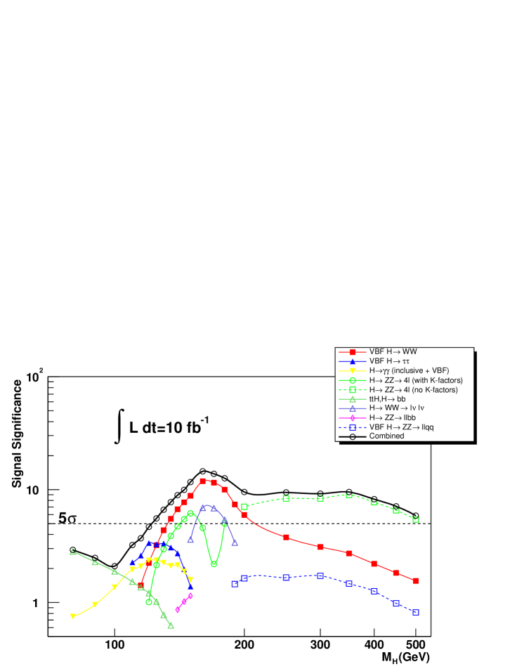
Figure 62: Expected significance for ATLAS as a function of Higgs mass for 10 fb^-1 of integrated luminosity.

F. Four-Lepton Signatures at the LHC of heavy neutral MSSM Higgs Bosons via Decays into Neutralino/Chargino Pairs
M. Bisset, N. Kersting, J. Li, S. Moretti and F. Moortgat

1 Introduction

There have been four previous studies [386, 387, 388, 389] focusing on the discovery potential of the decays of the heavier neutral MSSM Higgs bosons into neutralinos and charginos (henceforth, –inos):

$$H^{0},A^{0}\rightarrow\tilde{\chi}_{a}^{+}\tilde{\chi}_{b}^{-},\tilde{\chi}_{i}^{0}\tilde{\chi}_{j}^{0}\;\;\;\;\;\;\;(a,b=1,2,\;\;i,j=1,2,3,4).$$ (63)

However, all such works dealt only with the channels $H^{0},A^{0}\rightarrow\tilde{\chi}_{2}^{0}\tilde{\chi}_{2}^{0}$. Furthermore, the subsequent neutralino decays $\tilde{\chi}_{2}^{0}\rightarrow\tilde{\chi}_{1}^{0}\ell^{+}\ell^{-}$ ($\ell=e$ or $\mu$) were always assumed to proceed via three-body decays with an off-shell intermediate $Z^{0*}$ or slepton, neglecting the possibility of the intermediate slepton being on-mass-shell. The novelty of the present analysis is that we incorporate all the decays in (63) and allow for intermediate sleptons to be on mass-shell.

The importance of investigating the potential of SUSY decays of Higgs bosons in covering the so-called LHC wedge region of the MSSM parameter space ($4~{}\raisebox{-1.00006pt}{$\buildrel\scriptscriptstyle<\over{\scriptscriptstyle\sim}$}~{}\tan\beta~{}\raisebox{-1.00006pt}{$\buildrel\scriptscriptstyle<\over{\scriptscriptstyle\sim}$}~{}10$ and $M_{A^{0}}\raisebox{-1.00006pt}{$\buildrel\scriptscriptstyle>\over{\scriptscriptstyle\sim}$}~{}200$ GeV) – where only the lightest MSSM Higgs boson $h^{0}$ can be detected and this is indistinguishable from the Standard Model (SM) state (decoupling regime) – has already been stated in several papers, for the case of both neutral [388] and charged [390, 391, 392, 393, 62] Higgs states. The reason is twofold. Firstly, for consistency: it is rather unnatural in the MSSM to assume a heavy SUSY particle (or sparticle) spectrum as implied by only considering decays of MSSM Higgs bosons into (visible) ordinary matter, when the mechanism of Electro-Weak Symmetry Breaking (EWSB) does require sparticle masses to be at or below the TeV scale. Secondly, for the benefits: several Higgs $\to$ SUSY signals are indeed detectable at the LHC and provide the means of distinguishing the SM from the MSSM Higgs sector in the wedge region even independently of the discovery of the SUSY particles themselves in other channels [388], [390, 391, 392, 393, 62]. The rationale for looking at leptonic signatures ($\ell=e,\mu$) is clearly the difficult LHC environment (due to the large QCD activity). Finally, the reason for including Higgs decays to the heavier –inos is to extend the reach to larger Higgs masses.

It is also worthwhile to investigate the role played by sleptons, by allowing the latter to participate in the decays as both on- and off-mass-shell objects with ‘optimal’ masses, hence maximising the leptonic –ino Branching Ratios (BRs). That is, sleptons are here made as light as possible, compatibly with LEP2 [394] limits (i.e., $m_{{\tilde{e}_{1}}({\tilde{\mu}_{1}})[{\tilde{\tau}_{1}}]}\geq 99(91)[85]\,\hbox{GeV}$ and $m_{\tilde{\nu}}\geq 43.7\,\hbox{GeV}$, assuming that no slepton is nearly-degenerate with the LSP, i.e., the lightest neutralino, $\tilde{\chi}_{1}^{0}$). Flavour-diagonal inputs are adopted from the slepton sector for both the left/right soft slepton masses (selectrons, smuons and staus) and the trilinear ‘$A$-terms’. (Also notice that we adopt $m_{\tilde{e}_{R}}\simeq m_{\tilde{\mu}_{R}}$ and $m_{\tilde{e}_{L}}\simeq m_{\tilde{\mu}_{L}}$). If all three generations have the same soft inputs (with $A_{\ell}=0$, including $A_{\tau}$), then the slepton sector is effectively reduced to one optimal input value (which we identify with $m_{\tilde{\ell}_{\scriptscriptstyle R}}\equiv m_{\tilde{\ell}}$). However, since –ino decays to tau-leptons are generally not anywhere near as beneficial as are –ino decays to electrons or muons, it would be even better if the stau inputs were significantly above those of the first two generations, which reflects our approach here (we set the soft stau mass inputs $100\,\hbox{GeV}$ above those of the other sleptons). Unless stated otherwise, we take $m_{\tilde{\ell}}=$ 150 GeV ($\ell=e,\mu$), hence $m_{\tilde{\tau}}=$ 250 GeV, throughout.

2 MSSM Parameter Space

Figure 63: $\sigma(pp\rightarrow A^{0},H^{0})$ $\times$ BR$(A^{0}/H^{0}\rightarrow 4\ell N)$ (in fb), where $\ell=e^{\pm}$ or ${\mu}^{\pm}$ and $N$ represents invisible final state particles: $M_{2}=200$ GeV, $\mu=-200\,\hbox{GeV}$ with optimised slepton masses, plus $m_{t}=175\,\hbox{GeV}$, $m_{b}=4.25\,\hbox{GeV}$, $m_{\tilde{q}}=1\,\hbox{TeV}$, $m_{\tilde{g}}=800\,\hbox{GeV}$ and $A_{\ell}=0$.

The total event rate for all possible four-lepton channels is found in Fig. 63, over the customary $(M_{A^{0}},\tan\beta)$ plane, for the representative choice of SUSY parameters $M_{2}=200$ GeV ($M_{1}=\frac{5}{3}\tan^{2}\theta_{W}M_{2}$) and $\mu=-200$ GeV (and optimal slepton masses as defined above). The normalisation of the $gg\to H^{0}/A^{0}$ and $gg,q\bar{q}\to b\bar{b}H^{0}/A^{0}$ production channels is from the SUSY implementation [296] of HERWIG [294] in v6.4 [395] default configuration – except for the choice of CTEQ6L Parton Distribution Functions (PDFs) – whereas decay rates are extracted from ISASUSY/ISASUGRA routines [396] interfaced to HERWIG via the ISAWIG module [397]. While the maximum of the cross section is found at $M_{A^{0}}\approx 300$ to 400 GeV for large $\tan\beta$, in the critical wedge region the production and decay rates are still favourable, ranging from 500 to 5000 four-lepton events per year at high luminosity (before any cuts).

The plots in Fig. 64 show the event rates in the plane $(M_{2},\mu)$ for a choice in $\tan\beta$, equal to 8, and a selection of $M_{A^{0}}$ values (400, 500 and 600 GeV) in the core of the wedge region. The distribution of decay rates as highlighted by the colour scheme proves that the main source of the four-lepton signals emerging from the decays in (63) at such optimal points in the SUSY parameter space shifts from $\tilde{\chi}_{2}^{0}\tilde{\chi}_{2}^{0}$ to heavier –ino pairs as $M_{A^{0}}$ rises from ${\raisebox{-1.00006pt}{$\buildrel\scriptscriptstyle<\over{\scriptscriptstyle\sim}$}}~{}400~{}\hbox{GeV}$ to ${\raisebox{-1.00006pt}{$\buildrel\scriptscriptstyle<\over{\scriptscriptstyle\sim}$}}~{}600~{}\hbox{GeV}$. Also, a new region of the –ino parameter space is opened up: the $\tilde{\chi}_{2}^{0}\tilde{\chi}_{2}^{0}$ decays favour moderate to high $|\mu|$ and low $M_{2}$ whereas the decays to heavier –inos prefer lower $|\mu|$ values and extend up to fairly high values of $M_{2}$.

Figure 64: $\sigma(pp\rightarrow A^{0},H^{0})$ $\times$ BR$(A^{0}/H^{0}\rightarrow 4\ell N)$ (in fb), where $\ell=e^{\pm}$ or ${\mu}^{\pm}$ and $N$ represents invisible final state particles: percentage from $A^{0},H^{0}\rightarrow\tilde{\chi}^{0}_{2}\tilde{\chi}^{0}_{2}$ $>$ 90% (red), 50% – 90% (yellow), 10% – 50% (light blue), $<$ 10% (white). Parameters are: $\tan\beta=8$, $M_{A^{0}}=400\,\hbox{GeV}$ (top), $500\,\hbox{GeV}$ (middle), $600\,\hbox{GeV}$ (bottom). Optimised slepton masses are assumed, plus $m_{t}=175\,\hbox{GeV}$, $m_{b}=4.25\,\hbox{GeV}$, $m_{\tilde{q}}=1\,\hbox{TeV}$, $m_{\tilde{g}}=800\,\hbox{GeV}$ and $A_{\ell}=0$. The black shaded areas are excluded by LEP.

3 Detector Simulation Analysis

The MC used for the LHC analysis is again HERWIG v6.4 in the configuration described in the previous section. The detector simulation assumes a typical LHC experiment, as provided by private programs checked against results in literature. The event selection criteria used in the analysis are as follows.

• $4\ell$ events: we select exactly four leptons ($\ell=e$ or $\mu$) detected within $|\eta^{\ell}|<2.4$ and with initial thresholds at $E_{T}^{\ell}>7,4$ GeV for $e,\mu$, respectively. Leptons are isolated by requiring no tracks (of charged particles) with $p_{T}>1.5$ GeV in a cone of 0.3 radians around the lepton direction.

• $Z$-veto: no opposite-charge same-flavour lepton pairs may reconstruct $M_{Z}\pm 10$ GeV.

• $E_{T}^{\ell}$: all leptons must finally have $20~{}{\rm{GeV}}<E_{T}^{\ell}<80$ GeV.

• $E_{T}^{\rm{miss}}$: events must have $20~{}{\rm{GeV}}<E_{T}^{\rm{miss}}<130$ GeV (in missing transverse momentum).

• $E_{T}^{\rm{jet}}$: all jets must have $E_{T}^{\rm{jet}}<50$ GeV.

• $4\ell$ inv. m.: the four-lepton invariant mass must be $\leq M_{H^{0}}-2M_{{\tilde{\chi}}^{0}_{1}}=360$ GeV.

We have chosen two representative points for the MSSM parameter space (recall that $A_{\ell}=0$):

1. $M_{A^{0}}$ = 600 GeV, $\tan\beta$ = 10, $M_{1}$ = 125 GeV, $M_{2}$ = 250 GeV, $\mu$ = + 450 GeV, $m_{\tilde{\ell}/\tilde{\tau}}$ = 150/250 GeV, $m_{\tilde{q}/\tilde{g}}$ = 1000/800 GeV. This is a configuration in which ${\tilde{\chi}}_{2}^{0}{\tilde{\chi}}_{2}^{0}$ decays are dominant (basically 100%).

2. $M_{A^{0}}$ = 400 GeV, $\tan\beta$ = 5, $M_{1}$ = 100 GeV, $M_{2}$ = 200 GeV, $\mu=-150$ GeV, $m_{\tilde{\ell}/\tilde{\tau}}$ = 150/250 GeV, $m_{\tilde{q}/\tilde{g}}$ = 1000/800 GeV. This is a configuration in which ${\tilde{\chi}}_{2}^{0}{\tilde{\chi}}_{2}^{0}$ (50%) and ${\tilde{\chi}}_{2}^{0}{\tilde{\chi}}_{4}^{0}$ (38%) decays have comparable rates.

The relevant -ino masses can be found in Tab. 21 (recall that $M_{H^{0}}\approx M_{A^{0}}$).

Table 21: -ino masses (in GeV) for points 1.–2.

	1.	2.
${\tilde{\chi}}^{0}_{1}$	$123$	$94$
${\tilde{\chi}}^{0}_{2}$	$236$	$137$
${\tilde{\chi}}^{0}_{3}$	$455$	$167$
${\tilde{\chi}}^{0}_{4}$	$471$	$237$
${\tilde{\chi}}^{\pm}_{1}$	$236$	$136$
${\tilde{\chi}}^{\pm}_{2}$	$471$	$238$

The results of our simulations are presented in Tabs. 22–23. Despite our studies being preliminary, in the sense that a full simulation of the $t\bar{t}$ and $\tilde{t}\tilde{t}^{*}$ backgrounds is still lacking, prospects of detecting $H^{0},A^{0}$ signatures at the LHC via the decays in (63) in the interesting wedge (or decoupling) region of the MSSM seem very good. This applies not only to the already investigated ${\tilde{\chi}}_{2}^{0}{\tilde{\chi}}_{2}^{0}$ modes (point 1.), but especially to the additional ones (exemplified by the ${\tilde{\chi}}_{2}^{0}{\tilde{\chi}}_{4}^{0}$ contribution in 2.). As for the $t\bar{t}$ and $\tilde{t}\tilde{t}^{*}$ noises, we would expect these not to undermine such conclusions, based on preliminary estimates for the efficiency of extracting $4\ell$ events from top-antitop (also appearing from stop-antistop) decays. Another aspect to be mentioned is the somewhat poor efficiency for the signal following the $Z$-veto and $E_{T}^{\ell}$ cuts, particularly for point 1. However, notice that both such (or similar) requirements are needed: the former to reject the $ZZ$-noise and the second against the squark/gluino background. Some optimisation is in order in this case, though.

Table 22: Number of events after the successive cuts defined in the text for point 1. (at 100 fb^-1).

Process	$4\ell$ events	$Z$-veto	$E_{T}^{\ell}$	$E_{T}^{\rm{miss}}$	$E_{T}^{\rm{jet}}$	$4\ell$ inv. m.
$\tilde{q},\tilde{g}$	1218	417	76	14	0	0
$\tilde{\ell}$,$\tilde{\nu}$	1	0.2	0	0	0	0
$\tilde{\chi}\tilde{\chi}$	240	67	12	4	3	1
$tH^{-}$ + c.c.	1	0	0	0	0	0
$ZZ$	807	16	10	2	1	1
$ttZ$	46	1	0	0	0	0
$tth^{0}$	3	1	1	0	0	0
$A^{0},H^{0}$ signal	218(141+77)	81	29	24	20	14

Table 23: Number of events after the successive cuts defined in the text for point 2. (at 100 fb^-1).

Process	$4\ell$ events	$Z$-veto	$E_{T}^{\ell}$	$E_{T}^{\rm{miss}}$	$E_{T}^{\rm{jet}}$	$4\ell$ inv. m.
$\tilde{q}$, $\tilde{g}$	547	203	55	4	0	0
$\tilde{\ell}$,$\tilde{\nu}$	246	183	125	107	83	83
$\tilde{\chi}\tilde{\chi}$	304	123	79	66	50	48
$tH^{-}$ + c.c.	31	10	7	6	3	2
$ZZ$	1490	32	25	5	4	4
$ttZ$	49	2	0	0	0	0
$tth^{0}$	6	1	1	1	0	0
$H^{0},A^{0}$ signal	147(68+79)	98	85	68	54	54

Finally, we should mention that further studies are in progress, attempting to distinguish between ‘hadronically quiet’ vs. ‘hadronically active’ events, in the hope of further increasing the signal-to-background rates and the statistical significances of the signals. In fact, recall that the signal is produced via $gg\to H^{0}/A^{0}$ and $gg,q\bar{q}\to b\bar{b}H^{0}/A^{0}$. The former tend to produce additional jets which are rather forward and soft, so that they tend to not enter the detector. In the latter, the $b$-jets are somewhat harder, yet most of them will be missed by the apparata. Hence, it may be worthwhile to veto jet activity above $E_{T}$ values even lower than 50 GeV, as it is likely that jets from the background will populate the high $E_{T}$ region of the detector more often than those of the signal.

4 Outlook

Future work will develop along the two following directions.

1. Discovery regions Just like it was done in Refs. [388] and [391] (see also [398]), the next step of the analysis will be to express the discovery potential of the four-lepton mode over the customary $(M_{A^{0}},\tan\beta)$ plane, corresponding to some sample choices of SUSY parameters. Indeed, we foresee that a significant part of the LHC wedge region will be covered, as our results may be considered as un upgrade of those in [388, 398] (e.g., see Fig. 19(27) in [388]([398])).

2. -ino mass spectrum and -ino-ino-Higgs coupling determination This is a new direction that was not exploited in Refs. [388] and [391], so that we document it below in some detail, also showing several preliminary results. In short, the idea is to ascertain information about the gaugino mass spectrum and the Higgs-gaugino coupling strengths from a subset of our four-lepton events, limited to those with two $e^{\pm}$’s and two ${\mu}^{\pm}$’s, out of a signal enriched sample (or possibly after the SM and SUSY backgrounds have been subtracted) obtained via our selection procedure. The original idea is due to Refs. [386, 387, 388], where it was however applied to $H^{0},A^{0}\rightarrow\tilde{\chi}_{2}^{0}\tilde{\chi}_{2}^{0}$ only. Chief differences in our context are: (i) additional pairs of unlike neutralinos leading to the four-lepton events; (ii) a mixture of different gaugino pairs (charged or neutral) yielding the same multi-lepton signature; (iii) a cascade of decays leading from the original –inos generated in the Higgs boson decays to the final four-lepton (plus LSP’s) final states; (iv) the potential of many more signal events (especially at higher values of $\tan\beta$) than were anticipated in those analyses; (v) generally stiffer lepton momenta since heavier Higgs decaying into heavier –inos occur with non-negligible probability.

By making ‘Dalitz-type’ plots of various combinations of leptons’ invariant masses, we noticed some interesting structure. Consider point 2. and plot the di-lepton invariant masses $M_{e^{+}e^{-}}$ and $M_{\mu^{+}\mu^{-}}$ from the same event against each other, for the signal and the dominant SUSY backgrounds (see Tab. 22). Clearly the two-dimensional topology of the plots contains kinematical information that should point to the underlying decay. For example, one should see the ${\tilde{\chi}}^{0}_{2,4}-{\tilde{\chi}}^{0}_{1}$ mass differences from the edges of the mass distributions. (The forthcoming plots will correspond to $H^{0}+A^{0}$ signal events and assume up to $1200$ fb^-1, i.e., both ATLAS and CMS statistics after six years of LHC running at high luminosity). Fig. 65 (left plot), even if one only enforces the first two cuts (‘$4\ell$ events’ and ‘$Z$-veto’), confirms these expectations and also proves that backgrounds do not seem to alter tragically the pattern expected in the di-lepton invariant mass plots for the signal. In fact, to implement the next cut (‘$E_{T}^{\ell}$’) leads to the backgrounds fortifying the pattern expected from the signal alone, see Fig. 65 (right plot). The study of this kind of plots should enable us not only to say which decays are happening but also to extract the relevant masses and couplings entering the channels in (63). Work is in progress in this direction.

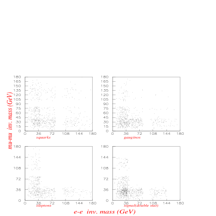
Figure 65: Left: Di-lepton invariant mass plots for the most significant backgrounds and signal corresponding to point 2., at $600$ fb^-1 (except the signal, which is twice this). Here the only cuts made are the ‘$4\ell$ events’ and ‘$Z$-veto’ ones. Right: Same as previous plot, but in presence of the additional ‘$E_{T}^{\ell}$’ cut.

5 Conclusions

We have reported on work currently being done into furthering the scope of Higgs $\to$ SUSY particle decays in the LHC quest for MSSM Higgs bosons. In particular, we have highlighted the potential of $H^{0}/A^{0}$ decays into all possible -ino pairs (both neutral and charged), finally yielding four-lepton signatures of electron and muons (plus missing energy and some hadronic activity), in covering part of the so-called wedge region of the $(M_{A^{0}},\tan\beta)$ plane expected at the LHC, where – so long that only Higgs decays into ordinary SM objects are considered – the lightest MSSM Higgs boson is the only accessible Higgs state and indistinguishable from the SM one (the so-called decoupling scenario). Our analysis expands upon previous ones [386, 387, 388, 389] which were limited to $H^{0}/A^{0}\rightarrow\tilde{\chi}_{2}^{0}\tilde{\chi}_{2}^{0}$ decays. Our conclusions of course assume that the relevant SUSY parameters are in favourable configurations, yet the latter are found to be those that will be probed first by the LHC (as they lay close to current experimental limits, see Fig. 64), so that our analysis is of immediate phenomenological impact at the CERN machine. Refinements of this work are in progress and possible outlooks in this respect were described in some detail.

G. The $H\to\gamma\gamma$ in associated Production Channel
O. Ravat and M. Lethuillier

1 Introduction

The observation of a light Higgs boson decaying to two photons in the inclusive channel is not an easy task. QCD backgrounds are important and are very demanding on ECAL performances. In this paper will be considered the $pp\to\gamma\gamma+lepton(s)$ channel. In this channel the cross section is much smaller but the strong background suppression makes a discovery less demanding on the ECAL. Another interesting feature of this channel is the presence of at least one charged lepton giving the location of the Higgs production vertex easily, with a good precision, and hence could improve the resolution on $M_{Higgs}$. Finally, it has been shown in [399] that the $\gamma\gamma+leptons$ channel could be a rescue channel in case of maximal stop mixing. In this paper will be presented the simulation tools for the generation of the events, the K-factors obtained, and the discovery potential for the $\gamma\gamma+l+E_{T_{Mis}}$ and $\gamma\gamma l^{+}+l^{-}$ final states.

2 Simulation tools

The calculation of cross sections is done using the V2HV program [400], which performs NLO calculations. The K-factors are extracted and applied to the cross-section given by the Leading Order generator : CompHEP [285]. The 4-vectors generation is done with the CompHEP package, wich allows to calculate squared matrix elements corresponding to the complete set of SM tree level diagrams of the considered processes, and performs the convolution with the parton distributions. The branching ratios concerning the Higgs decay are taken from HDECAY [165].The final state is then processed by Pythia [203, 277], which performs the hadronization and the fragmentation of the jets. Pythia is also used for the generation of underlying events and minimum-bias events. The fast detector simulation is done with CMSJET [402]

3 WH production

The Next to Leading Order calculations program V2HV gives the cross sections. CompHEP, a LO generator at the parton level, gives 1.33 times less and a K factor of 1.33 is applied for the signal. WH samples have been generated for Higgs Bosons masses from 115 GeV to 150 GeV. As no NLO generator for the background is available yet, the same factor is used for irreducible background.

4 ZH production

Again V2HV is used to determine the cross sections of the process, from $M_{H}$=115 GeV to $M_{H}$ =150 GeV. CompHEP is also used, and the K-factor is 1.27.

5 Backgrounds

For the generation of the backgrounds, only CompHEP is used. The $\gamma\gamma+l+E_{T_{Miss}}$ and $\gamma\gamma+l^{+}l^{-}$ final states are considered. The irreducible backgrounds are not taken into account yet, but according to [401] they shouldn’t be important. In order to have an efficient production, kinematical cuts were applied : both photons are required to have $p_{T}>$ 20 GeV, as well as leptons. An isolation criterium is imposed between generated particles: they have to be separated by a cone of $\Delta R=\sqrt{\Delta\phi^{2}+\Delta y^{2}}>0.3$. Finally there is a cut on the rapidity of the particles : $|y|<2.7$. The same cuts are applied to the signal and the following cross sections are found :

The cuts applied at generation don’t represent a serious handicap, as the thresholds for the Level-2 trigger are 31 GeV and 16.9 GeV GeV for di-photons, or di-electrons (12GeV for di-muons) : see [403].

6 CMSJET parametrisation

The processing of 4-vectors is done with CMSJET, a fast simulation tool. The pile-up is included at this level of the simulation, the average number of envents per bunch crossing is 17.3. Only particles satisfying the following cuts are processed by CMSJET : The minimum transverse momentum values required are the same as the ones from CompHEP. An isolation criterium is applied on photons and leptons. No charged track with $p_{T}>2$ GeV in a cone of $\Delta R=\sqrt{\Delta\phi^{2}+\Delta\eta^{2}}=0.3$ ( tracker isolation ), no cluster with more than 5 GeV in the same cone ( calorimeter isolation ). The $\eta$ cut is harder, the particles are asked to have $|\eta|<2.4$. Electronic noise is set to 50 MeV in the ECAL Barrel, 150 MeV in the endcaps. It is assumed that 0.5$\%$ of the calorimeter cells are dead. Trigger efficiencies are taken from the Data Acquisition $\&$ High Level Trigger TDR : 59$\%$ for electrons from Ws, 83.7$\%$ for the Higgs photons, and 42$\%$ for muons from Ws; We hence get a trigger efficiency of 93.32$\%$ for the $e^{\pm}\nu\gamma\gamma$ channel, and 90.55$\%$ for the $\mu^{\pm}\nu\gamma\gamma$ one.

7 Results after 1 year at high luminosity

As only irreducible backgrounds are considered in this study, a simple first analysis is used. Simple cuts on transverse momentum are applied.

The figure 66 shows $s/\sqrt{b}$ as a function of the cut on the photons momentum. We first seek the best value in terms of $s/\sqrt{b}$ for the hardest photon. Then the best cut found is applied, and the cut on the soft photon is looked for. The best set of cut is the following : 55 GeV for the hardest photon, 30 for the softest.

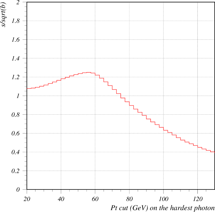
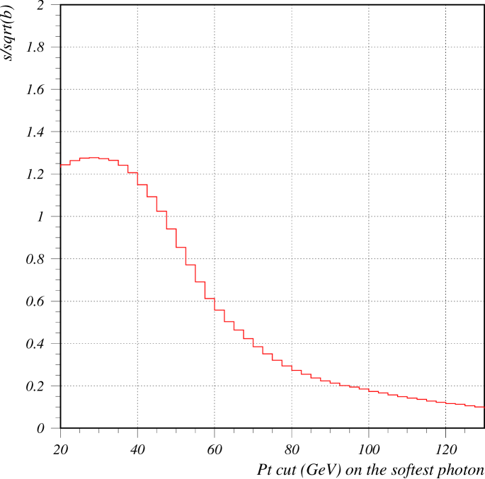
Figure 66: Choice of the cut on the hardest photon.

After simple cuts on photons of 55 GeV and 30 GeV we get the following number of events in a mass window of $M_{H}\pm 1.6GeV$ (ie : $M_{H}\pm 2\sigma$) : 13 for signal and 1.4 for background in the WH case, 1.13 and 1.73 in the ZH case.

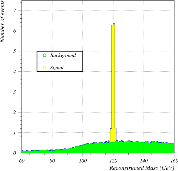
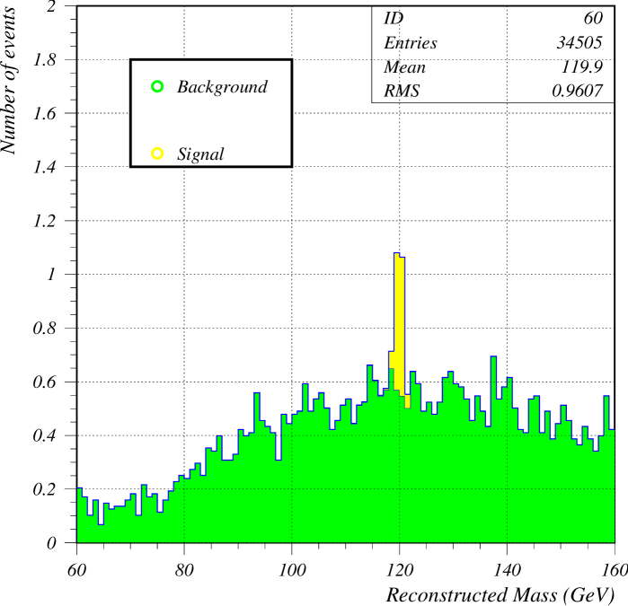
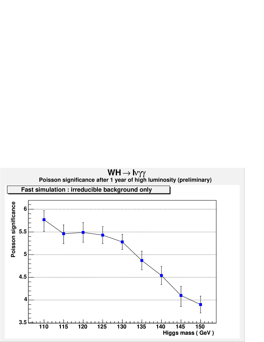
Figure 67: $M_{\gamma\gamma}$ for both channels.

Those numbers being definitely not compatible with gaussian distributions, Poisson significances have been calculated. Results are given in figure 67.

8 Conclusions and Outlook

The associated production of Higgs Bosons together with gauge bosons, despite its small cross section, looks as an interesting way of completing a discovery scheme. It is less demanding on calorimeter performances and provides easily the Higgs vertex, improving the mass resolution. This first analysis considered the feasibility of a study of this channel. Only irreducible background has been considered. The promising results from fast simulation lead us to start a complete study, using full simulation of the detector. Besides these considerations, many models beyond the Standard Model show an enhancement of the discovery potential of this channel, and will be soon studied .

H. MSSM Higgs Bosons in the Intense-Coupling Regime at the LHC
E. Boos, A. Djouadi and A. Nikitenko

1 The Intense-Coupling Regime

In the MSSM Higgs sector, the intense-coupling regime [404, 405] is characterized by a rather large value of $\tan\beta$, and a pseudoscalar Higgs boson mass that is close to the maximal (minimal) value of the CP-even $h$ ($H$) boson mass, $M_{A}\sim M_{h}^{\rm max}$, almost leading to a mass degeneracy of the neutral Higgs particles, $M_{h}\sim M_{A}\sim M_{H}$. In the following, we will summarize the main features of this scenario. For the numerical illustration, we will use HDECAY [165], fix the parameter $\tan\beta$ to the value $\tan\beta=30$ and choose the maximal mixing scenario, where the trilinear Higgs–stop coupling is given by $A_{t}\simeq\sqrt{6}M_{S}$ with the common stop masses fixed to $M_{S}=1$ TeV; the other SUSY parameter will play only a minor role.

Figure 68 (left) displays the masses of the MSSM Higgs bosons as a function of $M_{A}$. As can be seen, for $M_{A}$ close to the maximal $h$ boson mass, which in this case is $M_{h}^{\rm max}\simeq 130$ GeV, the mass differences $M_{A}-M_{h}$ and $M_{H}-M_{A}$ are less than about 5 GeV. The $H^{\pm}$ boson mass, given by $M_{H^{\pm}}^{2}\sim M_{A}^{2}+M_{W}^{2}$, is larger : in the range $M_{A}\raisebox{-3.69899pt}{~{}\shortstack{$<$ \\ [-0.07cm] $\sim$}}~{}140$ GeV, one has $M_{H^{\pm}}\raisebox{-3.69899pt}{~{}\shortstack{$<$ \\ [-0.07cm] $\sim$}}~{}160$ GeV, implying that charged Higgs bosons can always be produced in top-quark decays, $t\to H^{+}b$. The couplings of the CP-even Higgs bosons to fermions and gauge bosons normalized to the SM Higgs boson couplings are also shown in Fig. 68 (right). For small $M_{A}$ values, the $H$ boson has almost SM couplings, while the couplings of the $h$ boson to $W,Z,t$ $(b)$ are suppressed (enhanced); for large $M_{A}$ values the roles of $h$ and $H$ are interchanged. For medium values, $M_{A}\sim M_{h}^{\rm max}$, the couplings of both $h$ and $H$ to gauge bosons $V=W,Z$ and top quarks are suppressed, while the couplings to $b$ quarks are strongly enhanced. The normalized couplings of the CP-even Higgs particle are simply $g_{AVV}=0$ and $g_{Abb}=1/g_{Att}=\tan\beta=30$.

These couplings determine the branching ratios of the Higgs particle, which are shown in Fig. 69. Because the enhanced couplings, the three Higgs particle branching ratios to $b\bar{b}$ and $\tau^{+}\tau^{-}$ are the dominant ones, with values $\sim 90$% and $\sim 10$% respectively. The decays $H\to WW^{*}$ do not exceed the level of 10%, even for small $M_{A}$ values [where $H$ is almost SM-like] and in most of the $M_{A}$ range the decays $H,h\to WW^{*}$ are suppressed to the level where they are not useful. The decays into $ZZ^{*}$ are one order of magnitude smaller and the decays into $\gamma\gamma$ are very strongly suppressed for the three Higgsses and cannot be used anymore. Finally, note that the branching ratios for the decays into muons, $\Phi\to\mu^{+}\mu^{-}$, are constant in the entire $M_{A}$ range exhibited, at the level of $3\times 10^{-4}$.

Summing up the partial widths for all decays, the total decay widths of the three Higgs particles are shown in the left-hand side of Fig. 70. As can be seen, for $M_{A}\sim 130$ GeV, they are at the level of 1–2 GeV, i.e. two orders of magnitude larger than the width of the SM Higgs boson for this value of $\tan\beta$ [the total width increases as $\tan^{2}\beta$]. The right-hand side of the figure shows the mass bands $M_{\Phi}\pm\Gamma_{\Phi}$ and, as can be seen, for the above value of $M_{A}$, the three Higgs boson masses are overlapping.

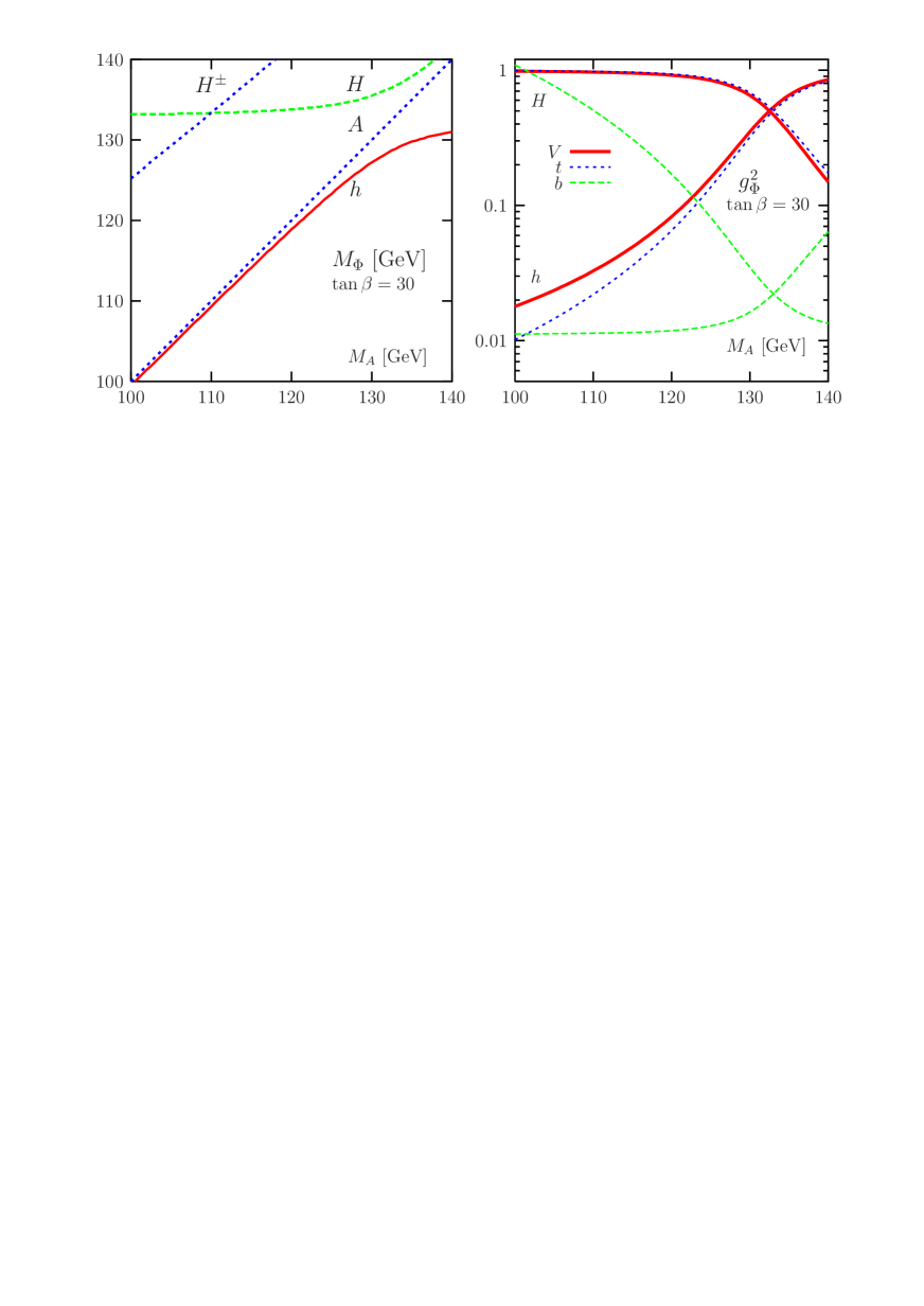
Figure 68: The masses of the MSSM Higgs bosons (left) and the normalized couplings of the CP-even Higgs bosons to vector bosons and third-generation quarks (right) as a function of $M_{A}$ and $tan\beta=30$. For the $b$-quark couplings, the values $10\times g_{\Phi bb}^{-2}$ are plotted.

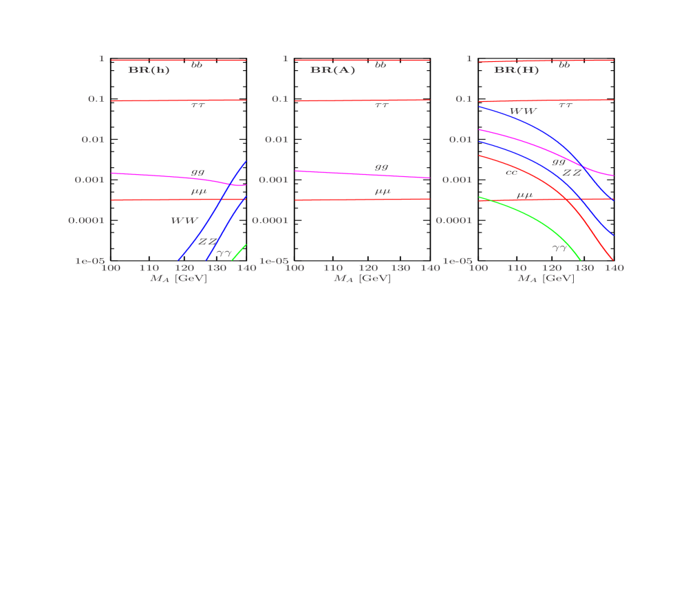
Figure 69: The branching ratios of the neutral MSSM Higgs bosons $h,A,H$ for the various decay modes as a function of $M_{A}$ and for $tan\beta=30$.

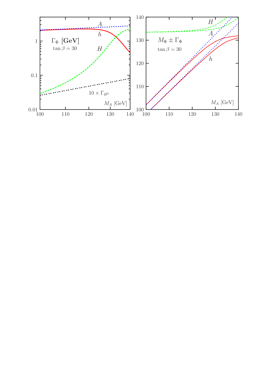
Figure 70: Total decay widths $\Gamma_{\Phi}$ (left) and the mass bands $M_{\Phi}\pm\Gamma_{\Phi}$ (right) for the neutral MSSM Higgs bosons as a function of $M_{A}$ and for $tan\beta=30$.

2 Discrimination of the three Higgs Bosons at the LHC

The most difficult problem we must face in the intense-coupling regime, is to resolve between the three peaks of the neutral Higgs bosons when their masses are close to one another. The only decays with large branching ratios on which we can rely are the $b\bar{b}$ and $\tau^{+}\tau^{-}$ modes. At the LHC, the former has too large QCD background to be useful, while for the latter channel [which has been shown to be viable for discovery] the expected experimental resolution on the invariant mass of the $\tau^{+}\tau^{-}$ system is of the order of 10 to 20 GeV, and thus clearly too large. One would then simply observe a relatively wide resonance corresponding to $A$ and $h$ and/or $H$ production. Since the branching ratios of the decays into $\gamma\gamma$ and $ZZ^{*}\to 4\ell$ are too small, a way out is to use the Higgs decays into muon pairs: although the branchings ratio is rather small, BR($\Phi\to\mu^{+}\mu^{-})\sim 3.3\times 10^{-4}$, the resolution is expected to be as good as 1 GeV, i.e. comparable to the total width, for $M_{\Phi}\sim 130$ GeV.

Because of the strong enhancement of the Higgs couplings to bottom quarks, the three Higgs bosons will be produced at the LHC mainly in the gluon–gluon process, $gg\to\Phi=h,H,A\to\mu^{+}\mu^{-}$, which is dominantly mediated by $b$-quark loops, and the associated production with $b\bar{b}$ pairs, $gg/q\bar{q}\to b\bar{b}+\Phi\to b\bar{b}+\mu^{+}\mu^{-}$. We have generated both the signals and backgrounds with the program CompHEP [406]. For the backgrounds to $\mu^{+}\mu^{-}$ production, we have included only the Drell–Yan process $pp\to\gamma^{*},Z^{*}\to\mu^{+}\mu^{-}$, which is expected to be the largest source. But for the $pp\to\mu^{+}\mu^{-}b\bar{b}$ final state, however, we have included the full 4-fermion background, which is mainly due to the process $pp\to b\bar{b}Z$ with $Z\to\mu^{+}\mu^{-}$.

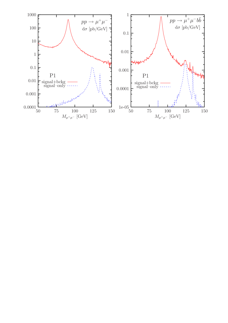
Figure 71: The differential cross section in pb/GeV as a function of the dimuon mass for the point P1, for both the signal and signal plus background in the processes $pp(\to\Phi)\to\mu^{+}\mu^{-}$ (left figure) and $pp(\to\Phi b\bar{b})\to\mu^{+}\mu^{-}b\bar{b}$ (right figure).

The differential cross sections are shown for the scenario $M_{A}=125$ GeV and $\tan\beta=30$, which leads to $M_{h}=123.3$ GeV and $M_{H}=134.3$ GeV, as a function of the invariant dimuon mass in Fig. 71 (left), for $pp(\to h,H,A)\to\mu^{+}\mu^{-}$. As can be seen, the signal rate is fairly large but when put on top of the huge Drell–Yan background, the signal becomes completely invisible. We thus conclude, that already at the level of a “theoretical simulation”, the Higgs signal will probably be hopeless to extract in this process for $M_{H}\raisebox{-3.69899pt}{~{}\shortstack{$<$ \\ [-0.07cm] $\sim$}}~{}140$ GeV. In the right-hand side of Fig. 71, we display, again for the same scenario, the signal from $pp\to\mu^{+}\mu^{-}b\bar{b}$ and the complete 4-fermion SM background as a function of the dimuon system. The number of signal events is an order of magnitude smaller than in the previous case, but one can still see the two peaks, corresponding to $h/A$ and $H$ production, on top of the background.

In order to perform a more realistic analysis, we have generated unweighted events for the full 4-fermion background $pp\to\mu^{+}\mu^{-}+b\bar{b}$ and for the signal. With the help of the new CompHEP-PYTHIA interface [407], the unweighted events have been processed through PYTHIA 6.2 [227] for fragmentation and hadronization. To simulate detector effects, such as acceptance, muon momentum smearing, and $b$–jet tagging, we take the example of the CMS detector. The details have been given in Ref. [405] and the main points are that: 1) the mass resolution on the dimuons is about 1%, and 2) the efficiency for $b$–jet tagging is of the order of 40%. The results of the simulation for a luminosity of 100 fb^-1 are shown in Fig. 72, where the number of $\mu^{+}\mu^{-}b\bar{b}$ events in bins of 0.25 GeV is shown as a function of the mass of the dimuon system. The left-hand side shows the signals with and without the resolution smearing as obtained in the Monte-Carlo analysis, while the figures in the right-hand side show also the backgrounds, including the detector effects.

For the point under consideration, the signal cross section for the heavier CP-even $H$ boson is significantly smaller than the signals from the lighter CP-even $h$ and pseudoscalar $A$ bosons; the latter particles are too too close in mass to be resolved, and only one single broad peak for $h/A$ is clearly visible. To resolve also the peak for the $H$ boson, the integrated luminosity should be increased by a factor of 3 to 4. We have also performed the analysis for $M_{A}=130$ and 135 GeV. In the former case, it would be possible to see also the second peak, corresponding to the $H$ boson signal with a luminosity of 100 fb^-1, but again the $h$ and $A$ peaks cannot be resolved. In the latter case, all three $h,A$ and $H$ bosons have comparable signal rates, and the mass differences are large enough for us to hope to be able to isolate the three different peaks, although with some difficulty.

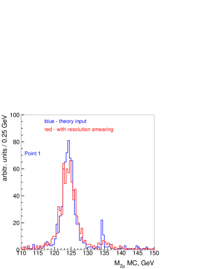
Figure 72: $\mu^{+}\mu^{-}$ pair invariant mass distributions for the signal before and after detector resolution smearing (left) and for the signal and the background (right) for $M_{A}=125$ GeV.

3 Summary

We have shown that in the intense-coupling regime, i.e. when the $h,H$ and $A$ MSSM bosons have masses too close to the critical point $M_{h}^{\rm max}$ and when the value of $\tan\beta$ is large, the detection of the individual Higgs boson peaks is very challenging at the LHC. It is only in the associated Higgs production mechanism with $b\bar{b}$ pairs, with at least one tagged $b$-jet, and with Higgs particles decaying into the clean muon-pair final states, that there is a chance of observing the three signals and resolve between them. This would be possible only if the Higgs mass differences are larger than about 5 GeV. In this note, we mostly concentrated on the fully exclusive $b\bar{b}+\mu^{+}\mu^{-}$ signature. In a more complete study, one should consider the case where only one single $b$-jet is tagged [408], and take into account also the large reducible backgrounds from $pp\to Z^{*}/\gamma^{*}\to\mu^{+}\mu^{-}$ with mistagged jets. Furthermore, once the signal peaks have been isolated, the $pp\to\mu^{+}\mu^{-}$ process can possibly be used to improve further the discrimination. Such a study is under way [409].

I. Charged Higgs Studies
K.A. Assamagan, J. Guasch, M. Guchait, J. Heyninck, S. Lowette, S. Moretti, S. Peñaranda and P. Vanlaer

1 Determining the ratio of the $H^{+}\rightarrow\tau\nu$ to $H^{+}\rightarrow t\bar{b}$ decay rates for large $\tan\beta$ at the LHC

In this note we investigate the production of charged Higgs bosons in association with top quarks at the LHC, from the experimental and theoretical point of view, by studying hadronic ($H^{+}\to t\bar{b}$) and leptonic ($H^{+}\to\tau^{+}\nu$) decay signatures. The interest of this investigation is many-fold.

• The discovery of a charged Higgs boson will point immediately to the existence of some extension of the Standard Model (SM).

• The associated production of a charged Higgs boson with a top quark ($pp\to H^{+}\bar{t}+X$) [410, 411] is only relevant at large values of $\tan\!\beta$, a regime where Higgs boson observables receive large Supersymmetric (SUSY) radiative corrections.

• While SUSY radiative effects might be difficult to discern in the production cross-sections separately, they will appear neatly in the following relation between the two mentioned channels:

  $$R\equiv\frac{\sigma(pp\to H^{+}\bar{t}+X\to\tau^{+}\nu t+X)}{\sigma(pp\to H^{+}\bar{t}+X\to t\bar{b}\bar{t}+X)}\,\,.$$ (64)

• In fact, in the ratio of (64), the dependence on the production mode (and on its large sources of uncertainty deriving from parton luminosity, unknown QCD radiative corrections, scale choices, etc.) cancels out:

  $$R=\frac{BR(H^{+}\to\tau^{+}\nu)}{BR(H^{+}\to t\bar{b})}=\frac{\Gamma(H^{+}\to\tau^{+}\nu)}{\Gamma(H^{+}\to t\bar{b})}\,\,.$$ (65)

From these remarks it is clear that the quantity $R$ is extremely interesting both experimentally and theoretically in investigating the nature of Electro-Weak Symmetry Breaking (EWSB).

In the MSSM, Higgs boson couplings to down-type fermions receive large quantum corrections, enhanced by $\tan\!\beta$. These corrections have been resummed to all orders in perturbation theory with the help of the effective Lagrangian formalism for the $t\bar{b}H^{+}$ vertex [412, 413]. The $b$-quark Yukawa coupling, $h_{b}$ , is related to the corresponding running mass at tree level by $h_{b}=m_{b}/v_{1}$. Once radiative corrections are taken into account, due to the breaking of SUSY, this relation is modified to $m_{b}\equiv h_{b}v_{1}\left(1+\Delta m_{b}\right)$ [412, 413], where $v_{i}$ is the Vacuum Expectation Value (VEV) of the Higgs doublet $H_{i}$ and $\Delta m_{b}$ is a non-decoupling quantity that encodes the leading higher order effects. Similarly to the $b$-quark case, the relation between $m_{\tau}$ and the $\tau$-lepton Yukawa coupling, $h_{\tau}$, is also modified by quantum corrections, $\Delta m_{\tau}$. We adopt in our analysis the effective Lagrangian approach by relating the fermion mass to the Yukawa coupling via a generic $\Delta m_{f}$ ($f=b,\tau$),

$$h_{f}=\frac{m_{f}(Q)}{v_{1}}\frac{1}{1+\Delta m_{f}}=\frac{m_{f}(Q)}{v\cos\beta}\frac{1}{1+\Delta m_{f}}\quad(v=(v_{1}^{2}+v_{2}^{2})^{1/2},\quad\tan\beta=\frac{v_{1}}{v_{2}})\,,$$ (66)

in which the resummation of all possible $\tan\!\beta$ enhanced corrections of the type $(\alpha_{s}\tan\!\beta)^{n}$ is included [412, 413]. The leading part of the (potentially) non-decoupling contributions proportional to soft-SUSY-breaking trilinear scalar couplings ($A_{f}$) can be absorbed in the definition of the effective Yukawa coupling at low energies and only subleading effects survive [413]. Therefore, the expression (66) contains all (potentially) large leading radiative effects. The SUSY-QCD contributions to $\Delta m_{b}$ are proportional to the Higgsino mass parameter $\Delta m_{b}\sim\mu$, while the leading SUSY-EW contributions behave like $\Delta m_{b}\sim\mu A_{t}$ [414]. Thus, they can either enhance or screen each other, depending on the sign of $A_{t}$. It is precisely these effects that will allow us to distinguish between different Higgs mechanisms of EWSB. For example, the analysis of these corrections in the ratio of neutral Higgs boson decay rates, $R^{\prime}={BR(H\to b\bar{b})}/{BR(H\to\tau^{+}\tau^{-})}$, revealed large deviations from the SM values for several MSSM parameter combinations [414]. Extensive theoretical analyses of one-loop corrections to both neutral and charged Higgs boson decays have been performed in [415, 416, 417, 418, 419, 414, 420]. We now explore the one-loop MSSM contributions to the ratio of the branching ratios ($BR\,$s) of a charged Higgs boson $H^{\pm}$ in (65), which at leading order (and neglecting kinematical factors) is given by $R=h_{\tau}^{2}/3h_{b}^{2}$ in the large $\tan\!\beta$ limit. The SUSY corrections to the $H^{+}t\bar{b}$ vertex entering the decay processes $t\to H^{+}b$ and $H^{+}\to t\bar{b}$ have been analysed in [415, 416], where it was shown that they change significantly the Tevatron limits on $m_{H^{\pm}}$ [416]. They were further explored in the production process $pp(p\bar{p})\to H^{-}t\bar{b}$ at LHC and Tevatron in [417, 418, 419, 297], where they were shown to shift significantly the prospects for discovery of a charged Higgs boson at both colliders.

Here, we have performed a detailed phenomenological analysis for the LHC of charged Higgs boson signatures, by using the subprocess $g\bar{b}\to H^{+}\bar{t}$. The QCD corrections to this channel are known to next-to-leading (NLO) [145]. However, we have normalised our production cross-section to the LO result, for consistency with the tree-level treatment of the backgrounds. In our simulation, we have let the top quarks decay through the SM-like channel $t\to W^{+}b$. In the hadronic decay channel of the charged Higgs boson ($H^{+}\to t\bar{b}$) we require one of the two $W$’s emerging from the decay chain $H^{+}\bar{t}\to(t\bar{b})\bar{t}\to(W^{+}b)\bar{b}(\bar{b}W^{-})$ to decay leptonically, to provide an efficient trigger, while the other $W$ is forced to decay hadronically, since this mode provides the largest rate and in order to avoid excessive missing energy. The $\tau$-lepton in the $H^{+}\to\tau^{+}\nu$ decay mode is searched for through hadronic one- and multi-prong channels. In summary, the experimental signatures of the two production channels under investigation are ($l=e,\mu$):

$$pp(g\bar{b}) \to H^{+}\bar{t}\to(\tau^{+}\nu)\bar{t}\to\tau^{+}\nu\,(jj\bar{b})\,\,,$$ (67)

$$pp(g\bar{b}) \to H^{+}\bar{t}\to(t\bar{b})\bar{t}\to(jj[l\nu]b)\,\bar{b}\,(l\nu[jj]\bar{b})\,\,.$$ (68)

(In the numerical analysis we always combine the signals in (67) and (68) with their charged-conjugated modes.)

The Monte Carlo (MC) simulation has been performed using PYTHIA (v6.217) [203] for the signal and most of the background processes. (We have cross-checked the signal cross-section with [145].) We have used HDECAY[165] for the Higgs boson decay rates. One of the background processes (the single-top one: see below) has been generated with TopRex [421] with a custom interface to PYTHIA. We have used ATLFAST [422] for the detector simulation. (Further details of the detector can be found in [423, 424].) We have adopted the CTEQ5L [425] parton distribution functions in their default PYTHIA v6.217 setup and we have used running quark masses derived from the pole values $m_{t}^{\rm pole}=175\,{\rm GeV}$ and $m_{b}^{\rm pole}=4.62\,{\rm GeV}$. The TAUOLA [426, 427, 428] package was interfaced to the PYTHIA event generator for treatment of the $\tau$-lepton polarisation.

The leptonic decay channel of the charged Higgs boson provides the best probe for the detection of such a state at the LHC. In fact, it turns out that despite the small branching ratio $BR(H^{+}\to\tau^{+}\nu)$, the $\tau$-lepton affords an efficient trigger to observe this channel. The production rates $\sigma\times BR(H^{+}\to\tau^{+}\nu)\times BR(W\to jj)$ are shown in Tab. 24. The main background processes in this channel are: top-pair production with one of the $W$’s decaying into $\tau\nu$ ($gg\to t\bar{t}\to jj\,b\,\tau\nu\bar{b}$) and $W^{\pm}t$ associated production ($g\bar{b}\to W^{+}\bar{t}\to\tau^{+}\nu\bar{t}$).

We have used the following trigger conditions: hadronic $\tau$-jet ($p_{T}^{\tau}>30\,{\rm GeV}$); a $b$-tagged jet ($p_{T}^{b}>30\,{\rm GeV}$) and at least two light jets ($p_{T}^{j}>30\,{\rm GeV}$). We apply afterwards a $b$-jet veto to reject the $t\bar{t}$ QCD background. As there is no isolated lepton (electron or muon) in the final state, the observation of this channel requires a multi-jet trigger with a $\tau$-trigger. After reconstructing the jet-jet invariant mass $m_{jj}$ and retaining the candidates consistent with the $W$-boson mass, $|m_{W}-m_{jj}|<25\,{\rm GeV}$, the jet four-momenta are rescaled and the associated top quark is reconstructed by minimising $\chi^{2}\equiv(m_{jjb}-m_{t})^{2}$. Subsequently, a sufficiently high threshold on the $p_{T}$ of the $\tau$-jet is required, $p_{T}^{\tau}>100\,{\rm GeV}$. The background events satisfying this cut need a large boost from the $W$-boson. This results in a small azimuthal opening angle $\Delta\phi$ between the $\tau$-jet and the missing transverse momentum, ${p\!\!\!/}_{T}$. For background suppression we then have the cut $\Delta\phi({p\!\!\!/}_{T},p_{T}^{\tau})>1$. Besides, the missing transverse momentum is harder for the signal than for the background while the differences between their distributions in azimuthal angle and missing transverse momentum increase with increasing $m_{H^{\pm}}$. These effects are well cumulated in the transverse mass, $m_{T}=\sqrt{2p_{T}^{\tau}{p\!\!\!/}_{T}\left[1-\cos(\Delta\phi)\right]}$, which provides good discrimination between the signal and the backgrounds, as shown in Fig. 73. (Further details of this kind of studies are available in [423, 424].) The discussed set of cuts reduces the total background by six orders of magnitude while the signal is only suppressed by two orders. The production rates and total detection efficiency (including detector acceptance, $b$- and $\tau$-identification, pileup and the effect of cuts) are also shown in Tab. 24 for an integrated luminosity of $300\rm\,fb^{-1}$. We can see that the signal rates are large enough to indeed consider $H^{+}\rightarrow\tau\nu$ a golden channel for the $H^{+}$ discovery at large $\tan\beta$.

Figure 73: Transverse mass $m_{T}$ distribution for signal and total background taking into account the polarisation of the $\tau$-lepton, for an integrated luminosity of $30\rm\,fb^{-1}$. A final cut $m_{T}>200$ GeV was used for the calculations of the signal-to-background ratios and for the signal significances.

	$m_{H^{\pm}}=350$	$m_{H^{\pm}}=500$	$t\bar{t}$	$W^{\pm}t$
$\sigma\times BR$	$99.9\rm\,fb$	$30.7\rm\,fb$	$79.1\rm\,pb$	$16.3\rm\,pb$
Events	29958	9219	$2.3\times 10^{6}$	$4.89\times 10^{5}$
Events after cuts	174	96	17	3
Efficiency	0.6%	1%	$8\times 10^{-6}$	$6\times 10^{-6}$
$S/B$	7.9	4.4
$S/\sqrt{B}$	37.1	20.5
Poisson	23.1	14.6

Table 24: The signal and background cross-sections, the number of events before cuts, the number of events after all cuts, the total efficiency, the signal-to-background ratios ($S/B$), and the signal significances (Gaussian and Poisson) for the detection of the charged Higgs in the $\tau\nu$ channel at the LHC, for $300\rm\,fb^{-1}$ integrated luminosity and $\tan\!\beta=50$.

The production rates $\sigma\times BR(H^{+}\to t\bar{b})\times BR(W^{+}W^{-}\to jjl\nu)$ are shown in Tab. 25. The decay mode $H^{\pm}\to tb$ has large QCD backgrounds at hadron colliders that come from $t\bar{t}q$ production with $t\bar{t}\rightarrow Wb\,Wb\rightarrow l\nu b\,jjb$. However, the possibility of efficient $b$-tagging has considerably improved the situation [429, 430, 293]. We search for an isolated lepton ($p_{T}^{e}>20\,{\rm GeV}$, $p_{T}^{\mu}>8\,{\rm GeV}$), three $b$-tagged jets ($p_{T}^{b}>30\,{\rm GeV}$) and at least two non $b$-jets ($p_{T}^{j}>30\,{\rm GeV}$). We retain the jet-jet combinations whose invariant masses are consistent with the $W$-boson mass, $|m_{W}-m_{jj}|<25\,{\rm GeV}$, then we use the $W$-boson mass constraint to find the longitudinal component of the neutrino momentum in $W^{\pm}\to l\nu$, by assuming that the missing transverse momentum belongs only to the neutrino. Subsequently, the two top quarks entering the $H^{+}\bar{t}\to(t\bar{b})\bar{t}\to(jj[l\nu]b)\,\bar{b}\,(l\nu[jj]\bar{b})$ decay chain are reconstructed, retaining the pairing whose invariant masses $m_{l\nu b}$ and $m_{jjb}$ minimise $\chi^{2}\equiv(m_{t}-m_{l\nu b})^{2}+(m_{t}-m_{jjb})^{2}$. The remaining $b$-jet can be paired with either top quark to give two charged Higgs candidates, one of which leads to a combinatorial background. The expected rates for signal and background (after the mentioned decays) are shown in Tab. 25. (This analysis is presented extensively in [423, 424].)

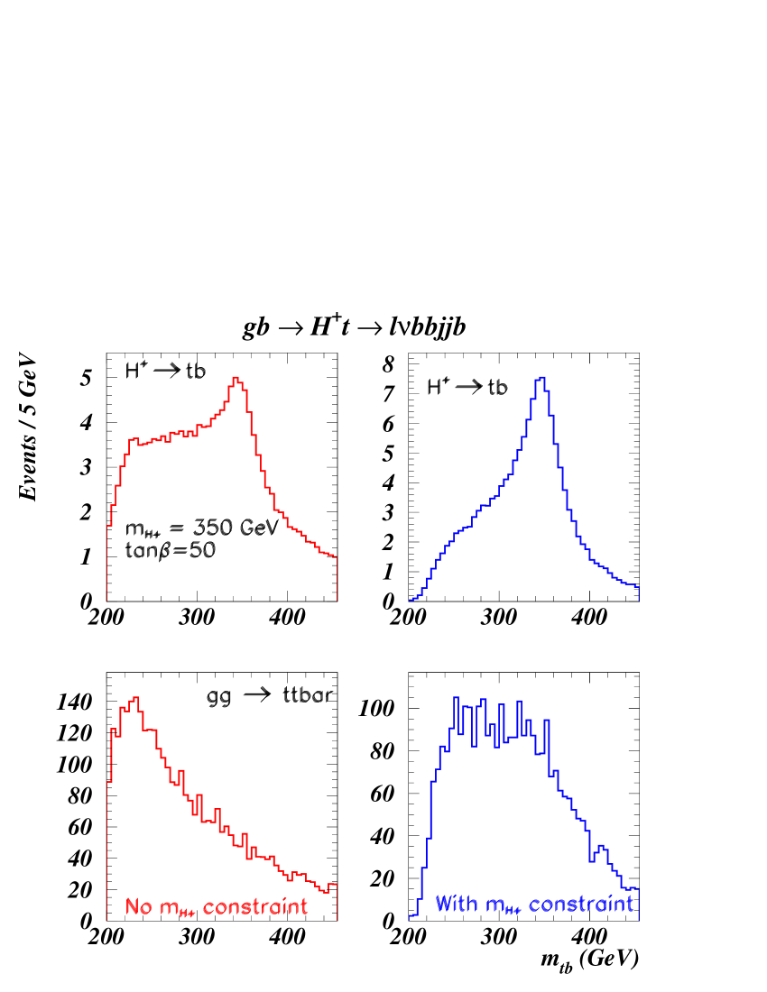
Figure 74: The signal and the background distributions for the reconstructed invariant mass $m_{tb}$ of $m_{H^{\pm}}=350\,{\rm GeV}$, $\tan\beta=50$ and an integrated luminosity of $30\rm\,fb^{-1}$. Assuming that the charged Higgs is discovered in the $H^{\pm}\to\tau\nu$ channel, one can use $m_{H^{\pm}}$ as a constraint to reduce the combinatorial background: this is shown on the right plots.

At this point, we have two charged Higgs candidates: $t_{1}b_{3}$ or $t_{2}b_{3}$. Assuming that the charged Higgs is discovered through the $H^{\pm}\to\tau\nu$ channel and its mass determined from the $\tau\nu$ transverse mass distribution [423, 424], the correct charged Higgs candidate in the $tb$ channel can be selected by using the measured $m_{H^{\pm}}$ as a constraint. This is done by selecting the candidate whose invariant mass is closest to the measured charged Higgs mass: $\chi^{2}=(m_{tb}-m_{H^{\pm}})^{2}$. The signal distribution for the reconstructed invariant mass $m_{tb}$ for a charged Higgs boson weighing $350\,{\rm GeV}$, with $\tan\beta=50$ and after integrated luminosity of $30\rm\,fb^{-1}$, is shown in Fig. 74. We can see that for the $H^{+}\rightarrow t\bar{b}$ decay some irreducible combinatorial noise still appears even when the $m_{H^{\pm}}$ constraint is included. In addition, for the background, we have found that the $m_{H^{\pm}}$ constraint reshapes the distributions in $gg\rightarrow t\bar{t}X$ in such a way that no improvement in the signal-to-background ratio and signal significance is further observed. Finally, recall that the knowledge of the shape and the normalisation of the reshaped background would be necessary for the signal extraction. For these reasons, we did not use the $m_{H^{\pm}}$ constraint for the results shown in this work. The subtraction of the background can then be done by fitting the side bands and extrapolating in the signal region which will be known from the $m_{H^{\pm}}$ determination in the $H^{\pm}\to\tau\nu$ channel: however, this would be possible only for Higgs masses above $300\,{\rm GeV}$ – see Fig. 74. The signal and background results are summarised in Tab. 25 at an integrated luminosity of $300\rm\,fb^{-1}$ for different values of $m_{H^{\pm}}$ and $\tan\beta=50$. It is shown that it is difficult to observe $H^{\pm}$ signals in this channel above $\sim 400\,{\rm GeV}$, even with the $m_{H^{\pm}}$ constraint. For masses above $m_{H^{\pm}}\sim 400\,{\rm GeV}$ the signal significance can be enhanced by using the kinematics of the three-body production process $gg\to H^{+}\bar{t}b$ [417, 418, 419, 429, 430, 293].

We assume a theoretical uncertainty of $5\%$ on the branching ratios, $BR\,$s. Previous ATLAS studies have shown the residual $gg\to t\bar{t}$ shape and normalisation can be determined to $5\%$ [423, 424]. The scale uncertainties on jet and lepton energies are expected to be of the order $1\%$ and $0.1\%$ respectively [423, 424]. As explained above, for $m_{H^{\pm}}>300$ GeV, the side band procedure can be used the subtract the residual background under the $H^{+}\rightarrow tb$ signal: we assume also a $5\%$ uncertainty in the background subtraction method. Thus, the statistical uncertainties can be estimated as $\sqrt{1/S}$. The uncertainty in the ratio $R$ are dominated by the reduced knowledge of the background shape and rate in the $H^{+}\rightarrow tb$ channel. The cumulative results for the two channels are summarised in Tab. 26 at an integrated luminosity of $300\rm\,fb^{-1}$. Here, the final result for the ratio $R$ is obtained by correcting the visible production rates after cuts for the total detection efficiency in Tabs. 24 and 25 and by the decay $BR\,$s of the $W$-bosons. The simulation shows that the above mentioned ratio can be measured with an accuracy of $\sim 12-14\%$ for $\tan\beta=50$, for $m_{H^{\pm}}=300-500\,{\rm GeV}$ and at an integrated luminosity of $300\rm\,fb^{-1}$.

We turn now to the impact of the SUSY radiative corrections. Their role is twofold. Firstly, by changing the value of the Yukawa coupling they change the value of the observable $R$. Secondly, they can change the value of the production cross-section $\sigma(pp\to H^{+}\bar{t}+X)$, hence shifting significantly (by as much as $100\,{\rm GeV}$) the range of charged Higgs masses accessible at the LHC [417, 418, 419].

	$m_{H^{\pm}}=350$	$m_{H^{\pm}}=500$	$t\bar{t}q$
$\sigma\times BR$	$248.4\rm\,fb$	$88\rm\,fb$	$85\rm\,pb$
Events	74510	26389	$2.55\times 10^{7}$
Events after cuts	2100	784	59688
Efficiency	2.8%	3%	0.2%
$S/B$	0.035	0.013
$S/\sqrt{B}$	8.6	3.2

Table 25: The signal and background cross-sections, the number of events before cuts, the number of events after all cuts, total efficiency, $S/B$, and the signal significances for the detection of the charged Higgs in the $tb$ channel at the LHC, for $300\rm\,fb^{-1}$ integrated luminosity and $\tan\!\beta=50$.

	$m_{H^{\pm}}=350$	$m_{H^{\pm}}=500$
Signals $\tau\nu/tb$	174 / 2100 = 0.08	96 / 784 = 0.12
Signals (corrected) $\tau\nu/tb$	0.18	0.16
Systematics unc.	$\sim 9\%$	$\sim 9\%$
Total unc.	12%	14%
Theory	0.18	0.16

Table 26: Experimental determination of the ratio (64) for $300\rm\,fb^{-1}$ and $\tan\!\beta=50$. Shown are: the signal after cuts, the signal after correcting for efficiencies and branching ratios, the systematic uncertainty, the total combined uncertainty, and the theoretical prediction (without SUSY corrections).

To explore the second consequence, we rely on the fact that the bulk of the SUSY corrections to the production cross-section is given by the Yukawa coupling redefinition in (66) [417, 418, 419, 145]. By neglecting the kinematic effects, taking the large $\tan\!\beta$ limit and assuming that the dominant decay channel of the charged Higgs boson is $H^{+}\to t\bar{b}$ (large mass limit), we can estimate the corrected production rates. For simplicity, we show only the contributions to $\Delta m_{b}$, since they are the dominant ones:

$$\sigma^{\rm{corr}}(g\bar{b}\to H^{+}\bar{t}\to t\bar{b}\bar{t}) = \sigma^{\rm{corr}}(g\bar{b}\to H^{+}\bar{t})\times BR^{\rm{corr}}(H^{+}\to t\bar{b})\simeq\frac{\sigma^{0}(g\bar{b}\to H^{+}\bar{t})}{(1+\Delta m_{b})^{2}}\,\,,$$

$$\sigma^{\rm{corr}}(g\bar{b}\to H^{+}\bar{t}\to\tau^{+}\nu\bar{t}) = \sigma^{\rm{corr}}(g\bar{b}\to H^{+}\bar{t})\times\frac{\Gamma(H^{+}\to\tau^{+}\nu)}{\Gamma^{\rm{corr}}(H^{+}\to t\bar{b})}$$ (69)

$$\simeq \frac{\sigma^{0}(g\bar{b}\to H^{+}\bar{t})}{(1+\Delta m_{b})^{2}}\times\frac{\Gamma(H^{+}\to\tau^{+}\nu)}{\Gamma^{0}(H^{+}\to t\bar{b})\times\frac{1}{(1+\Delta m_{b})^{2}}}\,\,.$$

This very simple exercise shows that the production rate in the $\tau$-channel is fairly independent of the SUSY radiative corrections and therefore the tree-level analysis performed above can (to a very good approximation) be used for our original purposes. Actually, once we take into account kinematical effects, the $\tau$-channel will receive small (negative) corrections in the low charged Higgs mass range. However, in this range, $BR(H^{+}\to\tau^{+}\nu)$ is quite large and one should not fear to loose the signal. Quite the opposite, the hadronic $t\bar{b}$ production channel receives large radiative corrections. These corrections can be either positive (enhancing the signal, and therefore the significance in Tab. 25) or negative (reducing it, possibly below observable levels). In Fig. 75a, we show the discussed enhancement/suppression factors as a function of $\tan\!\beta$ for $m_{H^{\pm}}=350\,{\rm GeV}$ and a SUSY mass spectrum defined as SPS4 of the Snowmass Points and Slopes in [431], but choosing different scenarios for the sign of $\mu$ and $A_{t}$. (It is worth noting that the production rate for the $tb$-channel can be enhanced by a factor larger than 3 in some SUSY scenarios, which would enhance significantly the corresponding signal thus overcoming the low signal-to-background ratio of this channel.)

(a)	(b)

Figure 75: a) Production rates enhancement/suppression factors for the $\tau$ and the $tb$ channels; b) the SUSY correction to the rate (65). Plots as functions of $\tan\!\beta$ for $m_{H^{\pm}}=350\,{\rm GeV}$ and a SUSY spectrum as in SPS4, but for different choices of the signs of $\mu$ and $A_{t}$. Shown is also the experimental determination for each scenario.

We now turn our attention to the observable under analysis. Fig. 75b shows the prediction for the ratio $R$ as a function of $\tan\!\beta$ for the SPS4 scenario with a charged Higgs mass of $m_{H^{\pm}}=350\,{\rm GeV}$. The value of $R$ only depends on $m_{H^{\pm}}$ through kinematical factors and the dependence is weak for $m_{H^{\pm}}\stackrel{{\scriptstyle\scriptstyle>}}{{{}_{\sim}}}300\,{\rm GeV}$. In this figure, we also show the experimental determination carried out as before and repeated for each SUSY setup. From Fig. 75b it is clear that radiative SUSY effects are visible at the LHC at a large significance. In particular, the $\mu<0$ scenarios can easily be discriminated, while the $\mu>0$ ones will be more difficult to establish, due to the lower signal rate of the hadronic channel. This feature then also allows for a measurement of the sign of the $\mu$ parameter. In contrast, since radiative corrections are independent of the overall SUSY scale, the observable $R$ cannot provide us with an estimation of the typical mass of SUSY particles. Nonetheless, the information obtained in other production channels (e.g., neutral Higgs bosons or SUSY particles direct production) can be used to perform precision tests of the MSSM.

To summarise, we have used the observable $R\equiv\frac{\sigma(pp\to H^{+}\bar{t}+X\to\tau^{+}\nu t+X)}{\sigma(pp\to H^{+}\bar{t}+X\to t\bar{b}t+X)}=\frac{BR(H^{+}\to\tau^{+}\nu^{-})}{BR(H^{+}\to t\bar{b})}\,$ to discriminate between SUSY and non-SUSY Higgs models. This quantity is a theoretically clean observable. The experimental uncertainties that appear in this ratio have been analysed in details through detailed phenomenological simulations. In the MSSM, $R$ is affected by quantum contributions that do not decouple even in the heavy SUSY mass limit. We have quantitatively shown that an LHC measurement of $R$ can give clear evidence for or against the SUSY nature of charged Higgs bosons.

2 Charged Higgs Bosons in the Transition Region ${M_{H^{\pm}}\sim m_{t}}$ at the LHC

2.1 The Threshold Region

The detection of charged Higgs bosons ($H^{\pm}$) would unequivocally imply the existence of physics beyond the Standard Model (SM), since spin-less charged scalar states do not belong to its particle spectrum. Singly charged Higgs bosons appear in any Two-Higgs Doublet Model (2HDM), including a Type-II in presence of minimal Supersymmetry (SUSY), namely, the Minimal Supersymmetric Standard Model (MSSM). Depending on its mass, the machines that are likely to first discover such a state are Tevatron $p\bar{p}$ ($\sqrt{s}=2$ TeV) and the LHC ($\sqrt{s}=14$ TeV). Current limits on the charged Higgs boson mass are set by LEP at about 80 GeV. At the Tevatron a charged Higgs boson could be discovered for masses up to $m_{t}-m_{b}$, whereas the LHC has a reach up to the TeV scale, if $\tan\beta$ is favourable (i.e., either large or small).

For the LHC, the ATLAS discovery potential of $H^{\pm}$ bosons in a general Type-II 2HDM or MSSM (prior to the results of this study) is visualised in the left-hand side of Fig. 76. (A similar CMS plot, also including neutral Higgs states, is given for comparison.) The existence of a gap in coverage for $M_{H^{\pm}}\approx m_{t}$ was already denounced in Refs. [62, 392] as being due to the fact that Monte Carlo (MC) simulations of $H^{\pm}$ production for $M_{H^{\pm}}\sim m_{t}$ were flawed by a wrong choice of the hard scattering process. In fact, for $M_{H^{\pm}}<m_{t}$, the estimates in both plots in Fig. 76 were made by assuming as main production mode of $H^{\pm}$ scalars the decay of top (anti)quarks produced via QCD in the annihilation of gluon-gluon and quark-antiquark pairs (hence – by definition – the attainable Higgs mass is strictly confined to the region $M_{H^{\pm}}\leq m_{t}-m_{b}$). This should not be surprising (the problem was also encountered by CMS, see right-hand side of Fig. 76), since standard MC programs, such as PYTHIA and HERWIG [432, 294], have historically accounted for this process through the usual procedure of factorising the production mode, $gg,q\bar{q}\to t\bar{t}$, times the decay one, $\bar{t}\to\bar{b}H^{-}$, in the so-called Narrow Width Approximation (NWA) [297]. This description fails to correctly account for the production phenomenology of charged Higgs bosons when their mass approaches or indeed exceeds that of the top-quark (i.e., falls in the so called ‘threshold region’). This is evident from the left plot in Fig. 77. (The problem also occurs at Tevatron, see right plot therein and Refs. [297, 433].) As remarked in Ref. [297], the use of the $2\to 3$ hard scattering process $gg,q\bar{q}\to t\bar{b}H^{-}$ [410]–[418], in place of the ‘factorisation’ procedure in NWA, is mandatory in the threshold region, as the former correctly keeps into account both effects of the finite width of the top quark and the presence of other $H^{\pm}$ production mechanisms, such as Higgs-strahlung and $b\bar{t}\to H^{-}$ fusion (and relative interferences). The differences seen between the two descriptions in Fig. 77 are independent of $\tan\beta$ and also survive in, e.g., $p_{T}$ and $\eta$ spectra [297].

One more remark is in order, concerning the LHC plot in Fig. 77. In fact, at the CERN hadron collider, the above $2\to 3$ reaction is dominated by the $gg$-initiated subprocesses, rather than by $q\bar{q}$-annihilation, as is the case at the Tevatron. This means that a potential problem of double counting arises in the simulation of $tH^{-}X$ + c.c. events at the LHC, if one considers that Higgs-strahlung can also be emulated through the $2\to 2$ process $bg\to tH^{-}$ + c.c., as was done in assessing the ATLAS (and CMS) discovery reaches in the $H^{+}\to t\bar{b}$ and $H^{+}\to\tau^{+}\nu_{\tau}$ channels for $M_{H^{\pm}}>m_{t}$ (see Refs. [423, 398] for reviews). The difference between the two approaches is well understood, and prescriptions exist for combining the two, either through the subtraction of a common logarithmic term [292, 430] or by means of a cut in phase space [418].

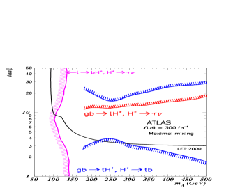
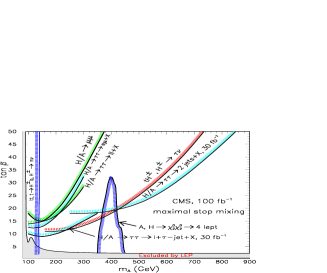
Figure 76: The ATLAS 5-$\sigma$ discovery contours of 2HDM charged Higgs bosons for 300 fb^-1 of luminosity, only including the reach of SM decay modes (left plot). The CMS 5-$\sigma$ discovery contours of MSSM Higgs bosons for 100 fb^-1 of luminosity, also including the reach of $H,A\to\chi^{0}_{2}\chi^{0}_{2}\to 4l^{\pm}$ decays, assuming $M_{1}$ = 90 GeV, $M_{2}$ = 180 GeV, $\mu$ = 500 GeV, $M_{\tilde{\ell}}$ = 250 GeV, $M_{\tilde{q},\tilde{g}}$ = 1000 GeV (right plot).

If one then looks at the most promising (and cleanest) charged Higgs boson decay channel, i.e., $H^{\pm}\to\tau^{\pm}\nu_{\tau}$ [437], while using the $gg,q\bar{q}\to t\bar{b}H^{-}$ + c.c. description and reconstructing the accompanying top quark hadronically, the prospects of $H^{\pm}$ detection should improve significantly for $M_{H^{\pm}}$ values close to $m_{t}$, eventually leading to the closure of the mentioned gap. The $2\to 3$ description of the $H^{\pm}$ production dynamics (as well as the spin correlations in $\tau$-decays usually exploited in the ATLAS $H^{\pm}\to\tau^{\pm}\nu_{\tau}$ analysis) have been made available in version 6.4 [395] of the HERWIG  event generator (the latter also through an interface to TAUOLA [426]), so that detailed simulations of $H^{\pm}$ signatures at both the Tevatron and the LHC are now possible for the threshold region, including fragmentation/hadronisation and detector effects. In the next section we will discuss the details of an ATLAS analysis based on such tools that has lead to the closure of the mentioned gap through the discussed charged Higgs decay channel. This analysis was initiated in the context of the 2003 Les Houches workshop.

Figure 77: Cross section for $gg,q\bar{q}\to t\bar{b}H^{-}$, $gg,q\bar{q}\to t\bar{t}\to t\bar{b}H^{-}$ with finite top quark width, $bg\to tH^{-}$ and the combination of the first and the last, at the LHC with $\sqrt{s}=14$ TeV (left plot). Cross section for $gg,q\bar{q}\to t\bar{b}H^{-}$ and $gg,q\bar{q}\to t\bar{t}\to t\bar{b}H^{-}$ in NWA, at the Tevatron with $\sqrt{s}=2$ TeV (right plot). Rates are function of $M_{H^{\pm}}$ for a representative value of $\tan\beta$.

2.2 Analysis

The signal $gg\to tbH^{\pm}\to jjbb\tau\nu$ and the major backgrounds, $gg\to t\bar{t}\to jjb\tau\nu b$ and $q\bar{q},qg,\bar{q}g\to W+\mbox{jets}$, are generated with HERWIG v6.4 in the default implementation except for CTEQ5L [438] Parton Distribution Functions (PDFs). The detector is simulated with ATLFAST [359]. The TAUOLA package [426] is used for the polarisation of the $\tau$-lepton. The selection of the final state requires a multi-jet trigger with a $\tau$-trigger:

(1)  

We search for one hadronic $\tau$-jet, two $b$-tagged jets and at least two light-jets, all with $p_{T}>30$ GeV. Furthermore, the $\tau$-jet and the $b$-tagged jets are required to be within the tracking range of the ATLAS Inner Detector, $|\eta|<2.5$. We assume a $\tau$-tagging efficiency of 30% and a $b$-tagging efficiency of 60%(50%) at low(high) luminosity. The efficiency of this selection is at the level of 1.31% for the signal (e.g., at $M_{H^{\pm}}=170$ GeV), 1.25% for $gg\to t\bar{t}\to jjb\tau\nu b$ events and $(0.36\,\times\,10^{-3})$% for $W^{\pm}$+jets events.

(2)  

We reconstruct the invariant masses of pairs of light-jets, $m_{jj}$, and keep those consistent with the $W^{\pm}$ mass: $|m_{jj}-M_{W}|<25$ GeV. The associated top-quark is then reconstructed requiring $|m_{jjb}-m_{t}|<25$ GeV. For the signal with a charged Higgs mass of 170 GeV, 0.68% of signal events pass this selection criteria compared to 0.73% and $(0.45\,\times\,10^{-6})$% for the $t\bar{t}$ and $W^{\pm}$+jets backgrounds, respectively.

(3)  

We require that the transverse momentum of the $\tau$-jet be greater than 100 GeV, the transverse missing momentum be greater than 100 GeV and the azimuthal opening angle between the $\tau$-jet and the missing momentum vector be greater than one radian. Indeed, in the signal, the $\tau$-lepton originates from a scalar particle ($H^{\pm}$) whereas in the background the $\tau$-lepton comes from the decay of a vector particle ($W^{\pm}$). This difference reflects in the polarisation state of the $\tau$ and leads to harder $\tau$-jets in the signal compared to the backgrounds [423]–[429]. Furthermore, to satisfy the large cut on the transverse missing momentum and because the charged Higgs is heavier than the $W^{\pm}$-boson, a much larger boost is required from the $W^{\pm}$- in the background than from the $H^{\pm}$-boson in the signal. As a result, the spectra of the azimuthal opening angle between the $\tau$-jet and the missing transverse momentum are different for signals and backgrounds, as shown in Fig. 78 (left plot).

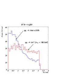
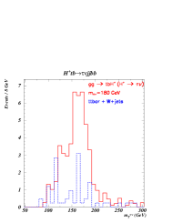
Figure 78: The plot on the left shows the azimuthal opening angle between the $\tau$-jet and the transverse missing momentum. It peaks forward in the background and more and more backward in the signal, as the charged Higgs mass increases. The right plot shows the reconstructed transverse mass for a 180 GeV Higgs. (Both plots are shown for an integrated luminosity of 30 fb^-1.)

Although the full invariant mass of the $H^{\pm}\to\tau\nu$ system cannot be reconstructed because of the neutrino in the final state, the transverse mass (which is kinematically constrained to be below the $W^{\pm}$-mass in the backgrounds and below the $H^{\pm}$-mass in the signal)

$$m_{T}=\sqrt{2p_{T}^{\tau-{\rm jet}}{p\!\!\!/}_{T}\left[1-\cos(\Delta\phi)\right]}$$ (70)

combines the benefits of both the polarisation effects and the kinematic boost, thus providing a good discriminating observable, as shown in Fig. 78 (right plot). (The residual background under the signal is due to the experimental $E_{T}^{\rm{miss}}$ resolution.)

(4)  

We also apply a combination of other cuts on: the invariant mass and the azimuthal opening angle of the $\tau b$-jet system, where $b$-jet is here the remaining one after the reconstruction of the top quark ($m_{\tau b-{\rm{jet}}}>$ 100 GeV and $\Delta\Phi(\tau-{\rm{jet}},b-{\rm{jet}})>1.25$ radians); the invariant mass of the $b\bar{b}$ pair ($m_{bb-{\rm{jet}}}>225$ GeV) and the transverse mass of the $\tau b$-jet system ($p_{T}^{\tau b-{\rm{jet}}}>190$ GeV). The cumulative effect of these cuts is the reduction of the $W^{\pm}$+jets background by more than one order of magnitude, while the signal ($M_{H^{\pm}}=$ 170 GeV) and the $t\bar{t}$ background are suppressed by only a factor of two.

(5)  

Finally, we require $m_{T}>100$ GeV for the calculation of the signal-to-background ratios and the signal significances in Tab. 27. This cut is very efficient against the $t\bar{t}$ noise (the efficiency is 0.06% for a $M_{H^{\pm}}=170$ GeV Higgs signal, $1.9\,\times\,10^{-3}$ and $0.42\,\times\,10^{-6}$ for the $t\bar{t}$ and the $W^{\pm}$+jets backgrounds, respectively).

Table 27: Sensitivity of the ATLAS detector to the observation of charged Higgs bosons through $H^{\pm}\rightarrow\tau\nu$ decays in the transition region, for an integrated luminosity of 30 fb^-1 and $\tan\beta=50$.

$M_{H^{\pm}}$ (GeV)	160	170	180	190
Signal ($S$)	35	46	50	35
Backgrounds ($B$)	13	13	13	13
$S/B$	2.7	3.5	3.8	2.7
$S/\sqrt{B}$	9.7	12.8	13.9	9.7
Poisson Significance	7.3	9.1	9.8	7.3
Poisson Significance$+$5% syst.	7.1	8.9	9.5	7.1

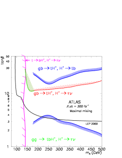
Figure 79: The new ATLAS discovery potential for charged Higgs bosons. The results of the current analysis are shown in green.

2.3 Results

The discovery contour in the transition region resulting from this new analysis is shown in Fig. 79. Notice that, at lower masses, the signal reconstruction efficiency decreases (although the rate is higher), thus explaining the upward turn of the discovery reach.

Before closing, some additional information is in order regarding the interplay between the new curve and the two old ones. In fact, recall that above the top-quark mass, the $2\to 2$ process, $bg\to tH^{-}$, with $H^{\pm}\to\tau\nu$, was used while below it the charged Higgs was searched for in top-quark decays, $t\to bH^{\pm}$, counting the excess of $\tau$-leptons over the SM expectations. Furthermore, in the analysis above the top-quark mass, CTEQ2L PDFs [438] were used and the charged Higgs production cross sections were obtained from another generator, PYTHIA v5.7. These differences complicate the matching of the various contours at their boundaries, especially between the transition region and the high mass region ($M_{H^{\pm}}>m_{t}$). In the result shown, the normalisation cross sections for the transition region were matched to the PYTHIA v5.7 numbers above $m_{t}$, for consistency with the previous analysis of the high mass region [423]. A second stage of this analysis is currently underway to update all the discovery contours by adopting the same $2\to 3$ production process throughout.

2.4 Conclusions

Meanwhile, as ad interim conclusion, we would like to claim that the LHC discovery potential of charged Higgs bosons has been extended further by our preliminary analysis.

3 Heavy Charged MSSM Higgs Bosons in the $H^{\pm}\to tb$ Decay in CMS

3.1 Introduction

One of the most straightforward ways to extend the Standard Model, is to add an extra complex Higgs doublet to the theory, thus giving rise to five physical Higgs bosons after electroweak symmetry breaking [439], two of which are the charged scalars $H^{\pm}$. A particular example of a model containing two Higgs doublets, is the much investigated Minimal Supersymmetric Standard Model (MSSM).

The production cross section and decay modes of the charged Higgs $H^{\pm}$, can be described in the MSSM by two parameters at tree level. These are usually taken as the ratio of the vacuum expectation values of the two Higgs doublets $\tan\beta=v_{2}/v_{1}$, and the mass of the pseudoscalar Higgs $m_{A}$. This mass $m_{A}$ is, again at tree level, related to the charged Higgs boson mass as $m_{A}^{2}=m_{H^{\pm}}^{2}-m_{W^{\pm}}^{2}$. The branching ratios for the decay channels of the charged Higgs, depend mainly on its mass. As shown in Fig. 81, for masses above $m_{t}+m_{b}$, the channel $H^{\pm}\to tb$ dominates. In the main production channel $gb\to tH^{\pm}$, it will result in complex final states, the most interesting being the semileptonic one,

$$gb\to tH^{\pm}\to ttb\to W^{+}W^{-}bbb\to qq^{\prime}\ell\nu bbb,$$ (71)

because the Higgs boson mass can still be reconstructed, while an isolated lepton is present to trigger on.

Figure 80: Charged Higgs boson branching ratios in function of $m_{A}$, generated with HDECAY.

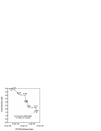
Figure 81: Evolution through time of the PYTHIA cross section value for $gb\to tH^{\pm}$. The PYTHIA version is shown in the labels on the curve. ($m_{A}=300\,\mathrm{GeV}$, $\tan\beta=50$)

The potential of the decay channel $H^{\pm}\to tb$ for high Higgs boson masses at LHC, has been considered before at parton level in several phenomenological studies [411, 410, 430, 293, 62]. These studies showed the possibility of detecting the charged Higgs in certain regions of $(m_{A},\tan\beta)$ parameter space during the low luminosity run of LHC, with both three or four $b$–jets tagged, provided good $b$–tagging capabilities of the detectors to suppress the large $t\bar{t}+\mathrm{jets}$ background. Fast simulation studies, taking into account parametrized detector performances, have also been carried out for CMS [440] and ATLAS [441, 442].

In this analysis, charged Higgs detection has been studied for the final state (71) using triple $b$–tagging, during the low luminosity period where LHC will acquire an integrated luminosity $L=\int\mathcal{L}dt=60\,\mathrm{fb}^{-1}$ of data. Supersymmetric particles are supposed heavy enough, so that decays into them can be neglected. The main improvement of this analysis, is the inclusion of the most recent theoretical calculation[145] for the signal cross section at leading order (LO) and next–to–leading order (NLO), leading to sizable effects compared to the previous discovery prospects. Indeed, the leading order cross section values, predicted by the Monte–Carlo program PYTHIA [203], have decreased by a factor $\sim 3$ over the last 5 years, as shown in Fig. 81. Other improvements are the use of a new dedicated background simulation, the inclusion of CMS trigger acceptances, the introduction of a likelihood based method to suppress the combinatorial background and the estimation of the influence of systematic uncertainties on the background cross section.

3.2 Signal and Background Simulation

The production of the charged Higgs boson is considered in the dominant inclusive channel $pp\to tH^{\pm}\!X$. The cross section for this process should be evaluated at leading order in the channel $gb\to tH^{\pm}$ [145]. Its dependency on $\tan\beta$ and $m_{A}$ has been visualized in Figs. 83 and 83. The cross section decreases exponentially with rising $m_{A}$, and is enhanced at low and high values of $\tan\beta$, with a minimum at $\tan\beta=\sqrt{m_{t}/m_{b}}$. The calculation of the signal cross section has also been performed at NLO [145]. The resulting increase in cross section depends on the value of the MSSM parameters. In the mass region considered and for $\tan\beta>30$, however, the signal $k$–factor keeps the constant value $k=1.3$.

Figure 82: $pp\to tH^{\pm}X$ cross section dependence on $m_{A}$.

Figure 83: $pp\to tH^{\pm}X$ cross section dependence on $\tan\beta$.

The generation of the signal has been performed with PYTHIA, using the cross section values from [145, 443], and forcing the $H^{\pm}\to tb$ decay. The branching ratios for this decay process were calculated with HDECAY [165], ranging from $\sim 80\%$ for low $m_{A}$ and high $\tan\beta$ up to $\sim 100\%$ for high $m_{A}$ and low $\tan\beta$, as also shown in Fig. 81. Six samples have been generated at $\tan\beta=50$ and masses $m_{A}$ ranging from $250\,\mathrm{GeV}$ to $500\,\mathrm{GeV}$. This yields a number of signal events before the event selection of almost $55\,000$ for $m_{A}=250\,\mathrm{GeV}$ down to about $7\,500$ for $m_{A}=500\,\mathrm{GeV}$.

At leading order, the dominant background comes from Standard Model $gb\to t\bar{t}b$ and $t\bar{t}+\mathrm{jet}$ production, where in the latter case the accompanying quark or gluon jet is misidentified as being a $b$–jet. Other potential multi–jet backgrounds are much smaller [411, 444] and neglected. The aforementioned background processes cannot be generated with PYTHIA. Therefore the simulation of the background has in the first place been performed by generating $t\bar{t}$ events with PYTHIA, where the parton shower generates additional jets. An overall LO cross section of $560\,\mathrm{pb}$ was used, resulting in about $17\times 10^{6}$ events before the event selection. This background will further be referred to, as the $t\bar{t}$ background.

The background simulation has also been performed using the matrix element generator MadGraph/MadEvent [445], in order to simulate directly the hard interactions $pp\to t\bar{t}b$ and $pp\to t\bar{t}j$. A cut on the transverse momentum $p_{T}>10\,\mathrm{GeV}$ and the pseudorapidity $\left|\eta\right|<2.5$ of the extra jet accompanying the tops was applied, resulting in a total cross-section of $678\,\mathrm{pb}$, or over $20\times 10^{6}$ events before selection. After the simulation of the hard interaction, the events were interfaced to PYTHIA for parton showering, decay and hadronisation. This background will further be called the $t\bar{t}b/t\bar{t}j$ background.

When looking at next–to–leading order, the cross section for the $t\bar{t}$ background scales up to about $800\,\mathrm{pb}$ [446]. This rise has been taken into account by using a $k$–factor of $k=1.43$ for the $t\bar{t}$ background when quoting results at NLO. The calculation for the processes $pp\to t\bar{t}b$ and $pp\to t\bar{t}j$ at NLO has not been performed yet, however, and therefore no NLO comparison has been made for this background.

3.3 Event Selection and Triggering

To simulate CMS detector performance, the programs CMSJET [447] and FATSIM [448] have been used for detector response parametrization. In this study, $b$–tagging is performed with a method based on impact parameter significance. For both the background samples, the $b$–tagging efficiency was found to be about 45%, while for the signal this efficiency grows from 44% to 48%, due to the harder event kinematics, with $m_{A}$ going from $250\,\mathrm{GeV}$ to $500\,\mathrm{GeV}$. This behaviour is also observed in the light quark mistag rate, ranging from 1.10% to 1.18% with rising $m_{A}$. For the background, this mistag rate is significantly different for both background samples. For the $t\bar{t}$ and $t\bar{t}b/t\bar{t}j$ background, the mistag probability was found to be 0.92% and 1.02% respectively. This is a result of the harder event kinematics in the $t\bar{t}b/t\bar{t}j$ background compared to the $t\bar{t}$ one.

In order to be able to reconstruct an event, a selection is performed, accepting only those events for which the reconstruction yields at least

• 1 isolated lepton (electron or muon) with $|\eta|<2.4$ and $p_{T}>19\,\mathrm{GeV}$ for muons and $p_{T}>29\,\mathrm{GeV}$ for electrons.

• 5 jets ($b$ or non $b$) with $p_{T}>20\,\mathrm{GeV}$ and $|\eta|<2.4$. Jets are reconstructed using a cone algorithm with $\Delta R=\sqrt{\Delta\phi^{2}+\Delta\eta^{2}}=0.5$.

• 3 $b$–tagged jets.

The total efficiency of these criteria on the different background and signal samples, is shown in the third column of Table 28 for $\tan\beta=50$ and $30\,\mathrm{fb}^{-1}$ of integrated luminosity. The low efficiency is mainly due to the demand for three $b$–tagged jets, allowing for the suppression of the background one order of magnitude more than the signal. When comparing the efficiency for the $t\bar{t}b/t\bar{t}j$ background with the $t\bar{t}$ background, the difference is found to be mainly due to the higher mistag rate.

In order to estimate the influence of the CMS trigger acceptances on the event rate of reconstructable events, the High Level Trigger (HLT) cuts are applied only after these minimal selection criteria. As an isolated lepton is present in the final state, high triggering efficiencies are expected with only the inclusive electron and muon triggers. The HLT cuts at low luminosity are taken at $29\,\mathrm{GeV}$ for single electrons and $19\,\mathrm{GeV}$ for single muons [449]. Additionally, a correction factor of 68.9% was applied on the events with an electron, to account for inefficiencies in the online electron reconstruction [449].

For as well the backgrounds as the different signal samples, about 86% of the events fulfilling the minimal selection criteria, are accepted by the CMS HLT. Of these events passing the HLT cuts, about 65% come from the muon trigger chain, while the remaining 35% passed the electron trigger.

Table 28: Selection and solution finding efficiencies.

	# events	# events after minimal	# events after HLT
$\tan\beta=50$, $30\,\mathrm{fb}^{-1}$	before cuts	selection criteria	and with $\geq 1$ solution
$t\bar{t}$ background	16 800 000	15 736   (0.09%)	4 932   (31%)
$t\bar{t}b/t\bar{t}j$ background	20 340 000	23 593   (0.12%)	7 872   (33%)
$tH^{\pm}$ ($m_{A}=250\,\mathrm{GeV}$)	54 644	769   (1.41%)	314   (41%)
$tH^{\pm}$ ($m_{A}=300\,\mathrm{GeV}$)	36 681	659   (1.80%)	235   (36%)
$tH^{\pm}$ ($m_{A}=350\,\mathrm{GeV}$)	23 988	492   (2.05%)	173   (35%)
$tH^{\pm}$ ($m_{A}=400\,\mathrm{GeV}$)	16 176	381   (2.36%)	116   (30%)
$tH^{\pm}$ ($m_{A}=450\,\mathrm{GeV}$)	10 888	270   (2.48%)	86   (32%)
$tH^{\pm}$ ($m_{A}=500\,\mathrm{GeV}$)	7 472	198   (2.65%)	72   (36%)

3.4 Analysis Strategy

3.4.1 Event Reconstruction

Starting from the complex final state (71), it is possible to reconstruct the charged Higgs boson mass. First, as the $z$–component of the missing energy is not measured, the longitudinal momentum of the neutrino is calculated using the $W^{\pm}$ mass constraint, giving rise to none or two real solutions. Then the hadronically decayed $W^{\pm}$ candidate is reconstructed, followed by the top candidates, using the constraints

$$|m_{qq^{\prime}}-m_{W^{\pm}}|<30\,\mathrm{GeV}\quad\mathrm{,}\quad|m_{qq^{\prime}b}-m_{t}|<50\,\mathrm{GeV}\quad\mathrm{and}\quad|m_{\ell\nu b}-m_{t}|<50\,\mathrm{GeV}.$$ (72)

Each reconstructed top quark is now combined with a remaining $b$–tagged jet, giving rise to a charged Higgs candidate. As the Higgs boson mass is a priori not known, both combinations are possible correct solutions, leading to an extra irreducible background from wrong $t$–$b$ combinations. The only further kinematical difference observed between the signal and background, is the $p_{T}$ spectrum of this $b$–tagged jet, used to reconstruct the charged Higgs candidates. This is visualized in Fig. 85. An additional cut $p_{T}(b_{H^{\pm}})>50\,\mathrm{GeV}$ has therefore been introduced.

In general, there will exist several reconstruction solutions fulfilling the cuts, due to the combinatorics of the $b$’s and the extra jets. If no solution is found, the event is discarded. The final number of events, passing the HLT cuts, as well as having at least one solution, is shown in the last column of Table 28.

3.4.2 Determination of the best solution

As there is no constraint on the Higgs boson mass, the only way to distinguish good from bad solutions, is by using the information on the $H^{\pm}$’s decay products. For this analysis, the following likelihood function is defined, starting from the reconstructed masses $m_{qq^{\prime}b}$ and $m_{\ell\nu b}$ of both the top quark candidates, and from the reconstructed mass $m_{qq^{\prime}}$ of the hadronic $W^{\pm}$:

$$\mathcal{L}=\exp\left[-\frac{1}{2}\left(\frac{m_{qq^{\prime}}-m_{qq^{\prime}}^{*}}{\sigma_{m_{qq^{\prime}}}^{*}}\right)^{2}-\frac{1}{2}\left(\frac{m_{qq^{\prime}b}-m_{qq^{\prime}b}^{*}}{\sigma_{m_{qq^{\prime}b}}^{*}}\right)^{2}-\frac{1}{2}\left(\frac{m_{\ell\nu b}-m_{\ell\nu b}^{*}}{\sigma_{m_{\ell\nu b}}^{*}}\right)^{2}\right].$$ (73)

The values of the different masses $m^{*}$ and widths $\sigma^{*}_{m}$ are obtained from the distributions of the reconstructed masses, for those events where the jets and/or lepton are matched to the particles at generator level they come from, within a cone $\Delta R=0.2$. This will take into account, for example, the fact that the resolution of the leptonically decaying top is larger than the resolution of the hadronic one, due to inefficiencies in the neutrino reconstruction.

For each event, the best solution is now determined as the one maximizing the likelihood function (73). The distribution of this value $\mathcal{L}$ for the best solution, however, has a similar shape for background and signal. Therefore, no cut is applied on $\mathcal{L}$, in order not to further reduce the signal statistics.

3.5 Results and Discussion

3.5.1 Mass distributions

Because of the ambiguity between the Higgs boson mass solutions, built from either the leptonically or the hadronically decaying top, they have to be added up. The resulting distribution of the reconstructed Higgs boson mass is shown in Fig. 85, for the signal, the $t\bar{t}$ background, and the sum of both, for $m_{A}=300\,\mathrm{GeV}$ and $\tan\beta=50$. For the $t\bar{t}b/t\bar{t}j$ background, this distribution is very similar to the one for $t\bar{t}$, apart from an overall increase of the number of events.

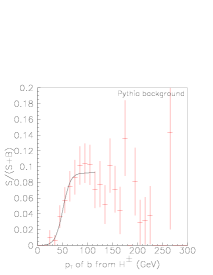
Figure 84: Bin by bin values of $S/(S+B)$ for the $p_{T}$ of the $b$–tagged jet, considered to come from the $H^{\pm}\to tb$ decay. $S$ and $B$ are the numbers of events for signal and background respectively. ($30\,\mathrm{fb}^{-1}$, $m_{A}=300\,\mathrm{GeV}$, $\tan\beta=50$)

Figure 85: Sum of the leptonic and hadronic solutions of the charged Higgs boson mass for the signal, the background and the sum of the background and the signal. ($m_{A}=300\,\mathrm{GeV}$, $\tan\beta=50$, $30\,\mathrm{fb}^{-1}$)

3.5.2 Signal significance and discovery contours

The discovery potential for this analysis at low luminosity in the CMS experiment has been estimated, using the statistical significance of the signal defined as $\sigma=S/\sqrt{B}$, with $S$ and $B$ the number of signal and background events respectively. Discovery contours have been constructed in the MSSM parameter space for $\sigma=5$. For an integrated luminosity of $30\,\mathrm{fb}^{-1}$ and $60\,\mathrm{fb}^{-1}$, the result is shown in Fig. 87, using the $t\bar{t}$ background. In the same plot, also the current discovery contour is shown for the subdominant decay channel, $H^{\pm}\to\tau\nu$, after $30\mathrm{fb}^{-1}$ of integrated luminosity [450]. The large difference with the previous CMS result [440] was found to be due to the large drop in the prediction of the signal cross section, described in Section 3.2 In Fig. 87 the comparison is shown of the LO $t\bar{t}$ background with the NLO result, and with the LO $t\bar{t}b/t\bar{t}j$ background, for $30\,\mathrm{fb}^{-1}$.

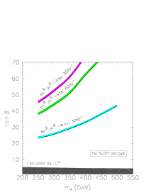
Figure 86: Discovery contours for the $tH^{\pm},H^{\pm}\to tb$ channel with $30\,\mathrm{fb}^{-1}$ and $60\,\mathrm{fb}^{-1}$, and for the $tH^{\pm},H^{\pm}\to\tau\nu$ channel with $30\,\mathrm{fb}^{-1}$.

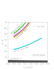
Figure 87: Discovery contours for the $tH^{\pm},H^{\pm}\to tb$ channel with $30\,\mathrm{fb}^{-1}$, for the backgrounds $t\bar{t}$ from PYTHIA at LO and NLO, and $t\bar{t}b/t\bar{t}j$ from MadGraph/MadEvent at LO.

3.5.3 Influence of systematic uncertainties on the background cross section

So far in this study, the significance has been calculated in the ideal case of perfect knowledge of the background cross section. The background is large, however, and the combinatorial background limits the analysis to a counting experiment. Therefore, the effect of systematical uncertainties on the knowledge of the background has been estimated.

Two methods are proposed to extract the background from data. First, the difference between the signal and the background for the $p_{T}$ spectrum of the $b$-jet from the Higgs decay was used, looking at the low $p_{T}$ region. The background can in this way be measured with an uncertainty of about 5% from statistics and remaining signal, plus an additional, possibly sizeable, contribution from the uncertainty on the shape of this $p_{T}$ distribution. Another possibility is the measurement of the background, tagging 1 $b$–jet less. Using a measured $b$–tagging efficiency and purity, one can then calculate the background when tagging three $b$–jets. A 7% systematic uncertainty was estimated this way, due to the uncertainty on the $b$–mistag probability, which was taken as 10%, as found as systematical uncertainty in CDF for the secondary vertex tag technique [451]. Additionally, a possibly sizeable uncertainty is introduced from the ratio of $t\bar{t}b$ to $t\bar{t}j$ events.

In the absence of an experimental measurement of the background, it can be estimated from the theoretically calculated cross section, the luminosity and the reconstruction and analysis efficiencies. One should then add a typical 10 to 15% uncertainty from the not yet available NLO calculation, an expected 5% from the luminosity measurement, and additional contributions from the event selection.

With these systematical uncertainty estimations, the effects on the visibility of the signal can be evaluated. Considering a systematical uncertainty of $\epsilon B$ background events after full analysis, a total uncertainty $\Delta B=\sqrt{B+\epsilon^{2}B^{2}}$ on the number of background events $B$ is obtained. The signal significance for $S$ signal events now becomes $\sigma=S/\sqrt{B+\epsilon^{2}B^{2}}$. For this channel with large background, the $S/B$ value is small, and cannot be improved without losing too much signal statistics. In Fig. 88 the discovery contours are plotted, when supposing perfect knowledge of the $t\bar{t}$ cross section ($\epsilon=0$), a $1\%$ ($\epsilon=0.01$) and a $3\%$ uncertainty ($\epsilon=0.03$). A value of $5\%$ doesn’t show up anymore on the plot.

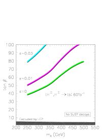
Figure 88: Influence on the discovery contour of systematical uncertainties $\epsilon$ ($0\%$, $1\%$ and $3\%$) on the $t\bar{t}$ background, for $60\,\mathrm{fb}^{-1}$.

3.6 Fully Hadronic Channel

The fully hadronic $tH^{\pm}\to ttb$ decay, where both $W^{\pm}$’s from the $t$ decay hadronically, has also been studied. In this case there is no lepton to trigger on, however, and it was found that the CMS jet trigger acceptances at HLT alone, already reduce the signal to 1 to 7% for $250\,\mathrm{GeV}<m_{A}<500\,\mathrm{GeV}$. Without an HLT $b$–trigger, no hope is left for this decay channel.

3.7 Conclusion

In this paper the prospects have been presented to discover, in CMS at low luminosity, a heavy charged MSSM Higgs boson in the $H^{\pm}\to tb$ decay channel, asking for three $b$–tagged jets. The latest signal cross section values were used, along with a matrix element simulation of the $t\bar{t}b/t\bar{t}j$ background. This analysis includes HLT acceptances. The background was rejected with a factor 2 600, while the signal efficiency ranged from 0.6% to 1.0% for $250\,\mathrm{GeV}<m_{A}<500\,\mathrm{GeV}$. Discovery contours were constructed, and the effects of systematic uncertainties on the background were investigated. An uncertainty $\epsilon$ of at least 10% on the background level was estimated, starting from data or theoretical calculations. For $\epsilon=0.03$, however, the reach is limited to $\tan\beta>80$. Therefore, no visibility for this channel is left in the MSSM parameter space.

J. NMSSM Higgs Discovery at the LHC
U. Ellwanger, J.F. Gunion, C. Hugonie and S. Moretti

1 Introduction

One of the most attractive supersymmetric models is the Next to Minimal Supersymmetric Standard Model (NMSSM) (see [452, 453] and references therein) which extends the MSSM by the introduction of just one singlet superfield, $\widehat{S}$. When the scalar component of $\widehat{S}$ acquires a TeV scale vacuum expectation value (a very natural result in the context of the model), the superpotential term $\widehat{S}\widehat{H}_{u}\widehat{H}_{d}$ generates an effective $\mu\widehat{H}_{u}\widehat{H}_{d}$ interaction for the Higgs doublet superfields. Such a term is essential for acceptable phenomenology. No other SUSY model generates this crucial component of the superpotential in as natural a fashion. Thus, the phenomenological implications of the NMSSM at future accelerators should be considered very seriously. One aspect of this is the fact that the $h,H,A,H^{\pm}$ Higgs sector of the MSSM is extended so that there are three CP-even Higgs bosons ($h_{1,2,3}$, $m_{h_{1}}<m_{h_{2}}<m_{h_{3}}$), two CP-odd Higgs bosons ($a_{1,2}$, $m_{a_{1}}<m_{a_{2}}$) (we assume that CP is not violated in the Higgs sector) and a charged Higgs pair ($h^{\pm}$). An important question is then the extent to which the no-lose theorem for MSSM Higgs boson discovery at the LHC (after LEP constraints) is retained when going to the NMSSM; i.e. is the LHC guaranteed to find at least one of the $h_{1,2,3}$, $a_{1,2}$, $h^{\pm}$? The first exploration of this issue appeared in [454], with the conclusion that for substantial portions of parameter space the LHC would be unable to detect any of the NMSSM Higgs bosons. Since then, there have been improvements in many of the detection modes and the addition of new ones. These will be summarized below and the implications reviewed. However, these improvements and additions do not address the possibly important $h\to aa$ type decays that could suppress all other types of signals [454, 455].

One of the key ingredients in the no-lose theorem for MSSM Higgs boson discovery is the fact that relations among the Higgs boson masses are such that decays of the SM-like Higgs boson to $AA$ are only possible if $m_{A}$ is quite small, a region that is ruled out by LEP by virtue of the fact that $Z\to hA$ pair production was not detected despite the fact that the relevant coupling is large for small $m_{A}$. In the NMSSM, the lighter Higgs bosons, $h_{1}$ or $h_{2}$, can be SM-like (in particular being the only Higgs with substantial $WW/ZZ$ coupling) without the $a_{1}$ necessarily being heavy. In addition, this situation is not excluded by LEP searches for $e^{+}e^{-}\to Z^{*}\to h_{1,2}a_{1}$ since, in the NMSSM, the $a_{1}$ can have small $Zh_{2}a_{1}$ ($Zh_{1}a_{1}$) coupling when $h_{1}$ ($h_{2}$) is SM-like. [In addition, sum rules require that the $Zh_{1}a_{1}$ ($Zh_{2}a_{1}$) coupling is small when the $h_{1}WW$ ($h_{2}WW$) couplings are near SM strength.] As a result, NMSSM parameters that are not excluded by current data can be chosen so that the $h_{1,2}$ masses are moderate in size ($\sim 100-130$ GeV) and the $h_{1}\to a_{1}a_{1}$ or $h_{2}\to a_{1}a_{1}$ decays are dominant. Dominance of such decays falls outside the scope of the usual detection modes for the SM-like MSSM $h$ on which the MSSM no-lose LHC theorem largely relies.

In Ref. [453], a partial no-lose theorem for NMSSM Higgs boson discovery at the LHC was established. In particular, it was shown that the LHC would be able to detect at least one of the Higgs bosons (typically, one of the lighter CP-even Higgs states) throughout the full parameter space of the model, excluding only those parameter choices for which there is sensitivity to the model-dependent decays of Higgs bosons to other Higgs bosons and/or superparticles. Here, we will address the question of whether or not this no-lose theorem can be extended to those regions of NMSSM parameter space for which Higgs bosons can decay to other Higgs bosons. We find that the parameter choices such that the “standard” discovery modes fail would allow Higgs boson discovery if detection of $h\to aa$ decays is possible. (When used generically, the symbol $h$ will now refer to $h=h_{1}$, $h_{2}$ or $h_{3}$ and the symbol $a$ will refer to $a=a_{1}$ or $a_{2}$). Detection of $h\to aa$ will be difficult since each $a$ will decay primarily to $b\overline{b}$ (or 2 jets if $m_{a}<2m_{b}$), $\tau^{+}\tau^{-}$, and, possibly, $\widetilde{\chi}_{1}^{0}\widetilde{\chi}_{1}^{0}$, yielding final states that will typically have large backgrounds at the LHC.

In [453] we scanned the parameter space, removing parameter choices ruled out by constraints from LEP on Higgs boson production, $e^{+}e^{-}\to Zh$ or $e^{+}e^{-}\to ha$ [456], and eliminating parameter choices for which one Higgs boson can decay to two other Higgs bosons or a vector boson plus a Higgs boson. For the surviving regions of parameter space, we estimated the statistical significances ($N_{SD}=S/\sqrt{B}$) for all Higgs boson detection modes so far studied at the LHC [457, 59, 77, 78]. These are (with $\ell=e,\mu$)

1) $gg\to h/a\to\gamma\gamma$;

2) associated $Wh/a$ or $t\bar{t}h/a$ production with $\gamma\gamma\ell^{\pm}$ in the final state;

3) associated $t\bar{t}h/a$ production with $h/a\to b\bar{b}$;

4) associated $b\bar{b}h/a$ production with $h/a\to\tau^{+}\tau^{-}$;

5) $gg\to h\to ZZ^{(*)}\to$ 4 leptons;

6) $gg\to h\to WW^{(*)}\to\ell^{+}\ell^{-}\nu\bar{\nu}$;

7) $WW\to h\to\tau^{+}\tau^{-}$;

8) $WW\to h\to WW^{(*)}$.

For an integrated luminosity of $300~{}{\rm fb}^{-1}$ at the LHC, all the surviving points yielded $N_{SD}>10$ after combining all modes, including the $W$-fusion modes. Thus, NMSSM Higgs boson discovery by just one detector with $L=300~{}{\rm fb}^{-1}$ is essentially guaranteed for those portions of parameter space for which Higgs boson decays to other Higgs bosons or supersymmetric particles are kinematically forbidden.

In this work, we investigate the complementary part of the parameter space, where at least one Higgs boson decays to other Higgs bosons. To be more precise, we require at least one of the following decay modes to be kinematically allowed:

$$i)\ h\to h^{\prime}h^{\prime}\;,\quad ii)\ h\to aa\;,\quad iii)\ h\to h^{\pm}h^{\mp}\;,\quad iv)\ h\to aZ\;,$$

$$v)\ h\to h^{\pm}W^{\mp}\;,\quad vi)\ a^{\prime}\to ha\;,\quad vii)\ a\to hZ\;,\quad viii)\ a\to h^{\pm}W^{\mp}\;.$$ (74)

After searching those regions of parameter space for which one or more of the decays $i)-viii)$ is allowed, we found that the only subregions for which discovery of a Higgs boson in modes 1) – 8) was not possible correspond to NMSSM parameter choices for which (a) there is a light CP-even Higgs boson with substantial doublet content that decays mainly to two still lighter CP-odd Higgs states, $h\to aa$, and (b) all the other Higgs states are either dominantly singlet-like, implying highly suppressed production rates, or relatively heavy, decaying to $t\overline{t}$, to one of the “difficult” modes $i)-viii)$ or to a pair of sparticles. In such cases, the best opportunity for detecting at least one of the NMSSM Higgs bosons is to employ $WW\to h$ production and develop techniques for extracting a signal for the $h\to aa\to jj\tau^{+}\tau^{-}$ (including $jj=b\overline{b}$) process. We have performed a detailed simulation of the $aa\to jj\tau^{+}\tau^{-}$ final state and find that its detection may be possible after accumulating $300~{}{\rm fb}^{-1}$ in both the ATLAS and CMS detectors.

2 The model and scanning procedures

We consider the simplest version of the NMSSM [452], where the term $\mu\widehat{H}_{1}\widehat{H}_{2}$ in the superpotential of the MSSM is replaced by (we use the notation $\widehat{A}$ for the superfield and $A$ for its scalar component field)

$$\lambda\widehat{H}_{1}\widehat{H}_{2}\widehat{S}\ +\ \frac{\kappa}{3}\widehat{S}^{3}\ \ ,$$ (75)

so that the superpotential is scale invariant. We make no assumption on “universal” soft terms. Hence, the five soft supersymmetry breaking terms

$$m_{H_{1}}^{2}H_{1}^{2}\ +\ m_{H_{2}}^{2}H_{2}^{2}\ +\ m_{S}^{2}S^{2}\ +\ \lambda A_{\lambda}H_{1}H_{2}S\ +\ \frac{\kappa}{3}A_{\kappa}S^{3}$$ (76)

are considered as independent. The masses and/or couplings of sparticles will be such that their contributions to the loop diagrams inducing Higgs boson production by gluon fusion and Higgs boson decay into $\gamma\gamma$ are negligible. In the gaugino sector, we chose $M_{2}=1~{}{\rm TeV}$ (at low scales). Assuming universal gaugino masses at the coupling constant unification scale, this yields $M_{1}\sim 500~{}{\rm GeV}$ and $M_{3}\sim 3~{}{\rm TeV}$. In the squark sector, as particularly relevant for the top squarks which appear in the radiative corrections to the Higgs potential, we chose the soft masses $m_{Q}=m_{T}\equiv M_{susy}=1$ TeV, and varied the stop mixing parameter

$$X_{t}\equiv 2\ \frac{A_{t}^{2}}{M_{susy}^{2}+m_{t}^{2}}\left(1-\frac{A_{t}^{2}}{12(M_{susy}^{2}+m_{t}^{2})}\right)\ .$$ (77)

As in the MSSM, the value $X_{t}=\sqrt{6}$ – so called maximal mixing – maximizes the radiative corrections to the Higgs boson masses, and we found that it leads to the most challenging points in the parameter space of the NMSSM. We adopt the convention $\lambda,\kappa>0$, in which $\tan\beta$ can have either sign. We require $|\mu_{\rm eff}|\ >\ 100$ GeV; otherwise a light chargino would have been detected at LEP. The only possibly light SUSY particle will be the $\widetilde{\chi}_{1}^{0}$. A light $\widetilde{\chi}_{1}^{0}$ is a frequent characteristic of parameter choices that yield a light $a_{1}$.

We have performed a numerical scan over the free parameters. For each point, we computed the masses and mixings of the CP-even and CP-odd Higgs bosons, $h_{i}$ ($i=1,2,3$) and $a_{j}$ ($j=1,2$), taking into account radiative corrections up to the dominant two loop terms, as described in [458]. We eliminated parameter choices excluded by LEP constraints [456] on $e^{+}e^{-}\to Zh_{i}$ and $e^{+}e^{-}\to h_{i}a_{j}$. The latter provides an upper bound on the $Zh_{i}a_{j}$ reduced coupling, $R^{\prime}_{ij}$, as a function of $m_{h_{i}}+m_{a_{j}}$ for $m_{h_{i}}\simeq m_{a_{j}}$. Finally, we calculated $m_{h^{\pm}}$ and required $m_{h^{\pm}}>155$ GeV, so that $t\to h^{\pm}b$ would not be seen.

In order to probe the complementary part of the parameter space as compared to the scanning of Ref. [453], we required that at least one of the decay modes $i)-viii)$ is allowed. For each Higgs state, we calculated all branching ratios including those for modes $i)-viii)$, using an adapted version of the FORTRAN code HDECAY [165]. We then estimated the expected statistical significances at the LHC in all Higgs boson detection modes 1) – 8) by rescaling results for the SM Higgs boson and/or the MSSM $h,H$ and/or $A$. The rescaling factors are determined by $R_{i}$, $t_{i}$ and $b_{i}=\tau_{i}$, the ratios of the $VVh_{i}$, $t\overline{t}h_{i}$ and $b\overline{b}h_{i},\tau^{+}\tau^{-}h_{i}$ couplings, respectively, to those of a SM Higgs boson. Of course $|R_{i}|<1$, but $t_{i}$ and $b_{i}$ can be larger, smaller or even differ in sign with respect to the SM. For the CP-odd Higgs bosons, $R_{i}^{\prime}=0$ at tree-level; $t^{\prime}_{j}$ and $b^{\prime}_{j}$ are the ratios of the $i\gamma_{5}$ couplings for $t\bar{t}$ and $b\bar{b}$, respectively, relative to SM-like strength. A detailed discussion of the procedures for rescaling SM and MSSM simulation results for the statistical significances in channels 1) – 8) will appear elsewhere.

Point Number	1	2	3	4	5	6
Bare Parameters
$\lambda$	0.2872	0.2124	0.3373	0.3340	0.4744	0.5212
$\kappa$	0.5332	0.5647	0.5204	0.0574	0.0844	0.0010
$\tan\beta$	2.5	3.5	5.5	2.5	2.5	2.5
$\mu_{\rm eff}~{}({\rm GeV})$	200	200	200	200	200	200
$A_{\lambda}~{}({\rm GeV})$	100	0	50	500	500	500
$A_{\kappa}~{}({\rm GeV})$	0	0	0	0	0	0
CP-even Higgs Boson Masses and Couplings
$m_{h_{1}}$ (GeV)	115	119	123	76	85	51
$R_{1}$	1.00	1.00	-1.00	0.08	0.10	-0.25
$t_{1}$	0.99	1.00	-1.00	0.05	0.06	-0.29
$b_{1}$	1.06	1.05	-1.03	0.27	0.37	0.01
Relative gg Production Rate	0.97	0.99	0.99	0.00	0.01	0.08
$BR(h_{1}\to b\overline{b})$	0.02	0.01	0.01	0.91	0.91	0.00
$BR(h_{1}\to\tau^{+}\tau^{-})$	0.00	0.00	0.00	0.08	0.08	0.00
$BR(h_{1}\to a_{1}a_{1})$	0.98	0.99	0.98	0.00	0.00	1.00
$m_{h_{2}}$ (GeV)	516	626	594	118	124	130
$R_{2}$	-0.03	-0.01	0.01	-1.00	-0.99	-0.97
$t_{2}$	-0.43	-0.30	-0.10	-0.99	-0.99	-0.95
$b_{2}$	2.46	-3.48	3.44	-1.03	-1.00	-1.07
Relative gg Production Rate	0.18	0.09	0.01	0.98	0.99	0.90
$BR(h_{2}\to b\overline{b})$	0.01	0.04	0.04	0.02	0.01	0.00
$BR(h_{2}\to\tau^{+}\tau^{-})$	0.00	0.01	0.00	0.00	0.00	0.00
$BR(h_{2}\to a_{1}a_{1})$	0.04	0.02	0.83	0.97	0.98	0.96
$m_{h_{3}}$ (GeV)	745	1064	653	553	554	535
CP-odd Higgs Boson Masses and Couplings
$m_{a_{1}}$ (GeV)	56	7	35	41	59	7
$t_{1}^{\prime}$	0.05	0.03	0.01	-0.03	-0.05	-0.06
$b_{1}^{\prime}$	0.29	0.34	0.44	-0.20	-0.29	-0.39
Relative gg Production Rate	0.01	0.03	0.05	0.01	0.01	0.05
$BR(a_{1}\to b\overline{b})$	0.92	0.00	0.93	0.92	0.92	0.00
$BR(a_{1}\to\tau^{+}\tau^{-})$	0.08	0.94	0.07	0.07	0.08	0.90
$m_{a_{2}}$ (GeV)	528	639	643	560	563	547
Charged Higgs Mass (GeV)	528	640	643	561	559	539
Most Visible of the LHC Processes 1)-8)	2 ($h_{1}$)	2 ($h_{1}$)	8 ($h_{1}$)	2 ($h_{2}$)	8 ($h_{2}$)	8 ($h_{2}$)
$N_{SD}=S/\sqrt{B}$ Significance of this process at $L=$300 ${\rm fb}^{-1}$	0.48	0.26	0.55	0.62	0.53	0.16
$N_{SD}(L=300~{}{\rm fb}^{-1})$ for $WW\to h\to aa\to jj\tau^{+}\tau^{-}$ at LHC	50	22	69	63	62	21

Table 29: Properties of selected scenarios that could escape detection at the LHC. In the table, $R_{i}=g_{h_{i}VV}/g_{h_{SM}VV}$, $t_{i}=g_{h_{i}t\overline{t}}/g_{h_{SM}t\overline{t}}$ and $b_{i}=g_{h_{i}b\overline{b}}/g_{h_{SM}b\overline{b}}$ for $m_{h_{SM}}=m_{h_{i}}$; $t_{1}^{\prime}$ and $b_{1}^{\prime}$ are the $i\gamma_{5}$ couplings of $a_{1}$ to $t\overline{t}$ and $b\overline{b}$ normalized relative to the scalar $t\overline{t}$ and $b\overline{b}$ SM Higgs couplings. We also give the $gg$ fusion production rate ratio, $gg\to h_{i}/gg\to h_{SM}$, for $m_{h_{SM}}=m_{h_{i}}$. Important absolute branching ratios are displayed. For points 2 and 6, the decays $a_{1}\to jj$ ($j\neq b$) have $BR(a_{1}\to jj)\simeq 1-BR(a_{1}\to\tau^{+}\tau^{-})$. For the heavy $h_{3}$ and $a_{2}$, we give only their masses. For all points 1 – 6, the statistical significances for the detection of any Higgs boson in any of the channels 1) – 8) are tiny; the next-to-last row gives their maximum together with the process number and the corresponding Higgs state. The last row gives the statistical significance of the new $WW\to h\to aa\to jj\tau^{+}\tau^{-}$ [$h=h_{1}$ ($h=h_{2}$) for points 1–3 (4–6)] LHC signal explored here.

In our set of randomly scanned points, we selected those for which all the statistical significances in modes 1) – 8) are below $5\sigma$. We obtained a lot of points, all with similar characteristics. Namely, in the Higgs spectrum, we always have a very SM-like CP-even Higgs boson with a mass between 115 and 135 GeV (i.e. above the LEP limit), which can be either $h_{1}$ or $h_{2}$, with a reduced coupling to the gauge bosons $R_{1}\simeq 1$ or $R_{2}\simeq 1$, respectively. This state decays dominantly to a pair of (very) light CP-odd states, $a_{1}a_{1}$, with $m_{a_{1}}$ between 5 and 65 GeV. The singlet component of $a_{1}$ cannot be dominant if we are to have a large $h_{1}\to a_{1}a_{1}$ or $h_{2}\to a_{1}a_{1}$ branching ratio when the $h_{1}$ or $h_{2}$, respectively, is the SM-like Higgs boson. Further, when the $h_{1}$ or $h_{2}$ is very SM-like, one has small $Zh_{1}a_{1}$ or $Zh_{2}a_{1}$ coupling, respectively, so that $e^{+}e^{-}\to h_{1}a_{1}$ or $e^{+}e^{-}\to h_{2}a_{1}$ associated production places no constraint on the light CP-odd state at LEP. We have selected six difficult benchmark points, displayed in Table 29. These are such that $a_{1}\to\widetilde{\chi}_{1}^{0}\widetilde{\chi}_{1}^{0}$ decays are negligible or forbidden. (Techniques for cases such that $\widetilde{\chi}_{1}^{0}\widetilde{\chi}_{1}^{0}$ decay modes are important are under development.) For points 1 – 3, $h_{1}$ is the SM-like CP-even state, while for points 4 – 6 it is $h_{2}$. We have selected the points so that there is some variation in the $h_{1,2}$ and $a_{1}$ masses. The main characteristics of the benchmark points are displayed in Table 29. Note the large $BR(h\to a_{1}a_{1})$ of the SM-like $h$ ($h=h_{1}$ for points 1 – 3 and $h=h_{2}$ for points 4 –6). For points 4 – 6, with $m_{h_{1}}<100~{}{\rm GeV}$, the $h_{1}$ is mainly singlet. As a result, the $Zh_{1}a_{1}$ coupling is very small, implying no LEP constraints on the $h_{1}$ and $a_{1}$ from $e^{+}e^{-}\to h_{1}a_{1}$ production.

We note that in the case of the points 1 – 3, the $h_{2}$ would not be detectable either at the LHC or at a Linear Collider (LC). For points 4 – 6, the $h_{1}$, though light, is singlet in nature and would not be detectable. Further, the $h_{3}$ or $a_{2}$ will only be detectable for points 1 – 6 if a super high energy LC is eventually built so that $e^{+}e^{-}\to Z\to h_{3}a_{2}$ is possible. Thus, we will focus on searching for the SM-like $h_{1}$ ($h_{2}$) for points 1 – 3 (4 – 6) using the dominant $h_{1}(h_{2})\to a_{1}a_{1}$ decay mode.

In the case of points 2 and 6, the $a_{1}\to\tau^{+}\tau^{-}$ decays are dominant. The final state of interest will be $jj\tau^{+}\tau^{-}$, where the $jj$ actually comes primarily from $a_{1}a_{1}\to\tau^{+}\tau^{-}\tau^{+}\tau^{-}$ followed by jet decays of two of the $\tau$’s: $\tau^{+}\tau^{-}\to jj+\nu^{\prime}s$. (The contribution from direct $a_{1}\to jj$ decays to the $jj\tau^{+}\tau^{-}$ final state is relatively small for points 2 and 6.) In what follows, when we speak of $\tau^{+}\tau^{-}$, we refer to those $\tau$’s that are seen in the $\tau^{+}\tau^{-}\to\ell^{+}\ell^{-}+\nu^{\prime}s$ final state ($\ell=e,\mu$). For points 1 and 3 – 5 $BR(a_{1}\to b\overline{b})$ is substantial. The relevant final state is $b\overline{b}\tau^{+}\tau^{-}$. Nonetheless, we begin with a study of the backgrounds and signals without requiring $b$-tagging. With our latest cuts, we will see that $b$-tagging is not necessary to overcome the apriori large Drell-Yan $\tau^{+}\tau^{-}$+jets background. It is eliminated by stringent cuts for finding the highly energetic forward / backward jets characteristic of the $WW$ the fusion process. As a result, we will find good signals for all 6 of our points.

In principle, one could explore final states other than $b\overline{b}\tau^{+}\tau^{-}$ (or $jj\tau^{+}\tau^{-}$ for points 2 and 6). However, all other channels will be much more problematical at the LHC. A $4b$-signal would be burdened by a large QCD background even after implementing $b$-tagging. A $4j$-signal would be completely swamped by QCD background. Meanwhile, the $4\tau$-channel (by which we mean that all taus decay leptonically) would not allow one to reconstruct the $h_{1},h_{2}$ resonances.

In the case of the $2b2\tau$ (or $2j2\tau$) signature, we identify the $\tau$’s through their leptonic decays to electrons and muons. Thus, they will yield some amount of missing (transverse) momentum, $p_{\rm miss}^{T}$. This missing transverse momentum can be projected onto the visible $e,\mu$-momenta in an attempt to reconstruct the parent $\tau$-direction.

3 Monte Carlo Results for the LHC

Let us now focus on the $WW\to h\to aa$ channel that we believe provides the best hope for Higgs detection in these difficult NMSSM cases. (We reemphasize that the $h_{1}$ [cases 1 – 3] or $h_{2}$ [cases 4 – 6] has nearly full SM strength coupling to $WW$.) The $b\overline{b}\tau^{+}\tau^{-}$ (or $2j\tau^{+}\tau^{-}$, for points 2 and 6) final state of relevance is complex and subject to large backgrounds, and the $a_{1}$ masses of interest are very modest in size. In order to extract the $WW$ fusion $2j2\tau$ NMSSM Higgs boson signature, it is crucial to strongly exploit forward and backward jet tagging on the light quarks emerging after the double $W$-strahlung preceding $WW$-fusion. We also require two additional central jets (from one of the $a$’s) and two opposite sign central leptons ($\ell=e,\mu$) coming from the the $\tau^{+}\tau^{-}$ emerging from the decay of the other $a$. By imposing stringent forward / backward jet tagging cuts, we remove the otherwise very large background from Drell-Yan $\tau^{+}\tau^{-}+jets$ production. In the end, the most important background is due to $t\overline{t}$ production and decay via the purely SM process, $gg\to t\bar{t}\to b\bar{b}W^{+}W^{-}\to b\bar{b}\tau^{+}\tau^{-}+p_{\rm miss}^{T},$ in association with forward and backward jet radiation.

We have employed numerical simulations based on a version of HERWIG v6.4 [296, 395, 294] modified to allow for appropriate NMSSM couplings and decay rates. Calorimeter emulation was performed using the GETJET code [459]. Since the $a_{1}$ will not have been detected previously, we must assume a value for $m_{a_{1}}$. In dealing with actual experimental data, it will be necessary to repeat the analysis for densely spaced $m_{a_{1}}$ values and look for the $m_{a_{1}}$ choice that produces the best signal. We look among the central jets for the combination with invariant mass $M_{jj}$ closest to $m_{a_{1}}$. In Fig. 89, we show the $M_{jj\tau^{+}\tau^{-}}$ invariant mass distribution obtained after cuts, but before $b$-tagging or inclusion of $K$ factors — the plot presented assumes that we have hit on the correct $m_{a_{1}}$ choice.

               LHC, $\sqrt{s_{pp}}=14$ TeV

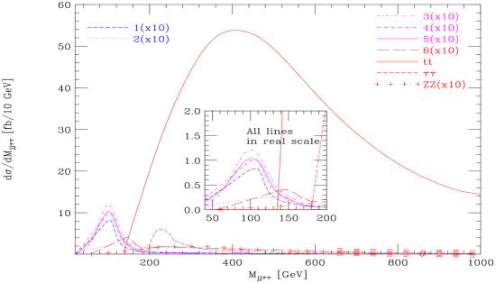
Figure 89: We plot $d\sigma/dM_{jj\tau^{+}\tau^{-}}$ [fb/10 GeV] vs $M_{jj\tau^{+}\tau^{-}}$ [GeV] for signals and backgrounds after basic event selections, but before $b$ tagging. The lines corresponding to points 4 and 5 are visually indistinguishable. No $K$ factors are included.

The selection strategy adopted is a more refined (as regards forward / backward jet tagging) version of that summarized in [460]. It is clearly efficient in reconstructing the $h_{1}$ (for points 1–3) and $h_{2}$ (for points 4–6) masses from the $jj\tau^{+}\tau^{-}$ system, as one can appreciate by noting the peaks appearing at $M_{jj\tau^{+}\tau^{-}}\approx 100$ GeV. In contrast, the heavy Higgs resonances at $m_{h_{2}}$ for points 1–3 and the rather light resonances at $m_{h_{1}}$ for points 4–6 (recall Table 29) do not appear, the former mainly because of the very poor production rates and the latter due to the fact that either the $h_{1}\to a_{1}a_{1}$ decay mode is not open (points 4, 5) or – if it is – the jets and $e/\mu$-leptons eventually emerging from the $a_{1}$ decays are too soft to pass the acceptance cuts (point 6, for which $m_{a_{1}}=7$ GeV and $m_{h_{1}}=51$ GeV). For all six NMSSM setups, the Higgs resonance produces a bump below the end of the low mass tail of the $t\bar{t}$ background (see the insert in Fig. 89). Note how small the DY $\tau^{+}\tau^{-}$ background is after strong forward / backward jet tagging. Since the main surviving background is from $t\overline{t}$ production, $b$ tagging is not helpful. For points 2 and 6, for which the signal has no $b$’s in the final state, anti-$b$-tagging might be useful, but has not been considered here.

To estimate $S/\sqrt{B}$, we assume $L=300~{}{\rm fb}^{-1}$, a $K$ factor of 1.1 for the $WW$ fusion signal and $K$ factors of 1, 1 and 1.6 for the DY $\tau^{+}\tau^{-}$, $ZZ$ production and $t\overline{t}$ backgrounds, respectively. (These $K$ factors are not included in the plot of Fig. 89.) We sum events over the region $40\leq M_{jj\tau^{+}\tau^{-}}\leq 150$ GeV. (Had we only included masses below $130$ GeV, we would have had no $t\overline{t}$ background, and the $S/\sqrt{B}$ values would be enormous. However, we are concerned that this absence of $t\overline{t}$ background below $130~{}{\rm GeV}$ might be a reflection of limited Monte Carlo statistics. As a result we have taken the more conservative approach of at least including the first few bins for which our Monte Carlo does predict some $t\overline{t}$ background.)

For points 1, 2, 3, 4, 5 and 6, we obtain signal rates of about $S=1636$, 702, 2235, 2041, 2013, and 683, respectively. The $t\overline{t}$+jets background rate is $B_{tt}\sim 795$. The $ZZ$ background rate is $B_{ZZ}\sim 6$. The DY $\tau^{+}\tau^{-}$ background rate is negligible. (We are continuing to increase our statistics to get a fully reliable estimate.) The resulting $N_{SD}=S/\sqrt{B}$ values for points 1-6 are 50, 22, 69, 63, 62, and 21, respectively. The smaller values for points 2 and 6 are simply a reflection of the difficulty of isolating and reconstructing the two jets coming from the decay of a very light $a_{1}$. Overall, these preliminary results are very encouraging and suggest that a no-lose theorem for NMSSM Higgs detection at the LHC is close at hand.

4 Conclusions

In summary, we have obtained a statistically very significant LHC signal in the $jj\tau^{+}\tau^{-}$ final state of $WW$ fusion for cases in which the NMSSM parameters are such that the most SM-like of the CP-even Higgs bosons, $h$, is relatively light and decays primarily to a pair of CP-odd Higgs states, $h\to aa$ with $a\to b\overline{b},\tau^{+}\tau^{-}$ if $m_{a}>2m_{b}$ or $a\to jj,\tau^{+}\tau^{-}$ if $m_{a}<2m_{b}$. The statistical significances are (at least) of order 50 to 70 for points with $m_{a}>2m_{b}$ and of order 20 for points with $m_{a}<2m_{b}$. These high significances were obtained by imposing stringent cuts requiring highly energetic forward / backward jets in order to isolate the $WW$ fusion signal process from backgrounds such as DY $\tau^{+}\tau^{-}$ pair production. Still, this signal will be the only evidence for Higgs bosons at the LHC. A future LC will probably be essential in order to confirm that the enhancement seen at the LHC really does correspond to a Higgs boson. At the LC, discovery of a light SM-like $h$ is guaranteed to be possible in the $Zh$ final state using the recoil mass technique [461].

In the present study, we have not explored the cases in which the $a_{1}\to\widetilde{\chi}_{1}^{0}\widetilde{\chi}_{1}^{0}$ decay has a large branching ratio. Detecting a Higgs signal in such cases will require a rather different procedure. Work on the $WW\to h\to{\rm invisible}$ signal is in progress [462].

As we have stressed, for parameter space points of the type we have discussed here, detection of any of the other MSSM Higgs bosons is likely to be impossible at the LHC and is likely to require an LC with $\sqrt{s_{e^{+}e^{-}}}$ above the relevant thresholds for $h^{\prime}a^{\prime}$ production, where $h^{\prime}$ and $a^{\prime}$ are heavy CP-even and CP-odd Higgs bosons, respectively.

Although results for the LHC indicate that Higgs boson discovery will be possible for the type of situations we have considered, it is clearly important to refine and improve the techniques for extracting a signal. This will almost certainly be possible once data is in hand and the $t\overline{t}$ background can be more completely modeled.

Clearly, if SUSY is discovered and $WW\to WW$ scattering is found to be perturbative at $WW$ energies of 1 TeV (and higher), and yet no Higgs bosons are detected in the standard MSSM modes, a careful search for the signal we have considered should have a high priority.

Finally, we should remark that the $h\to aa$ search channel considered here in the NMSSM framework is also highly relevant for a general two-Higgs-doublet model, 2HDM. It is really quite possible that the most SM-like CP-even Higgs boson of a 2HDM will decay primarily to two CP-odd states. This is possible even if the CP-even state is quite heavy, unlike the NMSSM cases considered here. If CP violation is introduced in the Higgs sector, either at tree-level or as a result of one-loop corrections (as, for example, is possible in the MSSM), $h\to h^{\prime}h^{\prime\prime}$ decays will generally be present. The critical signal will be the same as that considered here.

K. Higgs Coupling Measurements at a 1 TeV Linear Collider
T. Barklow

1 Introduction

The precision measurement of the Higgs boson couplings to fermions and gauge bosons is one of the most important goals of an $e^{+}e^{-}$ linear collider. These measurements will distinguish between different models of electroweak symmetry breaking, and can be used to extract parameters within a specific model, such as supersymmetry. Most linear collider Higgs studies have been made assuming a center-of-mass energy of 0.35 TeV, where the Higgsstrahlung cross-section is not too far from its peak value for Higgs boson masses less than 250 GeV . Higgs branching fraction measurements with errors of $2-10$% can be achieved at $\sqrt{s}=0.35$ TeV for many Higgs decay modes, and the total Higgs width can be measured with an accuracy of $5-13$% if the $\sqrt{s}=0.35$ TeV data is combined with $WW$ fusion production at $\sqrt{s}=0.50$ TeV[316]. These measurement errors are very good, but is it possible to do better?

In the CLIC study of physics at a 3 TeV $e^{+}e^{-}$ linear collider it was recognized that rare Higgs decay modes such as $h\rightarrow\mu^{+}\mu^{-}$ could be observed using Higgs bosons produced through $WW$ fusion[463, 464]. This is possible because the cross-section for Higgs production through $WW$ fusion rises with center-of-mass energy, while the design luminosity of a linear collider also rises with energy. One doesn’t have to wait for a center-of-mass energy of 3 TeV, however, to take advantage of this situation. Already at $\sqrt{s}=1$ TeV the cross-section for Higgs boson production through $WW$ fusion is two to four times larger than the Higgsstrahlung cross-section at $\sqrt{s}=0.35$ TeV, and the linear collider design luminosity is two times larger at $\sqrt{s}=1$ TeV than at $\sqrt{s}=0.35$ TeV[465]. Table 30 summarizes the Higgs event rates at $\sqrt{s}=0.35$ and 1 TeV for several Higgs boson masses.

Table 30: Number of inclusive Higgs events assuming an initial state electron polarization of -80% and integrated luminosities of 500 (1000) fb^-1 for $\sqrt{s}=350$ (1000) GeV. Effects from beamstrahlung and initial state radiation are included assuming the NLC machine design.

		Higgs Mass (GeV)
$\sqrt{s}$ (GeV)	$e^{+}_{\rm pol}$ (%)	120	140	160	200
350	0	110280	89150	69975	37385
350	+50	159115	128520	100800	53775
1000	0	386550	350690	317530	259190
1000	+50	569750	516830	467900	382070

In this report methods for extracting Higgs boson signals at a 1 TeV center-of-mass energy $e^{+}e^{-}$ linear collider are presented, along with estimates of the accuracy with which the Higgs boson cross-section times branching fractions, $\sigma\cdot B_{xx}$, can be measured. All results and figures at $\sqrt{s}=1$ TeV assume 1000 fb^-1 luminosity, -80% electron polarization, and +50% positron polarization.

2 Event Simulation

The Standard Model backgrounds from all 0,2,4,6-fermion processes and the top quark-dominated 8-fermion processes are generated at the parton level using the WHIZARD Monte Carlo[466]. In the case of processes such as $\mbox{$e^{+}e^{-}$}\rightarrow\mbox{$e^{+}e^{-}$}f\bar{f}$ the photon flux from real beamstrahlung photons is included along with the photon flux from Weiszäcker-Williams low-$q^{2}$ virtual photons. The production of the Higgs boson and its subsequent decay to $b\bar{b}$ and $\tau^{+}\tau^{-}$ is automatically included in WHIZARD in the generation of the 4-fermion processes $\mbox{$e^{+}e^{-}$}\rightarrow f\bar{f}b\bar{b}$ and $\mbox{$e^{+}e^{-}$}\rightarrow f\bar{f}\tau^{+}\tau^{-}$. For other Higgs decay modes the WHIZARD Monte Carlo is used to simulate $\mbox{$e^{+}e^{-}$}\rightarrow f\bar{f}h$ and the decay of the Higgs boson is then simulated using PYTHIA[203]. The PYTHIA program is also used for final state QED and QCD radiation and for hadronization. The CIRCE parameterization[467] of the NLC design[465] at $\sqrt{s}=1$ TeV is used to simulate the effects of beamstrahlung. For the detector Monte Carlo the SIMDET V4.0 simulation[468] of the TESLA detector[469] is utilized.

3 Measurement of $\bf\sigma\cdot B_{xx}$ at $\bf\sqrt{s}=1$ TeV

Results will be presented for the Higgs decay modes $h\rightarrow b\bar{b},\ WW,\ gg,\ \gamma\gamma$. The $h\rightarrow c\bar{c}$ decay is not studied since a detailed charm-tagging analysis is beyond the scope of this paper; however it might be interesting for charm-tagging experts to pursue this decay mode at $\sqrt{s}=1$ TeV. The $h\rightarrow\tau^{+}\tau^{-}$ decay is not considered since the neutrinos from the decays of the taus severely degrade the Higgs mass reconstruction.

Higgs events are preselected by requiring that there be no isolated electron or muon, and that the angle of the thrust axis $\theta_{\rm thrust}$, visible energy $E({\rm visible})$, and total visible transverse momentum $p_{T}({\rm visible})$ satisfy

$$|\cos{\theta_{\rm thrust}}|<0.95,\quad$$

$$100<E({\rm visible})<400\ {\rm GeV}, 20<p_{T}({\rm visible})<500{\rm GeV}.$$ (78)

Other event variables which will be used in the Higgs event selection include the total visible mass $M({\rm visible})$, the number of charged tracks $N({\rm chg})$, the number of large impact parameter charged tracks $N({\rm imp})$, and the number of jets $N({\rm jet})$ as determined by the PYCLUS algorithm of PYTHIA with parameters MSTU(46)=1 and PARU(44)=5.

3.1 $\bf h\rightarrow b\bar{b}$

Decays of Higgs bosons to $b$ quarks are selected by requiring:

$$6\leq N({\rm chg})\leq 19,\quad 7\leq N({\rm imp})\leq 19,$$

$$2\leq N({\rm jet})\leq 3,\quad M_{h}-10\ {\rm GeV}<M({\rm visible})<M_{h}+6\ {\rm GeV},$$ (79)

where $M_{h}$ is the Higgs boson mass measured at $\sqrt{s}=350$ GeV. Histograms of $M({\rm visible})$ are shown in Fig. 90 assuming Higgs boson masses of 120 and 200 GeV. Most of the non-Higgs SM background in the left-hand plot is due to $\mbox{$e^{+}e^{-}$}\rightarrow e\nu W,\ eeZ,\ \nu\nu Z$, while the non-Higgs background in the right-hand plot is mostly $\gamma\gamma\rightarrow WW$. The statistical accuracy for cross-section times branching ratio, $\sigma\cdot B_{bb}$, is shown in the first row of Table 31, along with results for $M_{h}=115,\ 140,\ {\rm and}\ 160$ GeV.

The Higgs background makes up 1.2% of the events in the left-hand plot that pass all cuts, and of these 70% are $c\bar{c}$, 20% are $gg$, 5% are $WW^{*}$, and 5% are $ZZ^{*}$. The Higgs background is small enough that Higgs branching fraction measurements from $\sqrt{s}=350$ GeV can be used to account for this background without introducing a significant systematic error. The non-Higgs background should be calculated with an accuracy of 1 to 2% to keep the non-Higgs background systematic error below the statistical error.

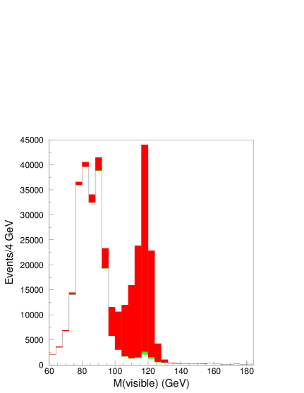
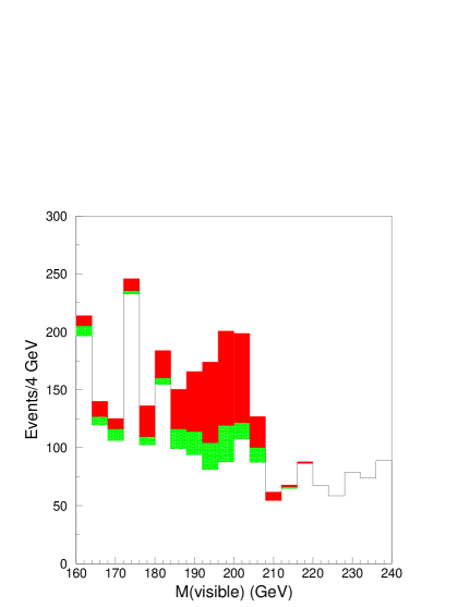
Figure 90: Histograms of $M({\rm visible})$ following $b\bar{b}$ selection cuts for background and signal assuming $M_{h}=120$ GeV (left) and $M_{h}=200$ GeV (right). The histograms contain non-Higgs SM background (white), $h\rightarrow b\bar{b}$ (red) and other Higgs decays (green).

3.2 $\bf h\rightarrow\gamma\gamma$

Decays of Higgs bosons to photon pairs are selected by requiring:

$$N({\rm chg})=0,\quad N({\rm imp})=0,$$

$$N({\rm jet})=2,\quad M_{h}-2\ {\rm GeV}<M({\rm visible})<M_{h}+1\ {\rm GeV}.$$ (80)

Histograms of $M({\rm visible})$ are shown in Fig. 91 assuming Higgs boson masses of 120 and 160 GeV. The SM background is almost entirely $\mbox{$e^{+}e^{-}$}\rightarrow\nu\nu\gamma\gamma$.

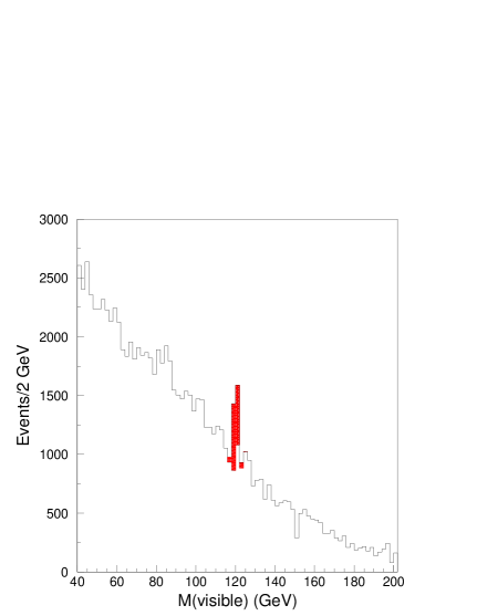
Figure 91: Histograms of $M({\rm visible})$ following $\gamma\gamma$ selection cuts for background and signal assuming $M_{h}=120$ GeV (left) and $M_{h}=160$ GeV (right). The histograms contain non-Higgs SM background (white) and $h\rightarrow\gamma\gamma$ (red).

3.3 $\bf h\rightarrow WW,\ \ gg$

Decays of Higgs bosons to $WW$ or $WW^{*}$ are selected by requiring:

$$16\leq N({\rm chg})\leq 44,\quad N({\rm imp})\leq 6,$$

$$4\leq N({\rm jet})\leq 5,\quad M_{h}-10\ {\rm GeV}<M({\rm visible})<M_{h}+6\ {\rm GeV}.$$ (81)

The histogram of $M({\rm visible})$ following the $WW$ cuts is shown in the left-hand side of Fig. 92 for a Higgs boson mass of 120 GeV. The non-Higgs SM background is mostly $\mbox{$e^{+}e^{-}$}\rightarrow e\nu W$. There is also a substantial Higgs boson background consisting of $h\rightarrow gg$ (63%), $h\rightarrow bb$ (14%), $h\rightarrow cc$ (12%) and $h\rightarrow ZZ^{*}$(12%). In order to isolate the $h\rightarrow WW$ signal from the other Higgs decay modes, events are forced into 4 jets and a neural net analysis is performed using the 4-momentum dot products between pairs of jets and the event variables $E({\rm visible})$, $p_{T}({\rm visible})$, $N({\rm chg})$, $N({\rm imp})$, and $N({\rm jet})$. The results of this neural net analysis are shown in the right-hand side of Fig. 92.

The background from $h\rightarrow b\bar{b},\ c\bar{c},\ ZZ^{*}$ is small enough that Higgs branching fraction results from $\sqrt{s}=350$ GeV can be used to account for these decays without introducing significant systematic errors. However, the contribution from $h\rightarrow gg$ can only be dealt with by measuring $\sigma\cdot B_{WW}$ and $\sigma\cdot B_{gg}$ simultaneously. To that end the decay $h\rightarrow gg$ is selected by requiring:

$$11\leq N({\rm chg})\leq 49,\quad N({\rm imp})\leq 6,$$

$$2\leq N({\rm jet})\leq 4,\quad M_{h}-10\ {\rm GeV}<M({\rm visible})<M_{h}+6\ {\rm GeV}.$$ (82)

An $h\rightarrow gg$ neural net analysis is performed with a set of variables identical to that used in the $h\rightarrow WW$ neural net analysis. The results of the simultaneous fit of $\sigma\cdot B_{WW}$ and $\sigma\cdot B_{gg}$ for $M_{h}=115,120,140,160$ GeV are shown in rows 2 and 3 of Table 31. For $M_{h}=200$ GeV the $h\rightarrow gg$ decay mode is negligible and so a simultaneous fit of $\sigma\cdot B_{WW}$ and $\sigma\cdot B_{ZZ}$ is made where the $ZZ$ selection cuts are the same as the $WW$ selection cuts and an $h\rightarrow ZZ$ neural net analysis is performed to separate $h\rightarrow ZZ$ from $h\rightarrow WW$.

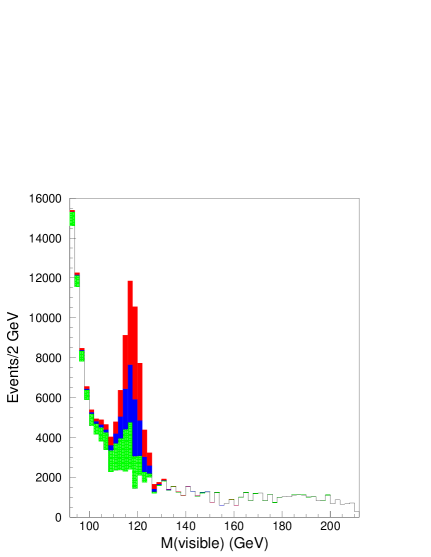
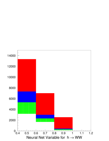
Figure 92: Histograms of $M({\rm visible})$ (left) and the $h\rightarrow WW$ neural net variable (right) following $WW$ selection cuts assuming $M_{h}=120$ GeV. The histograms contain non-Higgs SM background (white), $h\rightarrow W\bar{W}$ (red), $h\rightarrow gg$ (blue), and $h\rightarrow b\bar{b},\ c\bar{c},\ ZZ^{*}$ (green).

Table 31: Statistical accuracies for the measurement of $\sigma\cdot B_{xx}$ for different Higgs decay modes $h\rightarrow xx$ at $\sqrt{s}=1000$ GeV.

	Higgs Mass (GeV)
	115	120	140	160	200
$\Delta(\sigma\cdot B_{bb})/(\sigma\cdot B_{bb})$	$\pm 0.003$	$\pm 0.004$	$\pm 0.005$	$\pm 0.018$	$\pm 0.090$
$\Delta(\sigma\cdot B_{WW})/(\sigma\cdot B_{WW})$	$\pm 0.021$	$\pm 0.013$	$\pm 0.005$	$\pm 0.004$	$\pm 0.005$
$\Delta(\sigma\cdot B_{gg})/(\sigma\cdot B_{gg})$	$\pm 0.014$	$\pm 0.015$	$\pm 0.025$	$\pm 0.145$
$\Delta(\sigma\cdot B_{\gamma\gamma})/(\sigma\cdot B_{\gamma\gamma})$	$\pm 0.053$	$\pm 0.051$	$\pm 0.059$	$\pm 0.237$
$\Delta(\sigma\cdot B_{ZZ})/(\sigma\cdot B_{ZZ})$					$\pm 0.013$

4 Measurement of Higgs Branching Fractions and the total Higgs Decay Width

The measurements of $\sigma\cdot B_{xx}$ in Table 31 can be converted into model independent measurements of Higgs branching fractions and the total Higgs decay width if they are combined with measurements of the branching fractions $B_{bb}^{*}$ and $B_{WW}^{*}$ from $\sqrt{s}=350$ GeV:

$$B_{xx} = (\sigma\cdot B_{xx})(\sigma\cdot B_{WW})^{-1}B_{WW}^{*}=(\sigma\cdot B_{xx})(\sigma\cdot B_{bb})^{-1}B_{bb}^{*}$$

$$\Gamma_{tot} \propto (\sigma\cdot B_{bb})(B_{bb}^{*})^{-1}(B_{WW}^{*})^{-1}=(\sigma\cdot B_{bb})^{2}(\sigma\cdot B_{WW})^{-1}(B_{bb}^{*})^{-2}.$$ (83)

The assumed values for the errors on $B_{bb}^{*}$ and $B_{WW}^{*}$ are shown in Table 32. The errors are taken from the TESLA TDR[316] when the branching fractions are small. For large branching fractions, however, it is better to use the direct method[470] for measuring branching fractions because binomial statistics reduce the error by a factor of $\sqrt{1-B_{xx}}$.

Utilizing the relations in Eq.(6) a least squares fit is performed to obtain measurement errors for $B_{bb}$, $B_{WW}$, $B_{gg}$, $B_{\gamma\gamma}$, and $\Gamma_{tot}$ at a fixed value of $M_{h}$. The results are summarized in Table 33. Compared to branching fraction measurements at $\sqrt{s}=350$ GeV[316] the results of Table 33 provide a significant improvement for Higgs decay modes with small branching fractions, such as $B_{bb}$ for $160<M_{h}<200$ GeV, $B_{WW}$ for $115<M_{h}<140$ GeV and $B_{gg}$ and $B_{\gamma\gamma}$ for all Higgs masses.

Table 32: Assumed branching fraction errors for Higgs boson decays to $\ bb\$ and $WW$ from measuements made at $\sqrt{s}=350$ GeV with 500 fb^-1 luminosity.

	Higgs Mass (GeV)
	115	120	140	160	200
$\Delta B_{bb}^{*}/B_{bb}^{*}$	$\pm 0.015$	$\pm 0.017$	$\pm 0.026$	$\pm 0.065$	$\pm 0.340$
$\Delta B_{WW}^{*}/B_{WW}^{*}$	$\pm 0.061$	$\pm 0.051$	$\pm 0.025$	$\pm 0.010$	$\pm 0.025$

Table 33: Relative accuracies for the measurement of Higgs branching fractions and the Higgs boson total decay width obtained by combining results from Tables 31 and 32.

	Higgs Mass (GeV)
	115	120	140	160	200
$\Delta B_{bb}/B_{bb}$	$\pm 0.015$	$\pm 0.016$	$\pm 0.018$	$\pm 0.020$	$\pm 0.090$
$\Delta B_{WW}/B_{WW}$	$\pm 0.024$	$\pm 0.020$	$\pm 0.018$	$\pm 0.010$	$\pm 0.025$
$\Delta B_{gg}/B_{gg}$	$\pm 0.021$	$\pm 0.023$	$\pm 0.035$	$\pm 0.146$
$\Delta B_{\gamma\gamma}/B_{\gamma\gamma}$	$\pm 0.055$	$\pm 0.054$	$\pm 0.062$	$\pm 0.237$
$\Delta\Gamma_{tot}/\Gamma_{tot}$	$\pm 0.035$	$\pm 0.034$	$\pm 0.036$	$\pm 0.020$	$\pm 0.050$

5 Conclusion

The couplings of Higgs bosons in the mass range $115<M_{h}<200$ GeV can continue to be measured as the energy of an $e^{+}e^{-}$ linear collider is upgraded to $\sqrt{s}=1000$ GeV. The Higgs event rate is so large that some of the rarer decay modes that were inaccessible at $\sqrt{s}=350$ GeV can be probed at $\sqrt{s}=1000$ GeV, such as $h\rightarrow b\bar{b}$ for $M_{h}=200$ GeV, and $h\rightarrow gg,\ \gamma\gamma$ for $M_{h}=140$ GeV. The Higgs physics results from $\sqrt{s}=1000$ GeV will help provide a more complete picture of the Higgs boson profile.

Acknowledgements.

M. Krämer would like to thank the DESY Theory Group for their hospitality and financial support. This work has been supported in part by the European Union under contract HPRN-CT-2000-00149. M. L. Ciccolini is partially supported by ORS Award ORS/2001014035. R. Harlander is supported by DFG, contract HA 2990/2-1. This research was supported in part by the National Science Foundation under grant No. PHY-0139953. and by the Hungarian Scientific Research Fund grants OTKA T-038240, by the US Department of Energy, contract DE-FG0396ER40969, by the European Community’s Human Potential Programme under contract HPRN-CT-2002-00326, [V.D.], by the INTAS 00-0679, CERN-INTAS 99-377, YSF 02/239 and Universities of Russia UR.02.03.002 grants and by U.S. Department of Energy contract DE-AC03-76SF00515. During this work, C. Balazs was supported by the U.S. Department of Energy HEP Division under contracts DE-FG02-97ER41022 and W-31-109-ENG-38, and by LPNHE-Paris. N. Kidonakis’ research has been supported by a Marie Curie Fellowship of the European Community programme “Improving Human Research Potential” under contract number HPMF-CT-2001-01221. A. Sabio Vera acknowledges the support of PPARC (Postdoctoral Fellowship: PPA/P/S/1999/00446). E. Boos thanks the Humboldt Foundation for the Bessel Research Award. J.F. Gunion is supported by the U.S. Department of Energy and the Davis Institute for High Energy Physics. S. Moretti thanks the UK-PPARC and the Royal Society (London, U.K.) for financial support. C. Hugonie is supported by the European Commission RTN grant HPRN-CT-2000-00148. J.F. Gunion, C. Hugonie and U. Ellwanger thank the France-Berkeley fund for partial support of this research. A. Sopczak thanks the Particle Physics and Astronomy Research Council for financial support.

References

-
[1]
D. Rainwater, M. Spira and D. Zeppenfeld, Proceedings “Physics at TeV
Colliders”, Les Houches, France, 2001, hep-ph/0203187;
M. Spira, Proceedings “SUSY02”, Hamburg, Germany, 2002, hep-ph/0211145. - [2] F. Maltoni, Z. Sullivan and S. Willenbrock, Phys. Rev. D67 (2003) 093005.
-
[3]
E. Boos and T. Plehn, Phys. Rev. D69 (2004) 094005;
T. Plehn, Phys. Rev. D67 (2003) 014018. -
[4]
R.M. Barnett, H.E. Haber and D.E. Soper, Nucl. Phys. B306
(1988) 697;
F. I. Olness and W.-K. Tung, Nucl. Phys. B308 (1988) 813;
D. Dicus and S. Willenbrock, Phys. Rev. D39 (1989) 751. -
[5]
D. Dicus, T. Stelzer, Z. Sullivan and S. Willenbrock, Phys. Rev.
D59 (1999) 094016;
C. Balazs, H.–J. He and C.P. Yuan, Phys. Rev. D60 (1999) 114001. - [6] S. Dittmaier, M. Krämer and M. Spira, hep-ph/0309204.
- [7] S. Dawson, C. Jackson, L. Reina and D. Wackeroth, Phys. Rev. D69 (2004) 074027.
- [8] J. Pumplin et. al., JHEP 0207 (2002) 012; D. Stump et. al., JHEP 0310 (2003) 046.
- [9] J. Campbell, R. K. Ellis, F. Maltoni and S. Willenbrock, Phys. Rev. D67 (2003) 095002.
- [10] R. Harlander and W. Kilgore, Phys. Rev. D68 (2003) 013001.
- [11] S. Dittmaier, M. Krämer and M. Spira, paper in preparation.
- [12] S. Dawson, C. Jackson, L. Reina and D. Wackeroth, paper in preparation.
- [13] T. Affolder et al. [CDF Collaboration], Phys. Rev. Lett. 86 (2001) 4472.
-
[14]
ATLAS Collaboration, Technical Design Report, CERN–LHCC 99–14 (May 1999);
CMS Collaboration, Technical Proposal, CERN–LHCC 94–38 (December 1994);
S. Dawson, D. Dicus, C. Kao, and R. Malhotra, hep-ph/0402172. -
[15]
W. Beenakker, S. Dittmaier, M. Krämer, B. Plümper, M. Spira and
P.M. Zerwas, Phys. Rev. Lett. 87 (2001) 201805, Nucl. Phys.
B653 (2003) 151;
L. Reina and S. Dawson, Phys. Rev. Lett. 87 (2001) 201804;
L. Reina, S. Dawson and D. Wackeroth, Phys. Rev. D65 (2002) 053017;
S. Dawson, L.H. Orr, L. Reina and D. Wackeroth, Phys. Rev. D67 (2003) 071503;
S. Dawson, C. Jackson, L.H. Orr, L. Reina and D. Wackeroth, Phys. Rev. D68 (2003) 034022. - [16] M. Carena et al., Report of the Tevatron Higgs Working Group, hep-ph/0010338.
- [17] H. M. Georgi, S. L. Glashow, M. E. Machacek and D. V. Nanopoulos, Phys. Rev. Lett. 40 (1978) 692.
- [18] S. Dawson, Nucl. Phys. B 359 (1991) 283.
- [19] A. Djouadi, M. Spira and P. M. Zerwas, Phys. Lett. B 264 (1991) 440.
- [20] M. Spira, A. Djouadi, D. Graudenz and P. M. Zerwas, Nucl. Phys. B 453 (1995) 17.
- [21] M. Krämer, E. Laenen and M. Spira, Nucl. Phys. B 511 (1998) 523.
- [22] R. V. Harlander, Phys. Lett. B 492 (2000) 74.
- [23] S. Catani, D. de Florian and M. Grazzini, JHEP 0105 (2001) 025, JHEP 0201 (2002) 015.
- [24] R. V. Harlander and W. B. Kilgore, Phys. Rev. D 64 (2001) 013015,
- [25] R. V. Harlander and W. B. Kilgore, Phys. Rev. Lett. 88 (2002) 201801.
- [26] C. Anastasiou and K. Melnikov, Nucl. Phys. B 646 (2002) 220.
- [27] V. Ravindran, J. Smith and W. L. van Neerven, Nucl. Phys. B 665 (2003) 325.
- [28] S. Catani, D. de Florian, M. Grazzini and P. Nason, JHEP 0307 (2003) 028.
- [29] A. D. Martin, R. G. Roberts, W. J. Stirling and R. S. Thorne, Phys. Lett. B 531 (2002) 216.
- [30] S. Alekhin, Phys. Rev. D 68 (2003) 014002.
- [31] A. Djouadi and P. Gambino, Phys. Rev. Lett. 73 (1994) 2528; K. G. Chetyrkin, B. A. Kniehl and M. Steinhauser, Nucl. Phys. B 490 (1997) 19.
- [32] J. Pumplin, D. R. Stump, J. Huston, H. L. Lai, P. Nadolsky and W. K. Tung, JHEP 0207 (2002) 012.
- [33] A. Djouadi and S. Ferrag, preprint CERN-TH-2003-214 [hep-ph/0310209].
- [34] A. D. Martin, R. G. Roberts, W. J. Stirling and R. S. Thorne, Eur. Phys. J. C 28 (2003) 455.
- [35] A. D. Martin, R. G. Roberts, W. J. Stirling and R. S. Thorne, preprint IPPP-03-45 [hep-ph/0308087].
- [36] W. L. van Neerven and A. Vogt, Nucl. Phys. B 568 (2000) 263, Nucl. Phys. B 588 (2000) 345, Phys. Lett. B 490 (2000) 111.
- [37] S. A. Larin, P. Nogueira, T. van Ritbergen and J. A. Vermaseren, Nucl. Phys. B 492 (1997) 338; A. Retey and J. A. Vermaseren, Nucl. Phys. B 604 (2001) 281; S. Moch, J. A. M. Vermaseren and A. Vogt, Nucl. Phys. B 646 (2002) 181.
- [38] R. K. Ellis, I. Hinchliffe, M. Soldate and J. J. van der Bij, Nucl. Phys. B 297 (1988) 221; U. Baur and E. W. Glover, Nucl. Phys. B 339 (1990) 38.
- [39] D. de Florian, M. Grazzini and Z. Kunszt, Phys. Rev. Lett. 82 (1999) 5209.
- [40] V. Ravindran, J. Smith and W. L. Van Neerven, Nucl. Phys. B 634 (2002) 247.
- [41] C. J. Glosser and C. R. Schmidt, JHEP 0212 (2002) 016.
- [42] G. Parisi and R. Petronzio, Nucl. Phys. B 154 (1979) 427; Y. L. Dokshitzer, D. Diakonov and S. I. Troian, Phys. Rep. 58 (1980) 269; J. C. Collins, D. E. Soper and G. Sterman, Nucl. Phys. B 250 (1985) 199.
- [43] S. Catani et al., hep-ph/0005025, in the Proceedings of the CERN Workshop on Standard Model Physics (and more) at the LHC, eds. G. Altarelli and M.L. Mangano (CERN 2000-04, Geneva, 2000), p. 1.
- [44] S. Catani, E. D’Emilio and L. Trentadue, Phys. Lett. B 211 (1988) 335.
- [45] R. P. Kauffman, Phys. Rev. D 45 (1992) 1512.
- [46] D. de Florian and M. Grazzini, Phys. Rev. Lett. 85 (2000) 4678, Nucl. Phys. B 616 (2001) 247.
- [47] S. Catani, D. de Florian and M. Grazzini, Nucl. Phys. B 596 (2001) 299.
- [48] S. Catani, D. de Florian and M. Grazzini, JHEP 0105 (2001) 025; R. V. Harlander and W. B. Kilgore, Phys. Rev. D 64 (2001) 013015, Phys. Rev. Lett. 88 (2002) 201801; C. Anastasiou and K. Melnikov, Nucl. Phys. B 646 (2002) 220; V. Ravindran, J. Smith, W. L. van Neerven, Nucl. Phys. B 665 (2003) 325.
- [49] G. Bozzi, S. Catani, D. de Florian and M. Grazzini, Phys. Lett. B 564 (2003) 65.
- [50] C. Balazs and C. P. Yuan, Phys. Lett. B 478 (2000) 192; E. L. Berger and J. w. Qiu, Phys. Rev. D 67 (2003) 034026; A. Kulesza, G. Sterman, W. Vogelsang, preprint BNL-HET-03/20 [hep-ph/0309264].
- [51] A. D. Martin, R. G. Roberts, W. J. Stirling and R. S. Thorne, Eur. Phys. J. C 23 (2002) 73.
- [52] A. D. Martin, R. G. Roberts, W. J. Stirling and R. S. Thorne, Eur. Phys. J. C 28 (2003) 455.
- [53] C. T. H. Davies, B. R. Webber and W. J. Stirling, Nucl. Phys. B 256 (1985) 413.
- [54] G. A. Ladinsky and C. P. Yuan, Phys. Rev. D 50 (1994) 4239.
- [55] F. Landry, R. Brock, P. M. Nadolsky and C. P. Yuan, Phys. Rev. D 67 (2003) 073016.
- [56] A. Kulesza and W. J. Stirling, hep-ph/0307208.
- [57] Report of the Tevatron Higgs working group, M. Carena, J. S. Conway, H. E. Haber, J. D. Hobbs et al. [hep-ph/0010338].
- [58] A. Stange, W. J. Marciano and S. Willenbrock, Phys. Rev. D 49 (1994) 1354 [hep-ph/9309294] and Phys. Rev. D 50 (1994) 4491 [hep-ph/9404247].
- [59] ATLAS Collaboration, Technical Design Report, Vol. 2, CERN–LHCC–99–15.
- [60] G. L. Bayatian et al., CMS Technical Proposal, CERN-LHCC-94-38 (1994).
- [61] A. Djouadi et al., “The Higgs working group: Summary report”, proceedings of the Workshop On Physics At TeV Colliders, Les Houches, France, 1999 [hep-ph/0002258].
- [62] D. Cavalli et al., “The Higgs working group: Summary report”, proceedings of the Workshop On Physics At TeV Colliders, Les Houches, France, 2001 [hep-ph/0203056].
-
[63]
S. L. Glashow, D. V. Nanopoulos and A. Yildiz,
Phys. Rev. D 18 (1978) 1724;
Z. Kunszt, Z. Trócsány and W. J. Stirling, Phys. Lett. B 271 (1991) 247. - [64] T. Han and S. Willenbrock, Phys. Lett. B 273, 167 (1991); J. Ohnemus and W. J. Stirling, Phys. Rev. D 47 (1993) 2722; H. Baer, B. Bailey and J. F. Owens, Phys. Rev. D 47 (1993) 2730; S. Mrenna and C. P. Yuan, Phys. Lett. B 416 (1998) 200 [hep-ph/9703224]; M. Spira, Fortsch. Phys. 46 (1998) 203 [hep-ph/9705337]; A. Djouadi and M. Spira, Phys. Rev. D 62 (2000) 014004 [hep-ph/9912476].
- [65] D. A. Dicus and S. S. Willenbrock, Phys. Rev. D 34 (1986) 148; D. A. Dicus and C. Kao, Phys. Rev. D 38 (1988) 1008 [Erratum-ibid. D 42 (1990) 2412]; V. D. Barger, E. W. Glover, K. Hikasa, W. Y. Keung, M. G. Olsson, C. J. Suchyta and X. R. Tata, Phys. Rev. Lett. 57 (1986) 1672; B. A. Kniehl, Phys. Rev. D 42 (1990) 2253.
- [66] O. Brein, A. Djouadi and R. Harlander, Phys. Lett. B 579 (2004) 149 [hep-ph/0307206].
- [67] M. L. Ciccolini, S. Dittmaier and M. Krämer, Phys. Rev. D 68 (2003) 073003 [hep-ph/0306234].
- [68] R. Hamberg, W. L. van Neerven and T. Matsuura, Nucl. Phys. B 359 (1991) 343 [Erratum-ibid. B 644 (2002) 403]; W. L. van Neerven and E. B. Zijlstra, Nucl. Phys. B 382 (1992) 11.
- [69] V. D. Barger et al., Phys. Rev. Lett. 57 (1986) 1672; D. A. Dicus and C. Kao, Phys. Rev. D 38 (1988) 1008 [Erratum-ibid. D 42 (1990) 2412]; B. A. Kniehl, Phys. Rev. D 42 (1990) 2253.
- [70] A. D. Martin, R. G. Roberts, W. J. Stirling and R. S. Thorne, Phys. Lett. B 531 (2002) 216 [hep-ph/0201127].
- [71] J. Kripfganz and H. Perlt, Z. Phys. C 41 (1988) 319; H. Spiesberger, Phys. Rev. D 52 (1995) 4936 [hep-ph/9412286].
- [72] W. J. Stirling, talk given at the workshop Electroweak Radiative Corrections to Hadronic Observables at TeV Energies, Durham, UK, September 2003.
- [73] R. Kinnunen and D. Denegri, arXiv:hep-ph/9907291.
- [74] V. Drollinger, T. Muller and D. Denegri, arXiv:hep-ph/0111312.
- [75] E. Richter-Was and M. Sapinski. Acta Phys. Polon., B30:1001–1040, 1999.
- [76] B. P. Kersevan and E. Richter-Was. Eur. Phys. J., C25:379–389, 2002.
- [77] D. Zeppenfeld, R. Kinnunen, A. Nikitenko, and E. Richter-Was. Phys. Rev., D62:013009, 2000.
- [78] D. Zeppenfeld. eConf, C010630:P123, 2001.
- [79] A. Belyaev and L. Reina. JHEP, 08:041, 2002.
- [80] Tao Han, G. Valencia, and S. Willenbrock. Phys. Rev. Lett., 69:3274–3277, 1992.
- [81] W. Giele et al., arXiv:hep-ph/0204316.
- [82] H. Chehime and D. Zeppenfeld. Phys. Rev., D47:3898–3905, 1993.
- [83] D. Rainwater, R. Szalapski, and D. Zeppenfeld. Phys. Rev., D54:6680–6689, 1996.
- [84] V. A. Khoze, M. G. Ryskin, W. J. Stirling, and P. H. Williams. Eur. Phys. J., C26:429–440, 2003.
- [85] D. Rainwater, D. Zeppenfeld, and K. Hagiwara. Phys. Rev., D59:014037, 1999.
- [86] T. Plehn, D. Rainwater, and D. Zeppenfeld. Phys. Rev., D61:093005, 2000.
- [87] O. J. P. Eboli and D. Zeppenfeld. Phys. Lett., B495:147–154, 2000.
- [88] U. Baur and D. Zeppenfeld, arXiv:hep-ph/9309227.
- [89] T. Figy, C. Oleari, and D. Zeppenfeld. Phys. Rev., D68:073005, 2003.
- [90] C. Oleari and D. Zeppenfeld, arXiv:hep-ph/0310156.
- [91] J. Campbell and K. Ellis, MCFM - Monte Carlo for FeMtobarn processes, http://mcfm.fnal.gov/; E. L. Berger and J. Campbell, arXiv:hep-ph/0403194.
- [92] S. Catani, Y. L. Dokshitzer, and B. R. Webber. Phys. Lett., B285:291–299, 1992.
- [93] S. Catani, Y. L. Dokshitzer, M. H. Seymour, and B. R. Webber. Nucl. Phys., B406:187–224, 1993.
- [94] S.D. Ellis and D.E. Soper. Phys. Rev., D48:3160–3166, 1993.
- [95] G. C. Blazey et al., arXiv:hep-ex/0005012.
- [96] The CTEQ Collaboration, J. Pumplin, D.R. Stump, J. Huston, H.L. Lai, P. Nadolsky and W.K. Tung, JHEP 0207 (2002) 012, hep-ph/0201195.
- [97] The MRST Collaboration, A.D. Martin, R.G. Roberts, W.J. Stirling and R.S. Thorne, Eur. Phys. J. C28 (2003) 455, hep-ph/0211080.
- [98] S. Alekhin, Phys. Rev. D63 (2001) 094022 and Phys. Rev. D68 (2003) 014002.
- [99] A. Djouadi and S. Ferrag, hep-ph/0310209.
- [100] See the web site: http://mspira.home.cern.ch/mspira/proglist.html
- [101] T. Han and S. Willenbrock, Phys. Lett. B273 (1990) 167.
- [102] A. Djouadi and M. Spira, Phys. Rev. D62 (2000) 014004.
- [103] M. Spira, A. Djouadi, D. Graudenz and P. Zerwas, Nucl. Phys. B453 (1995) 17 and Phys. Lett. B318 (1993) 347; D. Graudenz, M. Spira, P. Zerwas, Phys. Rev. Lett. 70 (1993) 1372.
- [104] A. Djouadi, M. Spira and P.M. Zerwas, Phys. Lett. B264 (1991) 440; S. Dawson, Nucl. Phys. B359 (1991) 283.
- [105] W. Beenakker et al., Phys. Rev. Lett. 87 (2001) 201805 and Nucl. Phys. B653 (2003) 151; S. Dawson et al., Phys. Rev. Lett. 87 (2001) 201804 and Phys. Rev. D68 (2003) 034022.
- [106] R.V. Harlander and W. Kilgore, Phys. Rev. Lett. 88 (2002) 201801; C. Anastasiou and K. Melnikov, Nucl. Phys. B646 (2002) 220; V. Ravindran, J. Smith and W. L. van Neerven, hep-ph/0302135.
- [107] D. Abbaneo et al. hep-ex/0312023.
- [108] M. Dittmar and H. Dreiner. Phys. Rev., D55:167, 1997.
- [109] D. Rainwater and D. Zeppenfeld. Phys. Rev., D60:113004, 1999.
- [110] N. Kauer, T. Plehn, D. Rainwater, and D. Zeppenfeld. Phys. Lett., B503:113, 2001.
- [111] N. Akchurin et al. CMS-NOTE-2002/066; B. Mellado, ATL-CONF-2002-004; S. Asia et al., ATL-PHYS-2003-005; G. Azuelos and R. Mazini, ATL-PHYS-2003-004.
- [112] M. Dührssen. ATL-PHYS-2003-030 and references therein.
- [113] D. Rainwater. Phys. Lett., B503:320, 2001.
- [114] V. Drollinger, T. Müller, and D. Denegri. hep-ph/0201249 and hep-ph/0111312.
- [115] V. Kostioukhine et al. ATL-PHYS-2002-019; D. Green et al., FERMILAB-FN-705 (August 2001).
- [116] F. Maltoni, D. Rainwater, and S. Willenbrock. Phys. Rev., D66:034022, 2002.
- [117] J. A. Aguilar-Saavedra et al. hep-ph/0106315 and references therein; T. Abe et al. [American Linear Collider Working Group Collaboration], arXiv:hep-ex/0106056 and references therein.
- [118] D. Dicus, C. Kao, and S. Willenbrock. Phys. Lett., B203:457, 1988.
- [119] E. W. N. Glover and J. J. van der Bij. Nucl. Phys., B309:282, 1988.
- [120] F. Boudjema and E. Chopin. Z. Phys., C73:85, 1996.
- [121] V. A. Ilyin et al. Phys. Rev., D54:6717, 1996.
- [122] A. Djouadi, W. Kilian, M. Mühlleitner, and P. M. Zerwas. Eur. Phys. J., C10:27, 1999.
- [123] D. J. Miller and S. Moretti. Eur. Phys. J., C13:459, 2000.
- [124] M. Battaglia, E. Boos, and W. Yao. eConf, C010630:E3016, 2001.
- [125] C. Castanier, P. Gay, P. Lutz, and J. Orloff. hep-ex/0101028.
- [126] F. Gianotti et al. hep-ph/0204087.
- [127] U. Baur, T. Plehn, and D. Rainwater. Phys. Rev. Lett., 89:151801, 2002.
- [128] U. Baur, T. Plehn, and D. Rainwater. Phys. Rev., D67:033003, 2003.
- [129] A. Blondel, A. Clark and F. Mazzucato. ATL-PHYS-2002-029.
- [130] U. Baur, T. Plehn, and D. Rainwater. Phys. Rev., D68:033001, 2003.
- [131] U. Baur, T. Plehn and D. L. Rainwater, Phys. Rev. D 69 (2004) 053004 [arXiv:hep-ph/0310056].
- [132] T. Plehn, M. Spira, and P. M. Zerwas. Nucl. Phys., B479:46, 1996.
- [133] A. Djouadi, W. Kilian, M. Mühlleitner, and P. M. Zerwas. Eur. Phys. J., C10:45, 1999.
- [134] A. Dobrovolskaya and V. Novikov. Z. Phys., C52:427, 1991.
- [135] D. Dicus, K. Kallianpur, and S. Willenbrock. Phys. Lett., B200:187, 1988.
- [136] A. Abbasabadi, W. W. Repko, D. Dicus, and R. Vega. Phys. Lett., B213:386, 1988.
- [137] W. Y. Keung. Mod. Phys. Lett., A2:765, 1987.
- [138] V. Barger, T. Han, and R. J. N. Phillips. Phys. Rev., D38:2766, 1988.
- [139] S. Dawson, S. Dittmaier, and M. Spira. Phys. Rev., D58:115012, 1998.
- [140] D. Zeppenfeld. Phys. Rev., D61:077501, 2000.
- [141] K. Hagiwara et al. Phys. Rev., D66:010001, 2002.
- [142] M. El Kacimi and R. Lafaye. ATL-PHYS-2002-015.
- [143] M. Battaglia and A. de Roeck. these proceedings.
- [144] S. Zhu. Phys. Rev., D67:075006, 2003.
- [145] T. Plehn. Phys. Rev., D67:014018, 2003.
- [146] N. Kidonakis and J. F. Owens. Phys. Rev., D61:094004, 2000.
- [147] N. Kidonakis and J. F. Owens. Int. J. Mod. Phys. A 19 (2004) 149.
- [148] N. Kidonakis and J. F. Owens. Phys. Rev., D63:054019, 2001.
- [149] N. Kidonakis. Phys. Rev., D64:014009, 2001.
- [150] N. Kidonakis and R. Vogt. Phys. Rev., D68:114014, 2003.
- [151] N. Kidonakis and A. Belyaev. JHEP, 12:004, 2003.
- [152] N. Kidonakis and A. Sabio Vera. JHEP, 02:027, 2004.
- [153] N. Kidonakis and G. Sterman. Phys. Lett., B387:867, 1996.
- [154] N. Kidonakis and G. Sterman. Nucl. Phys., B505:321, 1997.
- [155] N. Kidonakis. Int. J. Mod. Phys., A15:1245, 2000.
- [156] N. Kidonakis. Int. J. Mod. Phys., A19:1793, 2004.
- [157] A. Pilaftsis, Phys. Rev. D 58 (1998) 096010; Phys. Lett. B 435 (1998) 88.
-
[158]
T. Hahn, S. Heinemeyer, W. Hollik, G. Weiglein,
in preparation; see also:
S. Heinemeyer, W. Hollik, G. Weiglein, Comp. Phys. Comm. 124 2000 76; hep-ph/0002213.
The codes are accessible from www.feynhiggs.de. -
[159]
S. Heinemeyer,
Eur. Phys. Jour. C 22 (2001) 521;
M. Frank, S. Heinemeyer, W. Hollik, G. Weiglein, hep-ph/0212037. - [160] M. Frank, S. Heinemeyer, W. Hollik, G. Weiglein, hep-ph/0202166.
- [161] G. Degrassi, S. Heinemeyer, W. Hollik, P. Slavich, G. Weiglein, Eur. Phys. Jour. C 28 (2003) 133.
- [162] S. Heinemeyer, W. Hollik, G. Weiglein, Eur. Phys. Jour. C 16 (2000) 139.
- [163] A. Djouadi et al., Phys. Rev. Lett. 78 (1997) 3626; Phys. Rev. D 57 (1998) 4179; S. Heinemeyer, G. Weiglein, JHEP 0210 (2002) 072; hep-ph/0301062.
- [164] S. Heinemeyer, D. Stöckinger, G. Weiglein, hep-ph/0312264, to appear in Nucl. Phys. B, hep-ph/0405255.
- [165] A. Djouadi, J. Kalinowski, M. Spira, Comput. Phys. Commun. 108 (1998) 56.
- [166] J. Lee, A. Pilaftsis et al., hep-ph/0307377.
- [167] P. Skands et al., hep-ph/0311123.
- [168] B. Allanach et al., Eur. Phys. Jour. C 25 (2002) 113.
- [169] M. Carena, S. Heinemeyer, C. Wagner and G. Weiglein, Eur. Phys. Jour. C 26 (2003) 601.
- [170] T. Hahn, M. Pérez-Victoria, Comput. Phys. Commun. 118 (1999) 153.
- [171] The LEP Electroweak Working Group and the SLD Heavy Flavour Group, CERN-EP/2002-091, hep-ex/0212036; see also lepewwg.web.cern.ch.
- [172] J. R. Forshaw, D. A. Ross and B. E. White, JHEP 0110 (2001) 007.
- [173] J. R. Forshaw, A. Sabio Vera and B. E. White, JHEP 0306 (2003) 059.
- [174] D. Bardin et al, Comput. Phys. Commun. 133 (2001) 229.
- [175] S. R. Coleman and E. Weinberg, Phys. Rev. D 7 (1973) 1888.
- [176] R. Jackiw, Phys. Rev. D 9 (1974) 1686.
- [177] J. Iliopoulos, C. Itzykson and A. Martin, Rev. Mod. Phys. 47 (1975) 165.
- [178] B. Kastening, Phys. Lett. B 283 (1992) 287.
- [179] C. Ford, D. R. Jones, P. W. Stephenson and M. B. Einhorn, Nucl. Phys. B 395 (1993) 17.
- [180] M. Quiros, Helv. Phys. Acta 67 (1994) 451.
- [181] H.-J. He, Y.-P. Kuang, C.-P. Yuan, and B. Zhang, Phys. Lett. B554(2003)64; B. Zhang, Y.-P. Kuang, H.-J. He, and C.-P. Yuan, Phys. Rev. D67(2003)114024.
- [182] R. Sekhar Chivukula and V. Koulovassilopoulos, Phys. Lett. B309(1993)371.
- [183] K. Hagiwara, S. Ishihara, R. Szalapski, and D. Zeppenfeld, Phys. Rev. D48 (1993) 2182; W. Buchmüller and D. Wyler, Nucl. Phys. B268 (1986) 621; C. J. C. Burgess and H. J. Schnitzer, Nucl. Phys. B228 (1983) 454; C. N. Leung, S. T. Love and S. Rao, Z. Phys. 31 (1986) 433; A. De Rújula, M. B. Gavela, P. Hernández and E. Massó, Nucl. Phys. B384 (1992) 3.
- [184] For a review, M. C. Gonzales-Garcia, Int. J. Mod. Phys. A 14 (1999) 3121.
- [185] M.S. Chanowitz, Phys. Lett. B322 (1994) 147; Phys. Lett. B347 (1995) 387.
- [186] J. Bagger et al., Phys. Rev. D49 (1994) 1246.
- [187] J. Bagger et al., Phys. Rev. D52 (1995) 3878.
- [188] D. Zeppenfeld, hep-ph/0203123, Snowmass contribution; T. Plehn, D. Rainwater, and D. Zeppenfeld, Phys. Rev. Lett. 88 (2002) 051801.
- [189] K. Hagiwara, S. Ishihara, J. Kamoshita, and B.A. Kniehl, Eur. Phys. J. 14 (2000) 457.
- [190] K. Hagiwara et al. [Particle Data Group Collaboration], Phys. Rev. D 66 (2002) 010001.
- [191] K. Monig, arXiv:hep-ph/0308133.
- [192] P. Aurenche et al. 1990. in Proc. Large Hadron Collider Workshop, Aachen, edited by G. Jarlskod and D. Rein, CERN 90-10/ECFA 90-133.
- [193] L. Fayard and G. Unal. Search for higgs decays using photons with eagle. Atlas Internal Note ATL-PHYS-92-001 and Addenda 1&2, (1992).
- [194] G. Eynard, Study of associated higgs boson production with the ATLAS detector at LHC, (in French), CERN-THESIS-2000-036.
- [195] T. Binoth, J. P. Guillet, E. Pilon, and M. Werlen. Eur. Phys. J., C16:311–330, 2000.
- [196] C. Balazs, E. L. Berger, S. Mrenna, and C. P. Yuan. Phys. Rev., D57:6934–6947, 1998.
- [197] C. Balazs and C. P. Yuan. Phys. Rev., D59:114007, 1999.
- [198] C. Balazs, P. Nadolsky, C. Schmidt, and C. P. Yuan. Phys. Lett., B489:157–162, 2000.
- [199] C. Balazs, arXiv:hep-ph/9906422.
- [200] C. Balazs and C. P. Yuan, Phys. Lett., B478:192–198, 2000.
- [201] C. Balazs, J. Huston, and I. Puljak. Phys. Rev., D63:014021, 2001.
- [202] C. Balazs, arXiv:hep-ph/0008160.
- [203] Torbjorn Sjostrand et al., Comput. Phys. Commun., 135:238–259, 2001.
- [204] C. Balazs and C. P. Yuan, Phys. Rev., D56:5558–5583, 1997.
- [205] M. Spira, arXiv:hep-ph/9510347.
- [206] V. Ravindran, J. Smith, and W. L. van Neerven, Mod. Phys. Lett., A18:1721–1734, 2003.
- [207] Zvi Bern, Lance Dixon, and Carl Schmidt, Phys. Rev., D66:074018, 2002.
- [208] S. Kretzer, H. L. Lai, F. I. Olness and W. K. Tung, arXiv:hep-ph/0307022.
- [209] D. R. Stump, A new generation of CTEQ parton distribution functions with uncertainty analysis, Prepared for 31st International Conference on High Energy Physics (ICHEP 2002), Amsterdam, The Netherlands, 24-31 Jul 2002.
- [210] M. Wielers, talk at the 4th ATLAS workshop, Athens, 21-25 May 2003.
- [211] E. Richter-Was, D. Froidevaux, and L. Poggioli, ATLfast 2.0 a fast simulation package for ATLAS, ATLAS Internal Note ATL-PHYS-98-131 (1998).
- [212] J. Smith, private communication.
- [213] M. Wielers, Photon identification with the ATLAS detector, ATL-PHYS-99-016.
- [214] C. Schmidt, private communication.
- [215] John Campbell and R. K. Ellis, Phys. Rev., D65:113007, 2002.
- [216] J. Campbell, R. K. Ellis and D. L. Rainwater, Phys. Rev. D 68 (2003) 094021 [arXiv:hep-ph/0308195].
- [217] Tilman Plehn, David Rainwater, and Dieter Zeppenfeld, Phys. Lett., B454:297–303, 1999.
- [218] Tilman Plehn, David Rainwater, and Dieter Zeppenfeld. Phys. Rev. Lett., 88:051801, 2002.
- [219] G. Azuelos et al., Search for the SM Higgs boson using vector boson fusion at the LHC, Prepared for Workshop on Physics at TeV Colliders, Les Houches, France, 21 May - 1 Jun 2001.
- [220] N. Akchurin et al., Study of low mass higgs using at CMS, CMS-NOTE-2001/016.
- [221] E. Richter-Was, Prospects for the observability of the WH and ZH, H–¿bb channel in 14 TeV pp and 2 TeV ppbar collisions (etmiss + bb final state), ATL-PHYS-2000-023.
- [222] V. Drollinger, T. Müller and D. Denegri, Prospects for higgs boson searches in the channel , CMS-NOTE-2002/006.
- [223] M. N. Dubinin, V. A. Ilyin, and V. I. Savrin. hep-ph/9712335.
- [224] S. Abdullin et al. Phys. Lett., B431:410–419, 1998.
- [225] R. K. Ellis, I. Hinchliffe, M. Soldate, and J. J. van der Bij. Nucl. Phys., B297:221, 1988.
- [226] E. E. Boos, M. N. Dubinin, V. A. Ilyin, A. E. Pukhov, and V. I. Savrin. hep-ph/9503280.
- [227] T. Sjostrand, L. Lonnblad, and S. Mrenna. hep-ph/0108264.
- [228] V. Zmushko. ATL-PHYS-2002-020.
- [229] J.M. Campbell and R.K. Ellis. Phys. Rev., D62:114012, 2000. http://mcfm.fnal.gov/mcfm-3.4.uu.
- [230] V. Del Duca, F. Maltoni, Z. Nagy, and Z. Trócsányi. JHEP, 04:059, 2003.
- [231] V. Del Duca, W. Kilgore, C. Oleari, C. Schmidt, and D. Zeppenfeld. Nucl. Phys., B616:367–399, 2001.
- [232] M.A. Shifman, A. I. Vainshtein, M. B. Voloshin, and V.I. Zakharov. Sov. J. Nucl. Phys., 30:711–716, 1979.
- [233] J.R. Ellis, M.K. Gaillard, and D. V. Nanopoulos. Nucl. Phys., B106:292, 1976.
- [234] U. Baur and E. W. N. Glover. Nucl. Phys., B339:38–66, 1990.
- [235] V. Del Duca, W. Kilgore, C. Oleari, C. R. Schmidt, and D. Zeppenfeld. Phys. Rev., D67:073003, 2003.
- [236] V. Del Duca, W.B. Kilgore, and F. Maltoni. Nucl. Phys., B574:851–873, 2000.
- [237] Z. Bern, L.J. Dixon, and D.A. Kosower. Nucl. Phys., B437:259–304, 1995.
- [238] A. Signer. Phys. Lett., B357:204–210, 1995.
- [239] D. de Florian and Z. Kunszt. Phys. Lett., B460:184–188, 1999.
- [240] S. Frixione. Phys. Lett., B429:369–374, 1998.
- [241] S. Catani and B. R. Webber. JHEP, 10:005, 1997.
- [242] S. Asai et al., Search for the Standard Model Higgs Boson in ATLAS using Vector Boson Fusion, ATLAS Scientific Note SN-ATLAS-2003-024 (2003), submitted to EPJ, hep-ph/0402254.
- [243] R. Barate et al., Phys. Lett., B565:61–75, 2003.
- [244] Martin G. Grunewald, Electroweak precision data: Global Higgs analysis, 2003, hep-ex/0304023.
- [245] N. Kauer and D. Zeppenfeld, Phys. Rev., D65:014021, 2002.
- [246] N. Kauer, Phys. Rev., D67:054013, 2003.
- [247] N. Kauer, hep-ph/0404045
- [248] E. Richter-Was and M. Sapinski, Search for the SM and MSSM Higgs Boson in the , Channel, Acta Phys.Polon.B30:1001-1040,1999 ; V. Drollinger, T. Muller and D. Denegri, Searching for Higgs Bosons in Association with Top Quark Pairs in the Decay Mode, CMS NOTE 2001/054, hep-ph/0111312.
- [249] A. Pukhov et al., CompHEP - a Package for Evaluation of Feynman Diagrams and Integration over multi Particle Phase Space, INP-MSU 98-41/542.
- [250] M. Mangano et al., ALPGEN, a Generator for hard Multiparton Processes in hadronic Collisions, CERN-TH-2002-129, FTN-T-2002-06
- [251] A. De Roeck, V.A. Khoze, A.D. Martin, R. Orava and M.G. Ryskin, Eur. Phys. J. C25 (2002) 391.
- [252] M. Carena and H. Haber, Prog. Part. Nucl. Phys. 50 (2003) 63 and references therein.
- [253] A.B. Kaidalov, V.A. Khoze, A.D. Martin and M.G. Ryskin, Eur. Phys. J., C31:387–396, 2003.
- [254] A.B. Kaidalov, V.A. Khoze, A.D Martin and M.G. Ryskin, hep-ph/0311023.
- [255] V.A. Khoze, A.D. Martin and M.G. Ryskin, Eur. Phys. J. C23 (2002) 311.
- [256] V.A. Khoze, A.D. Martin and M.G. Ryskin, Eur. Phys. J. C19 (2001) 477, erratum C20 (2001) 599.
- [257] M. Boonekamp, R. Peschanski and C. Royon, Phys. Rev. Lett. 87 (2001) 251806.
- [258] M. Boonekamp, R. Peschanski, A. De Roeck and C. Royon, Phys. Lett. B550 (2002) 93.
- [259] V.A. Khoze, A.D Martin and M.G. Ryskin, Eur. Phys. J. C26 (2002) 229.
- [260] B.E. Cox, J.R. Forshaw and B. Heinemann, Phys. Lett. B540 (2002) 263.
- [261] S.Erhan, V.T.Kim and P.E.Schlein, hep-ph/0312342.
- [262] D. Graudenz and G. Veneziano Phys. Lett. B365 302 (1996), hep-ph/9508401.
- [263] A. Bialas and P.V. Landshoff, Phys. Lett. B256 (1991) 540.
- [264] J.-R. Cudell and O.F. Hernandez, Nucl. Phys. B471 (1996) 471.
- [265] E.M. Levin, hep-ph/9912402 and references therein.
- [266] V.A. Khoze, A.D. Martin and M.G. Ryskin, Eur. Phys. J. C14 (2000) 525 and references therein.
- [267] B.E. Cox, J.R. Forshaw, J.S. Lee, J. Monk and A. Pilaftsis, Phys. Rev. D68 (2003)
- [268] C. Royon, hep-ph/0308283 and references therein.
- [269] V.A. Khoze, A.D Martin and M.G. Ryskin, hep-ph/0401078.
- [270] V.P. Nomokonov for the Helsinki Group in Forward Physics and Luminosity Determination at LHC, Helsinki, Finland, 31 October to 4 November 2000, World Scientific (2001) 164, ed. R. Orava, K. Huitu, V. Khoze and S. Tapprogge.
- [271] R. Orava, Diffraction at LHC, Workshop on Diffractive Physics, LISHEP 2002, Rio de Janeiro, Brasil, 4–8 February 2002, acceptance and resolution figures refer to the simulation studies by J. Lamsa (Iowa Sate University, Ames, Ill.) and R. Orava.
- [272] R. Enberg, G. Ingelman, A. Kissavos and N. Timneanu, Phys. Rev. Lett. 89 (2002) 081801.
- [273] CDF Collaboration: T. Affolder et al., Phys. Rev. Lett. 85 (2000) 4215.
- [274] K. Goulianos (for the CDF collaboration), FERMILAB-CONF-03-277-E, Aug 2003, hep-ph/0308183; A. Wyatt(for the CDF collaboration), FERMILAB-Conf-03/324-E, 2003.
- [275] CDF Collaboration: T. Affolder et al., Phys. Rev. Lett. 84 (2000) 5043.
- [276] V.A. Khoze, A.D. Martin and M.G. Ryskin, Eur. Phys. J. C18 (2000) 167 and references therein.
- [277] T. Sjöstrand, Comput. Phys. Commun. 82 (1994) 74.
- [278] K. Osterberg, talk at the workshop on physics with forward proton taggers at the Tevatron and LHC, http://glodwick.hep.man.ac.uk/conference/
- [279] V.A. Petrov and R.A. Ryutin, hep-ph/0311024
- [280] M. Boonekamp, R. Peschanski, C. Royon, Nucl. Phys. B669 (2003) 277, Erratum-ibid. B676 (2004) 493, hep-ph/0301244.
- [281] M. Heyssler, Z.Kunszt and W.J.Stirling, Phys. Lett. B406 (1997) 95.
- [282] S.Erhan and P.E.Schlein, private communication.
- [283] E. Boos, L. Dudko and T. Ohl, Eur. Phys. J. C 11, 473 (1999); E.E. Boos and L.V. Dudko, “Singularities of Feynman Diagrams and Optimal Kinematic Variables for Neural Networks”, DØ Note 3612, February 1999.
- [284] L. Dudko, In Proceedings of AIHENP’99, Crete, April, 1999; V. M. Abazov et al. [D0 Collaboration], Phys. Lett. B 517, 282 (2001).
- [285] A. Pukhov et al., hep-ph/9908288; E.E. Boos et al., INP MSU 94-36/358 and SNUTP-94-116, hep-ph/9503280.
-
[286]
http://www-d0.fnal.gov/~dudko/mcdb/ - [287] P.C. Bhat, R. Gilmartin, H.B. Prosper, Phys.Rev. D62 (2000) 074022; hep-ph/0006162.
-
[288]
http://www.physics.rutgers.edu/~jconway/soft/shw/shw.html - [289] Gregory Mahlon, McGill/98-34, hep-ph/9811281
- [290] G. Mahlon and S. Parke, Phys. Rev. D55 (1997) 7249; G. Mahlon and S. Parke, Phys. Lett. B476, (2000) 323; E.E. Boos, A.V. Sherstnev Phys. Lett. B534, (2002) 97.
- [291] ALEPH, DELPHI, L3 and OPAL, The LEP Higgs Working Group, hep-ex/0107031.
- [292] F. Borzumati, J.-L. Kneur and N. Polonsky. Phys. Rev., D60:115011, 1999.
- [293] D.J. Miller, S. Moretti, D.P. Roy and W.J. Stirling. Phys. Rev., D61:055011, 2000.
- [294] G. Corcella et al. JHEP, 01:010, 2001.
- [295] G. Corcella et al., Herwig 6.5 release note, hep-ph/0210213.
- [296] S. Moretti, K. Odagiri, P. Richardson, M.H. Seymour and B.R. Webber, JHEP, 04:028, 2002.
- [297] M. Guchait and S. Moretti, JHEP, 01:001, 2002.
- [298] S. Raychaudhuri and D.P. Roy, Phys. Rev., D52:1556, 1995.
- [299] Pablo Garcia-Abia and Wolfgang Lohmann, Eur. Phys. J. direct, C2:2, 2000.
- [300] K. Cranmer, B. Mellado, W. Quayle and S. L. Wu, arXiv:hep-ph/0307242.
- [301] I. Puljak, Potentiel de decouverte du boson de Higgs dans le canal avec le detecteur CMS, Dissertation, Ecole Polytechnique, Palaiseau, France (2000).
- [302] CMS: The electromagnetic calorimeter. Technical design report, CERN-LHCC-97-33.
- [303] K. Cranmer, B. Mellado, W. Quayle and Sau Lan Wu, Search for Higgs Boson Decay Using Vector Boson Fusion, ATLAS Note ATL-PHYS-2003-036 (2003), hep-ph/0401088
- [304] M. Dubinin, Higgs boson signal in the reaction two forward jets, CMS-NOTE-2001/022.
- [305] M. N. Dubinin, V. A. Ilyin, and V. I. Savrin, Light Higgs boson signal at LHC in the reaction lepton, Prepared for 12th International Workshop on High-Energy Physics and Quantum Field Theory (QFTHEP 97), Samara, Russia, 4-10 Sep 1997.
- [306] D. Green et al. J. Phys., G26:1751–1764, 2000.
- [307] J. Leveque, J. B. de Vivie, V. Kostioukhine, and A. Rozanov, Search for the Standard Model Higgs boson in the channel, ATL-PHYS-2002-019.
- [308] V. Cavasinni and D. Costanzo. Search for using like-sign leptons, ATL-PHYS-2000-013.
- [309] J. Cammin and M. Schumacher, The ATLAS discovery potential for the channel , ATL-PHYS-2003-024.
- [310] V. Drollinger, T. Muller, and D. Denegri, Searching for Higgs bosons in association with top quark pairs in the decay mode, CMS-NOTE-2001/054.
- [311] Dan Green, Kaori Maeshima, Richard Vidal, Weimin Wu, and Shuichi Kunori, A study of t anti-t + higgs at CMS. FERMILAB-FN-0705.
- [312] M. Schumacher, talk given at the “Advanced Studies Institute, Physics at LHC”, Prague, July 2003, see: asipraha.web.cern.ch/asipraha/2003/LHC/.
- [313] Lawrence J. Hall, Riccardo Rattazzi, and Uri Sarid, Phys. Rev., D50:7048–7065, 1994.
- [314] S. Heinemeyer, W. Hollik, and G. Weiglein, Phys. Lett., B455:179–191, 1999.
- [315] S. Heinemeyer, W. Hollik, and G. Weiglein. FeynHiggsFast: A program for a fast calculation of masses and mixing angles in the Higgs sector of the MSSM, hep-ph/0002213.
- [316] J. A. Aguilar-Saavedra et al., ECFA/DESY LC Physics Working Group, TESLA Technical Design Report Part III: Physics at an Linear Collider, hep-ph/0106315.
- [317] LEP Higgs Working Group for Higgs boson searches Proceedings International Europhysics Conference on High Energy Physics (HEP 2001), Budapest, Hungary, 12-18 Jul 2001 [hep-ex/0107029 and hep-ex/0107030].
- [318] H. Baer, C. Chen, M. Drees, F. Paige, and X. Tata Phys. Rev. D59 (1999) 055014.
- [319] D. Denegri, W. Majerotto, and L. Rurua Phys. Rev. D60 (1999) 035008.
- [320] J. Gunion, L. Poggioli, R. V. Kooten, C. Kao, and P. Rowson hep-ph/9703330.
- [321] L. J. Hall, R. Rattazzi and U. Sarid Phys. Rev. D50 (1994) 7048; M. Carena, M. Olechowski, S. Pokorski and C. E. Wagner Nucl. Phys. B426 (1994) 269; M. Carena, D. Garcia, U. Nierste and C. E. Wagner Nucl. Phys. B577 (2000) 88; J. Guasch, P. Häfliger and M. Spira hep-ph/0305101.
- [322] L. Bellucci, Dissertation, Universita degli studi di Firenze (2001).
- [323] S. Lehti, Prospects for the Detection of the MSSM Higgs Bosons Decaying into Tau Leptons in the CMS Detector, Dissertation, University of Helsinki, Report Series in Physics, HU-P-D93 (2001); S. Lehti, Study of gg, H CMS NOTE 2002/035.
- [324] R. Kinnunen and A. Nikitenko, CMS NOTE 1997/106.
- [325] R. Kinnunen and A. Nikitenko, CMS NOTE 2003/006.
- [326] R. Kinnunen, CMS NOTE 2000/045.
- [327] S. Dittmaier, M. Spira, and M. Krämer, hep-ph/0309204.
- [328] T. Plehn, Phys. Rev. D67 (2003) 014018 [hep-ph/0206121]; E. Boos and T. Plehn, Higgs-Boson Production Induced by Bottom Quarks, hep-ph/0304034.
- [329] J. Campbell, R. K. Ellis, F. Maltoni, and S. Willenbrock, hep-ph/0204093.
- [330] S. Dawson, C. Jackson, L. Reina, and D. Wackeroth, hep-ph/0311067.
- [331] S. Dittmaier, M. Krämer, and M. Spira, private communication.
- [332] M. Spira http://people.web.psi.ch/spira/proglist.html.
- [333] CMS Collaboration, CERN/LHCC 2002-26, CMS TDR 6.2.
- [334] P. Salmi, R. Kinnunen, and N. Stepanov, CMS NOTE 2002/024.
- [335] S. Lehti, CMS NOTE 2001/019.
- [336] J. Gunion, S. Kraml, and F. Moortgat, private communication.
- [337] S. L. Glashow, Nucl. Phys. B22 (1961) 579
- [338] S. Weinberg, Phys. Rev. Lett. 19 (1967) 1264
- [339] A. Salam, Proceedings to the Eigth Nobel Symposium, May 1968, ed: N. Svartholm (Wiley, 1968) 357
- [340] S.L. Glashow, J. Iliopoulos and L. Maiani, Phys. Rev. D2 (1970) 1285
- [341] P.W. Higgs, Phys. Lett. 12 (1964) 132
- [342] P.W. Higgs, Phys. Rev. Lett. 13 (1964) 508
- [343] P.W. Higgs, Phys. Rev. 145 (1966) 1156
- [344] F. Englert, R. Brout, Phys. Rev. Lett. 13 (1964) 321
- [345] G.S. Guralnik, C.R. Hagen and T.W.B. Kibble, Phys. Rev. Lett. 13 (1964) 585
- [346] T.W.B. Kibble, Phys. Rev. 155 (1967) 1554
- [347] ATLAS Collaboration, Detector and Physics Performance Technical Design Report, CERN-LHCC/99-14 (1999)
- [348] H.M. Georgi, S.L. Glashow, M.E. Machacek and D.V. Nanopoulos, Phys. Rev. Lett. 40 (1978) 11
- [349] R. Cahn and S. Dawson, Phys. Lett. B136 (1984) 196
- [350] G. Kane, W. Repko and W. Rolnick, Phys. Lett. B148 (1984) 367
- [351] D.L. Rainwater and D. Zeppenfeld, Phys. Rev. D60 (1999) 113004
- [352] N. Kauer, T. Plehn, D.L. Rainwater and D. Zeppenfeld, Phys. Lett. B503 (2001) 113
- [353] T. Plehn, D.L. Rainwater and D. Zeppenfeld, Phys. Rev. D61 (2000) 093005
- [354] D.L. Rainwater and D. Zeppenfeld, JHEP 9712 (1997) 005
- [355] T. Sjöstrand, Comp. Phys. Comm. 82 (1994) 74
- [356] T. Sjöstrand et al., Comp. Phys. Comm. 135 (2000) 238
- [357] M. Spira, VV2H Programe, home.cern.ch/m/mspira/www.proglist.html
- [358] H.L. Lai et al., Eur. Phys. J. C12 (2000) 375
- [359] E. Richter-Was, D. Froidevaux and L. Poggioli, ATLFAST2.0 a Fast Simulation Package for ATLAS, ATLAS Note ATL-PHYS-98-131 (1998)
- [360] C. Buttar, K. Jakobs and R. Harper, Weak boson fusion as a search mode for an intermediate mass SM Higgs boson at ATLAS, ATL-PHYS-2002-033 (2002)
- [361] S. Frixione and B.R. Webber, JHEP 0206 (2002) 029
- [362] S. Frixione and B.R. Webber, JHEP 0308 (2003) 007
- [363] G. Corcella et al., JHEP 0101 (2001) 010
- [364] G. Corcella et al., HERWIG 6.5: an Event Generator for Hadron Emission Reactions with Interfering Gluons, hep-ph/0011363
- [365] T. Stelzer and W.F. Long, Phys. Comm. 81 (1994) 357
- [366] F. Maltoni and T. Stelzer, MadEvent: Automatic Event Generation with MadGraph, hep-ph/0208156 (2002)
-
[367]
Wisconsin Higgs Project,
Sotfware web page,
http://www-wisconsin.cern.ch/physics/software.html - [368] Y.Q. Fang, B. Mellado, W. Quayle, S. Paganis and Sau Lan Wu, A Study of the background at LHC, ATLAS internal Communication ATL-COM-PHYS-2003-043 (2003)
- [369] D. Zeppenfeld, private communication
- [370] R. Mazini, private communication
- [371] D. Zeppenfeld et al., http://pheno.physics.wisc.edu/Software/MadCUP/
- [372] M. Wall, GAlib: A C++ Library of Genetic Algorithm Components, http://lancet.mit.edu/ga/
- [373] K. Cranmer, B. Mellado, W. Quayle and Sau Lan Wu, Confidence Level Calculations in the Search for Higgs Bosons Decay Using Vector Boson Fusion, ATLAS Note ATL-PHYS-2003-008 (2003)
- [374] K. Cranmer, B. Mellado, W. Quayle and Sau Lan Wu, Challenges of Moving the LEP Higgs Statistics to the LHC, physics/0312050 (2003)
- [375] R.D. Cousins and V.L. Highland, Nucl. Instrum. Methods A320 (1992) 331
- [376] K. Cranmer, B. Mellado, W. Quayle and Sau Lan Wu, Neural Network Based Search for Higgs Boson Produced via VBF with for , ATLAS Note ATL-PHYS-2003-007 (2003)
- [377] F. James and M. Roos, Comp. Phys. Comm. 10 (1975) 343
- [378] D.L. Rainwater, Intermediate-Mass Higgs Searches in Weak Boson Fusion, Ph.D. thesis, University of Wisconsin - Madison, 1999 [hep-ph/9908378].
- [379] M.L. Mangano et al., ALPGEN, a Generator for Hard Multiparton Processes in Hadronic Collisions, hep-ph/0206293 (2002)
- [380] CDF Collaboration, F. Abe et al., Phys. Rev. Lett. 77 (1996) 448
- [381] CDF Collaboration, F. Abe et al., Phys. Rev. Lett. 79 (1997) 4760
- [382] K. Cranmer, B. Mellado, W. Quayle and Sau Lan Wu, Search for Higgs Boson Decay with Using Vector Boson Fusion, ATLAS internal Communication ATL-COM-PHYS-2003-035 (2003)
- [383] K. Cranmer, B. Mellado, W. Quayle and Sau Lan Wu, Neural Network Based Search for Higgs Boson Produced via VBF with , ATLAS Note, in preparation
- [384] G. Martinez, E. Gross, G. Mikenberg and L. Zivkovic, Prospects for Light Higgs Observation in the Channel at the LHC, ATLAS Note ATL-PHYS-2003-001 (2003)
- [385] K. Cranmer, B. Mellado, W. Quayle and Sau Lan Wu, Application of K Factors in the Analysis at the LHC, ATLAS Note ATL-PHYS-2003-025 (2003), hep-ph/0307242
- [386] H. Baer, M. Bisset, D. Dicus, C. Kao and X. Tata, Phys. Rev. D 47 (1993) 1062.
- [387] H. Baer, M. Bisset, C. Kao and X. Tata, Phys. Rev. D 50 (1994) 316 [arXiv:hep-ph/9402265].
- [388] F. Moortgat, S. Abdullin and D. Denegri, arXiv:hep-ph/0112046.
- [389] M. A. Bisset, UMI-95-32579
- [390] M. Bisset, M. Guchait and S. Moretti, Eur. Phys. J. C 19 (2001) 143 [arXiv:hep-ph/0010253].
- [391] M. Bisset, F. Moortgat and S. Moretti, Eur. Phys. J. C 30 (2003) 419 [arXiv:hep-ph/0303093].
- [392] S. Moretti, Pramana 60 (2003) 369 [arXiv:hep-ph/0205104].
- [393] K. A. Assamagan et al., Prepared for Workshop on Physics at TeV Colliders, Les Houches, France, 21 May - 1 Jun 2001
- [394] LEP SUSY Working Group web page, http://www.cern.ch/LEPSUSY/.
- [395] G. Corcella et al., arXiv:hep-ph/0201201.
- [396] H. Baer, F. E. Paige, S. D. Protopopescu and X. Tata, arXiv:hep-ph/0001086.
- [397] http://www.hep.phy.cam.ac.uk/richardn/HERWIG/ISAWIG/.
- [398] D. Denegri et al., arXiv:hep-ph/0112045.
- [399] M. Dzelalija, Z. Antunovic, D. Denegri and R. Kinnunen, Study of associated production Modes Wh, in the MSSM in CMS”, CMS-TN 96-091.
- [400] M. Spira, V2HV, http://people.web.psi.ch/spira/v2hv/
- [401] M.Dubinin et. Al, Light Higgs Boson Signal at LHC in the Reactions pp Gamma+Gamma+Jet and pp Gamma+Gamma+Lepton, CMS NOTE 1997/101
- [402] S. Abdullin, CMSJET, http://cmsdoc.cern.ch/ abdullin/cmsjet.html
- [403] CMS Collaboration, The Trigger and Data Acquisition project, Technical Design Report.
- [404] E. Boos, A. Djouadi, M. Mühlleitner and A. Vologdin, Phys. Rev., D66:055004, 2002.
- [405] E. Boos, A. Djouadi and A. Nikitenko, Phys. Lett., B578:384, 2004.
- [406] A. Pukhov et al., arXiv:hep-ph/9908288.
- [407] A. S. Belyaev et al., arXiv:hep-ph/0101232.
- [408] J. Campbell, R. K. Ellis, F. Maltoni, and S. Willenbrock, Phys. Rev., D67:095002, 2003.
- [409] E. Boos et al., in progress.
- [410] J. F. Gunion, Phys. Lett. B322, 125 (1994), [hep-ph/9312201].
- [411] V. Barger, R. J. N. Phillips and D. P. Roy, Phys. Lett. B324, 236 (1994), [hep-ph/9311372].
- [412] M. Carena, D. Garcia, U. Nierste and C. Wagner, Nucl. Phys. B577, 88 (2000), [hep-ph/9912516].
- [413] J. Guasch, P. Häfliger and M. Spira, Phys. Rev. D68, 115001 (2003), [hep-ph/0305101].
- [414] J. Guasch, W. Hollik and S. Peñaranda, Phys. Lett. B515, 367 (2001), [hep-ph/0106027].
- [415] J. Guasch, R. A. Jiménez and J. Solà, Phys. Lett. B360, 47 (1995), [hep-ph/9507461]; J. A. Coarasa, D. Garcia, J. Guasch, R. A. Jiménez and J. Solà, Eur. Phys. J. C2, 373 (1998), [hep-ph/9607485]; Phys. Lett. B425, 329 (1998), [hep-ph/9711472].
- [416] J. Guasch and J. Solà, Phys. Lett. B416, 353 (1998), [hep-ph/9707535].
- [417] A. Belyaev, D. Garcia, J. Guasch and J. Solà, Phys. Rev. D65, 031701 (2002), [hep-ph/0105053].
- [418] A. Belyaev, D. Garcia, J. Guasch and J. Solà, JHEP 06, 059 (2002), [hep-ph/0203031].
- [419] A. Belyaev, J. Guasch and J. Solà, Nucl. Phys. Proc. Suppl. 116, 296 (2003), [hep-ph/0210253].
- [420] M. Carena, H. E. Haber, H. E. Logan and S. Mrenna, Phys. Rev. D65, 055005 (2002), [hep-ph/0106116], [Erratum-ibid. D 65 (2002) 099902]; A. M. Curiel, M. J. Herrero, D. Temes and J. F. De Troconiz, Phys. Rev. D65, 075006 (2002), [hep-ph/0106267]; M. J. Herrero, S. Peñaranda and D. Temes, Phys. Rev. D64, 115003 (2001), [hep-ph/0105097]; H. E. Haber et al., Phys. Rev. D63, 055004 (2001), [hep-ph/0007006].
- [421] S. R. Slabospitsky and L. Sonnenschein, Comput. Phys. Commun. 148, 87 (2002), [hep-ph/0201292].
- [422] E. Richter-Was, D. Froidevaux and L. Poggioli, ATLFAST 2.0 a fast simulation package for ATLAS, ATL-PHYS-98-131.
- [423] K. A. Assamagan, Y. Coadou and A. Deandrea, Eur. Phys. J. direct C4, 9 (2002), [hep-ph/0203121].
- [424] K. A. Assamagan and Y. Coadou, Acta Phys. Polon. B33, 1347 (2002).
- [425] H. L. Lai et al. (CTEQ Collaboration), Eur. Phys. J. C12, 375 (2000), [hep-ph/9903282].
- [426] S. Jadach, J. H. Kühn and Z. Was, Comput. Phys. Commun. 64, 275 (1990).
- [427] M. Jezabek, Z. Was, S. Jadach and J. H. Kühn, Comput. Phys. Commun. 70, 69(1992).
- [428] S. Jadach, Z. Was, R. Decker and J. H. Kühn, Comput. Phys. Commun. 76, 361 (1993).
- [429] D. P. Roy, Phys. Lett. B459, 607 (1999), [hep-ph/9905542].
- [430] S. Moretti and D. P. Roy, Phys. Lett. B470, 209 (1999), [hep-ph/9909435].
- [431] B. C. Allanach et al., Eur. Phys. J. C25, 113 (2002), [hep-ph/0202233], [eConf C010630 (2001) P125].
- [432] T. Sjostrand, L. Lonnblad, S. Mrenna and P. Skands, arXiv:hep-ph/0308153.
- [433] J. Alwall, C. Biscarat, S. Moretti, J. Rathsman and A. Sopczak, arXiv:hep-ph/0312301.
- [434] J. L. Diaz-Cruz and O. A. Sampayo, Phys. Rev. D 50 (1994) 6820.
- [435] S. Raychaudhuri and D. P. Roy, Phys. Rev. D 52 (1995) 1556 [arXiv:hep-ph/9503251].
- [436] S. Raychaudhuri and D. P. Roy, Phys. Rev. D 53 (1996) 4902 [arXiv:hep-ph/9507388].
- [437] S. Moretti and W. J. Stirling, Phys. Lett. B 347 (1995) 291 [arXiv:hep-ph/9412209], Erratum-ibid. B 366 (1996) 451 [arXiv:hep-ph/9511351].
- [438] See http://durpdg.dur.ac.uk/hepdata/pdf.html.
- [439] J. F. Gunion, H. E. Haber, Gordon L. Kane, and S. Dawson. The Higgs Hunters’ Guide. Addison-Wesley, Reading, MA, 1990.
- [440] P. Salmi, R. Kinnunen, and N. Stepanov. Prospects of Detecting Massive Charged Higgs from Hadronic Decay in CMS. CMS NOTE 2002/024, 2002.
- [441] K. A. Assamagan. The Charged Higgs in Hadronic Decays with the ATLAS Detector. ATLAS-PHYS-99-017, 1999.
- [442] K. A. Assamagan and Y. Coadou. Prospects for the Determination of the Charged Higgs Mass and with ATLAS. ATLAS-PHYS-2001-017, 2001.
- [443] T. Plehn. Private communication.
- [444] L. Sonnenschein. Top mass determination in the semileptonic decay channel. CMS NOTE 2001/001, 2001.
- [445] F. Maltoni and T. Stelzer. JHEP, 02:027, 2003.
- [446] G. Altarelli and M.L. Mangano (eds.). Standard Model Physics (and more) at the LHC. Proceedings, Workshop, Geneva, Switzerland, May 25-26, October 14-15, 1999. Geneva, Switzerland: CERN (2000) 529 p.
- [447] S. Abdullin. CMSJET. CMS TN/94-180 (version of 10/10/2001), 2001.
- [448] V. Karimaki, V. Drollinger, A. Khanov, and N. Stepanov. Upgrade of Fast Tracker Response Simulation, the FATSIM utility. CMS IN-2000/034, 2000.
- [449] Technical Design Report: The TriDAS Project, Volume II: Data Acquisition & High Level Trigger. CERN/LHCC/2002-26, 2002.
- [450] R. Kinnunen. Study for Heavy Charged Higgs in with in CMS. CMS NOTE 2000/045, 2000.
- [451] T. Affolder et al. Phys. Rev., D64:032002, 2001.
- [452] J. Ellis, J. F. Gunion, H. Haber, L. Roszkowski, and F. Zwirner, Phys. Rev., D39:844, 1989.
- [453] U. Ellwanger, J. F. Gunion and C. Hugonie, arXiv:hep-ph/0111179.
- [454] J. F. Gunion, H. E. Haber and T. Moroi, arXiv:hep-ph/9610337.
- [455] B. A. Dobrescu, G. Landsberg, and K. T. Matchev, Phys. Rev., D63:075003, 2001.
- [456] C. Mariotti, for the LEP Higgs Working Group, Search of the standard model Higgs at LEP, Prepared for 31st International Conference on High Energy Physics (ICHEP 2002), Amsterdam, The Netherlands, 24-31 Jul 2002; see also LHWG Note/2002-01 at http://lephiggs.web.cern.ch/LEPHIGGS/papers/index.html; LEP Higgs Working Group, Searches for the Neutral Higgs Bosons of the MSSM: Preliminary Combined Results Using LEP Data Collected at Energies up to 209 GeV, LHWG Note 2001-04.
- [457] CMS Collaboration, Expected observability of SM Higgs in CMS with , CMS NOTE 1997/057.
- [458] U. Ellwanger and C. Hugonie, Eur. Phys. J., C25:297, 2002.
- [459] S. Moretti, private program.
- [460] U. Ellwanger, J. F. Gunion, C. Hugonie and S. Moretti, arXiv:hep-ph/0305109.
- [461] J. F. Gunion, H. E. Haber and R. Van Kooten, arXiv:hep-ph/0301023.
- [462] U. Ellwanger, J. Gunion, C. Hugonie, and S. Moretti, in progress.
- [463] M. Battaglia and A. De Roeck, eConf, C010630:E3066, 2001, hep-ph/0111307.
- [464] M. Battaglia and A. De Roeck, 2002, hep-ph/0211207.
- [465] International linear collider technical review committee, second report, 2003. SLAC-R-606.
- [466] W. Kilian, Whizard: Complete simulations for electroweak multi- particle processes, Prepared for 31st International Conference on High Energy Physics (ICHEP 2002), Amsterdam, The Netherlands, 24-31 Jul 2002.
- [467] Thorsten Ohl, Comput. Phys. Commun., 101:269, 1997, hep-ph/9607454.
- [468] M. Pohl and H. J. Schreiber, hep-ex/0206009.
- [469] T. Behnke, S. Bertolucci, R. D. Heuer and R. Settles, TESLA: The superconducting electron positron linear collider with an integrated X-ray laser laboratory. Technical design report. Pt. 4: A detector for TESLA, DESY-01-011
- [470] Jean-Claude Brient, The direct method to measure the higgs branching ratios at the future linear collider, LC-PHSM-2002-003.