Fragmentation Production of Triply Heavy Baryons at the LHC

Abstract

The triply heavy baryons in the standard model formed in direct $c$ and $b$ quark fragmentation are the $\Omega_{ccc}$, $\Omega_{ccb}$, $\Omega_{cbb}$ and $\Omega_{bbb}$ baryons. We calculate their fragmentation functions in leading order of perturbative QCD. The universal fragmentation probabilities fall within the range of $10^{-5}-10^{-7}$.We also evaluate their cross section at the LHC ($\sqrt{s}=14$ TeV) using next-to-leading order matrix elements for heavy quark-antiquark pair production. We present the differential cross sections as functions of the transverse momentum as well as the total cross sections. They range from a few nb to a few pb.

I Introduction

Heavy hadrons have been the focus of attention due to their interesting properties. The study of production and decay of such particles is interesting in two aspects. In the first place the question is whether QCD is the right theory to predict the properties of such objects through confirmation of the standard model predictions with experimental data. Secondly this research investigates the basic properties of the weak interactions at the fundamental level. These states have in general a large number of decay modes so that their observation and measurement of their properties require a large number of them to be produced. Their cross section at $e^{+}e^{-}$ collisions is very small therefore their identification needs a messier environment of the hadronic collider.

In the framework of the quark model, heavy baryons fall into three categories. States containing one heavy flavor such as $\Lambda_{c}$ and $\Lambda_{b}$, are interesting states due to the fact that they carry the original heavy flavor polarization [1]. Their production has been studied in interesting models [2]. They are also being studied experimentally [3]. The second category involves baryons with two heavy flavor like the states $\Xi_{cc}$, $\Xi_{bb}$ and $\Xi_{bc}$ [4]. They are treated within the approximate quark-diquark model [5]. The model treats the production of the so called diquark perturbatively similar to $B_{c}$ states [6]. Then, it can be proved that the formation of a baryon out of a diquark is almost the same as the fragmentation of an antiquark into a meson [7]. In this way one obtains the fragmentation functions, the total production probabilities and their event rates in a desired collider. Indeed the light degree of freedom within these states does not allow full perturbative calculation.

In the third category, we have baryons with three heavy constituents. Since the top quark cannot take part in strong interactions [8], there remains only the charm and bottom quarks to form such baryons.There have been attempts to evaluate the production of $\Omega_{ccc}$ and $\Omega_{bbb}$ in $e^{+}e^{-}$ and hadron colliders in the quark-diquark model [9] and also using perturbative QCD [10]. The results from $e^{+}e^{-}$ annihilation are very small indeed [11]. However sizable rates are expected in energetic hadron colliders [12]. Therefore the standard model production rates of these bound states can be compared with experimental data [13].

Consistent with the quark model of hadrons, the spectroscopy and production mechanism of heavy meson and baryon states have been treated satisfactorily. Specially the hadrons which contain $c$ and $b$ quarks or anti-quarks, are accounted for in the heavy quark limit where the hadronic bound state is understood and the perturbation theory is applied for the process of their production. This has been successful in the treatment of $B_{c}$ states both in theory [6], and in experiment [14] and also in the production of heavy diquarks in the treatment of doubly heavy baryons [4]. In this work we shall apply this procedure to the case of triply heavy baryons to obtain their fragmentation properties and cross section at the LHC. Many of these states may be observed at existing hadron colliders, specially at the Tevatron, however some others have very low event rates. Therefore we have chosen the LHC for the sake of integrity. Therefore in this work we consider a framework which treats all triply heavy baryons and obtain their fragmentation functions and estimate their production at the LHC.

Our plan is as follows. In section II we provide a general discussion of the fragmentation process of S-wave triply heavy baryons and calculation of their fragmentation functions. In sections III and IV we calculate the fragmentation functions for $c\rightarrow\Omega_{ccb}$ and $b\rightarrow\Omega_{ccb}$ which we have chosen to be the basic ones such that the other functions could be obtained from them by appropriate choices of quark masses and other baryon characteristic parameters. The inclusive production of these states at the LHC is studied in section V. Finally we discuss our results in section VI.

II Fragmentation of Triply heavy baryons

The fragmentation functions are process independent and can be applied to the $e^{+}e^{-}$, partonic and hadronic production processes. At sufficiently large transverse momenta, the dominant production mechanism is actually the fragmentation, the production of a parton with high transverse momentum which subsequently splits into a triply heavy state and other partons. Fig.1 shows the fragmentation of a heavy quark $Q$ into a triply heavy baryon $B(QQ^{\prime}Q^{\prime\prime})$ in lowest order perturbation theory. We will calculate such Feynman diagrams.

Figure 1: The lowest order Feynman diagrams contributing to the fragmentation of a heavy quark ($Q$) into a triply heavy baryon (B). The four momenta are labelled.

The fragmentation of a parton into a baryon state is described by fragmentation function $D(z,\mu)$, where $z$ is the longitudinal momentum fraction of the baryon state and $\mu$ is a fragmentation scale. The fragmentation function for the production of an S-wave triply heavy baryon $B$ in the fragmentation of a quark $Q$ is obtained from [15]

$$D_{Q}^{B}(z,\mu_{\circ}) = \frac{1}{2}\sum_{s}\int|T_{B}|^{2}$$ (1)

$$\times\delta^{3}(\overline{{\bf p}}+{\bf s^{\prime}}+{\bf t^{\prime}}-{\bf p}){\rm d^{3}\overline{{p}}}{\rm d^{3}{s^{\prime}}}{\rm d^{3}{t^{\prime}}},$$

where four momenta are as labelled in Fig 1. $T_{B}$ is the amplitude of the baryon production which involves the hard scattering amplitude $T_{H}$ and the non-perturbative smearing of the bound state. The average over initial and the sum over final spin states are assumed.

To absorb the soft behavior of the bound state into the hard scattering amplitude we have used the scheme introduced in [16]. The probability amplitude at large momentum transfer factorizes into a convolution of the hard-scattering amplitude $T_{H}$ and baryon distribution amplitude $\phi_{B}$, i.e.

$$T_{B}(p,\overline{p},s^{\prime},t^{\prime})=\int\bigl{[}dx\bigr{]}T_{H}(p,\overline{p},s^{\prime},t^{\prime},x_{i})\phi_{B}(x_{i},w^{2}).$$ (2)

where $\phi_{B}$ is the probability amplitude to find quarks co-linear up to a scale of $w^{2}$ in the baryonic bound state. In (2), $\bigl{[}dx\bigr{]}=dx_{1}dx_{2}dx_{3}\delta(1-x_{1}-x_{2}-x_{3})$ and $x_{i}$’s are the momentum fractions carried by the constituent quarks and finally $T_{H}$ is written in the following form in the old fashioned perturbation theory to keep the initial heavy quark on mass shell,

$$T_{H}=\frac{16\pi^{2}\alpha_{s}(2m_{Q^{\prime}})\alpha_{s}(2m_{Q^{\prime\prime}})MC_{F}}{2\sqrt{2p_{\circ}\overline{p}_{\circ}s^{\prime}_{\circ}t^{\prime}_{\circ}}}\frac{\Gamma}{(\overline{p}_{\circ}+s^{\prime}_{\circ}+t^{\prime}_{\circ}-p_{\circ})}.$$ (3)

Here $\Gamma$ represents an appropriate combination of the propagators and the spinorial parts of the amplitude. $\alpha_{s}=g^{2}/4\pi$ is the strong interaction coupling constant. $C_{F}$ is the color factor and $M=mm_{Q}m_{Q^{\prime}}m_{Q^{\prime\prime}}$ with $m$ being the baryon mass. Since we ignore the virtual motion of the baryon constituents, we propose a delta function type function to represent the probability amplitude of the baryon state

$$\phi_{B}=f_{B}\;\delta\biggl{\{}x_{i}-\frac{m_{i}}{m}\biggr{\}},$$ (4)

where $f_{B}$ is the baryon decay constant and is introduced similar to meson decay constant $f_{M}$. Putting this expression and (3) in (2) and carrying out the necessary integrations, we find

$$T_{B} = \frac{16\pi^{2}\alpha_{s}(2m_{Q^{\prime}})\alpha_{s}(2m_{Q^{\prime\prime}})MC_{F}f_{B}}{2\sqrt{2p_{\circ}\overline{p}_{\circ}s^{\prime}_{\circ}t^{\prime}_{\circ}}}$$ (5)

$$\times\frac{\Gamma}{(\overline{p}_{\circ}+s^{\prime}_{\circ}+t^{\prime}_{\circ}-p_{\circ})}.$$

With this amplitude we find the fragmentation function as

$$D_{Q}^{B}(z,\mu)=32\bigl{[}\pi^{2}\alpha_{s}({2m_{Q^{\prime}}})\alpha_{s}({2m_{Q^{\prime\prime}}})MC_{F}f_{B}\bigr{]}^{2}\int\frac{\frac{1}{2}\sum\overline{\Gamma}\Gamma\delta^{3}(\overline{\bf p}+{\bf s^{\prime}}+{\bf t^{\prime}}-{\bf p})}{p_{\circ}\overline{p}_{\circ}s^{\prime}_{\circ}t^{\prime}_{\circ}(\overline{p}_{\circ}+s^{\prime}_{\circ}+t^{\prime}_{\circ}-p_{\circ})^{2}}{\rm d^{3}}\overline{p}{\rm d^{3}}{s^{\prime}}{\rm d^{3}}{t^{\prime}}.$$ (6)

To proceed we need to specify our kinematics.

We let the baryon move in the $z$ direction after production, neglecting the virtual motion of the constituents. The initial state heavy quark has a transverse momentum which should be carried by the two antiquarks away through the final state jet. We have assumed that there will be only one jet in the final state. This assumption is justified due to the fact that the very high momentum of the initial heavy quark will predominantly be carried in the forward direction. Due to momentum conservation, the total transverse momentum of the two jets will be identical to the transverse momentum of the initial heavy quark. Therefore the antiquark’s contributions to this jet are assumed to be proportional to their masses.

The fragmentation parameter $z$, is defined as usual, i.e.

$$z=\frac{(E+p_{\|})_{B}}{(E+p_{\|})_{Q}},$$ (7)

which reduces to the following in the infinite momentum frame which we have adopted for our study

$$z=\frac{E_{B}}{E_{Q}}.$$ (8)

Now we set up our kinematics. According to Fig. 1 the baryon takes a fraction $z$ of the initial heavy quark’s energy (each constituent a fraction of $x_{1}$, $x_{2}$ and $x_{3}$) and the two anti-quarks take the remaining $1-z$ ($x_{4}$ and $x_{5}$ each). Thus the four momenta of the particles are parameterized as

$$\overline{p}_{\circ} = zp_{\circ}\;\;\;s_{\circ}=x_{1}zp_{\circ}\;\;\;r_{\circ}=x_{2}zp_{\circ}\;\;\;t_{\circ}=x_{3}zp_{\circ}$$

$$s^{\prime}_{\circ} = x_{4}(1-z)p_{\circ}\;\;\;t^{\prime}_{\circ}=x_{5}(1-z)p_{\circ}\;\;\;,$$ (9)

where the condition $x_{1}+x_{2}+x_{3}=1$ holds. Moreover regarding our assumptions we have

$${\bf s^{\prime}}_{T}=x_{4}{\bf p}_{T}\;\;\;\ {\bf t^{\prime}}_{T}=x_{5}{\bf p}_{T},$$ (10)

along with the constraint of $x_{4}+x_{5}=1$.

Fig. 2 shows the lowest order Feynman diagrams for the fragmentation of $\Omega_{ccc}$ and $\Omega_{bbb}$ (a,b), $\Omega_{ccb}$ in the $c$ quark fragmentation (c,d) and $\Omega_{ccb}$ in the $b$ quark fragmentation (e,f). There are similar diagrams contributing to $\Omega_{cbb}$ fragmentation in $b$ and $c$ quark fragmentation which are simply obtained by interchanging the $c$ and $b$ quarks in (c,d) and (e,f) respectively. Let us first consider the case of $c\rightarrow\Omega_{ccb}$.

Figure 2: The lowest order Feynman diagrams which contribute to different $\Omega$ baryon production. While (a) and (b) shows $c$ and $b$ quark fragmentation into $\Omega_{ccc}$ and $\Omega_{bbb}$ respectively, (c) and (d)contribute to $\Omega_{ccb}$ production in $c$ and (e) and (f) in $b$ quark fragmentation to the same state. Interchange of $c\longleftrightarrow b$ in last two pairs give the contributing diagrams to $\Omega_{cbb}$ in $b$ and $\Omega_{cbb}$ in $c$ quark fragmentation respectively.

III $\Omega_{ccb}$ in $c$ quark fragmentation

Here the diagrams (c) and (d) in Fig 2 are relevant. In each diagram there are three propagators. In this specific case for the diagram (c) we find the combination

$$G = \frac{1}{8m_{1}^{2}m_{2}^{3}m^{\prime}f^{3}(z)},$$ (11)

where one third of the power of $f$ comes from each propagator, $m^{\prime}=(m_{1}+m_{2})$ and that

$$f(z)=1+\frac{m}{2m^{\prime}}\frac{1-z}{z}+\frac{m^{\prime}}{2m}\Bigl{(}1+\frac{p_{T}^{2}}{m^{\prime 2}}\Bigr{)}\frac{z}{(1-z)}.$$ (12)

In the case of diagram (d) we have

$$G^{\prime}=\frac{1}{16m_{1}^{4}m_{2}^{2}f^{3}(z)}.$$ (13)

We put the dot products of the relevant four vectors in the following form

$$s^{\prime}.r=m_{1}^{2}\alpha\;\;\;r.p=m_{1}^{2}\beta\;\;\;s^{\prime}.p=m_{1}^{2}\gamma$$ (14)

where

$$\alpha=\frac{1}{2}\biggl{[}\frac{m}{m^{\prime}}\frac{1-z}{z}+\frac{m^{\prime}}{m}\Bigl{(}1+\frac{p_{T}^{2}}{m^{\prime 2}}\Bigr{)}\frac{z}{1-z}\biggr{]},$$ (15)

$$\beta=\frac{1}{2}\biggl{[}\frac{m_{1}}{m}\Bigl{(}1+\frac{p_{T}^{2}}{m_{1}^{2}}\Bigr{)}z+\frac{m}{m_{1}}\frac{1}{z}\biggr{]},$$ (16)

$$\gamma = \frac{1}{2}\biggl{[}\frac{m_{1}}{m^{\prime}}\Bigl{(}1+\frac{p_{T}^{2}}{m_{1}^{2}}\Bigr{)}(1-z)$$ (17)

$$+\frac{m^{\prime}}{m_{1}}\Bigl{(}1+\frac{p_{T}^{2}}{m^{\prime 2}}\Bigr{)}\frac{1}{1-z}-\frac{2p_{T}^{2}}{m_{1}m^{\prime}}\biggr{]}.$$

In obtaining the above results we have used (9) and (10) with $x_{1}=x_{2}=m_{1}/m\,;x_{3}=m_{2}/m,\;x_{4}=m_{1}/m^{\prime}$ and $x_{5}=m_{2}/m^{\prime}$.

In this case the $\Gamma$ in (6) reads

$$\Gamma=\;G\overline{u}(t)\gamma^{\rho}v(t^{\prime})\Bigl{[}\overline{u}(r)\gamma_{\rho}(\hbox to0.0pt{/\hss}q+m_{1})\gamma_{\nu}u(p)\Bigr{]}\overline{u}(s)\gamma^{\nu}v(s^{\prime})+G^{\prime}\overline{u}(s)\gamma^{\nu}v(s^{\prime})\Bigl{[}\overline{u}(r)\gamma_{\nu}(\hbox to0.0pt{/\hss}q^{\prime}+m_{1})\gamma_{\rho}u(p)\Bigr{]}\overline{u}(t)\gamma^{\rho}v(t^{\prime}).$$ (18)

From which we find

$$\overline{\Gamma}\Gamma = \;\;G^{2}\Bigl{[}(\hbox to0.0pt{/\hss}s^{\prime}-m_{1})\gamma^{\mu}(\hbox to0.0pt{/\hss}s+m_{1})\gamma^{\nu}\Bigr{]}T_{\mu\sigma\rho\nu}\Bigl{[}(\hbox to0.0pt{/\hss}t^{\prime}-m_{2})\gamma^{\sigma}(\hbox to0.0pt{/\hss}t+m_{2})\gamma^{\rho}\Bigr{]}+$$ (19)

$$\;G^{\prime 2}\Bigl{[}(\hbox to0.0pt{/\hss}t^{\prime}-m_{2})\gamma^{\sigma}(\hbox to0.0pt{/\hss}t+m_{2})\gamma^{\rho}\Bigr{]}T_{\sigma\mu\nu\rho}\Bigl{[}(\hbox to0.0pt{/\hss}s^{\prime}-m_{1})\gamma^{\mu}(\hbox to0.0pt{/\hss}s+m_{1})\gamma^{\nu}\Bigr{]}+$$

$$GG^{\prime}\Bigl{[}(\hbox to0.0pt{/\hss}s^{\prime}-m_{1})\gamma^{\mu}(\hbox to0.0pt{/\hss}s+m_{1})\gamma^{\nu}\Bigr{]}T_{\mu\sigma\nu\rho}\Bigl{[}(\hbox to0.0pt{/\hss}t^{\prime}-m_{2})\gamma^{\sigma}(\hbox to0.0pt{/\hss}t+m_{2})\gamma^{\rho}\Bigr{]}+$$

$$GG^{\prime}\Bigl{[}(\hbox to0.0pt{/\hss}t^{\prime}-m_{2})\gamma^{\sigma}(\hbox to0.0pt{/\hss}t+m_{2})\gamma^{\rho}\Bigr{]}T_{\sigma\mu\rho\nu}\Bigl{[}(\hbox to0.0pt{/\hss}s^{\prime}-m_{1})\gamma^{\mu}(\hbox to0.0pt{/\hss}s+m_{1})\gamma^{\nu}\Bigr{]},$$

where

$$T_{\mu\sigma\rho\nu}=(\hbox to0.0pt{/\hss}p+m_{1})\gamma_{\mu}(\hbox to0.0pt{/\hss}q+m_{1})\gamma_{\sigma}(\hbox to0.0pt{/\hss}r+m_{1})\gamma_{\rho}(\hbox to0.0pt{/\hss}q+m_{1})\gamma_{\nu},$$ (20)

$$T_{\sigma\mu\nu\rho}=(\hbox to0.0pt{/\hss}p+m_{1})\gamma_{\sigma}(\hbox to0.0pt{/\hss}q^{\prime}+m_{1})\gamma_{\mu}(\hbox to0.0pt{/\hss}r+m_{1})\gamma_{\nu}(\hbox to0.0pt{/\hss}q^{\prime}+m_{1})\gamma_{\rho},$$ (21)

$$T_{\sigma\mu\rho\nu}=(\hbox to0.0pt{/\hss}p+m_{1})\gamma_{\mu}(\hbox to0.0pt{/\hss}q^{\prime}+m_{1})\gamma_{\sigma}(\hbox to0.0pt{/\hss}r+m_{1})\gamma_{\nu}(\hbox to0.0pt{/\hss}q+m_{1})\gamma_{\rho},$$ (22)

$$T_{\sigma\mu\rho\nu}=(\hbox to0.0pt{/\hss}p+m_{1})\gamma_{\sigma}(\hbox to0.0pt{/\hss}q+m_{1})\gamma_{\mu}(\hbox to0.0pt{/\hss}r+m_{1})\gamma_{\rho}(\hbox to0.0pt{/\hss}q^{\prime}+m_{1})\gamma_{\nu}.$$ (23)

Next we consider the phase space integrations. Note that

$$I=\int\frac{\delta^{3}(\overline{\bf p}+{\bf s^{\prime}}+{\bf t^{\prime}}-{\bf p})}{p_{\circ}(\overline{p}_{\circ}+k_{\circ}+k^{\prime}_{\circ}-p_{\circ})^{2}}{\rm d}^{3}\overline{p}=\frac{p_{\circ}}{\bigl{[}mm^{\prime}g(z)\bigr{]}^{2}},$$ (24)

where

$$g(z) = -\frac{p_{T}^{2}}{mm^{\prime}}+\frac{m}{m^{\prime}}\frac{1}{z}$$ (25)

$$+\frac{m^{\prime}}{m}\Bigl{(}1+\frac{p_{T}^{2}}{m^{\prime 2}}\Bigr{)}\frac{1}{1-z}.$$

Here instead of performing transverse momentum integrations we replace the integration variable by its average value in each case. Therefore we write

$$\int F(z,{\bf s^{\prime}}_{T})d^{3}s^{\prime} = \int F(z,{\bf s^{\prime}}_{T}){\rm d}s^{\prime}_{L}{\rm d}^{2}s_{T}$$ (26)

$$=m_{1}^{2}s^{\prime}_{\circ}F(z,\langle{s^{\prime}_{T}}^{2}\rangle)$$

$$=m_{1}^{2}s^{\prime}_{\circ}F\Bigl{[}z,\frac{m_{1}}{m^{\prime}}\langle{p_{T}}^{2}\rangle\Bigr{]},$$

and

$$\int F^{\prime}(z,{\bf t^{\prime}}_{T})d^{3}t^{\prime} = \int F^{\prime}(z,{\bf t^{\prime}}_{T}){\rm d}t^{\prime}_{L}{\rm d}^{2}t^{\prime}_{T}$$ (27)

$$=m_{2}^{2}t^{\prime}_{\circ}F^{\prime}(z,\langle{t^{\prime}_{T}}^{2}\rangle)$$

$$=m_{2}^{2}t^{\prime}_{\circ}F^{\prime}\Bigl{[}z,\frac{m_{2}}{m^{\prime}}\langle{p_{T}}^{2}\rangle\Bigr{]}.$$

Putting all this together back in (6), we obtain the fragmentation function for $c\rightarrow\Omega_{ccb}$ as follows

$$D_{c\rightarrow\Omega_{ccb}}(z,\mu_{\circ}) = \frac{\pi^{4}\alpha_{s}(2m_{1})^{2}\alpha_{s}(2m_{2})^{2}f_{B}^{2}C_{F}^{2}m_{2}^{2}}{128a^{2}m^{\prime 4}zf^{6}(z)g^{2}(z)}\biggl{\{}6-\beta-\gamma+\alpha^{3}(1+\gamma)+4a^{4}(\alpha-1)\Bigl{[}-2+\alpha(\beta-1)+\beta+\gamma\Bigr{]}\$$ (28)

$$+\alpha^{2}(4+5\beta+3\gamma)+\alpha(7+6\beta+5\gamma)+8a^{3}\Bigl{[}5+\beta+\alpha^{2}(6+9\beta)+\alpha(7+7\beta+\gamma)\Bigr{]}\$$

$$+2a\Bigl{[}66+23\beta+27\gamma+\alpha^{3}(1+\gamma)+\alpha^{2}(52+37\beta+19\gamma)+\alpha(115+70\beta+57\gamma)\Bigr{]}$$

$$+a^{2}\Bigl{[}182+71\beta+71\gamma+5\alpha^{3}(1+\gamma)+\alpha^{2}(168+141\beta+47\gamma)+\alpha(311+198\beta+133\gamma)\Bigr{]}\biggr{\}}.$$

Here $f(z)$ given by (12) is due to the propagators and $g(z)$comes from the energy denominator (25). $\alpha$, $\beta$ and $\gamma$ are for dot products given by (15)-(17). We have set $a=m_{1}/m_{2}$.

It is clear that the interchange of $c\leftrightarrow b$ in the above function will provide the fragmentation function for $b\rightarrow\Omega_{cbb}$ in agreement with our direct calculation.

IV $\Omega_{ccb}$ in $b$ quark fragmentation

Now let us consider the process of $b\rightarrow\Omega_{ccb}$. In this case regarding the diagrams (e) and (f) in Fig. 2 and using the above procedure we find for the propagators

$$G=G^{\prime}=\frac{1}{8m_{1}^{5}m^{\prime}f^{\prime 3}(z)},$$ (29)

where $f^{\prime}(z)$ is

$$f^{\prime}(z)=1+\frac{m}{4m_{1}}\frac{1-z}{z}+\frac{m_{1}}{m}\Bigl{(}1+\frac{1}{4}\frac{p_{T}^{2}}{m_{1}^{2}}\Bigr{)}\frac{z}{1-z}.$$ (30)

The dot products of the relevant four vectors are put in the following form

$$s^{\prime}.r=m_{2}^{2}\alpha^{\prime}\;\;\;r.p=m_{2}^{2}\beta^{\prime}\;\;\;s^{\prime}.p=m_{1}^{2}\gamma^{\prime}$$ (31)

where

$$\alpha^{\prime}=\frac{1}{2}\biggl{[}\frac{m}{2m_{2}}\frac{1-z}{z}+\frac{m_{1}^{2}}{mm_{2}}\Bigl{(}1+\frac{1}{4}\frac{p_{T}^{2}}{m_{1}^{2}}\Bigr{)}\frac{2z}{1-z}\biggr{]},$$ (32)

$$\beta^{\prime}=\frac{1}{2}\biggl{[}\frac{m_{2}}{m}\Bigl{(}1+\frac{p_{T}^{2}}{m_{2}^{2}}\Bigr{)}z+\frac{m}{m_{2}}\frac{1}{z}\biggr{]},$$ (33)

$$\gamma^{\prime} = \frac{1}{2}\biggl{[}\frac{1}{2}\Bigl{(}\frac{m_{2}}{m_{1}}\Bigr{)}^{2}\Bigl{(}1+\frac{p_{T}^{2}}{m_{2}^{2}}\Bigr{)}(1-z)$$ (34)

$$+\Bigl{(}1+\frac{1}{4}\frac{p_{T}^{2}}{m_{1}^{2}}\Bigr{)}\frac{2}{1-z}-\frac{p_{T}^{2}}{m_{1}^{2}}\biggr{]}.$$

Note that the $x$’s in (9) read as $x_{1}=x_{3}=m_{1}/m,\;x_{2}=m_{2}/m$ and $x_{4}=x_{5}=1/2$ in this case. Here the $\Gamma$ in (6) has the following form

$$\Gamma^{\prime}=\;G\overline{u}(t)\gamma^{\rho}v(t^{\prime})\Bigl{[}\overline{u}(r)\gamma_{\rho}(\hbox to0.0pt{/\hss}q+m_{2})\gamma_{\nu}u(p)\Bigr{]}\overline{u}(s)\gamma^{\nu}v(s^{\prime})+G^{\prime}\overline{u}(s)\gamma^{\nu}v(s^{\prime})\Bigl{[}\overline{u}(r)\gamma_{\nu}(\hbox to0.0pt{/\hss}q^{\prime}+m_{2})\gamma_{\rho}u(p)\Bigr{]}\overline{u}(t)\gamma^{\rho}v(t^{\prime}).$$ (35)

Therefore

$$\overline{\Gamma}^{\prime}\Gamma^{\prime} = \;\;G^{2}\Bigl{[}(\hbox to0.0pt{/\hss}s^{\prime}-m_{1})\gamma^{\mu}(\hbox to0.0pt{/\hss}s+m_{1})\gamma^{\nu}\Bigr{]}T_{\mu\sigma\rho\nu}\Bigl{[}(\hbox to0.0pt{/\hss}t^{\prime}-m_{1})\gamma^{\sigma}(\hbox to0.0pt{/\hss}t+m_{1})\gamma^{\rho}\Bigr{]}+$$ (36)

$$\;G^{\prime 2}\Bigl{[}(\hbox to0.0pt{/\hss}t^{\prime}-m_{1})\gamma^{\sigma}(\hbox to0.0pt{/\hss}t+m_{1})\gamma^{\rho}\Bigr{]}T_{\sigma\mu\nu\rho}\Bigl{[}(\hbox to0.0pt{/\hss}s^{\prime}-m_{1})\gamma^{\mu}(\hbox to0.0pt{/\hss}s+m_{1})\gamma^{\nu}\Bigr{]}+$$

$$GG^{\prime}\Bigl{[}(\hbox to0.0pt{/\hss}s^{\prime}-m_{1})\gamma^{\mu}(\hbox to0.0pt{/\hss}s+m_{1})\gamma^{\nu}\Bigr{]}T_{\mu\sigma\nu\rho}\Bigl{[}(\hbox to0.0pt{/\hss}t^{\prime}-m_{1})\gamma^{\sigma}(\hbox to0.0pt{/\hss}t+m_{1})\gamma^{\rho}\Bigr{]}+$$

$$GG^{\prime}\Bigl{[}(\hbox to0.0pt{/\hss}t^{\prime}-m_{1})\gamma^{\sigma}(\hbox to0.0pt{/\hss}t+m_{1})\gamma^{\rho}\Bigr{]}T_{\sigma\mu\rho\nu}\Bigl{[}(\hbox to0.0pt{/\hss}s^{\prime}-m_{1})\gamma^{\mu}(\hbox to0.0pt{/\hss}s+m_{1})\gamma^{\nu}\Bigr{]},$$

where

$$T^{\prime}_{\mu\sigma\rho\nu}=(\hbox to0.0pt{/\hss}p+m_{2})\gamma_{\mu}(\hbox to0.0pt{/\hss}q+m_{2})\gamma_{\sigma}(\hbox to0.0pt{/\hss}r+m_{2})\gamma_{\rho}(\hbox to0.0pt{/\hss}q+m_{2})\gamma_{\nu},$$ (37)

$$T^{\prime}_{\sigma\mu\nu\rho}=(\hbox to0.0pt{/\hss}p+m_{2})\gamma_{\sigma}(\hbox to0.0pt{/\hss}q^{\prime}+m_{2})\gamma_{\mu}(\hbox to0.0pt{/\hss}r+m_{2})\gamma_{\nu}(\hbox to0.0pt{/\hss}q^{\prime}+m_{2})\gamma_{\rho},$$ (38)

$$T^{\prime}_{\sigma\mu\rho\nu}=(\hbox to0.0pt{/\hss}p+m_{2})\gamma_{\mu}(\hbox to0.0pt{/\hss}q^{\prime}+m_{2})\gamma_{\sigma}(\hbox to0.0pt{/\hss}r+m_{2})\gamma_{\nu}(\hbox to0.0pt{/\hss}q+m_{2})\gamma_{\rho},$$ (39)

$$T^{\prime}_{\sigma\mu\rho\nu}=(\hbox to0.0pt{/\hss}p+m_{2})\gamma_{\sigma}(\hbox to0.0pt{/\hss}q+m_{2})\gamma_{\mu}(\hbox to0.0pt{/\hss}r+m_{2})\gamma_{\rho}(\hbox to0.0pt{/\hss}q^{\prime}+m_{2})\gamma_{\nu}.$$ (40)

Finally similar to our previous treatment of $c\rightarrow\Omega_{ccb}$, we obtain the fragmentation function for $b\rightarrow\Omega_{ccb}$ as

$$D_{b\rightarrow\Omega_{ccb}}(z,\mu_{\circ}) = \frac{\pi^{4}\alpha_{s}(2m_{1})^{4}f_{B}^{2}C_{F}^{2}}{64a^{6}m^{\prime 2}zf^{\prime 6}(z)g^{\prime 2}(z)}\Bigl{\{}3\alpha^{\prime 2}(1+3\beta^{\prime})+a\alpha^{\prime}\Bigl{[}-5+\alpha^{\prime 2}-4\beta^{\prime}+2\alpha^{\prime}(8+9\beta^{\prime})\Bigr{]}$$ (41)

$$+14a^{5}\gamma^{\prime}+2a^{4}(12+5\beta^{\prime}+\gamma^{\prime}+12\alpha^{\prime}\gamma^{\prime})+a^{2}\Bigl{[}2-\beta^{\prime}+\alpha^{\prime 2}(21+10\beta^{\prime})+\alpha^{\prime}(36+34\beta^{\prime}-3\gamma^{\prime})$$

$$+\alpha^{\prime 3}\gamma^{\prime}\Bigr{]}+a^{3}\Bigl{[}20+6\beta^{\prime}-\gamma^{\prime}+11\alpha^{\prime 2}\gamma^{\prime}+4\alpha^{\prime}(11+5\beta^{\prime}+3\gamma^{\prime})\Bigr{]}\Bigr{\}}.$$

Here $g^{\prime}(z)$ comes from the energy denominator which in this case reads as

$$g^{\prime}(z) = -\frac{p_{T}^{2}}{2mm_{1}}+\frac{m}{2m_{1}}\frac{1}{z}$$ (42)

$$+\frac{2m_{1}}{m}\Bigl{(}1+\frac{p_{T}^{2}}{4m_{1}^{2}}\Bigr{)}\frac{1}{1-z}.$$

Again in this case the interchange of $c\longleftrightarrow b$ will provide the fragmentation function for $c\rightarrow\Omega_{cbb}$. This also agrees with our direct calculation.

In the equal mass case where $\alpha^{\prime}=\alpha$, $\beta^{\prime}=\beta$, $\gamma^{\prime}=\gamma$, $f^{\prime}(z)=f(z)$ and $g^{\prime}(z)=g(z)$ the fragmentation function takes the form

$$D_{Q\rightarrow\Omega_{QQQ}}(z,\mu_{\circ}) = \frac{\pi^{4}\alpha_{s}(2m_{Q})^{4}f_{B}^{2}C_{F}^{2}}{256m_{Q}^{2}zf^{6}(z)g^{2}(z)}$$ (43)

$$\times\Bigl{\{}46+15\beta+15\gamma+\alpha^{3}(1+\gamma)+\alpha^{2}(40+37\beta+11\gamma+\alpha(75+50\beta+33\gamma)\Bigr{\}},$$

where $Q$ may be assumed to be a $c$ or $b$ quark with $m_{Q}$ being respective quark mass.

The input for the fragmentation functions (28), (41) and (43) are quark masses, baryon decay constants and the color factor. We have set $m_{1}=m_{c}$=1.25 GeV and $m_{2}=m_{b}$=4.25 GeV. For the decay constant and the color factor we have taken $f_{B}$=0.25 GeV and $C_{F}=7/6$ for all cases. The later being calculated using color line counting rule. We have also taken $\langle p_{T}^{2}\rangle$=1 GeV which is an optimum value for this quantity.

V Inclusive Production Cross Section

Theoretical calculations of the production cross section in high energy hadron collisions are based on the idea of factorization. Essentially this idea incorporates the short distance high energy parton production and the long distance fragmentation process. Here it is assumed that at high transverse momentum the inclusive production of triply heavy baryons is factorized into convolution of parton distribution functions, bare cross section of the initiating heavy quark and the fragmentation function, i.e.

$$\frac{d\sigma}{dp_{T}}(pp\rightarrow\Omega_{QQ^{\prime}Q^{\prime\prime}}(p_{T})+X) = \sum_{i,j}\int dx_{1}dx_{2}dzf_{i/p}(x_{1},\mu)f_{j/p}(x_{2},\mu)$$ (44)

$$\times\Bigl{[}\hat{\sigma}(ij\rightarrow Q(p_{T}/z)+X,\mu)D_{Q\rightarrow\Omega_{QQ^{\prime}Q^{\prime\prime}}}(z,\mu)\Bigr{]}.$$

Where $f_{i,j}$ are parton distribution functions with momentum fractions of $x_{1}$ and $x_{2}$ and $\hat{\sigma}$ is the heavy quark production cross section and $D(z,\mu)$ represents the fragmentation of the produced heavy quark into a triply heavy baryon. Note that the equation is written in the factorization scale $\mu$. Furthermore here the factorization, renormalization and fragmentation scales are set to be equal. In other words we have set the scale $\mu$ in the parton distribution functions, subprocess cross sections and the fragmentation functions to be the same. Meanwhile the running scale used in fragmentation functions is set to be maximum ($\mu,\;\mu_{\circ}$), where $\mu_{\circ}$ is the prescribed initial scale for the fragmentation functions. We have employed the parameterization due to Martin-Roberts-Stiriling (MRS) [17] for parton distribution functions and have included the heavy quark production cross section up to the order of $\alpha_{s}^{3}$ [18]. The examples of Feynman diagrams for the $Q\overline{Q}$ pair production to the order of $\alpha_{s}^{2}$ and $\alpha_{s}^{3}$ are shown in figure 3 and 4 respectively.

Figure 3: Born diagrams contributing to the calculation of heavy quark pair production cross section.

Figure 4: Examples of Feynman diagrams up to order of $\alpha_{s}^{3}$ contributing to quark-antiquark pair production.

For the LHC the acceptance cuts of ${p_{T}}^{\rm cut}\geq 10$ GeV and $|y|\leq 1$ are chosen where the rapidity $y$ is defined as

$$y=\frac{1}{2}\log\biggl{\{}\frac{E-p_{L}}{E+p_{L}}\biggr{\}}.$$ (45)

The physical production rates calculated at all orders in perturbation theory would be independent of normalization/ factorization scale. Such results are not available. So that the production cross sections do depend to a certain degree on the choices of $\mu$. We will estimate the dependence on $\mu$ by choosing the transverse mass of the heavy quark as our central choice of scale defined by

$$\mu_{R}=\sqrt{{p_{T}}^{2}{\rm(parton)}+{m_{Q}}^{2},}$$ (46)

and vary it appropriately to the fragmentation scale of our particles. This choice of scale, which is of the order of $p_{T}$ (parton), avoids the large logarithms in the process of the form $\ln(m_{Q}/\mu)$ or $\ln(p_{T}/\mu)$. However, we have to sum up the logarithms of order of $\mu_{R}/m_{Q}$ in the fragmentation functions. But this can be implemented by evolving the fragmentation functions by the Altarelli-Parisi equation. This equation reads as

$$\mu\frac{\partial}{\partial\mu}D_{Q\rightarrow H}(z,\mu) =$$

$$\int_{z}^{1}\frac{dy}{y}P_{Q\rightarrow Q}(z/y,\mu)D_{Q\rightarrow H}(y,\mu).$$ (47)

Here the functions $D(z,\mu)$ at the initial scale $\mu_{\circ}$ are given by (28), (41) and (43). $P_{Q\rightarrow Q}(x=z/y,\mu)$ is the Altarelli-Parisi splitting function and at the leading order in $\alpha_{s}$ reads

$$P_{Q\rightarrow Q}(x,\mu)=\frac{4\alpha_{s}(\mu)}{3\pi}\biggl{(}\frac{1+x^{2}}{1-x}\biggr{)}_{+},$$ (48)

where the running coupling constant $\alpha_{s}(\mu)$ is evaluated at one loop by evolving from the experimental value $\alpha_{s}(M_{Z})=0.1172$ [19] given by

$$\alpha_{s}(\mu)=\frac{\alpha_{s}(M_{Z})}{1+8\pi b_{\circ}\alpha_{s}(M_{Z})\ln(\frac{\mu}{M_{Z}})},\;\;\;b_{\circ}=\frac{33-2n_{f}}{48\pi^{2}}.$$ (49)

Here $n_{f}$ is number of flavors below the scale $\mu$. The (+) prescription reads $f(x)_{+}=f(x)-\delta(1-x)\int_{0}^{1}f(x^{\prime})dx^{\prime}$. We note that only $P_{Q\rightarrow Q}$ splitting function appears in (47). This is because the quark $Q$ is assumed to be heavy enough to make other contributions namely $P_{Q\rightarrow g}$, $P_{g\rightarrow Q}$ and $P_{g\rightarrow g}$ irrelevant. The boundary condition on the evolution equation (47) is the initial fragmentation function $D_{Q\rightarrow H}(z,\mu)$ at some scale $\mu=\mu_{\circ}$ where its calculation is possible.

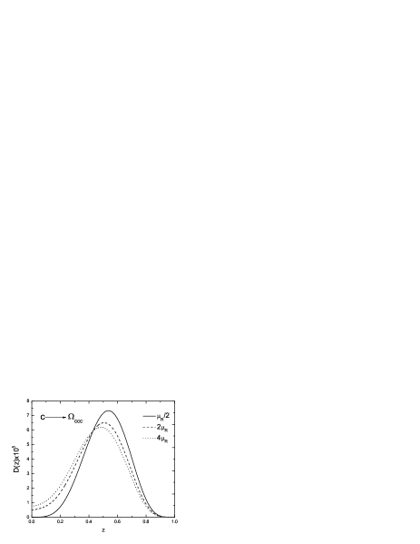
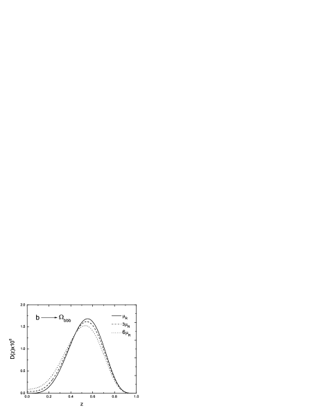
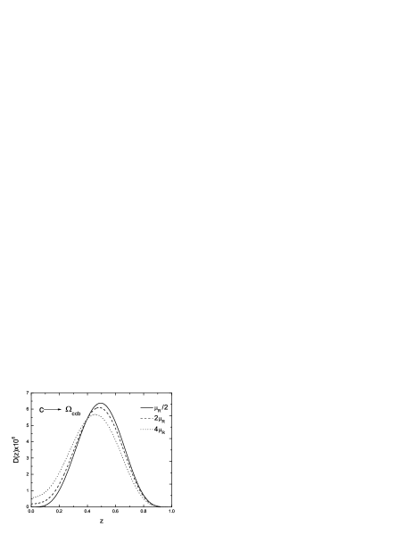
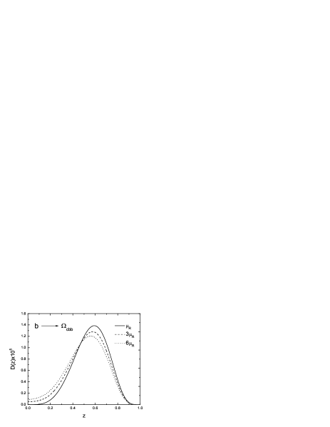
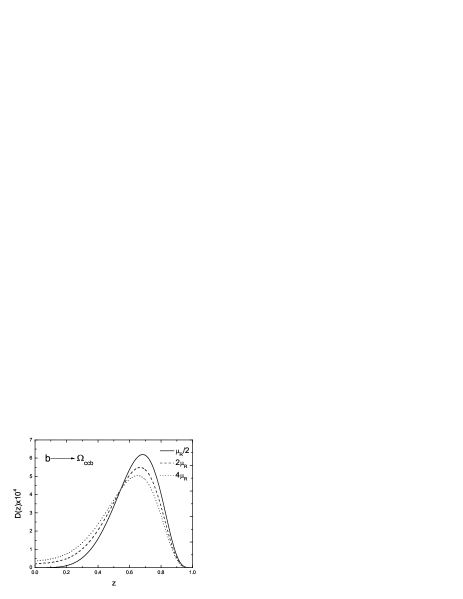
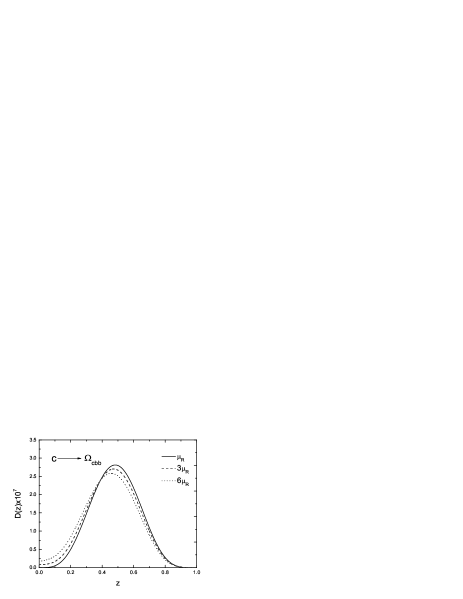
Figure 5: Fragmentation of a $c$ and $b$ quark into possible triply heavy baryons. Note that they are grouped according to their heavy contents. Evolution to desired scales are shown for the LHC. We have used two sets of scales $\mu=\mu_{R}/2,\;2\mu_{R},\;4\mu_{R}$ (left) and $\mu=\mu_{R},\;3\mu_{R},\;6\mu_{R}$ (right).

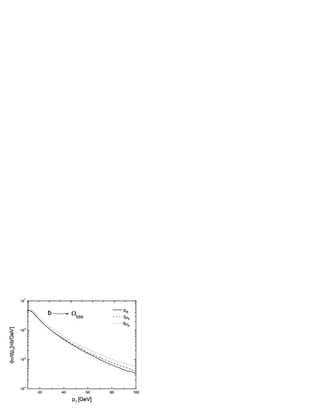
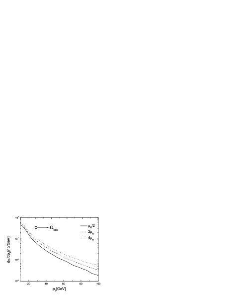
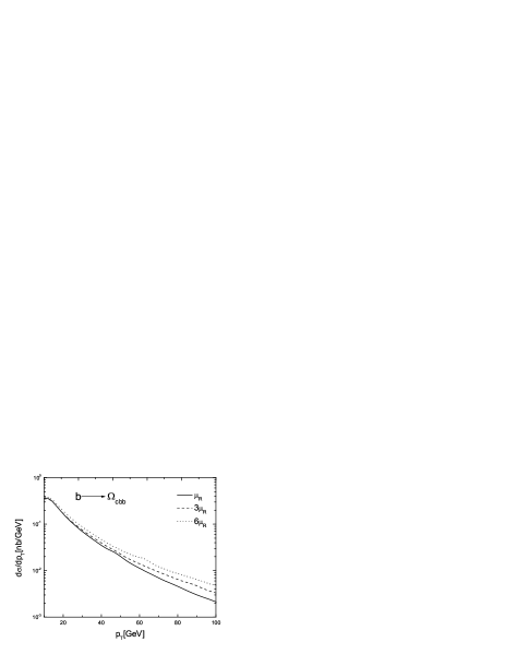
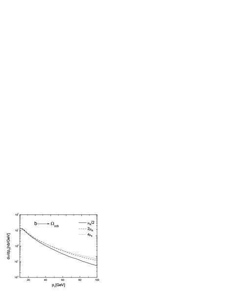
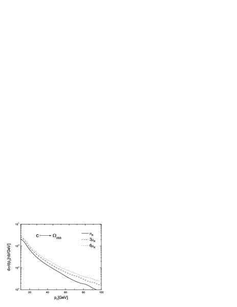
Figure 6: Differential cross section ${\rm d}\sigma/{\rm d}p_{T}[{\rm nb/(GeV)}]$ versus transverse momentum $p_{T}$ for production of different triply heavy baryons in $c$ and $b$ fragmentation at the LHC. In each graph the distribution is shown for scales specified. Note that the sets of scale used in each column of diagrams is the same (the baryons in the left column contain at least two $c$ and in the right column at least two $b$ quark). The kinematical cuts imposed are ${p_{T}}^{\rm cut}>10$ GeV and$|y|\leq 1$.

VI Results and discussion

In the heavy quark limit we have obtained exact analytical fragmentation functions for S-wave triply heavy baryons using leading order perturbative QCD. The non-petubative part of the bound state is treated by employing a delta function type distribution function thus ignoring the respective motion of the constituents. We have obtained the fragmentation functions for $c\rightarrow\Omega_{ccb}$ and $b\rightarrow\Omega_{ccb}$ at the scale of $\mu_{\circ}=m+m_{Q^{\prime}}+m_{Q^{\prime\prime}}$ where $m$ is the baryon mass and ${Q^{\prime}}$ and ${Q^{\prime\prime}}$ are specified in Fig. 1. The functions for $c\rightarrow\Omega_{cbb}$ and $b\rightarrow\Omega_{cbb}$ are obtained simply by the interchange of $c\leftrightarrow b$ in agreement with direct calculations. The fragmentation functions for $c\rightarrow\Omega_{ccc}$ and $b\rightarrow\Omega_{bbb}$ are obtained by setting the $c$ and $b$ quark masses to be equal.

With our choice of quark masses, i.e. $m_{c}$=1.25 GeV, $m_{b}$=4.25 GeV and $\mu_{R}$ defined by (46) the behavior of fragmentation functions as well as the transverse momentum distributions of the differential cross sections are well analyzed if we put the triply heavy baryons in two groups. Those which contain at least two $c$ and those at least two $b$ quarks. Therefore while we need to study the $c\rightarrow\Omega_{ccc}$, $c\rightarrow\Omega_{ccb}$, $b\rightarrow\Omega_{ccb}$ within a lower set of $\mu=\mu_{R}/2,\;2\mu_{R}$ and $4\mu_{R}$ scales, $b\rightarrow\Omega_{bbb}$, $b\rightarrow\Omega_{cbb}$, $c\rightarrow\Omega_{cbb}$ would require higher set of $\mu=\mu_{R},\;3\mu_{R}$ and $6\mu_{R}$. This also provides a means by which the sensitivity of the results are tested. When the first (out of the three selected) scale $\mu=\mu_{R}/2$ ($\mu=\mu_{R}$) is less than $\mu_{\circ}$, which incidently happens for all of our particles, we choose the larger of ($\mu,\;\mu_{\circ}$).

The behavior of our fragmentation functions along with their evolutions at $\mu=\mu_{R}/2$ ($\mu_{R}$), $2\mu_{R}$ ($3\mu$ and $4\mu_{R}$ ($6\mu)$ using the Altarelli-Parisi evolution equation (47) are shown in figure 5 for different $\Omega$ states. Note that the scales used here in each diagram are the same as the ones which are employed in $p_{T}$ distribution diagrams in Fig. 6. Also note that each column of diagrams are sketched in separate set of scales. The universal fragmentation probabilities and the average fragmentation parameters at $\mu_{\circ}$ are shown in table I. The probabilities at this table indicate that while some of the states would have considerable event rates at existing colliders, others are less probable. Therefore here we present their cross sections at the LHC at $\sqrt{s}$=14 TeV.

The differential cross sections are shown in figure 6. The slow fall off of the distributions is expected in the framework of our study. We are dealing with a collider with large $\sqrt{s}$ and production of heaviest hadrons in the standard model both against a sharp fall off. A look at this figure reveals that firstly the differential cross sections are sensitive for different scales chosen only at high transverse momentum for nearly all states. secondly as the number of the $b$ quark is increased in the state, the differential cross section is less sensitive for higher scales. It is seen in the cases of $b\rightarrow\Omega_{bbb}$, $b\rightarrow\Omega_{cbb}$ and $c\rightarrow\Omega_{cbb}$. This was the main reason to choose two different sets of scales here. Sometimes it happens that the distribution for two different scales cross each other. This occurs for $b\rightarrow\Omega_{bbb}$ at $p_{T}$=20 GeV and for $b\rightarrow\Omega_{cbb}$ at nearly $p_{T}$=15 GeV and $b\rightarrow\Omega_{ccb}$ at $p_{T}$=20 GeV all for the first two scales. This means that rate of decrease in differential cross sections are different in the specified $p_{T}$ region for the two scales.

Table 1: The universal fragmentation probabilities (F.P.) and the average fragmentation parameter $\langle z\rangle$ at fragmentation scale for different $\Omega$ states in possible $c$ and $b$ quark fragmentation.

Process	F.P.	$\langle z\rangle(\mu_{\circ})$
$c\rightarrow\Omega_{ccc}$	$2.789\times 10^{-5}$	0.521
$c\rightarrow\Omega_{ccb}$	$2.475\times 10^{-6}$	0.490
$b\rightarrow\Omega_{ccb}$	$2.183\times 10^{-4}$	0.634
$b\rightarrow\Omega_{bbb}$	$6.459\times 10^{-7}$	0.534
$b\rightarrow\Omega_{cbb}$	$5.290\times 10^{-6}$	0.562
$c\rightarrow\Omega_{cbb}$	$1.086\times 10^{-7}$	0.482

Table 2: Total cross section in pb for triply heavy baryons in possible $c$ and $b$ quark fragmentation for various scales at the LHC with $\sqrt{s}=14{\rm TeV}$ where the kinematical cuts of $p_{T}>10$ GeV and$|y|\leq 1$ are imposed. Note that the cross sections are calculated in two groups of scales, ($\mu=\mu_{R}/2,\;2\mu_{R}$ and $4\mu_{R}$) for lighter $c\rightarrow\Omega_{ccc}$, $c\rightarrow\Omega_{ccb}$ and $b\rightarrow\Omega_{ccb}$ and ($\mu=\mu_{R},\;3\mu_{R}$ and $6\mu_{R}$) for heavier $c\rightarrow\Omega_{cbb}$, $b\rightarrow\Omega_{cbb}$ and $b\rightarrow\Omega_{bbb}$ states. The ratios $\sigma(Q\rightarrow\Omega)/\sigma(Q)$ are given in the last column. They are calculated at $\mu=2\mu_{R}$.

Process of				Cross Section [pb]			The Ratio
Production	$\mu_{R}/2$	$\mu_{R}$	$2\mu_{R}$	$3\mu_{R}$	$4\mu_{R}$	$6\mu_{R}$	$\sigma(Q\rightarrow\Omega)/\sigma(Q)$
$c\rightarrow\Omega_{ccc}$	301.88		306.99		307.59		$1.20\times 10^{-7}$
$c\rightarrow\Omega_{ccb}$	26.58		30.03		29.88		$1.18\times 10^{-8}$
$b\rightarrow\Omega_{ccb}$	2153.08		2155.31		1723.80		$3.61\times 10^{-6}$
$b\rightarrow\Omega_{bbb}$		6.34	6.38	5.77		8.40	$1.36\times 10^{-8}$
$b\rightarrow\Omega_{cbb}$		50.30	34.77	47.78		52.34	$7.43\times 10^{-8}$
$c\rightarrow\Omega_{cbb}$		1.14	1.38	1.47		1.49	$5.41\times 10^{-10}$

The total cross sections are listed in table II for the chosen scales. They range from a few nb to a few pb. The decimal places are not realy significant. They are kept only for the matter of comparison. A short look at table II reveals that although the total cross section for some of the triply heavy baryons are small indeed (order of pb) and their production needs energetic hadron colliders, some others such as $b\rightarrow\Omega_{ccb}$ and $c\rightarrow\Omega_{ccc}$ do possess larger cross sections of the order of nb and may easily be produced at the Tevatron as well. An interesting point in table II is that although the total cross section for some of the particles such as $c\rightarrow\Omega_{ccb}$ and $c\rightarrow\Omega_{cbb}$ increase with increasing $\mu$, but this is not the case for the rest. Our investigation shows that this depends on the range of $\mu$ selected and also on the choice of ${p_{T}}^{\rm cut}$ [20]. We have also calculated the ratio $\sigma(\Omega)/\sigma(Q)$ for different cases. The results appear in the last column of table II. Our evaluation of charm and bottom cross sections at the LHC are 0.25497 mb and 0.46812 mb respectively.

The fragmentation production of doubly heavy baryons studied in [4] by Doncheski et al is interesting in relation to our work. First of all the fact that the Tevatron gives large cross section for charm production is reflected in this work. They have obtained nearly equal cross sections for $\Xi_{cc}$ at the Tevatron and at the LHC. However for $\Xi_{cb}$ and $\Xi_{bb}$ the cross sections are different. They report 430 pb, 215 pb and 16 pb for the Tevatron and 470 pb, 490 pb and 36 pb for the LHC respectively for these states. Although states which we have studied are different, but physically our results are comparable with the above.

We would like at the end discuss the uncertainties of our results. The choice of quark masses will not only alter the fragmentation probabilities, but also the value of $\mu$ and values of $x$ at which the parton distribution functions are evaluated. This will of course be reflected on the total cross sections. We have chosen $m_{c}=1.25$ GeV and $m_{b}=4.25$ GeV which are the optimum values reported [19]. However the slightly higher values of $m_{c}=1.5$ GeV and $m_{b}=4.7$ GeV are also used in the literature. Changes in quark mass will affect the fragmentation functions. In the scheme of our calculation, the fragmentation functions inversely depend on quark mass squared. Therefore increase in quark mass will decrease the probabilities. The other quantity which may depend on quark mass is the baryon decay constant. However the later is not much clear in the case of triply heavy baryons. Taking the explicit mass dependence of our fragmentation functions, we have obtained 18 percent decrease in the cross sections in average, when we use the above mentioned higher values.

There is no data on the baryon decay constant. Theoretically one may solve the Schrödinger like equation to obtain the wave function at the origin for these composite particles with heavy constituents and then relate the wave function at the origin to the baryon decay constant. We have avoided this procedure because of theoretical uncertainties instead have chosen $f_{B}=0.25$ GeV on phenomenological grounds. The final quantity of interest is the color factor. We have calculated this quantity using the simple color line counting rule and have obtained $C_{F}=7/6$ for our propose.

References

(1)[1] J.C. Anjos et al, Phys. Rev. D 56, 394 (1997)
(2)[2] A. Adamov and G.R. Goldstien, Phys. Rev. D 56,
7381 (1997)
(3)[3] ALEPH Collaboration, D. Buskulic et al,
Phys. lett. B 374, 319 (1996); Fermilab E704 Collaboration,
A. Bravar et al, Phys. Rev. Lett. 78, 4003 (1997)
(4)[4]M.A. Doncheski et al, Phys. Rev. D 53, 1247
(1996); V.V. Kiselev et al, Phys. Rev. D 60, 014007-1
(1999)
(5)[5] A.F. Falk et al, Phys. Rev. D 49, 555
(1994); See also [1]
(6)[6] E. Braaten et al, Phys. Rev. D 48, 5049
(1993); E. Braaten et al, Phys. Rev. D 51, 4819
(1995); M.A. Gomshi Nobary and T. O’sati, Mod. Phys. Lett. A 15, 455 (2000)
(7)[7] C. H. Chang and Y. Q. Chen, Phys. Rev. D 46, 3845
(1992)
(8)[8] F. Abe et al, Phys. Rev. Lett. 74, 2626
(1995); S Abachi et al, Phys. Rev. Lett. 74, 2632
(1995)
(9)[9] M.A. Gomshi Nobary J. Phys. G: Nucl. Part. Phys. 27, 21 (2001)
and M.A. Gomshi Nobary et
al, Int. Europhysics Conf.on High Energy Physics, Tampere, 1999
(10)[10] S. P. Baranov, V.L. Slad, Phys. At. Nucl. 67, 829
(2004); A. V. Saleev, arXiv:hep-ph/9906515 v1 26 Jun 1999; and
M.A. Gomshi Nobary, Phys. Lett. B 559, 239 (2003) (An
erratum to this reference is reported in Phys. Lett. B 598,
294 (2004). The correct version may be found in arXiv:
hep-ph/048122 v1 10 Aug 2004)
(11)[11] S. P. Baranov in Ref. [10]
(12)[12] M.A. Doncheski in Ref [4]
(13)[13] M. Nattson et al, SELEX Collab. Phys. Rev. Lett.
89, 112001-1 (2002)
(14)[14]M. Lusignoli et al, phys. lett. B 266, 142
(1991) and Z. Phys. C 51, 549 (1991); C.H. Chang and Yu-Qi
Chen, phys. lett. B 284, 127 (1992); C.H. Chang and Yu-Qi
Chen, Phys. Rev. D 46, 3845 (1992); K. Cheung Phys. Rev.
Lett. 71, 3413 (1993); C.H. Chang and Yu-Qi Chen, Phys. Rev.
D 48, 4086 (1993); C.H. Chang et al, Phys. Rev. D 54, 4344 (1996); A.Y. Anisimov, phys. lett. B 452, 129
(1999); V. Kiselev et al, Phys. Rev. D 60, 014007
(1999)
(15)[15] M. Suzuki, Phys. Rev. D 33, 676 (1986)
(16)[16] G. P. Lapage and S. Brodsky. Phys. Rev. D 22, 2
(1980); S. Brodsky and C.R. Ji, Phys. Rev. Lett. 55, 2257
(1985);
(17)[17] A.D. Martin, R.G. Roberts and W.J. Stiriling, Phys. Rev. D 50, 6734 (1994)
(18)[18] P. Nason, S Dawson and R.K. Ellis, Nucl. Phys. B 303, 607
(1988); W.Beenakker, H. Kuijf, W.L.Van Neerven and J. Smith, Phys.
Rev. D 40, 54 (1989); W.Beenakker, W.L.Van Neerven, R.Meng,
G. Schuler and J. Smith, Nucl. Phys. B 351, 507 (1991)
(19)[19]Review of Particle Physics, Phys. Rev. D 66, Number 1-I (2002)
(20)[20]See also: K. Cheung and R.J. Oakes, Phys. Rev. D 53, 1242 (1996)