UCB-PTH-04/19

LBNL-49279

SCIPP-2004/05

Localized Supersoft Supersymmetry Breaking

Z. Chacko^a,b, Patrick J. Fox^c and Hitoshi Murayama^a,b,d

^aDepartment of Physics, University of California, Berkeley, CA 94720, USA
^b Theoretical Physics Group, Lawrence Berkeley National Laboratory,
Berkeley, CA 94720, USA
^c Santa Cruz Institute for Particle Physics, Santa Cruz CA 95064, USA
^d School of Natural Sciences, Institute for Advanced Study, Princeton, NJ 08540, USA

Abstract

We consider supersymmetry breaking models in which the MSSM is extended to include an additional chiral adjoint field for each gauge group with which the the MSSM gauginos acquire Dirac masses. We investigate a framework in which the Standard Model gauge fields propagate in the bulk of a warped extra dimension while quarks and leptons are localized on the ultraviolet brane. The adjoint fields are localized on the infrared brane, where supersymmetry is broken in a hidden sector. This setup naturally suppresses potentially large flavor violating effects, while allowing perturbative gauge coupling unification under SU(5) to be realized. The Standard Model superpartner masses exhibit a supersoft spectrum. Since the soft scalar masses are generated at very low scales of order the gaugino masses these models are significantly less fine-tuned than other supersymmetric models. The LSP in this class of models is the gravitino, while the NLSP is the stau. We show that this theory has an approximate R symmetry under which the gauginos are charged. This symmetry allows several possibilities for experimentally distinguishing the Dirac nature of the gauginos.

1 Introduction

While supersymmetry is the most attractive solution to the hierarchy problem it nevertheless introduces several naturalness puzzles of its own. Chief among them is the ‘supersymmetric flavor problem’ – why do the squark masses conserve flavor? Solutions to the supersymmetric flavor problem have come in two forms – either the squark masses have a renormalization group invariant form that is nearly flavor diagonal at low scales[1, 2, 3, 4] or the squark masses are finite and flavor diagonal at the scale at which they are generated (for example,[5, 6, 7]).

Recently a new and attractive solution to this problem that falls into the latter category has been proposed [8]. In this approach the MSSM is extended to include a new chiral adjoint, often referred to as an “Extended Superpartner” (ESP), for each SM gauge group and an additional U(1$)^{\prime}$ vector superfield under which the MSSM fields are all singlets. The D component of this new U(1$)^{\prime}$ is non-zero, breaking supersymmetry. In such “Gauge Extended Models” (GEMs) each MSSM gaugino acquires a Dirac mass with its corresponding adjoint through a superpotential interaction involving this new U(1$)^{\prime}$ vector superfield. The scalar superpartners acquire their masses from loop diagrams that involve the gauginos and the adjoints and which are dominated by momenta of order the gaugino masses. The scalar masses are finite, loop suppressed with respect to the gaugino masses and flavor diagonal at the matching scale. This pattern of superpartner masses is called supersoft. The fact that in this scenario the gauginos are Dirac makes this an interesting alternative to the conventional MSSM framework with Majorana gauginos.

In GEMs where the dominant source of supersymmetry breaking is the non-zero D-term of a new vector superfield it is important to understand if there are other effects which could cause the superpartner masses to deviate from the supersoft form. Before addressing this question let us first understand the origin of the supersoft contributions. The superpotential operator that generates the gaugino masses has the form

$$\int d^{4}x\int d^{2}\theta\sqrt{2}\frac{W_{\alpha}^{\prime}W^{\alpha}A}{M}+\mbox{h.c.}$$ (1)

where $W_{\alpha}^{\prime}$ is the gauge field strength of the hidden sector vector superfield whose D-component VEV $\left\langle{D^{\prime}}\right\rangle$ breaks supersymmetry, $W_{\alpha}$ is the gauge field strength of a Standard Model vector superfield and $A$ is its corresponding ESP. This leads to a Dirac gaugino mass $M_{D}\approx\;\left\langle{D^{\prime}}\right\rangle/M$. The same interaction results in supersoft scalar masses of order

$$m_{Q}^{2}\approx\frac{g^{2}}{16\pi^{2}}M_{D}^{2}$$ (2)

at one loop order.

Now if $M$ is of order the Planck scale, $M_{Pl}$, then realistic phenomenology requires that $\sqrt{\left\langle{D^{\prime}}\right\rangle}\approx 10^{11}$ GeV. Since the natural size of any Fayet-Iliopoulos term is expected to be of order $M_{Pl}\approx 10^{18}$ GeV [9] the more natural way to generate a non-zero VEV, $\left\langle{D^{\prime}}\right\rangle$, of the right size is to dynamically generate VEVs for a pair of fields $P$ and $\bar{P}$ that are charged under the new U(1$)^{\prime}$. If these VEVs $\left\langle{P}\right\rangle$ and $\left\langle{\bar{P}}\right\rangle$ (and their difference) are of order $10^{11}$ GeV then $\left\langle{D^{\prime}}\right\rangle$ naturally has the right size. This however immediately leads to a problem - operators of the form

$$\int d^{4}x\int d^{4}\theta\;\frac{P^{\dagger}e^{V^{\prime}}P\;Q^{\dagger}Q}{M^{2}}$$ (3)

which are allowed by all the symmetries of the theory give potentially flavor violating contributions to the masses of the MSSM squarks $\tilde{Q}$ which are larger than the supersoft contributions.

Can such flavor violating effects be avoided? One possibility is that the operator of Eqn. (1) which gives rise to gaugino masses only arises at loop level after integrating out heavy fields at some intermediate scale $M$. However, as was shown in [8], the operator

$$\int d^{2}\theta\frac{{W^{\alpha}}^{\prime}W_{\alpha}^{\prime}A^{2}}{M^{2}}+\mbox{h.c.}$$ (4)

is then typically generated at the same loop order. Although this operator does not give divergent contributions to the soft scalar masses it is nevertheless problematic. It gives a negative contribution to the mass squared of either the scalar or pseudoscalar component of the adjoint superfield that is larger (by a loop factor) than the Dirac gaugino mass squared. If there is no other source of supersymmetry breaking for $A$ a supersymmetric mass term for the adjoint superfield

$$\int d^{2}\theta M_{A}A^{2}$$ (5)

must be added to the theory to avoid charge and color breaking vacua. Although this leads an acceptable superparticle spectrum, since $M_{A}$ is significantly larger than $M_{D}$ the Dirac character of the gauginos is lost, and the spectrum of the model tends toward that of intermediate scale gaugino mediation [10],[11].

From this discussion it is clear that the simplest models of Dirac gauginos based on the scenario outlined in [8] do not solve the supersymmetric flavor problem. What can be done to remedy the situation? The approach we will take is to consider a five dimensional space where the MSSM matter fields and the fields $P$ and $\bar{P}$ are localized on different 3-branes. Then the operator of Eqn. (3) is forbidden by locality [1]. Within such a framework there remain two distinct possibilities; one is that the MSSM gauge fields propagate in the bulk of the extra dimension while the other is that they too are localized on a brane with the MSSM matter fields while the U(1$)^{\prime}$ propagates in the bulk. The phenomenological implications of these two possibilities are NOT in fact the same. In what follows we concentrate on the case where the MSSM gauge fields are in the bulk of the space as this offers some significant advantages over the other case, specifically in regard to electroweak symmetry breaking and coupling constant unification. We now explain these advantages.

In models with a supersoft superpartner spectrum obtaining electroweak symmetry breaking is typically not simple. The reason is that in the limit of Dirac gaugino masses (which corresponds to $M_{A}\rightarrow 0$ above), the D-terms which give rise to the Higgs quartic potential vanish, and therefore the tree level Higgs mass vanishes. Additional contributions to the Higgs mass from stop loops can give rise to realistic phenomenology even for $M_{A}<<M_{D}$, but only if the stops are very heavy, which tends to push up the entire spectrum of masses leading to fine-tuning. In our extra dimensional scenario however, if the gauge fields are in the bulk the scalar adjoints can be localized to the brane where supersymmetry is broken. This allows them to directly acquire tree level supersymmetry breaking masses from the operator

$$\int d^{5}x\sqrt{-G}\delta\left(y-\pi R\right)\int d^{4}\theta\;\frac{P^{\dagger}e^{V^{\prime}}P\;A^{\dagger}A}{M_{5}^{4}}$$ (6)

Now that the scalar adjoints are heavy the Higgs quartic potential takes its familiar MSSM form, allowing for more natural electroweak symmetry breaking. The low scale at which the supersoft scalar masses are generated means that the negative correction to the Higgs soft masses from stop loops does not get a large logarithmic enhancement. Therefore the fine-tuning required to obtain electroweak symmetry breaking is significantly less than in, for example, the constrained MSSM.

Another advantage of the higher dimensional scenario with bulk gauge fields relates to gauge coupling unification. Gauge coupling unification must proceed differently in this class of models even in four dimensions because of the additional adjoints. For unification under SU(5) the SU(3), SU(2) and U(1) adjoints $A$ must appear at low energies as part of a complete adjoint of SU(5). However the presence of all these additional fields at low scales makes the gauge couplings sufficiently large before unification is achieved that the predictivity of the model is destroyed. (This difficulty can be avoided if the unifying group is $SU(3)^{3}$, in which case the extra matter content is small enough to allow perturbative unification [8].) The higher dimensional scenario, however, admits perturbative unification under SU(5) if the fifth dimension is warped [12] and the extra adjoints localized to the infrared brane (along with the U(1$)^{\prime}$ gauge field) while the gauge symmetry is broken on the ultraviolet brane. This is because in such a scenario the adjoint fields do not contribute to running above the infrared cutoff. Proton decay can be avoided by having the chiral matter of the MSSM on the ultraviolet brane, which implies that supersymmetry must be broken on the infrared brane in order to avoid the flavor violating operators of Eqn. (3), and to allow the operator of Eqn. (6). We see that the three requirements of unification under SU(5), a flavor diagonal sparticle spectrum and the absence of rapid proton decay together tightly constrain the locations of the various fields in the higher dimensional space.

What are the distinguishing characteristics of this class of models? Since the scale at which supersymmetry is broken is warped down the LSP in this class of models is the gravitino while the NLSP is usually the (right-handed) stau. A very interesting feature of this class of models is that they possesses an approximate R symmetry under which the gaugino and antigaugino have opposite charges. An important consequence of this symmetry is that even though the gauginos are relatively heavy it may nevertheless be straightforward to experimentally distinguish them from Majorana gauginos provided the staus are stable on collider timescales. The reason is that decays of pair produced superparticles nearly always result in oppositely charged staus in the final state if the gauginos are Dirac whereas the staus often have the same charge if the gauginos are Majorana. Even if the staus are not stable on collider time scales it may still be possible to distinguish between Dirac and Majorana gauginos by accurately measuring the charges and energies of the muon and two taus produced in smuon decays. These measurements enable the charge of the decaying smuon to be related to that of the resulting (short-lived) stau - these almost always have the same charge if the gauginos are Dirac. In the sections which follow we explain our model in greater detail.

2 The Framework

In this section we establish the framework we will be working in and the notation we are using. We consider a five dimensional setup. We employ a coordinate system $x^{M}$ where $M$ runs from 0 to 3 and 5. The fifth dimension $x^{5}=y$ is compactified on the interval $0\leq y\leq\pi R$, which can be thought as arising from the orbifold $S^{1}/Z_{2}$. There are 3-branes at the orbifold fixed points $y=0$ and $y=\pi R$ on which fields are localized. The metric is given by the line element

$$ds^{2}=G_{MN}dx^{M}dx^{N}=e^{-2\sigma}\eta_{\mu\nu}dx^{\mu}dx^{\nu}+dy^{2}~{}.$$ (7)

Here the $x^{\mu}$, where $\mu$ runs from 0 to 3, parametrize our usual four spacetime dimensions, $\eta_{\mu\nu}={\rm{diag}}(-1,1,1,1)$, and $\sigma=k\left|y\right|$, where $k$ is the AdS curvature and is related to the four dimensional Planck scale $M_{4}$ and the five dimensional Planck scale $M_{5}$ by

$$M_{4}^{2}=\frac{M_{5}^{3}}{2k}\left(1-e^{-2k\pi R}\right)\simeq\frac{M_{5}^{3}}{2k}~{},$$ (8)

where the second equality holds when the warping is significant.

For what follows we will need to understand the couplings of supersymmetric bulk vector multiplets and bulk hypermultiplets [13]. An on shell vector multiplet in five dimensional ${\cal{N}}=1$ supergravity consists of a gauge field $A_{M}$, a pair of symplectic Majorana spinors $\lambda^{i}$, with $i=1,2$, and a real scalar $\Sigma$ which transforms in the adjoint representation. The bosonic part of the higher dimensional gauge field action takes the form

$$S_{b}=-\int d^{4}x\int dy\sqrt{-G}\frac{1}{g_{5}^{2}}\left[\frac{1}{4}F_{MN}F^{MN}+\frac{1}{2}D_{M}\Sigma\;D^{M}\Sigma+\left(\sigma^{\prime\prime}-2k^{2}\right)\Sigma^{2}\right]~{},$$ (9)

where $\sigma^{\prime\prime}=2k\left[\delta(y)-\delta(y-\pi R)\right]$. The fermionic part takes the form

$$S_{f}=-\int d^{4}x\int dy\sqrt{-G}\frac{i}{2g_{5}^{2}}\left[\bar{\lambda}^{i}\Gamma^{M}D_{M}\lambda^{i}+\frac{1}{2}\sigma^{\prime}\bar{\lambda}^{i}\left(\sigma^{3}\right)^{ij}\lambda^{j}\right]~{},$$ (10)

where $D_{M}$ is a covariant derivative with respect to both general coordinate and gauge transformations. The vielbein factors necessary to write the spinor action in curved space are implicit in Eqn. (10).

We demand that $A_{\mu}$ and $\lambda^{1}_{L}$ are even while $\Sigma$ and $\lambda^{2}_{L}$ are odd. Then the even fields each have a massless mode with the following $y$ dependence:

$$A_{\mu}\left(x,y\right) = \frac{1}{\sqrt{\pi R}}A_{\mu}^{\left(0\right)}\left(x\right)+\cdots$$ (11)

$$\lambda^{1}_{L}\left(x,y\right) = \frac{e^{3\sigma/2}}{\sqrt{\pi R}}\lambda^{1\;\left(0\right)}_{L}\left(x\right)+\cdots$$ (12)

The lightest KK masses are of order $M_{c}=k\,e^{-k\pi R}$, which we will call the compactification scale. We are interested in compactification scales larger than the scale of supersymmetry breaking but much smaller than the unification scale $\approx 10^{16}$GeV.

A bulk hypermultiplet $H$ consists of two complex scalars $\phi^{i}$ and a Dirac fermion $\psi$. The bulk action has the form

$$S_{H}=-\int d^{4}x\int dy\sqrt{-G}|\partial_{M}\phi^{i}|^{2}+i\bar{\psi}\Gamma^{M}D_{M}\psi+m_{\phi,i}^{2}|\phi^{i}|^{2}+im_{\psi}\bar{\psi}\psi$$ (13)

where the five dimensional masses of the scalars and the fermion are constrained to satisfy

$$m_{\phi,i}^{2} = \left(c^{2}\pm c-\frac{15}{4}\right)k^{2}+\left(\frac{3}{2}\mp c\right)\sigma^{\prime\prime}$$ (14)

$$m_{\psi} = c\sigma^{\prime}$$ (15)

Here $c$ is a dimensionless number that can be chosen arbitrarily. We demand that $\phi^{1}$ and $\psi_{L}$ are even, while $\phi^{2}$ and $\psi_{R}$ are odd. Then each even field has a massless mode with a profile given by

$$\phi^{1}\left(x,y\right) = {e^{\left(3/2-c\right)\sigma}}\phi\left(x\right)$$ (16)

$$\psi_{L}\left(x,y\right) = {e^{\left(2-c\right)\sigma}}\psi\left(x\right)$$ (17)

For $c=1/2$, the kinetic terms are independent of the extra coordinate, just as the zero modes of the bulk vector multiplet.

3 The Model

In this section we describe our model in detail. We are interested in a scenario where the Standard Model quark, lepton and Higgs fields are localized on the brane at $y=0$ where the warp factor is large and the local scale is $\sim M_{GUT}$ while supersymmetry is broken on the brane at $y=\pi R$ where the warp factor is small and the local scale is $\sim M_{IR}$. The MSSM gauge fields live in the bulk and couple to both the matter fields localized on the ultraviolet brane, and to the supersymmetry breaking sector which is localized on the infrared brane. We assume that the grand unifying symmetry, which is SU(5), is broken on the UV brane by the Higgs mechanism. The ESPs $A_{i}$ are also localized on the infrared brane. Since the SU(5) symmetry is unbroken there these form a complete SU(5) multiplet. The interaction which gives the gauginos a mass takes the familiar supersoft form

$$\int d^{5}x\sqrt{-G}\;\delta\left(y-\pi R\right)\int d^{2}\theta\sqrt{2}\frac{W_{\alpha}^{\prime}W_{i}^{\alpha}A_{i}}{M_{5}}$$ (18)

where $W_{i}$ is the field strength, for the $i^{th}$ gauge group, formed from the even components of the bulk gauge supermultiplet. $W^{\prime}$ is the field strength of the U(1$)^{\prime}$ gauge field which is localized on the IR brane and whose D component $\left\langle{D^{\prime}}\right\rangle$ breaks supersymmetry. This leads to a gaugino mass

$$M_{D,i}(\mu)=\frac{\left\langle{D^{\prime}}\right\rangle}{M_{5}}e^{-k\pi R}\left[\frac{\alpha_{i}(\mu)}{\alpha_{i}(M_{IR})}\right]^{\frac{b_{i}-2c_{i}}{2b_{i}}}\left[\alpha_{i}(M_{IR})\right]^{1/2},$$ (19)

where $b_{i}=-(3N_{c}-N_{f})$ is the coefficient of the beta function for the gauge coupling $g_{i}$ and $c_{i}$ is the quadratic Casimir of the gauge representation, $c_{i}=(N^{2}-1)/2N$ for a fundamental representation. In the limit that the the infrared scale is very close to the weak scale each gaugino mass is proportional to its corresponding gauge coupling. Note that here $\left\langle{D^{\prime}}\right\rangle$ is defined as a scale in the 5D theory. In the effective 4D theory this scale is warped down, Eqn.(40).

The MSSM scalar superpartners acquire a supersoft contribution to their soft masses that arises at loop level from the gaugino mass $M_{D}$. This contribution is finite and given by [8],

$${m^{2}}_{i,SS}(\mu)=\frac{c_{i}\alpha_{i}M_{D,i}^{2}(\mu)}{\pi}\log\left(4+\frac{m_{\tilde{A}}^{2}}{M_{D,i}^{2}(\mu)}\right)$$ (20)

where $M_{D,i}$ is the mass of the gaugino of the $i$th gauge group and $m_{\tilde{A}}^{2}$ is the mass² of the scalar adjoint.

We assume for the purposes of this model that the non-zero VEV $\left\langle{D^{\prime}}\right\rangle$ is generated dynamically as the difference in the VEVs of a pair of fields $P$ and $\bar{P}$ which have opposite charges under the U($1)^{\prime}$. This is more natural than employing a Fayet-Iliopoulos term. If there are no unnaturally small parameters in this sector we expect $\left\langle{P}\right\rangle\;\approx\;\left\langle{\bar{P}}\right\rangle\;\approx\;\sqrt{\left\langle{D^{\prime}}\right\rangle}$. The scalar component of the adjoint field A can then directly pick up a soft mass ${m_{\tilde{A}}}^{2}$ from the interaction

$$\int d^{5}x\sqrt{-G}\;\delta\left(y-\pi R\right)\int d^{4}\theta\frac{P^{\dagger}e^{V^{\prime}}PA^{\dagger}A}{M_{5}^{2}}$$ (21)

Since this arises directly at tree level and has no large volume suppression we expect that the scalar components of the adjoint will be relatively heavy. This soft mass for the scalar adjoints feeds back into the soft masses of the MSSM scalars at two loops through gauge interactions [21].

$$\Delta{m^{2}}\approx-\left(\frac{g^{2}}{16\pi^{2}}\right)^{2}{m_{\tilde{A}}}^{2}{\rm log}\left(\frac{ke^{-k\pi R}}{m_{\tilde{A}}}\right)$$ (22)

This term can give sizable corrections to the soft scalar masses that are comparable to the supersoft contribution. A ‘Naive Dimensional Analysis’ (NDA) estimate (see the appendix) suggests that the size of these corrections can naturally be limited to about 20% of the supersoft contribution. If however the infrared scale is high, the logarithm becomes important and mild finetuning may be needed.

Another potential contribution to the soft scalar masses arises from hard supersymmetry breaking operators localized on the infrared brane. These have the form

$$\int d^{5}x\sqrt{-G}\;\delta\left(y-\pi R\right)\int d^{4}\theta\frac{W^{\alpha}D^{2}W_{\alpha}\;P^{\dagger}e^{V^{\prime}}P}{M_{5}^{4}}$$ (23)

The effect of this and analogous operators is to alter the relative couplings of gauge bosons and gauginos to matter. In the context of higher dimensional models similar operators were considered in [22]. They cannot be forbidden by any symmetry, and generate flavor diagonal scalar masses at one loop. However an NDA estimate suggests that these corrections are small compared to the supersoft contribution, as shown in the appendix.

Yet another potential contribution to the soft scalar masses arises from the kinetic mixing between U(1)^′ and U(1)_Y gauge fields. If it is unsuppressed,

$$\int d^{5}x\sqrt{-G}\;\delta\left(y-\pi R\right)\int d^{2}\theta\ W^{\prime}_{\alpha}W_{Y}^{\alpha},$$ (24)

will induce a large $D_{Y}\approx D$ for $U(1)_{Y}$ and contributions to scalar masses $\Delta m_{i}^{2}=g^{\prime 2}Y_{i}D_{Y}$. It overcomes the one-loop supersoft contributions of Eq. (20), and hence some of the scalar masses become negative. Our model avoids this problem with the SU(5) invariance on the IR brane that does not allow for this kinetic mixing. Because U(1)^′ is localized on the IR brane and there is no possible counter term, there is no logarithmically divergent radiative effects either. We conclude the model is immune to this potential disaster.

Since the supersymmetry breaking scale is relatively low the LSP in these models will be the gravitino. The NLSP will be the right handed stau, which we expect to be somewhat lighter than the other right handed sleptons. The large soft mass of the scalar adjoints implies that the Higgs quartic terms are not suppressed as in minimal supersoft models. The relevant part of the scalar Lagrangian is

$$L_{S}=-M_{D}(\tilde{A}+\tilde{A^{*}})D-D\left(\Sigma_{i}\;g\;q^{*}_{i}Tq_{i}\right)-\frac{1}{2}D^{2}-{m_{\tilde{A}}}^{2}\left(\tilde{A}\tilde{A^{*}}\right)$$ (25)

From this it is straightforward to infer that the Higgs quartic term is the same as in the MSSM upto corrections of order $M_{D}^{2}/m_{\tilde{A}}^{2}$. Pushing $m_{\tilde{A}}$ high allows EWSB to go through as in the MSSM but for large infrared scale this reintroduces the problem of large negative contributions to the soft scalar massed squared, Eqn.(22). When minimising the Higgs potential in subsequent sections we take into account the small correction to the quartic coming from the triplet and singlet ESP scalars. For the purposes of this paper we treat $\mu$ and $B\mu$ as free input parameters and do not specify a dynamical origin for them. It may be possible to generate suitable values for these parameters from the VEV of a singlet which lives in the bulk and communicates directly with the supersymmetry breaking sector. However we do not pursue this possibility further here.

Perturbative gauge coupling unification arises naturally in this model, even under SU(5). The SU(3), SU(2) and U(1) ESPs are now extended to a complete adjoint of SU(5). The GUT group, which for concreteness we take to be SU(5), is assumed to be broken on the ultraviolet brane. As has recently been established, gauge couplings run logarithmically in AdS spaces [23, 25, 26, 27, 28, 24, 29, 30]. Since the adjoint field is localized on the infrared brane its contribution to running is SU(5) symmetric and cutoff at the compactification scale, while the brane-localized gauge couplings on the ultraviolet brane which do not respect SU(5) unify at the GUT scale.

An additional interaction is required to give a mass to the fermions in the adjoint of SU(5) that are not adjoints of SU(3), SU(2) or U(1) . The scalar adjoints all acquire a mass from the supersymmetry breaking interaction above while the fermions that are adjoints under SU(3), SU(2) and U(1) acquire Dirac masses with the gauginos. One possibility is to write a mass term

$$\int d^{5}x\sqrt{-G}\;\delta\left(y-\pi R\right)\int d^{2}\theta M_{A}A^{2}$$ (26)

on the infrared brane. Since such a term is necessarily SU(5) symmetric this will result in a mass for the SU(3), SU(2) and U(1) adjoint fermions as well with the result that the gauginos are no longer purely Dirac. However provided $M_{A}$ is sufficiently smaller than $M_{D}$ the gauginos will still be pseudo-Dirac. As with $\mu$ and $B\mu$, for the purposes of this paper we treat $M_{A}$ as a free parameter and do not specify a dynamical origin for it.

In the absence of the $\mu$, $B\mu$ and $M_{A}^{2}$ terms in the Lagrangian the theory has an exact continuous R-symmetry under which all the chiral superfields of the MSSM have charge 1 and the adjoint superfield $A$ and Higgs fields have charge 0. This approximate symmetry has several important consequences. Since any A-term for the MSSM fields breaks this symmetry it can only be generated by loops involving these couplings.

This approximate R symmetry also leads to very interesting experimental signals for the Dirac gauginos in this class of models. Since the gauginos are relatively heavy it might have been expected that it would be extremely difficult to distinguish them from Majorana gauginos. However this is not the case if the NLSP, which is the stau, is long lived. Consider the decay of a pair of superparticles that have been pair produced in a collider (Figures 1 and 2). Each of these will eventually decay into a stau-tau pair primarily through an off-shell bino. However since the bino and anti-bino have opposite R-charges each of the two staus that is produced will always have opposite sign charge relative to the other as will to its associated tau. This is in sharp contrast to the case where the gauginos are Majorana. Here, since a gaugino Majorana mass term breaks the R symmetry, the two staus could have the same charge. The staus are unstable and each will decay into a tau and a gravitino. The stau lifetime depends on the supersymmetry breaking scale $\sqrt{D^{\prime}}$. If the staus are stable on collider time-scales their charges can be determined. This seems a very promising approach to distinguish Dirac gauginos from Majorana gauginos in this class of models.

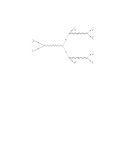
Figure 1: Signal of Dirac gauginos at a leptonic collider.

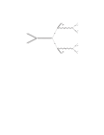
Figure 2: Signal of Dirac gauginos at a hadronic collider.

Since in our model the R-symmetry is not exact the gauginos are therefore only pseudo-Dirac, the staus will sometimes have the same charge. The frequency with which this occurs depends on the ratio of the mass of the SU(5)/SU(3)$\times$SU(2)$\times$U(1) adjoints to the gaugino mass. When this ratio is very small the gauginos tend to be purely Dirac.

However in some models the supersymmetry breaking scale may be too low and therefore the stau lifetime too short to allow the charges of the staus to be determined. We now argue that it may nevertheless be possible to distinguish Dirac gauginos from Majorana gauginos even in such a scenario. A key observation is that in these models the mass splitting between the right-handed sleptons is in general rather small. Consider then the decay of a right-handed smuon that has been produced in a collider into a muon, a tau and a stau through an (off-shell) bino. The Dirac nature of the gauginos implies that the stau has the same charge as the decaying smuon, as does the muon. The small mass splitting between the smuon and the stau means that in the smuon rest frame the muon and the tau both have small momenta. However in this frame the tau produced by the prompt decay of the stau has a large momentum, and carries the same charge as the stau. If the energies and charges of the smuon decay products can be accurately determined in the laboratory frame, then by boosting back to the (approximate) smuon rest frame it may be possible to distinguish between the two taus. We can then determine if the smuon and the stau had the same charge, and therefore (given enough events) if the gauginos are Majorana or Dirac.

At lepton colliders Dirac and Majorana gauginos can also be distinguished by using polarized beams. The approximate R-symmetry of these models implies that the cross-sections for $e^{+}e^{-}\rightarrow$ 2 superparticles and also $e^{-}e^{-}\rightarrow$ 2 superparticles are very small unless the incident leptons have opposite helicities. Therefore a measurement of the cross-section to two superparticles for different helicities of the incident leptons may be sufficient to distinguish between the two cases.

For values of the supersymmetry breaking scale $\sqrt{\left\langle{D^{\prime}}\right\rangle}\;e^{-k\pi R}$ greater than about 3$\times 10^{6}$ GeV the stau NLSPs are sufficiently long lived that it may be possible to detect these particles in neutrino telescopes [32],[33]. Very high energy neutrinos originating from astrophysical sources can collide with nuclei inside the earth, producing a pair of superparticles which promptly decay to staus. These staus can be seen in neutrino telescopes as a pair of parallel charged tracks emerging from the earth about 100m apart. Interestingly, the Dirac nature of the gauginos in these models means that the expected number of events is somewhat less than for Majorana gauginos even for the same superparticle spectrum. The reason is that the R-symmetry restricts the helicities of the incident (anti)neutrino and (anti)quark in these processes to be opposite, while for the case of Majorana gauginos there is no such restriction. Given enough events and some knowledge of the superpartner spectrum, this may be another way to experimentally distinguish between Dirac and Majorana gauginos.

3.1 Sample Spectra

In the table below we give some sample spectra for this class of models. For simplicity we do not incorporate a dynamical origin for the $\mu$ and $B\mu$ terms but merely treat them as free input parameters. The top Yukawa, $y_{t}$ is defined at the IR scale as is the gaugino mass parameter, $m_{g}\equiv(D^{\prime}/M_{5})e^{-k\pi R}$. For simplicity the supersymmetric mass term for the ESPs $M_{A}$ and the soft scalar mass for the ESPs $m_{\tilde{A}}$ are given at 1 TeV. For each set of inputs the superpartner mass spectrum is calculated, the masses are given at 1 TeV. The two sets of inputs, A and B, correspond to an IR scale of 1000 TeV and 30 TeV respectively.

The deviation from the conventional MSSM Higgs potential is determined by the magnitude of $M_{D}/m_{\tilde{A}}$, and has been included in the spectrum. The size of the negative Poppitz-Trivedi contribution to scalar mass squared relative to the supersoft contribution is set by the same parameter, and also by $\log M_{IR}/m_{\tilde{A}}$. For the points B the Poppitz-Trivedi corrections are small and can be ignored. For the points A we do not include them but they can have a sizeable effect. In both cases we include the effect of the the ESPs on the Higgs potential, in particular the suppression of the quartic term.

The final row in Table 1 measures the sensitivity of the Higgs VEV to changes in $\mu$. We search parameter space for regions where the input parameters give correct EWSB with a Higgs VEV of 174 GeV. At these points we measure our sensitivity as,

$$\kappa\equiv\frac{\mu}{v}\frac{\partial v}{\partial\mu}.$$ (27)

The sensitivity is clearly less than in typical high scale models of supersymmetry breaking, for which $\kappa$ usually lies between 50 and 200. Therefore these supersoft models are significantly less fine-tuned than most supersymmetric models.

There are several general features of the spectrum we would like to emphasise. The gauginos are pseudo-Dirac with small, $\mathcal{O}(M_{A})$, splittings. Colored particles are all heavier than 1.5 TeV and yet the Higgs mass can still be light. The stop loops that feed into the Higgs mass are cutoff by the gluino mass rather than the usual GUT/Planck scale since the mass for a colored scalar is only generated at the gluino mass. This finiteness property means we no longer have a log sensitivity to the GUT scale, which is why these models are less fine-tuned than models where the scalar masses are generated at high scales.

		Point A	Point A′	Point B	Point B′
inputs:	$m_{g}$	$14\times 10^{3}$	$18\times 10^{3}$	$15\times 10^{3}$	$21\times 10^{3}$
	$m_{\tilde{A}}$	$8.7\times 10^{3}$	$16\times 10^{3}$	$16\times 10^{3}$	$22\times 10^{3}$
	$M_{A}$	$300$	$300$	$300$	$300$
	$y_{t}$	1	1	1.05	1.05
neutralinos:	$m_{\chi^{0}_{1}}$	426.1	556.0	323.8	446.6
	$m_{\chi^{0}_{2}}$	426.3	556.1	324.0	446.7
	$m_{\chi^{0}_{3}}$	1730	2240	1886	2611
	$m_{\chi^{0}_{4}}$	2030	2540	2186	2911
	$m_{\chi^{0}_{5}}$	2619	3371	2723	3748
	$m_{\chi^{0}_{6}}$	2918	3671	3023	4048
charginos:	$m_{\chi^{\pm}_{1}}$	426.4	556.2	324.0	446.7
	$m_{\chi^{\pm}_{2}}$	2617	3370	2722	3748
	$m_{\chi^{\pm}_{3}}$	2917	3670	3022	4048
Higgs:	$\tan\beta$	5.21	4.33	3.57	3.61
	$m_{h^{0}}$	119.4	127.7	117.1	124.6
	$m_{H^{0}}$	598.5	814.8	608.2	831.8
	$m_{A}$	597.5	813.6	606.0	830.2
	$m_{H^{\pm}}$	602.8	817.6	611.3	834.0
	$\mu$	426.4	556.2	324.0	446.8
	$B$	155.0	260.7	294.6	397.1
sleptons:	$m_{\tilde{e}_{R}}$	199.6	273.8	242.5	328.4
	$m_{\tilde{e}_{L}}$	407.1	569.5	490.4	667.4
	$m_{\tilde{\nu}_{L}}$	401.8	564.4	484.8	663.3
stops:	$m_{\tilde{t}_{1}}$	1749	2393	1855	2526
	$m_{\tilde{t}_{2}}$	1708	2335	1860	2450
other squarks:	$m_{\tilde{u}_{L}}$	1740	2386	1847	2549
	$m_{\tilde{u}_{R}}$	1699	2339	1792	2445
	$m_{\tilde{d}_{L}}$	1741	2388	1849	2520
	$m_{\tilde{d}_{R}}$	1696	2324	1787	2438
gluino:	$M_{3}$	6285	7998	5623	7634
sensitivity:	$\kappa$	25	38	15	26

Table 1: Sample points in parameter space, all masses are in GeV. The A points have $M_{IR}=10^{6}$GeV and the B points have $M_{IR}=30\times 10^{3}$ GeV.

4 Conclusions

We have constructed models of supersoft supersymmetry breaking with Dirac gauginos in which the breaking of supersymmetry is localized to a brane in a higher dimensional space. These theories have three significant advantages over the corresponding models in four dimensions -

• natural suppression of potentially dangerous flavor violating operators

• more natural electroweak symmetry breaking

• the possibility of grand unification under SU(5).

In these theories the lightest supersymmetric particle is the gravitino, while the next to lightest supersymmetric particle is the stau. The spectra exhibit the characteristic supersoft relations among the superparticle masses. In general the squarks and gauginos tend to be fairly heavy, with masses of order a few TeV, while the sleptons are much lighter. In spite of these large squark masses the degree of fine-tuning required to obtain electroweak symmetry breaking is significantly better than in most other supersymmetric models. The reason is that the scalar masses are generated only at very low scales of order the gaugino masses, and hence the negative correction to the Higgs soft mass squared from stop loops does not have a large logarithmic enhancement. The large radiative correction to the quartic term in the Higgs potential from the heavy stops also partially compensates for the reduced contribution to the quartic from the SU(2)_L and U(1)_Y D-terms that is a characteristic of supersoft models.

Even if the gauginos are too heavy to be produced on shell an approximate R-symmetry of these models implies that if the stau is stable on collider time-scales the Dirac nature of the gauginos can be probed. The reason is that decays of heavy superpartners almost always lead to opposite sign staus in the final state if the gauginos are Dirac, while this is not true for Majorana gauginos. Even if the stau is not stable on collider time scales it may still be possible to distinguish between Dirac and Majorana gauginos by accurately measuring the charges and energies of the muon and two taus produced in smuon decays. These measurements enable the charge of the decaying smuon to be related to that of the resulting (short-lived) stau - these almost always have the same charge if the gauginos are Dirac.

Acknowledgements

ZC would like to thank Ian Hinchliffe for useful discussions. PF would like to thank Neal Weiner and David E. Kaplan for useful discussions. PF is supported in part by the U.S. Department of Energy. Z.C. and H.M. were supported in part by the Director, Office of Science, Office of High Energy and Nuclear Physics, of the U.S. Department of Energy under Contract DE-AC03-76SF00098 and DE-FG03-91ER-40676, and in part by the National Science Foundation under grant PHY-00-98840. The work of H.M. was also supported by the Institute for Advanced Study, funds for Natural Sciences.

Appendix A Warped Naive Dimensional Analysis

Consider a scenario where a theory becomes strongly coupled at some fundamental scale $\Lambda$. Loop effects are now no longer suppressed relative to tree level effects at this scale. The methods of ‘Naive Dimensional Analysis’ (NDA) [34, 35] can then be used to estimate the relative strengths of the various couplings in the theory. Since the geometrical factors present in loop calculations determine the suppression of quantum effects relative to classical effects the condition that all interactions are strong at the fundamental scale is dependent on the number of dimensions that the fields of the theory propagate in. NDA in the context of extra dimensions was first studied in [36]. Here we are interested in NDA in warped extra dimensions. We will be interested in cases where the cutoff $\Lambda$ is larger than the curvature scale $k$. This means that the parameters of the theory are determined by physics at much shorter distances than the curvature scale. Therefore the only effect of the warping is that the local cutoff $\Lambda e^{-ky}$ will now vary as a function of location in the fifth dimension. These assumptions of NDA lead to a Lagrangian of the form below.

$$S\sim\int d^{5}x\sqrt{-g}\left(\frac{\Lambda^{5}}{\epsilon\,l_{5}}\hat{\mathcal{L}}_{\mathrm{bulk}}(\hat{\Phi},\frac{\partial}{\Lambda})+\delta(y-y_{\mathrm{brane}})\frac{\Lambda^{4}}{\epsilon\,l_{4}}\hat{\mathcal{L}}_{\mathrm{brane}}(\hat{\Phi},\hat{\phi},\frac{\partial}{\Lambda})\right).$$ (28)

Here $l_{D}=2^{D}\pi^{D/2}\Gamma(D/2)$ is the loop factor in $D$ dimensions. The parameter $\epsilon$ [7] is a measure of the amplitudes of one loop processes relative to tree level processes, or more generally (N+1) loop processes relative to N loop processes. $\epsilon$ lies in the range $0\leq\epsilon\leq 1$ with $1$ being the strong coupling limit and $0$ being the free theory. Hatted fields are dimensionless and all the couplings in $\hat{\mathcal{L}}_{\mathrm{bulk}}$ and $\hat{\mathcal{L}}_{\mathrm{brane}}$ are order one at the high scale.

We now wish to determine the sizes of various parameters in the theory. In going from the 5 dimensional action to the effective 4 dimensional theory it is necessary to take into account the $y$ profile of the bulk fields. One simplification that occurs in the case of bulk gauge fields is that due to 4 dimensional gauge invariance the gauge boson zero-mode is flat in the extra dimension. SUSY is unbroken at the compactification scale so the gaugino acquires a profile such that the whole gauge action is $y$ independent. Therefore gauge and gaugino zero modes behave like flat space zero modes.

Let us first relate the strong coupling scale to the 5 dimensional Planck scale. Recall the Einstein-Hilbert action in 5 dimensions,

$$\int d^{5}x\sqrt{-g}M_{5}^{3}R,$$ (29)

where $R$ contains 2 derivatives of the metric. Comparing this to Eqn. (28) we see that

$$\frac{\Lambda^{3}}{\epsilon\,l_{5}}=M_{5}^{3}.$$ (30)

A similar analysis can be carried out to relate the bulk gauge coupling to the effective 4 dimensional gauge coupling. The zero mode gauge field action is (schematically) given by,

$$S\sim\int d^{4}xdy\frac{\Lambda^{5}}{\epsilon\,l_{5}}\left(\left(\frac{\partial}{\Lambda}\hat{A}^{(0)}\right)^{2}+\frac{\partial}{\Lambda}\hat{A}^{(0)3}+\hat{A}^{(0)4}\right),$$ (31)

due to gauge invariance there is no dependence on the $y$ coordinate. In canonical normalization the 4 dimensional gauge fields are given by,

$$A_{\mu}\sim\left(\frac{\Lambda^{3}2\pi R}{\epsilon l_{5}}\right)^{1/2}\hat{A}^{(0)}_{\mu},$$ (32)

and so the 4 dimensional gauge coupling is given by,

$$g_{4}^{2}=\frac{\epsilon\,l_{5}}{2\pi\Lambda R}.$$ (33)

We demand that the 4D gauge coupling is order one and that the extra dimension is large enough that the infrared scale is order $1$ TeV, i.e. $k\pi R\sim 30$. Using these relations along with Eqn.(8) gives,

$$M_{4}^{2}\sim\frac{\Lambda^{2}}{30}.$$ (34)

It will be useful to know the ratio $k/\Lambda$ which is,

$$\frac{k}{\Lambda}\sim\frac{30}{\epsilon\,l_{5}}\sim\frac{1}{25\epsilon}.$$ (35)

By definition $\epsilon<1$, in addition we require $k/\Lambda<1/4$ placing lower limits on $\epsilon$. Thus, $\epsilon$ lies in the range $1/6<\epsilon<1$ and $1/25<k/\Lambda<1/4$. Now we discuss the relative sizes of the various SUSY breaking effects with the NDA assumption.

First consider the supersoft operator that generates the Dirac gaugino masses. The relevant piece of the action is given by,

$$S \sim \int d^{5}x\sqrt{-g}\left[\frac{\Lambda^{5}}{\epsilon\,l_{5}}\int\frac{d^{2}\theta}{\Lambda}\hat{W}_{\alpha}\hat{W}^{\alpha}+\delta(y-\pi R)\frac{\Lambda^{4}}{\epsilon\,l_{4}}\left(\int\frac{d^{2}\theta}{\Lambda}\hat{W}^{\prime}_{\alpha}\hat{W}^{\prime\alpha}\right.\right.$$ (37)

$$\left.\left.+\int\frac{d^{2}\theta}{\Lambda}\hat{W}_{\alpha}^{\prime}\hat{W}^{\alpha}\hat{A}+\int\frac{d^{4}\theta}{\Lambda^{2}}\hat{A}^{\dagger}\hat{A}\right)\right]$$

$$\sim \int d^{4}x\frac{2\pi R\Lambda^{5}}{\epsilon l_{5}}\hat{\lambda}\frac{\partial}{\Lambda}\hat{\lambda}+\frac{\Lambda^{4}}{\epsilon\,l_{4}}e^{-4\sigma(\pi R)}\left(e^{3\sigma(\pi R)/2}\hat{D}^{\prime}\hat{\lambda}\hat{\psi}_{A}+\hat{D}^{\prime 2}\right.$$ (39)

$$\left.+e^{\sigma(\pi R)}\hat{\bar{\psi}}_{A}\frac{\partial}{\Lambda}\hat{\psi}_{A}\right)+\ldots,$$

where in the second line we have inserted the $y$ profiles of the fields and integrated over the extra dimension. Rescaling fields so that they are canonically normalized and using the fact that the four dimensional gauge coupling is order 1, Eqn.(33), the Dirac mass term is,

$$M_{D}\sim e^{\sigma(\pi R)}\frac{\overline{D}}{\Lambda}\lambda\psi_{A}.$$ (40)

Note that $\overline{D}=D^{\prime}e^{-2\sigma(\pi R)}$. Here $\overline{D}$ should be thought of as the VEV in warped down units and $D^{\prime}$ is the VEV in the 5D theory where all mass scales are defined at the 5D Planck scale. This Dirac gaugino mass in turn gives supersoft contributions to the scalar masses at one loop,

$$m_{SS}^{2}\sim\frac{1}{l_{4}}\left(\frac{\overline{D}}{\Lambda}\right)^{2}e^{2\sigma(\pi R)}.$$ (41)

The non-zero $D$-term VEV is generated from a VEV for the fields $P$ and $\bar{P}$ charged under the $U(1)^{\prime}$. We can relate the sizes of the $\overline{D}$ and $\langle P\rangle$ by considering the operator $\hat{P}^{\dagger}e^{\hat{V}^{\prime}}\hat{P}$ and rescaling $\hat{P}$ to give it canonical kinetic term to find,

$$\langle\overline{D}\rangle=\sqrt{\epsilon\,l_{4}}\langle P\rangle^{2}.$$ (42)

Hard SUSY breaking operators of the form (23) localised on the UV brane can alter the relative couplings of gauginos and gauge bosons to matter. These in turn generate flavour diagonal corrections to the scalar masses at one loop. We now estimate the size of these corrections using NDA. The operator we consider is,

$$\int d^{5}x\sqrt{-g}\delta(y-\pi R)\frac{\Lambda^{4}}{\epsilon\,l_{4}}\int\frac{d^{4}\theta}{\Lambda^{2}}\hat{P}^{\dagger}e^{\hat{V}^{\prime}}\hat{P}\hat{W}_{\alpha}\frac{D^{2}}{\Lambda}\hat{W}^{\alpha}.$$ (43)

In terms of canonically normalized fields the correction to the gaugino kinetic term is,

$$\frac{\overline{D}^{2}}{\Lambda^{4}}e^{4\sigma(\pi R)}\lambda\partial\lambda.$$ (44)

This is a correction to the gauge coupling, $1/g^{2}\rightarrow 1/g_{0}^{2}+(\overline{D}e^{{2\sigma(\pi R)}}/\Lambda^{2})^{2}$. This leads to a one loop quadratically divergent contribution to the scalar mass which is cutoff at the mass of the lightest KK state. So,

$$m_{HB}^{2}=\frac{1}{l_{4}}\left(\frac{\overline{D}}{\Lambda^{2}}\right)^{2}e^{4\sigma(\pi R)}g_{4}^{4}\left(ke^{-\sigma(\pi R)}\right)^{2}=\frac{1}{l_{4}}\left(\frac{\overline{D}}{\Lambda}\right)^{2}\left(\frac{k}{\Lambda}\right)^{2}e^{2\sigma(\pi R)},$$ (45)

which is smaller than the supersoft contribution by a factor of $\left(k/\Lambda\right)^{2}\sim\left(1/25\epsilon\right)^{2}$.

There is a two loop logarithmically divergent correction to the soft scalar masses arising from the soft mass for the adjoint Eqn.(21), as shown in  [21]. The logarithm is cut-off close to the mass of the lightest KK state. This correction will be negative provided the logarithm is larger than order unity. The operator that leads to the adjoint soft mass has the form

$$\int d^{5}x\sqrt{-g}\delta(y-\pi R)\int\frac{d^{4}\theta}{\Lambda^{2}}\hat{P}^{\dagger}e^{\hat{V}^{\prime}}\hat{P}\hat{A}^{\dagger}\hat{A}\rightarrow\epsilon\,l_{4}e^{2\sigma(\pi R)}\frac{\overline{D}^{2}}{\Lambda^{2}}A^{2}$$ (46)

The leading contribution to the scalar mass is [21],

$$m_{\tilde{q}}^{2}\sim-\frac{1}{l_{4}}\epsilon\left(\frac{\overline{D}}{\Lambda}\right)^{2}e^{2\sigma(\pi R)}\log\frac{ke^{-\sigma(\pi R)}}{M_{D}}$$ (47)

Finally we wish to know the size of the other possible supersoft operator, $W^{\prime}_{\alpha}W^{\prime\alpha}A^{2}$, this operator splits the mass squared of the real and imaginary parts of the adjoint scalar, pushing one positive and one negative. Using NDA the size can be estimated,

$$\int d^{5}x\sqrt{-g}\delta(y-\pi R)\int\frac{d^{2}\theta}{\Lambda^{2}}\frac{\hat{W}^{\prime}_{\alpha}\hat{W}^{\prime\alpha}}{\Lambda^{2}}\hat{A}^{2}.\rightarrow\epsilon l_{4}\left(\frac{\overline{D}}{\Lambda}\right)^{2}e^{2\sigma(\pi R)}A^{2}$$ (48)

Notice that this is the same size as the positive contribution from Eqn.(46), so that both the real and imaginary component of each scalar adjoint can naturally have a net positive mass squared.

References

- [1] L. Randall and R. Sundrum, Nucl. Phys. B 557, 79 (1999) [arXiv:hep-th/9810155].
- [2] G. F. Giudice, M. A. Luty, H. Murayama and R. Rattazzi, JHEP 9812, 027 (1998) [arXiv:hep-ph/9810442].
- [3] I. Jack and D. R. T. Jones, Phys. Lett. B 482, 167 (2000) [arXiv:hep-ph/0003081]; I. Jack and D. R. T. Jones, Phys. Lett. B 491, 151 (2000) [arXiv:hep-ph/0006116].
- [4] N. Arkani-Hamed, D. E. Kaplan, H. Murayama and Y. Nomura, JHEP 0102, 041 (2001) [arXiv:hep-ph/0012103].
- [5] M. Dine, W. Fischler and M. Srednicki, Nucl. Phys. B 189, 575 (1981); S. Dimopoulos and S. Raby, Nucl. Phys. B 192, 353 (1981); L. Alvarez-Gaume, M. Claudson and M. B. Wise, Nucl. Phys. B 207, 96 (1982); M. Dine and A. E. Nelson, Phys. Rev. D 48, 1277 (1993) [arXiv:hep-ph/9303230]; M. Dine, A. E. Nelson and Y. Shirman, Phys. Rev. D 51, 1362 (1995) [arXiv:hep-ph/9408384]; M. Dine, A. E. Nelson, Y. Nir and Y. Shirman, Phys. Rev. D 53, 2658 (1996) [arXiv:hep-ph/9507378].
- [6] D. E. Kaplan, G. D. Kribs and M. Schmaltz, Phys. Rev. D 62, 035010 (2000) [arXiv:hep-ph/9911293];
- [7] Z. Chacko, M. A. Luty, A. E. Nelson and E. Ponton, JHEP 0001, 003 (2000) [arXiv:hep-ph/9911323].
- [8] P. J. Fox, A. E. Nelson and N. Weiner, JHEP 0208, 035 (2002) [arXiv:hep-ph/0206096].
- [9] W. Fischler, H. P. Nilles, J. Polchinski, S. Raby and L. Susskind, Phys. Rev. Lett. 47, 757 (1981).
- [10] C. Csaki, J. Erlich, C. Grojean and G. D. Kribs, Phys. Rev. D 65, 015003 (2002) [arXiv:hep-ph/0106044].
- [11] H. C. Cheng, D. E. Kaplan, M. Schmaltz and W. Skiba, Phys. Lett. B 515, 395 (2001) [arXiv:hep-ph/0106098].
- [12] L. Randall and R. Sundrum, Phys. Rev. Lett. 83, 3370 (1999) [arXiv:hep-ph/9905221].
- [13] T. Gherghetta and A. Pomarol, Nucl. Phys. B 586, 141 (2000) [arXiv:hep-ph/0003129]
- [14] T. Gherghetta and A. Pomarol, Nucl. Phys. B 602, 3 (2001) [arXiv:hep-ph/0012378]; D. Marti and A. Pomarol, Phys. Rev. D 64, 105025 (2001) [arXiv:hep-th/0106256];
- [15] W. D. Goldberger, Y. Nomura and D. R. Smith, Phys. Rev. D 67, 075021 (2003) [arXiv:hep-ph/0209158].
- [16] K. w. Choi, D. Y. Kim, I. W. Kim and T. Kobayashi, arXiv:hep-ph/0301131;
- [17] Z. Chacko and E. Ponton, JHEP 0311, 024 (2003) [arXiv:hep-ph/0301171];
- [18] K. w. Choi, D. Y. Kim, I. W. Kim and T. Kobayashi, arXiv:hep-ph/0305024;
- [19] Y. Nomura and D. R. Smith, Phys. Rev. D 68, 075003 (2003) [arXiv:hep-ph/0305214].
- [20] Y. Nomura, D. Tucker-Smith and B. Tweedie, arXiv:hep-ph/0403170.
- [21] E. Poppitz and S. P. Trivedi, Phys. Lett. B 401, 38 (1997) [arXiv:hep-ph/9703246].
- [22] D. E. Kaplan and G. D. Kribs, JHEP 0009, 048 (2000) [arXiv:hep-ph/0009195].
- [23] A. Pomarol, Phys. Rev. Lett. 85, 4004 (2000) [arXiv:hep-ph/0005293].
- [24] W. D. Goldberger and I. Z. Rothstein, Phys. Lett. B 491, 339 (2000) [arXiv:hep-th/0007065]; W. D. Goldberger and I. Z. Rothstein, Phys. Rev. Lett. 89, 131601 (2002) [arXiv:hep-th/0204160]; W. D. Goldberger and I. Z. Rothstein, Phys. Rev. D 68, 125011 (2003) [arXiv:hep-th/0208060].
- [25] L. Randall and M. D. Schwartz, JHEP 0111, 003 (2001) [arXiv:hep-th/0108114]; L. Randall and M. D. Schwartz, Phys. Rev. Lett. 88, 081801 (2002) [arXiv:hep-th/0108115];
- [26] K. Agashe, A. Delgado and R. Sundrum, Nucl. Phys. B 643, 172 (2002) [arXiv:hep-ph/0206099]; K. Agashe and A. Delgado, Phys. Rev. D 67, 046003 (2003) [arXiv:hep-th/0209212]; K. Agashe, A. Delgado and R. Sundrum, Annals Phys. 304, 145 (2003) [arXiv:hep-ph/0212028].
- [27] K. w. Choi, H. D. Kim and Y. W. Kim, JHEP 0211, 033 (2002) [arXiv:hep-ph/0202257]. K. w. Choi, H. D. Kim and I. W. Kim, JHEP 0303, 034 (2003) [arXiv:hep-ph/0207013]; K. w. Choi and I. W. Kim, Phys. Rev. D 67, 045005 (2003) [arXiv:hep-th/0208071].
- [28] R. Contino, P. Creminelli and E. Trincherini, JHEP 0210, 029 (2002) [arXiv:hep-th/0208002];
- [29] A. Falkowski and H. D. Kim, JHEP 0208, 052 (2002) [arXiv:hep-ph/0208058].
- [30] L. Randall, Y. Shadmi and N. Weiner, JHEP 0301, 055 (2003) [arXiv:hep-th/0208120].
- [31] A. E. Nelson, TASI Lectures, 2002.
- [32] I. Albuquerque, G. Burdman and Z. Chacko, arXiv:hep-ph/0312197.
- [33] X. J. Bi, J. X. Wang, C. Zhang and X. m. Zhang, arXiv:hep-ph/0404263.
- [34] A. Manohar and H. Georgi, Nucl. Phys. B 234, 189 (1984). H. Georgi and L. Randall, Nucl. Phys. B 276, 241 (1986).
- [35] M. A. Luty, Phys. Rev. D 57, 1531 (1998) [arXiv:hep-ph/9706235]. A. G. Cohen, D. B. Kaplan and A. E. Nelson, Phys. Lett. B 412, 301 (1997) [arXiv:hep-ph/9706275].
- [36] Z. Chacko, M. A. Luty and E. Ponton, JHEP 0007, 036 (2000) [arXiv:hep-ph/9909248].