Transport equations for chiral fermions to order $\hbar$

and electroweak baryogenesis: Part II

Tomislav Prokopec^⋄, Michael G. Schmidt^⋄

and Steffen Weinstock^∙

^⋄ Institut für Theoretische Physik, Universität Heidelberg
Philosophenweg 16, D-69120 Heidelberg, Germany

^∙ Nuclear Theory Group, Brookhaven National Laboratory, Upton, NY 11973-5000, USA

Abstract

This is the second in a series of two papers. While in Paper I PSW_1 we derive semiclassical Boltzmann transport equations and study their flow terms, here we make use of the results from that paper and address the collision terms. We use a model Lagrangean, in which fermions couple to scalars through Yukawa interactions and approximate the self-energies by the one-loop expressions. This approximation already contains important aspects of thermalization and scatterings required for quantitative studies of transport in plasmas. We compute the CP-violating contributions to both the scalar and the fermionic collision term. CP-violating sources appear at order $\hbar$ in gradient and a weak coupling expansion, as a consequence of a CP-violating split in the fermionic dispersion relation. These represent the first controlled calculations of CP-violating collisional sources, thus establishing the existence of ‘spontaneous’ baryogenesis sources in the collision term. The calculation is performed by the use of the spin quasiparticle states established in Paper I. Next, we present the relevant leading order calculation of the relaxation rates for the spin states and relate them to the more standard relaxation rates for the helicity states. We also analyze the associated fluid equations, and make a comparison between the source arising from the semiclassical force in the flow term and the collisional source, and observe that the semiclassical source tends to be more important in the limit of inefficient diffusion/transport.

^⋄T.Prokopec@, M.G.Schmidt@thphys.uni-heidelberg.de
^∙weinstock@bnl.gov

1 Introduction

This is the second part in a series of two closely related papers, where we study the emergence of Boltzmann transport equations from quantum field theory for particles with a space-time dependent mass, which often arises via a coupling to a varying background field. This setting is typically realised at phase transitions, an important example being electroweak scale baryogenesis, in which case particles acquire mass at the electroweak phase transition through the Higgs mechanism. This paper is an immediate continuation of Paper I PSW_1 , to which we refer for a general introduction and motivation. We frequently refer to sections and equations of Paper I, and indicate this by adding a prefix “I.” to the respective reference.

We work in a model (I.2.13-I.2.14) with chiral fermions $\psi_{L,R}$ that couple to scalars $\phi$ via a Yukawa interaction ${\cal L}_{\rm int}$ (see Eq. (20) below):

$${\cal L} = i\bar{\psi}\mathbin{\partial\mkern-10.5mu\big{/}}\psi-\bar{\psi}_{L}m\psi_{R}-\bar{\psi}_{R}m^{*}\psi_{L}+\left(\partial_{\mu}\phi\right)^{\dagger}\left(\partial^{\mu}\phi\right)-\phi^{\dagger}M^{2}\phi+{\cal L}_{\rm int}\,.$$ (1)

Due to the interaction with some background field the masses $m$ and $M^{2}$ are space-time dependent, and they may contain complex elements to allow for CP-violation. In Paper I, based on a 2PI effective action we derive the Schwinger-Dyson equations for this system, from which we arrive at the Kadanoff-Baym equations (I.2.54-I.2.55) for the scalar and fermionic Wightman functions $\Delta^{<,>}$ and $S^{<,>}$, which in the Wigner representation read

$$\Big{(}k^{2}-\frac{1}{4}\partial^{2}+ik\cdot\partial-M^{2}{\rm e}^{-\frac{i}{2}\stackrel{{\scriptstyle\leftarrow}}{{\partial}}\cdot\partial_{k}}\Big{)}\Delta^{<,>}-{\rm e}^{-i\diamond}\{\Pi_{h}\}\{\Delta^{<,>}\}-{\rm e}^{-i\diamond}\{\Pi^{<,>}\}\{\Delta_{h}\}={\cal C}_{\phi}$$ (2)

$$\Big{(}\mathbin{k\mkern-9.8mu\big{/}}+\frac{i}{2}\mathbin{\partial\mkern-10.5mu\big{/}}-m_{h}{\rm e}^{-\frac{i}{2}\stackrel{{\scriptstyle\leftarrow}}{{\partial}}\cdot\,\partial_{k}}-i\gamma^{5}m_{a}{\rm e}^{-\frac{i}{2}\stackrel{{\scriptstyle\leftarrow}}{{\partial}}\cdot\,\partial_{k}}\Big{)}S^{<,>}-{\rm e}^{-i\diamond}\{\Sigma_{h}\}\{S^{<,>}\}-{\rm e}^{-i\diamond}\{\Sigma^{<,>}\}\{S_{h}\}={\cal C}_{\psi}\,,$$ (3)

where $\Pi^{<,>}$, $\Pi_{h}$ ($\Sigma^{<,>}$, $\Sigma_{h}$) denote the scalar (fermionic) self-energies. The scalar and fermionic collision terms are of the form

$${\cal C}_{\phi} = \frac{1}{2}{\rm e}^{-i\diamond}\big{(}\{\Pi^{>}\}\{\Delta^{<}\}-\{\Pi^{<}\}\{\Delta^{>}\}\big{)}$$ (4)

$${\cal C}_{\psi} = \frac{1}{2}{\rm e}^{-i\diamond}\big{(}\{\Sigma^{>}\}\{S^{<}\}-\{\Sigma^{<}\}\{S^{>}\}\big{)}\,,$$ (5)

where $\diamond\{a\}\{b\}\equiv(1/2)(\partial_{x}a\cdot\partial_{k}b-\partial_{k}a\cdot\partial_{x}b)$. In section I.3 we argue that the last two terms on the left hand side of the equations, which represent collisional broadening due to multiparticle effects, can be neglected.

We then show that to first order in gradients (equivalently, to linear order in $\hbar$) the scalar Wigner function is solved by the classical on-shell distribution function (I.4.12)

$$i\Delta^{<}(k,x)=\frac{\pi}{\omega_{\phi}}\left[\delta(k_{0}-\omega_{\phi})-\delta(k_{0}+\omega_{\phi})\right]n^{\phi}(k,x)\,,$$ (6)

where the dispersion relation is given by $\omega_{\phi}=(\vec{k}^{\,2}+M^{2})^{1/2}$. This solution applies to the one field case, but also to the diagonal entries of the Wightman function in the mass eigenbasis in the case with mixing scalars, provided no eigenvalues $M_{i}^{2}$ of $M^{2}$ are nearly degenerate, that is $\hbar k\cdot\partial\ll M_{i}^{2}-M_{j}^{2}\;(\,\forall i,j)$. From (6) it then follows that particle and antiparticle densities are the on-shell projections (I.4.31, I.4.34)

$$f^{\phi}_{+}(\vec{k},x) = n^{\phi}\big{(}\omega_{\phi}(\vec{k},x),\vec{k},x\big{)}$$ (7)

$$f^{\phi}_{-}(\vec{k},x) = n^{\phi cp}\big{(}\omega_{\phi},\vec{k},x\big{)}=-\big{[}1+n^{\phi}\big{(}-\omega_{\phi},-\vec{k},x\big{)}\big{]}\,.$$ (8)

When working to order $\hbar$ accuracy, one gets the following Boltzmann equation for the CP-violating density, $\delta f^{\phi}=f^{\phi}_{+}-f^{\phi}_{-}$ (I.4.36)

$$\left(\partial_{t}+\frac{\vec{k}\cdot{\nabla}}{\omega_{\phi}}-\frac{(\partial_{z}{M^{2}}(z))}{2\omega_{\phi}}\partial_{k_{z}}\!\right)\delta f^{\phi}(\vec{k},x)\!=\!\int_{0}^{\infty}\!\!\frac{dk_{0}}{2\pi}\big{[}{\cal C}_{\phi}(k,x)+{\cal C}^{\dagger}_{\phi}(k,x)+\,{\cal C}_{\phi}(-k,x)+{\cal C}^{\dagger}_{\phi}(-k,x)\big{]}.\quad\;$$ (9)

The discussion of the fermionic kinetic equation in Paper I begins with the observation (see Refs. KainulainenProkopecSchmidtWeinstock:2001 and KainulainenProkopecSchmidtWeinstock:2002 ) that, if masses only depend on the z-coordinate (e.g. caused by planar phase interfaces), the following spin operator (I.5.18)

$$S_{z}(k)=\frac{1}{\tilde{k}_{0}}\left(k_{0}\gamma^{0}-\vec{k}_{\|}\cdot\vec{\gamma}\right)\gamma^{3}\gamma^{5}\,$$ (10)

is a conserved quantity. Here $\tilde{k}_{0}={\rm sign}(k_{0})(k_{0}^{2}-k_{x}^{2}-k_{y}^{2})^{1/2}$ is obtained by boosting $k_{0}$ to a frame, in which $k_{x}$ and $k_{y}$ vanish. With the spin projector $P_{s}(k)=(\mathbbm{1}+sS_{z}(k))/2\;$ $(s=\pm 1)$ the fermionic Wigner function can accordingly be cast to a spin diagonal form (I.5.25)

$$S_{s}=iP_{s}\left[s\gamma^{3}\gamma^{5}g^{s}_{0}-s\gamma^{3}g^{s}_{3}+{\mathbbm{1}}g^{s}_{1}-i\gamma^{5}g^{s}_{2}\right]\,.$$ (11)

In stationary situations the densities $g^{s}_{a}\;(a=0,1,2,3)$ are (real) functions of $z$ and momentum. Only one of these functions is independent. Indeed, by making use of the constraint equations, one can express $g^{s}_{1,2,3}$ in terms of $g^{s}_{0}$.

In Paper I we show that, when the collisional broadening (width) is neglected, quasiparticle picture remains valid to order $\hbar$ (see also KainulainenProkopecSchmidtWeinstock:2001 and KainulainenProkopecSchmidtWeinstock:2002 ), such that the constraint equation for the vector density $g^{s}_{0}$ is solved by the following on-shell form (I.5.71)

$$g_{0}^{<s}(k,x) = 2\pi\sum_{\pm}\frac{\delta(k_{0}\mp\omega_{\pm s})}{2\omega_{\pm s}Z_{\pm s}}\,|\tilde{k}_{0}|\,n_{s}\,,$$ (12)

where $n_{s}=n_{s}(k,x)$ is a distribution function, to be determined by solving the kinetic equation, and $Z_{s}$ is the rate of change of the energy-squared around the poles (divided by $2\omega_{s}$). The dispersion relation $\omega_{s}=\omega_{s}(k,z)$ acquires a CP violating, spin dependent, shift due to the interaction with the background field (I.5.72):

$$\omega_{s}=\omega_{0}-\frac{s}{2\tilde{\omega}_{0}\omega_{0}}|m|^{2}\partial_{z}{\theta}\,.$$ (13)

Here $\theta$ is the phase of the complex mass and $\omega_{0}=(\vec{k}^{2}+|m|^{2})^{\frac{1}{2}},$ $\tilde{\omega}_{0}=(k_{z}^{2}+|m|^{2})^{\frac{1}{2}}.$ The densities of particles and anti-particles with spin $s$ are the on-shell projections (I.5.120-121)

$$f_{s+}(\vec{k},x) = n_{s}(\omega_{s},\vec{k},x)$$ (14)

$$f_{s-}(\vec{k},x) = n^{cp}_{s}(\omega_{s},\vec{k},x)=1-n_{-s}(-\omega_{s},-\vec{k},x)\,.$$ (15)

Besides an equilibrium part and a CP-even deviation from the equilibrium density, these particle densities contain spin dependent contributions $\delta f_{s\pm}$. From these we form two combinations, which are related to vector and axial density (I.5.131-132):

$$\delta f^{v}_{s} \equiv \delta f_{s+}-\delta f_{s-}$$ (16)

$$\delta f^{a}_{s} \equiv \delta f_{s+}-\delta f_{-s-}\,.$$ (17)

While the Boltzmann equation for the vector part does not have a semiclassical source (I.5.133)

$$\big{(}\partial_{t}+\vec{v}_{0}\cdot\nabla_{\vec{x}}+F_{0}\partial_{k_{z}}\big{)}\delta f^{v}_{s}=\int_{0}^{\infty}\frac{dk_{0}}{\pi}\big{(}{\cal K}^{s}_{0}(k)-{\cal K}^{cps}_{0}(k)\big{)}\,,$$ (18)

there is a CP-violating semiclassical source $s{\cal S}^{\rm flow}$ (I.5.135) in the equation for the distribution function related to the axial density (I.5.134):

$$\big{(}\partial_{t}+\vec{v}_{0}\cdot\nabla_{\vec{x}}+F_{0}\partial_{k_{z}}\big{)}\delta f^{a}_{s}+s{\cal S}^{\rm flow}=\int_{0}^{\infty}\frac{dk_{0}}{\pi}\left({\cal K}^{s}_{0}(k)-{\cal K}^{cp-s}_{0}(k)\right)\,,$$ (19)

where $\vec{v}_{0}=\vec{k}/\omega_{0}$ and $F_{0}=-(\partial_{z}|m|^{2})/(2\omega_{0})$. The collisional contributions on the right hand side are essentially the traces of the spin projected fermionic collision term.

In Paper I we formally kept the contributions of the collision term in all expressions, as can be seen in Eqs. (9) and (18,19), but we never evaluated them. This will be done here. In the actual calculations we truncate the self-energies in the collision term at the one-loop order.

Section 2 is devoted to a calculation of CP-violating sources both in the scalar and in the fermionic collision term. We emphasize that this represents the first ever calculation of CP-violating sources arising from nonlocal (loop) effects. It would be incorrect to associate or identify our calculation with, for example, Ref. Riotto:1998 , where the author evaluates the self-energy for stops and charginos by taking account of the contributions from two mass insertions, which represent an approximation of the stop and charginos interactions with the Higgs background. Formally, all mass insertions are to be considered as singular contributions to the self-energy, and hence ought to be viewed as part of the (renormalized) mass term. We emphasize that in the formalism presented here all contributions to the self-energy arising from the mass insertions (resummed) are fully included in the fermion masses in the flow term. Treating mass insertions in any other way is not in the spirit of Kadanoff-Baym equations, and hence it is not guaranteed to yield correct results.

Making use of the Wigner functions obtained in Paper I, in section 2.1 we compute a CP-violating collision source in the scalar kinetic equation. The source originates from the fermionic Wigner functions, which we model by the CP-violating equilibrium solutions accurate to the first order in $\hbar$. The source appears in the fluid continuity equation. We also briefly discuss the case of mixing fermions. This represents a first calculation of a CP-violating source in the scalar kinetic equation, and can be used, for example, for baryogenesis scenarios mediated by scalar particles, e.g. Higgs particles or squarks.

CP-violating collisional sources in the fermionic transport equations are the subject of section 2.2. We calculate the leading order CP-violating source, which appears first when the self-energies are approximated at the one-loop order. The source is of first order in gradients, it is suppressed by the wall velocity, and its parametric dependence is qualitatively different from the semiclassical force source. For example, the collisional source is suppressed by the Yukawa coupling squared, and it exhibits a kinematic mass threshold – it vanishes when $M\leq 2|m|$, where $M$ denotes the scalar mass. Moreover, the source appears in the fluid Euler equation, to be contrasted with the semiclassical force, which sources the continuity equation. The source we compute arises from a nonlocal (one-loop) contribution to the collision term, and it differs qualitatively from the spontaneous baryogenesis sources obtained so far in the literature HuetNelson:1995+1996 ; Riotto:1995 ; Riotto:1998 ; CarenaQuirosRiottoViljaWagner:1997 ; CarenaMorenoQuirosSecoWagner:2000 ; CarenaQuirosSecoWagner:2002 , where the source is computed from the (local) tree level mass insertions.

In order to study equilibration, in section 3 we use a linear response approximation to compute relaxation rates for spin quasiparticles from the one-loop self-energies. When viewed in the Boltzmann collision term, these rates capture an on-shell emission or absorption of a scalar particle by a fermion, such that, as a consequence of the vertex energy-momentum conservation, the rates vanish in the limit of vanishing masses. Moreover, for finite fermion and scalar masses, the rates are kinematically suppressed, illustrating the shortcomings of the one loop approximation to the self-energies. Since the two-loop rates, which include the radiative vertex corrections to the above processes, but also the (off-shell) scalar exchange, do not vanish in the massless limit, they typically dominate relaxation to equilibrium, even when Yukawa couplings are quite small. To calculate these rates in the collision term of the Kadanoff-Baym equations would require an extensive calculational effort, and it is beyond the scope of this work. We begin section 3 by showing that thermalization rates do not depend on whether one uses equilibrium Wigner functions (approximated at leading order in gradients), or the standard spinors (with a definite spin). Next, we point out that in the ultrarelativistic limit the spin rates reduce to the (more standard) helicity rates, provided helicity is identified as the spin in the direction of propagation, which accords with our findings in section LABEL:Kinetics_of_fermions:_tree-level_analysis. This establishes a connection between the relaxation rates for spin and helicity states, which are almost exclusively quoted in literature.

By taking moments of the transport equations obtained in section LABEL:Kinetics_of_fermions:_tree-level_analysis, in section 4 we derive and analyze the fermionic fluid equations for CP-violating densities and velocities. We observe that the continuity equation contains the CP-violating source arising from the semiclassical force, while the Euler equation – which expresses the fluid momentum conservation – contains the collisional source. The earlier works on baryogenesis, which were based on a heuristic WKB approach, have used helicity states, for which the semiclassical source appears in the Euler equation. Of course, helicity states can be obtained by a coherent superposition of spin states, such that, in principle, it should not matter which states one uses. In a quasiparticle picture, however, the information on quantum coherence is lost, and the dynamics of helicity states differ in general from that of spin states. Namely, at the order $\hbar$, the interactions with a CP-violating Higgs background coherently mix the states of opposite helicity, which cannot be described in a quasiparticle picture. Formally, one can combine the Boltzmann equations for different spin and sign of momentum (in the direction of the wall propagation), such that the source in the fluid equations appears in the Euler equation, just as if helicity were conserved. These new equations correspond to taking different moments of the Boltzmann equations. Based on the above comments, it is clear that it would be incorrect to identify these as the fluid equations for quasiparticles of conserved helicity. In fact, this identification becomes legitimate only in the extreme relativistic limit. Taking different moments of the Boltzmann equations, such that the semiclassical source appears in different fluid equations, results formally in a priori equally accurate fluid equations. This observation lead us to conclude that these two sets of equations can be used as a testing ground for the accuracy of fluid equations, which could otherwise be tested only by a comparison with the exact solution of the Boltzmann equation. We perform this test in section 4, and find that the two sets of diffusion equations give results that differ at about 10 percent level. Finally, we show how, starting with fluid equations, one arrives at a diffusion equation which contains both sources, and thus allows for a comparison of the strength of the semiclassical and collisional sources at the one-loop level. Our conclusion is that unless diffusion is very effective the semiclassical force dominates. A more detailed look at the sources and rates from the one-loop collision term analysis indicates a mild suppression of the collisional source with respect to the flow term source. We expect that this suppression persists at higher loops as well. However, to get a more quantitative estimate for the strength – and thus relevance – of the collisional sources, one would have to include the contributions from the two-loop self-energies, which is beyond the scope of this work.

2 Collision term

In Paper I we have considered tree-level interactions of particles in a plasma with spatially dependent scalar and pseudoscalar mass terms. In this section we extend our analysis to include CP-violating contributions from the collision terms of both scalars and fermions. Our study is mainly motivated by an ongoing dispute in literature concerning the question whether the dominant CP-violating sources for electroweak baryogenesis arise from the flow term or from the collision term. While here we present just a first attempt to address this tantalizing question in a controlled manner, we believe that our analysis, which is based on the collision term with the self-energies truncated at one loop, serves as a good indicator for the typical strength of the collisional sources, and may serve as a good guideline for a comparison of the baryogenesis sources from the flow term (semiclassical force) and collisional (spontaneous) sources. Some, but not all, of the results discussed in this section have already been presented at conferences KainulainenProkopecSchmidtWeinstock:2002b ; Prokopec:2002 ; ProkopecKainulainenSchmidtWeinstock:2003 .

The simple picture of collisional baryogenesis is based on the idea of spontaneous baryogenesis CohenKaplanNelson:1991 . According to this idea, since particles and the corresponding CP-conjugate antiparticles with opposite spin see different energy-momentum dispersion relations in the presence of a CP-violating bubble wall, rescatterings have a tendency to preferably populate one type of particle states compared to the other, and thus source a CP-violating current. This current then biases sphalerons, leading to baryon production. This idea has been further developed and adapted to electroweak baryogenesis mediated by supersymmetric particles, mostly charginos and neutralinos of the MSSM HuetNelson:1995+1996 ; Riotto:1995 ; Riotto:1998 ; CarenaQuirosRiottoViljaWagner:1997 ; CarenaMorenoQuirosSecoWagner:2000 ; CarenaQuirosSecoWagner:2002 and NMSSM DaviesFroggattMoorhouse:1996 . This approach is to be contrasted with the semiclassical force mechanism JoyceProkopecTurok:1995 ; JoyceProkopecTurok:1996 ; ClineKainulainen:2000 ; ClineJoyceKainulainen:2000+2001 ; HuberSchmidt:2000 ; HuberSchmidt:2001 ; HuberJohnSchmidt:2001 discussed in detail in Paper I.

In the classical Boltzmann equation the flow term, which is first order in gradients, is balanced by the collision term of zeroth order in gradients, and hence both can formally be considered to be of the order $\hbar^{0}$ in gradient expansion. We shall assume that our truncation of the flow term at second order in gradients (formally at first order in $\hbar$) can be considered equivalent to a truncation of the collision term at first order in gradients, so we will consistently neglect all higher order terms here.

All Wigner functions in our work are on-shell and can eventually be reduced to particle distribution functions (6, 12). These distribution functions can be split up into a thermal distribution, the Bose-Einstein distribution $n^{\phi}_{\rm eq}$ in the scalar case and the Fermi-Dirac distribution $n_{\rm eq}$ for the fermions, and a correction function $\delta n^{\phi}$ and $\delta n$, respectively. Let us for the study of the collision term assume that these deviations from the thermal distributions are suppressed by at least one order in gradients in comparison to them. After expanding the sums $n^{\phi}_{\rm eq}+\delta n^{\phi}$ and $n_{\rm eq}+\delta n$ in the collision term, we can organize the contributions into two groups: those which contain correction functions, and those which only contain the equilibrium distributions. The terms in the first group are the relaxation terms one usually finds on the right hand side of a Boltzmann equation. They try to drive the deviations to zero and vanish for $\delta n^{\phi}=\delta n=0$. We will study them in more detail in section 3. The terms of the second group owe their presence to the fermionic Wigner function, which contains first order effects besides the non-thermal distributions. These terms are present even for $\delta n^{\phi}=\delta n=0$ and therefore precisely constitute the above mentioned collisional sources for the correction functions. There is a caveat, however: by assuming that the deviations are suppressed by at least one gradient compared to the thermal distributions we ignore possible contributions from the dynamical CP-even deviations from equilibrium, which are formally of the order $O(v_{w}\hbar^{0})$, and hence may also contribute to the source in the collision term (recall that in section LABEL:Boltzmann_transport_equation_for_CP-violating_fermionic_densities we discussed how a CP-even deviation from equilibrium can source a CP-violating deviation in the flow term (LABEL:boltzmann:deltaf-a_even)).

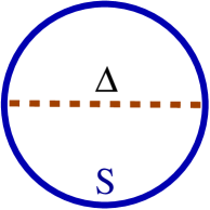
Figure 1: The two-loop diagram corresponding to the Yukawa interaction (20) contributing to the 2PI effective action (21).

We shall work in the model of chiral fermions $\psi_{L,R}$ (1), which couple via Yukawa interactions to scalars $\phi$,

$${\cal L}_{\rm int} = -\bar{\psi}_{L}y\phi\psi_{R}-\bar{\psi}_{R}(y\phi)^{\dagger}\psi_{L}$$ (20)

$$= -\bar{\psi}\left(P_{R}\otimes y\phi+P_{L}\otimes(y\phi)^{\dagger}\right)\psi\,,$$

where $P_{L,R}=(1\mp\gamma^{5})/2$ denote the chiral projectors, $y$ is the Yukawa coupling, which is a matrix (vector) in the scalar (fermionic) flavor space, and $\otimes$ denotes a direct product of the spinor and flavor spaces. Provided the momenta are not too small, the dynamics of fermions and scalars at the electroweak scale is expected to be perturbative, and the simplest nontrivial contribution to the effective action $\Gamma_{2}$ in (LABEL:2PI_effective_action) from the two-particle irreducible vacuum graphs arises from the two-loop diagram shown in figure 1. A perturbative treatment is justified as long as we are interested in modelling the dynamics of nearly thermal quasiparticles, which are predominantly responsible for the sources and thermalisation processes discussed in this work, since a majority of quasiparticles carry nearly thermal momenta. After an easy calculation we find

$$\Gamma_{\rm 2}=-\int_{{\cal C}}d^{4}u\,d^{4}v\;{\rm Tr}\big{[}P_{R}\otimes y^{l}S(u,v)P_{L}\otimes{y^{l^{\prime}}}^{\dagger}S(v,u)\big{]}\,\Delta_{ll^{\prime}}(u,v)\,,$$ (21)

from which we get the following one-loop expressions for the self-energies:

$$\Pi^{ac}_{ll^{\prime}}(u,v) = \;\;\,iac\frac{\delta\Gamma_{2}[\Delta,S]}{\delta\Delta^{ca}_{l^{\prime}l}(v,u)}$$ (22)

$$= -i{\rm Tr}\,\big{[}P_{R}\otimes y^{l^{\prime}}S^{ca}(v,u)P_{L}\otimes{y^{l}}^{\dagger}S^{ac}(u,v)\big{]}$$

$$\Sigma^{ac}(u,v) = -iac\frac{\delta\Gamma_{2}[\Delta,S]}{\delta S^{ca}(v,u)}$$ (23)

$$= i\big{[}P_{L}\otimes{y^{l}}^{\dagger}S^{ac}(u,v)P_{R}\otimes y^{l^{\prime}}\Delta_{l^{\prime}l}^{ca}(v,u)+P_{R}\otimes y^{l}S^{ac}(u,v)P_{L}\otimes{y^{l^{\prime}}}^{\dagger}\Delta_{ll^{\prime}}^{ac}(u,v)\big{]}\,.$$

The indices $l$ and $l^{\prime}$ denote scalar flavor. For the treatment of the collision term we need the self-energies

$$\Pi^{<,>}(u,v) \equiv \Pi^{+-,-+}(u,v)=-i{\rm Tr}\,\big{[}P_{R}\otimes yS^{>,<}(v,u)P_{L}\otimes y^{\dagger}S^{<,>}(u,v)\big{]}$$ (24)

$$\Sigma^{<,>}(u,v) \equiv \Sigma^{+-,-+}(u,v)=i\big{[}P_{L}\otimes y^{\dagger}S^{<,>}(u,v)P_{R}\otimes y\Delta^{>,<}(v,u)$$

$$\hphantom{XXXXXXXXX}+P_{R}\otimes yS^{<,>}(u,v)P_{L}\otimes y^{\dagger}\Delta^{<,>}(u,v)\big{]}\,.$$

Equations (2-3) together with (22-23) represent a closed set of equations for the quantum dynamics of scalar and fermionic fields described by the Lagrangean (1). This description is accurate in the weak coupling limit, in which the Yukawa couplings satisfy $\|y\|\ll 1$. One can in fact study the quantum dynamics of scalar fields also in the strongly coupled regime by making use of the 1/N expansion, where N denotes the number of scalar field components Berges:2002 ; BergesSerreau:2002 ; AartsAhrensmeierBaierBergesSerreau:2002 . Rather than studying this rather general problem, we proceed to develop approximations which are appropriate in the presence of slowly varying scalar field condensates close to thermal equilibrium. In this case a gradient expansion can be applied to simplify the problem.

By making use of (LABEL:Gtt_by_G<>) it is easy to show that the self-energies $\Pi^{t}$ and $\Pi^{\bar{t}}$ satisfy (LABEL:Pit-Pi<>) with $\Pi^{\tt sg}=0$, representing a nontrivial consistency check of our loop approximation scheme for the self-energies. Of course this check works as well for the fermionic self-energies.

2.1 Scalar collision term

We begin with the analysis of the collision term (4) of the scalar kinetic equation in the Wigner representation. We expand the diamond operator to first order in gradients and obtain two contributions, in the following referred to as zeroth and first order collision term, respectively (although the “zeroth order” contribution in fact is of first order in gradients, as we will see):

$${\cal C}_{\phi} = {\cal C}_{\phi 0}+{\cal C}_{\phi 1}$$ (26)

$$= -\frac{1}{2}\Big{(}i\Pi^{>}i\Delta^{<}-i\Pi^{<}i\Delta^{>}\Big{)}+\frac{i}{2}\diamond\Big{(}\left\{i\Pi^{>}\right\}\left\{i\Delta^{<}\right\}-\left\{i\Pi^{<}\right\}\left\{i\Delta^{>}\right\}\Big{)}\,.$$

We shall now consider the scalar collision term for a single scalar and fermionic field, and then generalise our analysis to the case of scalar and fermionic mixing in the next section.

2.1.1 The scalar collision term with no mixing

The one-loop expression for the single-field scalar self-energy (vacuum polarization) (24) in the Wigner representation reads

$$i\Pi^{<,>}(k,x)=-|y|^{2}\,\int\frac{d^{4}k^{\prime}d^{4}k^{\prime\prime}}{(2\pi)^{8}}(2\pi)^{4}\delta^{4}(k+k^{\prime}-k^{\prime\prime}){\rm Tr}\,\big{[}P_{R}iS^{>,<}(k^{\prime},x)P_{L}iS^{<,>}(k^{\prime\prime},x)\big{]}\,,$$ (27)

where $P_{L,R}=(\mathbbm{1}\mp\gamma^{5})/2$ are the projectors on left- and right-handed chirality states. A graphical representation of this one-loop self-energy is shown in figure 2. The hermiticity property (LABEL:S_herm_config) of the fermionic Wigner function immediately implies the hermiticity relation

$$\big{(}i\Pi^{<,>}(k,x)\big{)}^{\dagger}=i\Pi^{<,>}(k,x)\,,$$ (28)

which holds in general for reasonable truncations of the scalar self-energy.

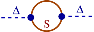
Figure 2: The one-loop scalar vacuum polarization diagram (27) from the Yukawa interaction (20), which contributes to the collision term of the scalar kinetic equation (2).

With the above expression for the self-energy we can write the zeroth order collision term in (26) as

$${\cal C}_{\phi 0} = \frac{|y|^{2}}{2}\,\int\frac{d^{4}k^{\prime}d^{4}k^{\prime\prime}}{(2\pi)^{8}}(2\pi)^{4}\delta^{4}(k+k^{\prime}-k^{\prime\prime})$$ (29)

$$\times \Big{\{}{\rm Tr}\,\big{[}P_{R}iS^{<}(k^{\prime})P_{L}iS^{>}(k^{\prime\prime})\big{]}i\Delta^{<}(k)-{\rm Tr}\,\big{[}P_{R}iS^{>}(k^{\prime})P_{L}iS^{<}(k^{\prime\prime})\big{]}i\Delta^{>}(k)\Big{\}},$$

where we suppressed the (local) $x$-coordinate dependence for notational simplicity. We insert the spin-diagonal decomposition (11) of the fermionic Wigner function and take the trace. Because of the chiral projectors within the trace, the component functions $g_{1}^{s}$ and $g_{2}^{s}$ do not contribute. With the help of the relation

$${\rm Tr}\,\Big{[}P_{R}P_{s^{\prime}}(k^{\prime})P_{s^{\prime\prime}}(k^{\prime\prime})\Big{]}=\frac{1}{2}\Bigg{(}1+s^{\prime}s^{\prime\prime}\frac{k_{0}^{\prime}k_{0}^{\prime\prime}-\vec{k}_{\|}^{\prime}\cdot\vec{k}_{\|}^{\prime\prime}}{\tilde{k_{0}^{\prime}}\tilde{k_{0}^{\prime\prime}}}\Bigg{)}.$$ (30)

we then find

$${\cal C}_{\phi 0} = \frac{|y|^{2}}{4}\,\sum_{s^{\prime}s^{\prime\prime}}\int\frac{d^{4}k^{\prime}d^{4}k^{\prime\prime}}{(2\pi)^{8}}(2\pi)^{4}\delta^{4}(k+k^{\prime}-k^{\prime\prime})s^{\prime}s^{\prime\prime}\Bigg{(}1+s^{\prime}s^{\prime\prime}\frac{k_{0}^{\prime}k_{0}^{\prime\prime}-\vec{k}_{\|}^{\prime}\cdot\vec{k}_{\|}^{\prime\prime}}{\tilde{k_{0}^{\prime}}\tilde{k_{0}^{\prime\prime}}}\Bigg{)}$$ (31)

$$\times\,\Big{\{}\Big{(}g_{0}^{s^{\prime}<}(k^{\prime})-g_{3}^{s^{\prime}<}(k^{\prime})\Big{)}\Big{(}g_{0}^{s^{\prime\prime}>}(k^{\prime\prime})+g_{3}^{s^{\prime\prime}>}(k^{\prime\prime})\Big{)}i\Delta^{<}(k)$$

$$\hphantom{X}-\Big{(}g_{0}^{s^{\prime}>}(k^{\prime})-g_{3}^{s^{\prime}>}(k^{\prime})\Big{)}\Big{(}g_{0}^{s^{\prime\prime}<}(k^{\prime\prime})+g_{3}^{s^{\prime\prime}<}(k^{\prime\prime})\Big{)}i\Delta^{>}(k)\Big{\}}\,.$$

In our tree-level analysis of fermions in section LABEL:Kinetics_of_fermions:_tree-level_analysis we found relations that enabled us to express all fermionic component functions in terms of $g^{s}_{0}$. Here we need only equation (LABEL:ced:diag3b) for $g^{s}_{3}$, which for one fermionic particle reduces to

$$g_{3}^{s<,>}=\frac{1}{\tilde{k}_{0}}\Big{[}sk_{z}\,g_{0}^{s<,>}+\frac{1}{2\tilde{k}_{0}}|m|^{2}\theta^{\prime}\partial_{k_{z}}g_{0}^{s<,>}+\frac{1}{2}{\cal C}_{\psi s3}\Big{]}\,.$$ (32)

In the following we neglect the collisional contribution in this relation, since it would result in terms which are of higher order in the coupling constant. We explained in the beginning of this section that the CP-violating sources, which contribute at first order in gradients to the collision term, are obtained by replacing the distribution functions in the on-shell Ansatz of the Wigner functions by the respective thermal distributions. For the remaining component $g^{s}_{0}$ of the fermionic Wigner function we therefore use

$$g_{0\,\rm eq}^{s<} = \hphantom{-}2\pi\delta\Big{(}k^{2}-|m|^{2}+\frac{1}{\tilde{k}_{0}}s|m|^{2}\theta^{\prime}\Big{)}|\tilde{k}_{0}|n_{\rm eq}(\hat{k}_{0})$$

$$g_{0\,\rm eq}^{s>} = -2\pi\delta\Big{(}k^{2}-|m|^{2}+\frac{1}{\tilde{k}_{0}}s|m|^{2}\theta^{\prime}\Big{)}|\tilde{k}_{0}|(1-n_{\rm eq}(\hat{k}_{0}))\,,$$ (33)

with the Fermi-Dirac distribution

$$n_{\rm eq}(\hat{k}_{0})=\frac{1}{e^{\beta\hat{k}_{0}}+1}$$ (34)

instead of the full distribution function. Note that we are working in the wall frame, which moves with the velocity $v_{w}$ within the rest frame of the plasma. Boosting the fermionic equilibrium Wigner function from the plasma frame to the wall frame results in the appearance of

$$\hat{k}_{0}\equiv\gamma_{w}(k_{0}+v_{w}k_{z})$$ (35)

in the argument of the equilibrium distribution. The CP-violating first order effects in the fermionic Wigner functions that have the potential to create collisional sources are the derivative term in the relation (32) between $g^{s}_{3}$ and $g^{s}_{0}$ and the energy shift in (33). Since in the scalar Wigner function there is no first order correction other than the non-thermal distribution, we can here simply use the equilibrium form

$$i\Delta_{\rm eq}^{<}(k) = 2\pi\delta(k^{2}-M^{2}){\rm sign}(k_{0})n^{\phi}_{\rm eq}(\hat{k}_{0})$$ (36)

$$i\Delta_{\rm eq}^{>}(k) = 2\pi\delta(k^{2}-M^{2}){\rm sign}(k_{0})(1+n^{\phi}_{\rm eq}(\hat{k}_{0}))\,,$$ (37)

again with the Bose-Einstein distribution

$$n^{\phi}_{\rm eq}(\hat{k}_{0})=\frac{1}{{\rm e}^{\beta\hat{k}_{0}}-1}$$ (38)

evaluated at $\hat{k}_{0}$. All terms in (31) without derivatives acting on $g^{s}_{0\,\rm eq}$ then drop out because of the KMS relations (cf. section LABEL:Equilibrium_Green_functions)

$$\Delta^{>}_{\rm eq} = {\rm e}^{\beta\hat{k}_{0}}\Delta^{<}_{\rm eq}$$

$$g_{0\,\rm eq}^{s>} = -e^{\beta\hat{k}_{0}}g_{0\,\rm eq}^{s<}$$ (39)

and the energy conserving delta function:

$${\cal C}_{\phi 0} = \frac{|y|^{2}}{8}|m|^{2}\theta^{\prime}\,\sum_{s^{\prime}s^{\prime\prime}}\int\frac{d^{4}k^{\prime}d^{4}k^{\prime\prime}}{(2\pi)^{8}}(2\pi)^{4}\delta^{4}(k+k^{\prime}-k^{\prime\prime})\Bigg{(}s^{\prime}s^{\prime\prime}+\frac{k_{0}^{\prime}k_{0}^{\prime\prime}-\vec{k}_{\|}^{\prime}\cdot\vec{k}_{\|}^{\prime\prime}}{\tilde{k_{0}^{\prime}}\tilde{k_{0}^{\prime\prime}}}\Bigg{)}$$

$$\times \Bigg{\{}\bigg{[}\frac{1}{\tilde{k_{0}^{\prime}}^{2}}\partial_{k_{z}^{\prime}}g_{0\,\rm eq}^{s^{\prime}<}(k^{\prime})\Big{(}1-\frac{s^{\prime\prime}k_{z}^{\prime\prime}}{\tilde{k_{0}^{\prime\prime}}}\Big{)}g_{0\,\rm eq}^{s^{\prime\prime}>}(k^{\prime\prime})-\Big{(}1+\frac{s^{\prime}k_{z}^{\prime}}{\tilde{k_{0}^{\prime}}}\Big{)}g_{0\,\rm eq}^{s^{\prime}<}(k^{\prime})\frac{1}{\tilde{k_{0}^{\prime\prime}}^{2}}\partial_{k_{z}^{\prime\prime}}g_{0\,\rm eq}^{s^{\prime\prime}>}(k^{\prime\prime})\bigg{]}i\Delta^{<}_{\rm eq}(k)$$

$$\hphantom{i}-\bigg{[}\frac{1}{\tilde{k_{0}^{\prime}}^{2}}\partial_{k_{z}^{\prime}}g_{0\,\rm eq}^{s^{\prime}>}(k^{\prime})\Big{(}1-\frac{s^{\prime\prime}k_{z}^{\prime\prime}}{\tilde{k_{0}^{\prime\prime}}}\Big{)}g_{0\,\rm eq}^{s^{\prime\prime}<}(k^{\prime\prime})-\Big{(}1+\frac{s^{\prime}k_{z}^{\prime}}{\tilde{k_{0}^{\prime}}}\Big{)}g_{0\,\rm eq}^{s^{\prime}>}(k^{\prime})\frac{1}{\tilde{k_{0}^{\prime\prime}}^{2}}\partial_{k_{z}^{\prime\prime}}g_{0\,\rm eq}^{s^{\prime\prime}<}(k^{\prime\prime})\bigg{]}i\Delta^{>}_{\rm eq}(k)\Bigg{\}}\,.\qquad$$

This expression for the scalar collision term is already explicitly of first order in gradients, so we can neglect the spin-dependent shift in the spectral delta functions in (33). The resulting spin-independent function, living on the unperturbed mass shell $\delta(k^{2}-|m|^{2})$, is denoted by $g_{0\,\rm eq}$. We can now sum over spins and, taking into account correction terms caused by the momentum derivatives

$$\partial_{k_{z}}g_{0\,\rm eq}^{s>}(k)=-e^{\beta\hat{k}_{0}}\left(\partial_{k_{z}}g_{0\,\rm eq}^{s<}+\beta\gamma_{w}v_{w}g_{0\,\rm eq}^{s<}\right)\,,$$ (41)

use the KMS relation for the remaining terms to obtain

$${\cal C}_{\phi 0} = -\frac{|y|^{2}}{2}\beta\gamma_{w}v_{w}|m|^{2}\theta^{\prime}\int\frac{d^{4}k^{\prime}d^{4}k^{\prime\prime}}{(2\pi)^{8}}(2\pi)^{4}\delta^{4}(k+k^{\prime}-k^{\prime\prime})$$ (42)

$$\times \frac{k_{0}^{\prime}k_{0}^{\prime\prime}-\vec{k}_{\|}^{\prime}\cdot\vec{k}_{\|}^{\prime\prime}}{\tilde{k_{0}^{\prime}}\tilde{k_{0}^{\prime\prime}}}g^{<}_{0\,\rm eq}(k^{\prime})g^{>}_{0\,\rm eq}(k^{\prime\prime})i\Delta^{<}_{\rm eq}(k)\bigg{(}\frac{1}{({\tilde{k}_{0}^{\prime}})^{2}}+\frac{1}{({\tilde{k}_{0}^{\prime\prime}})^{2}}\bigg{)}\,.$$

This collisional source is proportional to the wall velocity $v_{w}$. This displays the fact that for a wall at rest the leading order Wigner functions indeed form an equilibrium solution.

At linear order in $v_{w}$ the equilibrium relation

$$g_{0\,\rm eq}^{<,>}(-k_{0}^{\prime})=-g_{0\,\rm eq}^{>,<}(k_{0}^{\prime})$$ (43)

allows one to make the replacement $k^{\prime}\leftrightarrow-k^{\prime\prime}$ in the last term within brackets, so that Eq. (42) can be rewritten as

$${\cal C}_{\phi 0}(k) = -|y|^{2}\frac{v_{w}|m|^{2}\theta^{\prime}}{T}\,i\Delta^{<}_{\rm eq}(k){\cal I}^{>}_{\phi 0}(k)$$ (44)

$${\cal I}^{<,>}_{\phi 0}(k) = \int\frac{d^{4}k^{\prime}d^{4}k^{\prime\prime}}{(2\pi)^{4}}\delta^{4}(k+k^{\prime}-k^{\prime\prime})\frac{1}{(\tilde{k_{0}^{\prime}})^{2}}\frac{k_{0}^{\prime}k_{0}^{\prime\prime}-\vec{k}_{\|}^{\prime}\cdot\vec{k}_{\|}^{\prime\prime}}{\tilde{k_{0}^{\prime}}\tilde{k_{0}^{\prime\prime}}}g_{0\,\rm eq}^{>,<}(k^{\prime})g_{0\,\rm eq}^{<,>}(k^{\prime\prime})\,.$$ (45)

Recall also that as a consequence of the KMS condition ${\cal I}^{>}_{\phi 0}(k)i\Delta^{<}(k)={\cal I}^{<}_{\phi 0}(k)i\Delta^{>}(k)$. In Appendix A we show how, by performing all but one of the integrations in (45), ${\cal I}_{\phi 0}\equiv{\cal I}_{\phi 0}^{>}$ can be reduced to a single integral (157), such that the scalar collisional source simplifies to

$${\cal C}_{\phi 0} = -|y|^{2}\frac{v_{w}|m|^{2}\theta^{\prime}}{8T}\,\frac{\theta(M-2|m|)}{\omega_{\phi}}\int_{0}^{\infty}\frac{dk^{\prime}}{\omega_{0}^{\prime}}\theta(k^{2}{k^{\prime}}^{2}-\beta_{0}^{2})\Big{[}\theta(k_{0})\delta(k_{0}-\omega_{\phi})+\theta(-k_{0})\delta(k_{0}+\omega_{\phi})\Big{]}$$ (46)

$$\times \Big{[}\frac{M^{2}}{2|m|}\Re\frac{1}{\sqrt{(k_{z}-c_{-})(c_{+}-k_{z})}}+\Im\frac{k_{z}}{\sqrt{(k_{z}-c_{-})(c_{+}-k_{z})}}-\frac{k^{\prime}}{k}\Big{]}$$

$$\times f^{\phi}_{0}(1-\bar{f}_{0}^{\prime})\Big{[}\theta(\omega_{0}^{\prime\prime})f_{0}^{\prime\prime}|_{\omega_{0}^{\prime\prime}=\omega_{0}^{\prime}-\omega_{\phi}}-\theta(\omega_{0}^{\prime\prime})(1-f_{0}^{\prime\prime})|_{\omega_{0}^{\prime\prime}=\omega_{\phi}-\omega_{0}^{\prime}}\Big{]}\,.$$

The $c_{\pm}$ and $\beta_{0}$ are defined in Eqs. (156) and (151) in Appendix A, and

$$f^{\phi}_{0}\equiv n_{\rm eq}^{\phi}(\omega_{\phi})=\frac{1}{{\rm e}^{\beta\omega_{\phi}}-1}\,,\quad f_{0}=\bar{f}_{0}\equiv n_{\rm eq}(\omega_{0})=\frac{1}{{\rm e}^{\beta\omega_{0}}+1}\,.$$ (47)

Note that the source contains a mass threshold: it is nonzero only if

$$M>2|m|\,.$$ (48)

The physical reason for this threshold is that in the one loop self-energy only on-shell absorption and emission processes are allowed. Together with the energy-momentum conservation, this leads to the above condition.

We now make a slight digression and consider the first order collision term in (26). Because of the derivative in the diamond operator this term is already of first order in gradients and we can use the leading order equilibrium Wigner functions for its computation. Then the KMS relations (39) induce a similar relation for the scalar self-energy,

$$\Pi_{\rm eq}^{>}(k)={\rm e}^{\beta\hat{k}_{0}}\Pi_{\rm eq}^{<}(k)\,,$$ (49)

and we find

$${\cal C}_{\phi 1} = -\frac{1}{4}\Big{(}\partial_{k_{z}}\beta\hat{k}_{0}\Big{)}\partial_{z}\Big{(}\Pi^{>}_{\rm eq}(k)i\Delta^{<}_{\rm eq}(k)\Big{)}$$ (50)

$$= \frac{|y|^{2}}{4}\beta\gamma_{w}v_{w}\partial_{z}\int\frac{d^{4}k^{\prime}d^{4}k^{\prime\prime}}{(2\pi)^{8}}(2\pi)^{4}\delta(k+k^{\prime}-k^{\prime\prime}){\rm Tr}[P_{R}S_{\rm eq}^{<}(k^{\prime})P_{L}S_{\rm eq}^{>}(k^{\prime\prime})]i\Delta_{\rm eq}^{<}(k)\,.$$

Following a similar procedure as in the leading order term, this can be reduced to

$${\cal C}_{\phi 1}=-i\frac{|y|^{2}}{2}\beta\gamma_{w}v_{w}\partial_{z}\int\frac{d^{4}k^{\prime}d^{4}k^{\prime\prime}}{(2\pi)^{8}}(2\pi)^{4}\delta(k+k^{\prime}-k^{\prime\prime})\frac{k_{0}^{\prime}k_{0}^{\prime\prime}-\vec{k}^{\prime}\cdot\vec{k}^{\prime\prime}}{\tilde{k_{0}^{\prime}}\tilde{k_{0}^{\prime\prime}}}g_{0\,\rm eq}^{<}(k^{\prime})g_{0\,\rm eq}^{>}(k^{\prime\prime})i\Delta^{<}_{\rm eq}(k)\,.$$ (51)

It is now clear from Eqs. (9) and (LABEL:scalar_pos_freq_deltaCP) that this first order term contributes only to the constraint equation, since $({\cal C}_{\phi 1})^{\dagger}=-{\cal C}_{\phi 1}$ is antihermitean. Furthermore, one can show that this contribution to the constraint equation results in a subdominant contribution in the kinetic equation, and hence can be consistently neglected.

In anticipation of the discussion of fluid equations in section 4 we remark that the CP-violating sources in the fluid equations are obtained by taking moments of the scalar kinetic equation (9) for the CP-violating distribution function. We note that the zeroth order collisional source ${\cal C}_{\phi 0}$ (42) is real and symmetric in the momentum argument:

$${\cal C}_{\phi 0}^{\dagger}={\cal C}_{\phi 0}^{*}={\cal C}_{\phi 0}\,,\qquad{\cal C}_{\phi 0}(-k,x)={\cal C}_{\phi 0}(k,x)\,.$$ (52)

The symmetry is a simple consequence of the relation

$$\delta(k_{0}+k_{0}^{\prime}-k_{0}^{\prime\prime})g_{0\,\rm eq}^{>}(k_{0}^{\prime})g_{0\,\rm eq}^{<}(k_{0}^{\prime\prime})\;\rightarrow\;\delta(-k_{0}+k_{0}^{\prime}-k_{0}^{\prime\prime})g_{0\,\rm eq}^{<}(k_{0}^{\prime\prime})g_{0\,\rm eq}^{>}(k_{0}^{\prime}),$$ (53)

where we made use of Eq. (43). We furthermore recall that the first order source (51) is antihermitean, such that the following relation holds:

$$\frac{1}{2}\big{[}{\cal C}_{\phi}(k,x)+{\cal C}^{\dagger}_{\phi}(k,x)+{\cal C}^{*}_{\phi}(-k,x)+{\cal C}^{T}_{\phi}(-k,x)\big{]}=2{\cal C}_{\phi 0}(k,x)\,.$$ (54)

From Eq. (147) and (150) it follows that the integrand function in the scalar collisional source ${\cal C}_{\phi}={\cal C}_{\phi 0}$ is of the form $\int dk_{z}^{\prime}F(k_{z}k_{z}^{\prime},k_{z}^{2},{k_{z}^{\prime}}^{2})$, so that simple changes of variables imply

$$\int_{-\infty}^{0}dk_{z}\int dk_{z}^{\prime}F(k_{z}k_{z}^{\prime},k_{z}^{2},{k_{z}^{\prime}}^{2}) = \;\;\;\int_{0}^{\infty}dk_{z}\int dk_{z}^{\prime}F(k_{z}k_{z}^{\prime},k_{z}^{2},{k_{z}^{\prime}}^{2})$$

$$\int_{-\infty}^{0}dk_{z}\,k_{z}\,\int dk_{z}^{\prime}F(k_{z}k_{z}^{\prime},k_{z}^{2},{k_{z}^{\prime}}^{2}) = -\int_{0}^{\infty}dk_{z}\,k_{z}\,\int dk_{z}^{\prime}F(k_{z}k_{z}^{\prime},k_{z}^{2},{k_{z}^{\prime}}^{2})\,,$$ (55)

and we immediately conclude that the source in the scalar Euler fluid equation, which is obtained by taking the first moment of Eq. (9), vanishes:

$$\int\frac{d^{4}k}{4\pi^{4}}\theta(k_{0})\frac{k_{z}}{\omega_{\phi}}{\cal C}_{\phi}=0\,.$$ (56)

The same conclusion is reached upon observing that ${\cal C}_{\phi}$ is symmetric under $k_{z}\rightarrow-k_{z}$.

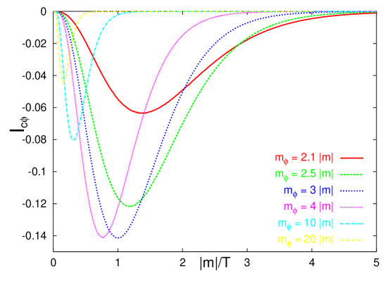
Figure 3: The integral in the CP-violating collisional source (57) of the scalar continuity fluid equation as a function of the mass parameters, $M/T$ and $|m|/T$.

The source in the continuity equation, which is the 0th moment of (9), does not vanish, however. Indeed, upon performing the $k_{0}$, $k_{z}$ and angular (azimuthal) integrations in (46), we obtain

$${\cal S}_{\phi}^{\rm coll} \equiv 2\int\frac{d^{4}k}{(2\pi)^{4}}{\cal C}_{\phi 0}=-\frac{|y|^{2}}{8\pi^{3}}v_{w}(|m|^{2}\theta^{\prime})\,T\,\theta(M-2|m|)\;{\cal I}_{c\phi}$$

$${\cal I}_{c\phi} = \beta^{2}\int_{0}^{\infty}\frac{kdk}{\omega_{\phi}}\int_{0}^{\infty}\frac{dk^{\prime}}{\omega_{0}^{\prime}}\theta(k^{2}{k^{\prime}}^{2}-\beta_{0}^{2})$$ (57)

$$\times \bigg{[}\frac{M^{2}}{2|m|}\arctan\Big{(}\frac{k^{\prime}}{|m|}\Big{)}-\frac{\beta_{0}}{k^{\prime}}\bigg{(}1-\frac{|m|}{k^{\prime}}\arctan\Big{(}\frac{k^{\prime}}{|m|}\Big{)}\bigg{)}-k^{\prime}\bigg{]}$$

$$\times f^{\phi}_{0}(1-\bar{f}_{0}^{\prime})\Big{[}\theta(\omega_{0}^{\prime\prime})(1-f_{0}^{\prime\prime})|_{\omega_{0}^{\prime\prime}=\omega_{0}^{\prime}-\omega_{\phi}}-\theta(\omega_{0}^{\prime\prime})(1-f_{0}^{\prime\prime})|_{\omega_{0}^{\prime\prime}=\omega_{\phi}-\omega_{0}^{\prime}}\Big{]}\,.$$

We now evaluate this collisional source numerically as a function of the mass parameters, $M/T$ and $|m|/T$ ($M\geq 2|m|$). The result is shown in figure 3. The source peaks at $|m|\approx 1T$ and $M\approx(3-4)T$, and it is (exponentially) Boltzmann suppressed when $|m|,M\gg T$. Note that the nature of the collisional source (57) is quite different from the source (LABEL:boltzmann:deltaf-a_source) arising from the semiclassical force in the flow term. In particular, the source (57) is a consequence of CP-violation in the fermionic Wigner function, which circles in the one-loop self-energy shown in figure 2, and it is hence suppressed by the Yukawa coupling squared, $|y|^{2}$. Moreover, the source exhibits a kinematic mass threshold, $M\geq 2|m|$, which is a consequence of the on-shell approximation in the fermionic Wigner functions. The threshold is of course absent in the semiclassical force source. To get a rough estimate of how strong the source can be, we take $v_{w}\sim 0.03$, $|m|\sim T$, $M\sim 3T$, $|y|\sim 1$, $\theta^{\prime}\sim 0.1T$ (maximum CP-violation), such that ${\cal S}_{\phi}^{\rm coll}\sim 10^{-6}T^{4}$.

2.1.2 The scalar collision term with mixing

We shall now study the scalar collision term in the case of scalar and fermionic mixing, for which the Lagrangean (20) reads

$${\cal L}^{\prime}_{\rm Yu}=-\phi^{l}\bar{\psi}_{L}y^{l}\psi_{R}+{\rm h.c.}\,=-\bar{\psi}\left(P_{R}\otimes\phi^{l}y^{l}+P_{L}\otimes{\phi^{l}}^{*}{y^{l}}^{\dagger}\right)\psi\,,$$ (58)

where $y^{l}=(y^{l}_{ij})$ is a matrix in the fermionic flavor space and $l$ denotes the different scalar particles. The one-loop scalar self-energy is a straightforward generalization of (27),

$$i\Pi^{<,>}_{ll^{\prime}}(k,x) = -\int\frac{d^{4}k^{\prime}d^{4}k^{\prime\prime}}{(2\pi)^{8}}(2\pi)^{4}\delta^{4}(k+k^{\prime}-k^{\prime\prime}){\rm Tr}\Big{(}P_{R}\otimes y^{l}iS^{>,<}(k^{\prime},x)P_{L}\otimes y^{l^{\prime}\dagger}iS^{<,>}(k^{\prime\prime},x)\Big{)},\qquad$$ (59)

where the trace is now to be taken both in spinor and in fermionic flavor space. The mixing in the bosonic sector was handled in the flow term by a unitary rotation into the basis in which the mass is diagonal (cf. section LABEL:Kinetics_of_scalars:_tree-level_analysis), resulting in Eq. (9), so that an identical rotation has to be performed also in the collision term (26).

Let us consider first the influence of the scalar mixing. The scalar collision term is now to be understood as a product of two matrices in the scalar flavor space. After the rotation into the diagonal basis the form is maintained. The self-energy gets rotated as $i\Pi^{<,>}\rightarrow i\Pi^{<,>}_{d}=Ui\Pi^{<,>}U^{\dagger}$, which corresponds to the following redefinition of the couplings, $y\rightarrow y_{d}=Uy$ and $y^{\dagger}\rightarrow{y}^{\,\dagger}_{d}=y^{\dagger}U^{\dagger}$ in (59). The diagonal contributions to the zeroth order collision term contain the terms $y_{d}^{l}{y_{d}^{l^{\prime}}}^{\,\dagger}\,i\Delta^{<,>}_{d,l^{\prime}l}$, such that the off-diagonals $(1-\delta_{ll^{\prime}})i\Delta^{<,>}_{d,l^{\prime}l}$ may give rise to a CP-violating contribution when either the Yukawa couplings $y_{d}^{l}$ or $i\Delta^{<,>}_{d,l^{\prime}l}$ are CP-violating. Treating the latter contributions properly would require the dynamical treatment of the off-diagonals, which is beyond the scope of this work. Note that there is no contribution at order $\hbar$ coming from the diagonals of $i\Delta^{<,>}_{d}$. For a diagrammatic illustration of the problem see figure 4 below. The diagonal elements of the first order collision term are imaginary, and therefore do not contribute to the kinetic equation.

Next, we consider the question of fermionic mixing (cf. section LABEL:Flavor_diagonalization). In this case the mass $m$ in the free part of the fermionic Lagrangean (1) is a non-hermitean matrix in flavor space. The diagonal basis is defined by

$$m_{d}\equiv UmV^{\dagger}={\rm diag}\Big{[}|m_{j}|{\rm e}^{i\theta_{j}}\Big{]},$$ (60)

where $U$ and $V$ are the unitary matrices that diagonalize $m$. Since the self-energy (59) is a trace in the fermionic flavor space, its form stays invariant and we just have to replace the fermionic Wigner function and the coupling matrix by the rotated versions. For notational simplicity we shall work with only one scalar particle, and drop the superfluous indices $d$. The fermionic Wigner function may contain both diagonal and off-diagonal elements in the flavor diagonal basis.

Let us first consider the contribution from the diagonal elements. To this purpose we write the fermionic Wigner functions as $S^{<,>}_{ij}\rightarrow\delta_{ij}S^{<,>}_{i}+{\cal O}(\hbar)$, so that we have:

$$i\Pi^{<,>}(k,x)=\sum_{ij}y_{ij}y^{*}_{ij}\int\frac{d^{4}k^{\prime}d^{4}k^{\prime\prime}}{(2\pi)^{8}}(2\pi)^{4}\delta^{4}(k+k^{\prime}-k^{\prime\prime})\\ {\rm Tr}\Big{(}P_{R}S^{>,<}_{j}(k^{\prime},x)P_{L}S_{i}^{<,>}(k^{\prime\prime},x)\Big{)}.$$

The trace is now to be taken in the spinor space only. We can go through the same steps as in the non-mixing case of section 2.1.1, always keeping track of the indices attached to the fermionic functions. One difference in comparison to the non-mixing case is that in relation (LABEL:ced:diag3b) between $g^{s}_{3}$ and $g^{s}_{0}$ there is an additional term from the fermionic flavor rotation. The expression analogous to (42) is then

$${\cal C}_{\phi 0}(k,x) = -\frac{1}{2}\beta v_{w}\int\frac{d^{4}k^{\prime}d^{4}k^{\prime\prime}}{(2\pi)^{8}}(2\pi)^{4}\delta^{4}(k+k^{\prime}-k^{\prime\prime})\frac{k^{\prime}_{0}k^{\prime\prime}_{0}-\vec{k}^{\prime}_{\|}\cdot\vec{k}^{\prime\prime}_{\|}}{\tilde{k}_{0}^{\prime}\tilde{k}_{0}^{\prime\prime}}$$

$$\times \sum_{ij}|y_{ij}|^{2}g^{>}_{0i\,\rm eq}(k^{\prime})g^{<}_{0j\,\rm eq}(k^{\prime\prime})i\Delta^{>}_{0\,\rm eq}(k)\left(\frac{\big{(}|m|^{2}(\theta^{\prime}+2\Delta_{z})\big{)}_{i}}{\tilde{k}_{0}^{\prime 2}}+\frac{\big{(}|m|^{2}(\theta^{\prime}+2\Delta_{z})\big{)}_{j}}{\tilde{k}_{0}^{\prime\prime 2}}\right),$$

where $\Delta_{z}=\frac{i}{2}(V\partial_{z}V^{\dagger}-U\partial_{z}U^{\dagger})$. Upon performing a similar change of variables as in the non-mixing case, $k_{0}^{\prime}\leftrightarrow-k_{0}^{\prime\prime}$ and $i\leftrightarrow j$, we have

$$\delta^{4}(k_{0}+k_{0}^{\prime}-k_{0}^{\prime\prime})g_{0i\,\rm eq}^{s^{\prime}>}(k_{0}^{\prime})g_{0j\,\rm eq}^{s^{\prime\prime}<}(k_{0}^{\prime\prime})\;\rightarrow\;\delta^{4}(-k_{0}+k_{0}^{\prime}-k_{0}^{\prime\prime})g_{0j\,\rm eq}^{s^{\prime}<}(k_{0}^{\prime\prime})g_{0i\,\rm eq}^{s^{\prime\prime}>}(k_{0}^{\prime}),$$ (62)

such that Eq. (2.1.2) can be recast as

$${\cal C}_{\phi 0} = \sum_{ij}\frac{|y_{ij}|^{2}+|y_{ji}|^{2}}{2}\frac{v_{w}(|m|^{2}\theta^{\prime})_{i}}{T}\,{\cal I}^{>}_{\phi 0ij}(k)i\Delta^{<}_{\rm eq}(k)$$

$${\cal I}^{<,>}_{\phi 0ij}(k) = \int\frac{d^{4}k^{\prime}d^{4}k^{\prime\prime}}{(2\pi)^{8}}(2\pi)^{4}\delta(k+k^{\prime}-k^{\prime\prime})\frac{k_{0}^{\prime}k_{0}^{\prime\prime}-\vec{k}_{\|}^{\prime}\cdot\vec{k}_{\|}^{\prime\prime}}{\tilde{k_{0}^{\prime}}\tilde{k_{0}^{\prime\prime}}}g_{0i\,\rm eq}^{>,<}(k^{\prime})g_{0j\,\rm eq}^{<,>}(k^{\prime\prime})\frac{1}{(\tilde{k_{0}^{\prime}})^{2}}\,.$$ (63)

This integral can be evaluated in part; upon performing analogous steps as in the one field case, one arrives at the result

$${\cal I}_{\phi 0ij}(k) = -\frac{\theta(M-|m_{i}|-|m_{j}|)}{8\pi^{2}}\int k^{\prime}dk^{\prime}\theta(k^{2}{k^{\prime}}^{2}-\beta_{0}^{2})\int_{k^{\prime}_{z_{1}}}^{k^{\prime}_{z_{2}}}\frac{dk^{\prime}_{z}}{(\tilde{\omega}_{0i}^{\prime})^{2}}\frac{{k_{z}^{\prime}}^{2}+k_{z}k_{z}^{\prime}-\frac{M^{2}-|m_{i}|^{2}-|m_{j}|^{2}}{2}}{\Big{[}(k^{\prime}_{z_{2}}-k^{\prime}_{z})(k^{\prime}_{z}-k^{\prime}_{z_{1}})\Big{]}^{\frac{1}{2}}}$$ (64)

$$\times \Bigg{[}\theta(\omega_{0i}^{\prime}-\omega_{\phi})\left[\theta(-k_{0})f_{0i}^{\prime}(1-f_{0j}^{\prime\prime})+\theta(k_{0})(1-\bar{f}_{0i}^{\prime})\bar{f}_{0j}^{\prime\prime}\right]$$

$$-\theta(\omega_{\phi}-\omega_{0i}^{\prime})\left[\theta(-k_{0})f_{0i}^{\prime}\bar{f}_{0j}^{\prime\prime}+\theta(k_{0})(1-\bar{f}_{0i}^{\prime})(1-f_{0j}^{\prime\prime})\right]\Bigg{]}\,,$$

which, in the one field limit, reduces to Eq. (152). By making use of the integrals (153), the $k_{z}^{\prime}$-integral can be evaluated. The final $k^{\prime}$ and $k$ integrals have to be performed numerically, the results are very similar to the ones presented in figure 3.

Like in the non-mixing case the first order collision term is imaginary and therefore does not contribute to the collisional sources at order $\hbar$. The self-energy stays imaginary, and the derivative from the diamond operator acts on the self-energy as a whole and does not notice the rotation. Finally, we remark on the contributions from the off-diagonal elements of the Wigner functions, $(1-\delta_{ij})iS^{<,>}_{ij}$, which are suppressed by at least one power of $\hbar$. In the case when the fermionic interaction and flavor bases do not coincide, it is clear that the off-diagonal elements of $iS^{<,>}_{ij}$ could in principle contribute to a CP-violating source at order $\hbar$ in the bosonic collision term (26). A proper treatment of this problem would require a dynamical treatment of the off-diagonal elements of $iS^{<,>}_{ij}$ (in the flavor diagonal basis) and it is beyond the scope of this work.

2.1.3 Discussion of scalar collisional sources

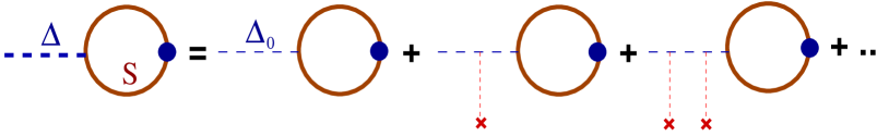
Figure 4: The one-loop collision term in the scalar kinetic equation in a theory with the Yukawa interaction (20). The interactions of the scalar propagator with the scalar condensate are of the same nature as the tree-level interactions discussed in section LABEL:Kinetics_of_scalars:_tree-level_analysis. Just like in the tree-level case, at order $\hbar$, scalars do not feel the condensate.

Contributions to the scalar CP-violating collisional source could, in principle, arise from the scalar or from the fermionic sector of the theory (1,20). In this section we have shown that, to order $\hbar$ in an expansion in gradients, there are no CP-violating contributions to the collision term of the scalar kinetic equation arising from the scalar sector. Our proof includes the more general case of mixing scalars. A simple qualitative argument in support of this is shown in figure 4.

On the other hand, as we have argued in sections 2.1.1 and 2.1.2, the fermionic contributions to the scalar one-loop self-energy do result in CP-violating effects which contribute to the collision term of the scalar kinetic equation. As illustrated in figure 5, these effects arise from CP-violating contributions to the fermionic propagators which run in the self-energy loop, and can be thought of as radiative contributions to the CP-violating scatterings off the Higgs condensate. These contributions can source CP-violating scalar currents in the Higgs or sfermionic sectors, for example, and thus may be of relevance for electroweak baryogenesis. From our one-loop study of the CP-violating source shown in figure 3 it follows that: (a) the source has a very different parametric dependence than the semiclassical source shown in figure LABEL:figure:flow-source, and (b) the source tends to be large in the case of fermions whose mass is of the order of the temperature, and where the scalar mass is a few times bigger. With $T\sim 100~{}{\rm GeV}$, popular extensions of the Standard Model, which include supersymmetric theories, typically contain such particles.

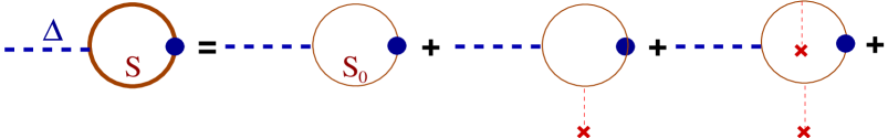
Figure 5: The collision term in the scalar kinetic equation as in figure 4. The interactions of the fermionic (loop) propagators with the scalar field condensate that can contribute in CP-odd manner at the order $\hbar$ to the scalar kinetic equation.

2.2 Fermionic collision term

Now we turn our attention to the collision term for fermions. Again, we expand in gradients, and distinguish between the zeroth and first order collision terms,

$${\cal C}_{\psi}={\cal C}_{\psi 0}+{\cal C}_{\psi 1}+..\,,$$ (65)

where

$${\cal C}_{\psi 0} = \frac{1}{2}\Big{(}\Sigma^{>}S^{<}-\Sigma^{<}S^{>}\Big{)}$$ (66)

$${\cal C}_{\psi 1} = -\frac{i}{2}\diamond\Big{(}\left\{\Sigma^{>}\right\}\left\{S^{<}\right\}-\left\{\Sigma^{<}\right\}\left\{S^{>}\right\}\Big{)}\,.$$ (67)

CP-violating contributions to the collision term appear, like in the scalar case, at first order in gradients. Since the calculational procedure of the sources is very similar to that in the scalar case, we shall outline only its main steps.

2.2.1 Fermionic collision term with no mixing

The single-field fermionic self-energy, when approximated by the one-loop expression (23) and written in Wigner space, reads

$$i\Sigma^{<,>} = |y|^{2}\int\frac{d^{4}k^{\prime}\,d^{4}k^{\prime\prime}}{(2\pi)^{4}}\,\delta^{4}(k-k^{\prime}+k^{\prime\prime})$$ (68)

$$\hskip 76.82234pt\times\;\big{[}i\Delta^{>,<}(k^{\prime\prime})P_{L}iS^{<,>}(k^{\prime})P_{R}+i\Delta^{<,>}(-k^{\prime\prime})P_{R}iS^{<,>}(k^{\prime})P_{L}\big{]}\,.$$

A graphical representation of this self-energy is shown in figure 6.

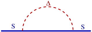
Figure 6: The one-loop fermionic vacuum polarization diagram (cf. Eq. (68)) from the Yukawa interaction (20), which contributes to the collision term (65) of the fermionic kinetic equation (3).

We again use the spin diagonal Ansatz (11) for the fermionic Wigner function, which in the self-energy shows up between two chiral projectors. This can be simplified by

$$P_{L}\sum_{s^{\prime}}S^{<,>}_{s^{\prime}}(k^{\prime})P_{R}=\sum_{s^{\prime}}iP_{s^{\prime}}(k^{\prime})s^{\prime}P_{L}\bigl{[}\gamma^{3}\gamma^{5}g^{s^{\prime}<,>}_{0}(k^{\prime})-\gamma^{3}g^{s^{\prime}<,>}_{3}(k^{\prime})\bigr{]}\,,$$ (69)

and similarly for $P_{L}\leftrightarrow P_{R}$, such that the self-energy becomes

$$i\Sigma^{<,>}(k)=-|y|^{2}\sum_{s^{\prime}}s^{\prime}\int\frac{d^{4}k^{\prime}\,d^{4}k^{\prime\prime}}{(2\pi)^{4}}\,\delta^{4}(k-k^{\prime}+k^{\prime\prime})P_{s^{\prime}}(k^{\prime})i\Delta^{>,<}(k^{\prime\prime})\left(\gamma^{3}\gamma^{5}g^{<,>s^{\prime}}_{0}(k^{\prime})-\gamma^{3}g^{<,>s^{\prime}}_{3}(k^{\prime})\right)\,.\quad\,$$ (70)

Again we use thermal distributions for the Wigner functions, and with

$$i\Delta^{<}_{\rm eq}(-k^{\prime\prime})=i\Delta^{>}_{\rm eq}(k^{\prime\prime})$$ (71)

the chiral projectors drop out of the zeroth order collision term:

$${\cal C}_{\psi 0} = \frac{|y|^{2}}{2}\sum_{s^{\prime}}\int\frac{d^{4}k^{\prime}d^{4}k^{\prime\prime}}{(2\pi)^{4}}\,\delta^{4}(k-k^{\prime}+k^{\prime\prime})\sum_{s,s^{\prime}}P_{s^{\prime}}(k^{\prime})P_{s}(k)s^{\prime}$$

$$\times\;\Big{[}i\Delta^{<}_{\rm eq}(k^{\prime\prime})\Big{(}\gamma^{3}\gamma^{5}g_{0\,\rm eq}^{s^{\prime}>}(k^{\prime})-\gamma^{3}g_{3\,\rm eq}^{s^{\prime}>}(k^{\prime})\Big{)}\Big{(}s\gamma^{3}\gamma^{5}g_{0\,\rm eq}^{s<}(k)-s\gamma^{3}g_{3\,\rm eq}^{s<}(k)+g_{1\,\rm eq}^{s<}(k)-i\gamma^{5}g_{2\,\rm eq}^{s<}(k)\Big{)}$$

$$-\,i\Delta^{>}_{\rm eq}(k^{\prime\prime})\Big{(}\gamma^{3}\gamma^{5}g_{0\,\rm eq}^{s^{\prime}<}(k^{\prime})-\gamma^{3}g_{3\,\rm eq}^{s^{\prime}<}(k^{\prime})\Big{)}\Big{(}s\gamma^{3}\gamma^{5}g_{0\,\rm eq}^{s>}(k)-s\gamma^{3}g_{3\,\rm eq}^{s>}(k)+g_{1\,\rm eq}^{s>}(k)-i\gamma^{5}g_{2\,\rm eq}^{s>}(k)\Big{)}\Big{]}\,.$$

It is not hard to see that, at leading order in gradients, the collision term vanishes.

The further procedure is now analogous to the scalar case. We use equations (LABEL:ced:diag1b-LABEL:ced:diag3b), simplified to the case of only one fermionic particle, to express the functions $g^{s}_{i\,\rm eq}$ ($i=1,2,3$) in terms of $g^{s}_{0\,\rm eq}$. The terms without derivatives acting on $g^{s}_{0\,\rm eq}$ vanish because of the KMS relations (39) and the energy-momentum conserving $\delta$-function, while Eq. (41) shows that all surviving terms are wall velocity suppressed - as they should be:

$${\cal C}_{\psi 0} = \frac{|y|^{2}}{4}\beta\gamma_{w}v_{w}\int\frac{d^{4}k^{\prime}d^{4}k^{\prime\prime}}{(2\pi)^{4}}\,\delta(k-k^{\prime}+k^{\prime\prime})\sum_{ss^{\prime}}P_{s^{\prime}}(k^{\prime})P_{s}(k)g_{0\,\rm eq}^{<}(k)g_{0\,\rm eq}^{>}(k^{\prime})i\Delta^{<}_{\rm eq}(k^{\prime\prime})$$ (73)

$$\hskip 99.58464pt\times\;\bigg{\{}\mathbbm{1}\bigg{[}|m|^{2}\theta^{\prime}\bigg{(}-s^{\prime}\frac{k_{z}}{\tilde{k}_{0}}\frac{1}{(\tilde{k}_{0}^{\prime})^{2}}+s\frac{1}{\tilde{k}_{0}^{2}}\frac{k_{z}^{\prime}}{\tilde{k}_{0}^{\prime}}\bigg{)}\bigg{]}$$

$$\hskip 113.81102pt+\;s\gamma^{3}\gamma^{5}\bigg{[}-iss^{\prime}|m|^{2}\theta^{\prime}\frac{m_{a}}{\tilde{k}_{0}(\tilde{k}_{0}^{\prime})^{2}}-s^{\prime}m_{a}^{\prime}\frac{k_{z}}{\tilde{k}_{0}^{2}}+im_{h}^{\prime}\frac{k_{z}}{\tilde{k}_{0}^{2}}\frac{k_{z}^{\prime}}{\tilde{k}_{0}^{\prime}}\bigg{]}$$

$$\hskip 113.81102pt-\;is\gamma^{3}\bigg{[}iss^{\prime}|m|^{2}\theta^{\prime}\frac{m_{h}}{\tilde{k}_{0}}\frac{1}{(\tilde{k}_{0}^{\prime})^{2}}+s^{\prime}m_{h}^{\prime}\frac{k_{z}}{\tilde{k}_{0}^{2}}+im_{a}^{\prime}\frac{k_{z}}{\tilde{k}_{0}^{2}}\frac{k_{z}^{\prime}}{\tilde{k}_{0}^{\prime}}\bigg{]}$$

$$\hskip 113.81102pt-\;\gamma^{5}\bigg{[}-ss^{\prime}|m|^{2}\theta^{\prime}\Big{(}\frac{1}{\tilde{k}_{0}^{2}}+\frac{1}{(\tilde{k}_{0}^{\prime})^{2}}\Big{)}\bigg{]}\bigg{\}}\,.$$

Since this expression is explicitly of first order, we switched to the spin-independent functions $g_{0\,\rm eq}$. Let us now have a look at the first order collision term (67). The fermionic equilibrium self-energy satisfies the KMS relation

$$\Sigma_{\rm eq}^{>}(k)=-{\rm e}^{\beta\hat{k}_{0}}\Sigma_{\rm eq}^{<}(k)\,,\qquad\hat{k}_{0}=\gamma_{w}(k_{0}+v_{w}k_{z})\,,$$ (74)

so that - just as in the scalar case - we can write:

$${\cal C}_{\psi 1}=-\frac{i}{4}\beta\gamma_{w}v_{w}\partial_{z}\,\big{(}\Sigma^{<}S^{>}\big{)}\,.$$ (75)

Eventually we are interested in the contribution from the collision term to the fermionic kinetic equation (19). To obtain this contribution we have to multiply the collision term with the spin projector $P_{s}(k)$ and take the trace. We find

$$\text{Tr}\,\big{[}P_{s^{\prime}}(k^{\prime})P_{s}(k)\big{]}=1+ss^{\prime}\frac{k_{0}k_{0}^{\prime}-\vec{k}_{\|}\cdot\vec{k}_{\|}^{\prime}}{\tilde{k}_{0}\tilde{k}_{0}^{\prime}}\,,$$ (76)

while the traces containing additional factors of $\gamma^{3}$ and $\gamma^{5}$ vanish.

The trace of the first order collision term is imaginary and so does not contribute to the kinetic equation. We find

$${\cal K}^{s}_{0}(k) = -\Re\text{Tr}\big{[}\mathbbm{1}P_{s}(k){\cal C}_{\psi}\big{]}$$ (77)

$$= \frac{|y|^{2}}{2}\beta\gamma_{w}v_{w}s|m|^{2}\theta^{\prime}\int\frac{d^{4}k^{\prime}d^{4}k^{\prime\prime}}{(2\pi)^{4}}\,\delta^{4}(k-k^{\prime}+k^{\prime\prime})g_{0\,\rm eq}^{<}(k)g_{0\,\rm eq}^{>}(k^{\prime})i\Delta_{\rm eq}^{<}(k^{\prime\prime})$$

$$\hskip 156.49014pt\times\;\bigg{(}\frac{1}{\tilde{k}_{0}^{2}}\frac{k_{z}^{\prime}}{\tilde{k}_{0}^{\prime}}-\frac{k_{z}}{\tilde{k}_{0}}\frac{1}{(\tilde{k}_{0}^{\prime})^{2}}\frac{k_{0}k_{0}^{\prime}-\vec{k}_{\|}\cdot\vec{k}_{\|}^{\prime}}{\tilde{k}_{0}\tilde{k}_{0}^{\prime}}\bigg{)}\,.$$

This collisional source is symmetric under $k\rightarrow-k$, therefore it contributes to equation (19) for $\delta f^{a}_{s}$, where the collisional contribution is

$$s{\cal S}^{\rm coll}=\int_{0}^{\infty}\frac{dk_{0}}{\pi}\left[{\cal K}^{s}_{0}(k)-{\cal K}^{cp-s}_{0}(k)\right]_{src}=\int_{0}^{\infty}\frac{dk_{0}}{\pi}\left[{\cal K}^{s}_{0}(k)+{\cal K}^{s}_{0}(-k)\right]_{src}=\int_{0}^{\infty}\frac{dk_{0}}{\pi}2\left[{\cal K}^{s}_{0}(k)\right]_{src}\,,$$ (78)

but not to equation (18) for $\delta f^{v}_{s}$. To further simplify this expression we keep only the terms that contribute at linear order in the wall velocity $v_{w}$. The $\delta$-functions in $g_{0\,\rm eq}$ and $i\Delta_{\rm eq}$ project onto the classical shell, $k_{0}=\pm\omega_{0}$, $k^{\prime}_{0}=\pm\omega^{\prime}_{0}$ and $k^{\prime\prime}_{0}=\pm\omega^{\prime\prime}_{\phi}$. Together with the energy-momentum conservation (expressed through the delta function in Eq. (77)), this leads to the constraint

$$\omega_{0}\omega^{\prime}_{0}-|m|^{2}\geq\vec{k}\cdot\vec{k}^{\prime}\,.$$ (79)

After multiplying by $-2$ and adding $\vec{k}^{2}+\vec{k}^{\prime 2}$ this can be rewritten as

$$\left(\omega_{0}-\omega^{\prime}_{0}\right)^{2}\leq\bigl{(}\vec{k}-\vec{k}^{\prime}\bigr{)}^{2}<\bigl{(}\vec{k}-\vec{k}^{\prime}\bigr{)}^{2}+M^{2}\,,$$ (80)

where we assumed $M^{2}>0$. With the spatial part of the momentum conserving $\delta$-function we recognize the last term as the square of $\omega^{\prime\prime}_{\phi}$ and finally conclude

$$\pm(\omega_{0}-\omega^{\prime}_{0})<\omega^{\prime\prime}_{\phi}\,.$$ (81)

This means, however, that after performing the $k^{\prime}_{0}$, $k^{\prime\prime}_{0}$ and $\vec{k}^{\prime\prime}$ integrals the contributions with $\delta(\omega_{0}-\omega^{\prime}_{0}\pm\omega^{\prime\prime}_{\phi})$ vanish, as well as the ones which contain $\delta(\pm(\omega_{0}+\omega^{\prime}_{0}+\omega^{\prime\prime}_{\phi}))$, such that we find

$${\cal K}^{s}_{0} = -\frac{|y|^{2}}{32\pi}s|m|^{2}\theta^{\prime}\,\beta v_{w}\int d^{3}k^{\prime}\frac{\tilde{\omega}_{0}\tilde{\omega}^{\prime}_{0}}{\omega_{0}\omega^{\prime}_{0}\omega^{\prime\prime}_{\phi}}\delta(\omega_{0}+\omega^{\prime}_{0}-\omega^{\prime\prime}_{\phi})$$ (82)

$$\hphantom{XXXXXXXXXXXXXXX}\times\;\Big{[}\delta(k_{0}+\omega_{0})f_{0}f^{\prime}_{0}(1+f^{\phi}_{0})-\delta(k_{0}-\omega_{0})(1-f_{0})(1-f^{\prime}_{0})f^{\phi}_{0}\Big{]}$$

$$\hphantom{XXXXXXXXXXXXXXX}\times\;\left(\frac{k^{\prime}_{z}}{\tilde{\omega}_{0}^{2}\tilde{\omega}_{0}^{\prime}}+\frac{k_{z}}{\tilde{\omega}_{0}^{2}\tilde{\omega}_{0}^{{}^{\prime}3}}(\omega_{0}\omega^{\prime}_{0}+\vec{k}_{\|}\cdot\vec{k}^{\prime}_{\|})\right)\,.$$

With $\omega^{\prime\prime}_{\phi}=\omega_{0}+\omega^{\prime}_{0}$, the following relation holds

$$(1-f_{0})(1-f^{\prime}_{0})f^{\phi}_{0}=f_{0}f^{\prime}_{0}(1+f^{\phi}_{0})\,,$$ (83)

and after inserting this into (82), we immediately see that the collisional source is

$${\cal K}^{s}_{0} = -\frac{|y|^{2}}{32\pi}s|m|^{2}\theta^{\prime}\,\beta v_{w}\left[\delta(k_{0}+\omega_{0})-\delta(k_{0}-\omega_{0})\right]$$ (84)

$$\times \int d^{3}k^{\prime}\frac{1}{\omega_{0}\omega^{\prime}_{0}\omega^{\prime\prime}_{\phi}\tilde{\omega}_{0}}\delta(\omega_{0}+\omega^{\prime}_{0}-\omega^{\prime\prime}_{\phi})f_{0}f^{\prime}_{0}(1+f_{0}^{\phi})\left(k^{\prime}_{z}+k_{z}\frac{\omega_{0}\omega^{\prime}_{0}+\vec{k}_{\|}\cdot\vec{k}^{\prime}_{\|}}{\tilde{\omega}_{0}^{{}^{\prime}2}}\right)\,.$$

Just like in the scalar case, parts of the $\vec{k}^{\prime}$-integration can be done analytically. The calculation is performed in Appendix C.

In section 4 we derive fluid equations for the CP-violating part of the fermionic distribution function. For this we need the zeroth and first $k_{z}$-moment of the collisional source. In appendix C we show that the collisional source is odd under $k_{z}\leftrightarrow k^{\prime}_{z}$, so the zeroth moment vanishes. The first moment

$$\int\frac{d^{3}k}{(2\pi)^{3}}\frac{k_{z}}{\omega_{0}}s{\cal S}^{\rm coll}(\vec{k})=4\int_{k_{0}>0}\frac{d^{4}k}{(2\pi)^{4}}\frac{k_{z}}{\omega_{0}}{\cal K}^{s}_{0}=v_{w}s|m|^{2}\theta^{\prime}y^{2}\frac{T^{3}{\cal I}}{16\pi^{3}|m|^{2}}\,.$$ (85)

is nonzero, however. In figure 7 we plot the dimensionless integral ${\cal I}$ as a function of the fermion mass $|m|$; the scalar mass is chosen to be proportional to $|m|$. The source vanishes for small values of the masses, suggesting that the expansion in gradients used here yields the dominant sources. Note that the source contributes only in the kinematically allowed region, $M\geq 2|m|$. When the masses are large, $|m|,M\gg T$, the source is, as expected, Boltzmann-suppressed.

\psfrag{xlab}{$\scriptstyle|m|/T\rightarrow$}\psfrag{ylab}{$\scriptstyle{\cal I}$}\psfrag{m21}[r]{$\scriptstyle M=2.1|m|$}\psfrag{m25}[r]{$\scriptstyle M=2.5|m|$}\psfrag{m3}[r]{$\scriptstyle M=3|m|$}\psfrag{m4}[r]{$\scriptstyle M=4|m|$}\psfrag{m10}[r]{$\scriptstyle M=10|m|$}\psfrag{m20}[r]{$\scriptstyle M=20|m|$}\includegraphics[width=252.94499pt,angle={-90}]{B_pics/coll.eps}

Figure 7: First moment of the collisional source (84) as a function of the rescaled mass $|m|/T$. The scalar mass is set to be a multiple of $|m|$.

2.2.2 Fermionic collision term with mixing

For several mixing scalar and fermionic particles the procedure is very similar to what we have done in section 2.1.2 for the scalar collision term: we apply flavor rotations to diagonalize the mass matrix in the flow term of our equations and study the effects of these rotations on the collision term. The mixing Lagrangean (58) yields a fermionic self-energy of the form

$$\Sigma^{<,>}(k,x) = \int\frac{d^{4}k^{\prime}\,d^{4}k^{\prime\prime}}{(2\pi)^{8}}(2\pi)^{4}\delta^{4}(k-k^{\prime}+k^{\prime\prime})$$ (86)

$$\hphantom{XX}\Big{(}i\Delta^{>,<}_{ll^{\prime}}(k^{\prime\prime},x)P_{L}\otimes y^{l^{\prime}\dagger}S^{<,>}(k^{\prime},x)P_{R}\otimes y^{l}$$

$$\hphantom{XX}+i\Delta^{<,>}_{l^{\prime}l}(k^{\prime\prime},x)P_{R}\otimes y^{l^{\prime}}S^{<,>}(k^{\prime},x)P_{L}\otimes y^{l\dagger}\Big{)}\,.$$

The quantities with scalar flavor indices form a trace and so their form does not change under the scalar flavor rotation, we only have to replace $y\rightarrow y_{d}$ and $i\Delta\rightarrow i\Delta_{d}$. We again neglect the off-diagonal components of the scalar Wigner function, $i\Delta_{d,l^{\prime}l}\rightarrow\delta_{ll^{\prime}}i\Delta_{d,l}$, and so the self-energy simply becomes a sum of self-energies without mixing, with one contribution for each scalar mass-eigenstate. Since scalar mixing only appears within the self-energy, the derivatives appearing in the first order collision term do not change this result.

It is therefore sufficient to study fermionic mixing with only one scalar particle. After the fermionic flavor rotation, the diagonal components of the zeroth order collision term read

$$\big{(}\mathbf{X}{\cal C}_{\psi 0}\mathbf{X}^{\dagger}\big{)}_{\tt ii} = \int\frac{d^{4}k^{\prime}\,d^{4}k^{\prime\prime}}{(2\pi)^{8}}(2\pi)^{4}\delta^{4}(k-k^{\prime}+k^{\prime\prime})$$

$$\hphantom{XX}\frac{1}{2}\sum_{j}\Big{(}\big{[}y^{*}_{ji}y_{ji}i\Delta^{<}(k^{\prime\prime},x)\,P_{L}\,S_{j}^{>}(k^{\prime},x)\,P_{R}$$

$$\hphantom{XXXXXX}+y^{*}_{ij}y_{ij}i\Delta^{>}(k^{\prime\prime},x)\,P_{R}\,S_{j}^{>}(k^{\prime},x)\,P_{L}\big{]}S^{<}_{i}(k,x)$$

$$\hphantom{XXXXXXXXXXXXXXXXXXXXXXX}-(<\leftrightarrow>)\quad\Big{)}\,.$$

Here $y$ and $S$ denote already the rotated quantities, and we neglected the flavor off-diagonal elements of the fermionic Wigner function, $S_{ij}\rightarrow\delta_{ij}S_{i}$. With the same steps as in the non-mixing case we arrive at the expression analogous to (77):

$${\cal K}^{s}_{0\tt ii} = \frac{1}{4}\beta\gamma_{w}v_{w}\int\frac{d^{4}k^{\prime}\,d^{4}k^{\prime\prime}}{(2\pi)^{8}}(2\pi)^{4}\delta^{4}(k-k^{\prime}+k^{\prime\prime})i\Delta^{>}_{\rm eq}(k^{\prime\prime})$$

$$\sum_{j}\frac{|y_{ij}|^{2}+|y_{ji}|^{2}}{2}g^{<}_{0j\rm eq}(k^{\prime})g^{>}_{0i\rm eq}(k)$$

$$\sum_{s^{\prime}}\Re\text{Tr}P_{s^{\prime}}(k^{\prime})P_{s}(k)\bigg{[}-s\frac{k_{z}^{\prime}}{\tilde{k}_{0}^{\prime}}\frac{1}{\tilde{k}_{0}^{2}}\left[|m|^{2}(\theta^{\prime}+2\Delta_{z})\right]_{i}+s^{\prime}\frac{k_{z}}{\tilde{k}_{0}}\frac{1}{{\tilde{k_{0}^{\prime}}}^{2}}\left[|m|^{2}(\theta^{\prime}+2\Delta_{z})\right]_{j}\bigg{]}\,.$$

Like in the non-mixing case the contributions from the leading order functions $g^{<}_{eq}$ and $i\Delta^{>}_{eq}$ vanish, if they lead to $\delta(\omega_{0i}-\omega^{\prime}_{0j}\pm\omega^{\prime\prime}_{\phi})$ or $\delta(\pm(\omega_{0i}+\omega^{\prime}_{0j}+\omega^{\prime\prime}_{\phi}))$. We find

$${\cal K}^{s}_{0\tt ii} = \frac{1}{4}\beta v_{w}\left[\delta(k_{0}+\omega_{0i})-\delta(k_{0}-\omega_{0i})\right]$$

$$\int\frac{d^{3}k^{\prime}}{(2\pi)^{3}}\frac{\pi^{2}}{2}\sum_{j}\frac{|y_{ij}|^{2}+|y_{ji}|^{2}}{2}\frac{1}{\omega^{\prime\prime}_{\phi}}\delta(\omega_{0i}+\omega^{\prime}_{0j}-\omega^{\prime\prime}_{\phi})f_{0i}f^{\prime}_{0j}(1+f^{\phi}_{0})$$

$$\left(s\big{(}|m|^{2}(\theta^{\prime}+2\Delta_{z})\big{)}_{i}\frac{k^{\prime}_{z}}{\omega_{0i}\tilde{\omega}_{0i}\omega^{\prime}_{0j}}+s\big{(}|m|^{2}(\theta^{\prime}+2\Delta_{z})\big{)}_{j}\frac{k_{z}}{\omega_{0i}\tilde{\omega}_{0i}\omega^{\prime}_{0j}}\frac{\omega_{0i}\omega^{\prime}_{0j}+\vec{k}_{\|}\cdot\vec{k}^{\prime}_{\|}}{\tilde{\omega}_{0j}^{{}^{\prime}2}}\right)\,.$$

From here on one can proceed as we did in the non-mixing case and perform some of the integrals. This is shown in appendix C.

In the first order collision term for the fermionic equation the diagonalization leads to extra terms with spatial derivatives acting on the rotation matrices. But none of them contributes to the relevant trace for the kinetic equation for $g^{s}_{0}$.

3 Relaxation to equilibrium

In the beginning of the last chapter we explained that the collision term consists of two parts: the sources, which are caused by the structure of the fermionic Wigner function, and relaxation terms due to the deviation of the distribution functions from thermal distributions. This chapter deals with these relaxation terms. In a first section, considering as example the scalar collision term, we show that the relaxation part of the collision term is equivalent to the right hand side of a usual Boltzmann equation in our one-loop approximation. In a second section we give explicit expressions for the relaxation terms relevant for the kinetic equations (9) and (18–19), and comment on their consistency with the flow terms. In this chapter we work with only one scalar and one fermionic particle. The extension to several mixing particle species is quite straightforward.

3.1 Boltzmann collision term

Since we only keep terms up to first order in gradients in the collision term, we can for the sake of calculating the relaxation term use the leading order expressions (LABEL:Green_scalar_eq_<–LABEL:Green_scalar_eq_>) for the scalar Wigner functions, however with the thermal distributions $n^{\phi}_{\rm eq}=1/({\rm e}^{\beta\hat{k}_{0}}-1)$ replaced by the function $n^{\phi}=n^{\phi}_{\rm eq}+\delta n^{\phi}$, which is a sum of the thermal distribution and an unknown first order correction, $\delta n^{\phi}=\delta n^{\phi}(k,x)$. For the fermionic Wigner function we use the spin-diagonal expressions (cf. Eqs (LABEL:Green_fermionic_eq_<–LABEL:Green_fermionic_eq_>))

$$S^{<}(k,x) = \hphantom{-}2\pi i\sum_{s}P_{s}(k)(\mathbin{k\mkern-9.8mu\big{/}}+m_{h}-i\gamma^{5}m_{a})\delta(k^{2}-|m|^{2}){\rm sign}(k_{0})n_{s}(k,x)$$ (90)

$$S^{>}(k,x) = -2\pi i\sum_{s}P_{s}(k)(\mathbin{k\mkern-9.8mu\big{/}}+m_{h}-i\gamma^{5}m_{a})\delta(k^{2}-|m|^{2}){\rm sign}(k_{0})(1-n_{s}(k,x))\,,$$ (91)

where

$$n_{s}=\frac{1}{{\rm e}^{\beta\hat{k}_{0}}+1}+\delta n_{s}\,,\qquad\hat{k}_{0}=\gamma_{w}(k_{0}+v_{w}k_{z})$$ (92)

denotes the Fermi-Dirac distribution plus an unknown, spin dependent, correction, $\delta n_{s}=\delta n_{s}(k,x)$. Note that the spin projection operator per construction commutes with $\mathbin{k\mkern-9.8mu\big{/}}$.

Since the scalar first order collision term contains an explicit derivative, any first order correction from the distribution functions would lead to second order terms and therefore can be neglected. With the above Wigner functions the scalar zeroth order collision term (29) becomes

$${\cal C}_{\phi 0} = -\frac{|y|^{2}}{2}\,\int\frac{d^{4}k^{\prime}d^{4}k^{\prime\prime}}{(2\pi)^{8}}(2\pi)^{4}\delta^{4}(k+k^{\prime}-k^{\prime\prime})\sum_{s^{\prime}s^{\prime\prime}}\text{Tr}\left[P_{R}P_{s^{\prime}}(k^{\prime})\mathbin{k\mkern-9.8mu\big{/}}^{\prime}P_{s^{\prime\prime}}(k^{\prime\prime})\mathbin{k\mkern-9.8mu\big{/}}^{\prime\prime}\right]$$ (93)

$$2\pi\delta({k^{\prime}}^{2}-|m|^{2}){\rm sign}(k^{\prime}_{0})\,\,2\pi\delta({k^{\prime\prime}}^{2}-|m|^{2}){\rm sign}(k^{\prime\prime}_{0})\,\,2\pi\delta(k^{2}-M^{2}){\rm sign}(k_{0})$$

$$\Big{[}n_{s^{\prime}}(k^{\prime})\left(1-n_{s^{\prime\prime}}(k^{\prime\prime})\right)n^{\phi}(k)-\left(1-n_{s^{\prime}}(k^{\prime})\right)n_{s^{\prime\prime}}(k^{\prime\prime})\left(1+n^{\phi}(k)\right)\Big{]}\,.$$

We introduce the notation

$$F_{s^{\prime}s^{\prime\prime}}(k^{\prime},k^{\prime\prime})=\text{Tr}\left[P_{R}P_{s^{\prime}}(k^{\prime})\mathbin{k\mkern-9.8mu\big{/}}^{\prime}P_{s^{\prime\prime}}(k^{\prime\prime})\mathbin{k\mkern-9.8mu\big{/}}^{\prime\prime}\right]$$ (94)

for the trace appearing in this expression and note that this object is antisymmetric in both of its momentum arguments. Upon having a closer look at the Boltzmann equation (9) for scalars that we derived in section LABEL:Boltzmann_transport_equation_for_CP-violating_scalar_densities, we see that the collision term appearing on the right hand side effectively is

$$\frac{1}{\pi}\int_{0}^{\infty}dk_{0}\,{\cal C}_{\phi}(k,x)\,,$$ (95)

where ${\cal C}_{\phi}$ is defined in (26). After performing the $k^{\prime}_{0}$-and $k^{\prime\prime}_{0}$-integrations and making some rearrangements, the relaxation contribution to (93–95) can be written as

$$\frac{1}{\pi}\int_{0}^{\infty}dk_{0}\,{\cal C}_{\phi 0}(k,x)=-\frac{|y|^{2}}{2}\,\int\frac{d^{3}k^{\prime}d^{3}k^{\prime\prime}}{(2\pi)^{6}2\omega_{0}^{\prime}2\omega_{0}^{\prime\prime}}\sum_{s^{\prime}s^{\prime\prime}}F_{s^{\prime}s^{\prime\prime}}(\omega_{0}^{\prime},\vec{k}^{\prime},\omega_{0}^{\prime\prime},\vec{k}^{\prime\prime})$$ (96)

$$\hphantom{x}\times\Big{\{}(2\pi)^{4}\delta^{4}(k+k^{\prime}-k^{\prime\prime})\left[f_{s^{\prime}+}(\vec{k}^{\prime})(1-f_{s^{\prime\prime}+}(\vec{k}^{\prime\prime})f^{\phi}(\vec{k})-(1-f_{s^{\prime}+}(\vec{k}^{\prime}))f_{s^{\prime\prime}+}(\vec{k}^{\prime\prime})(1+f^{\phi}(\vec{k}))\right]$$

$$\hphantom{X2}+(2\pi)^{4}\delta^{4}(k-k^{\prime}-k^{\prime\prime})\left[(1-f_{s^{\prime}-}(\vec{k}^{\prime}))(1-f_{s^{\prime\prime}+}(\vec{k}^{\prime\prime}))f^{\phi}(\vec{k})-f_{s^{\prime}-}(\vec{k}^{\prime})f_{s^{\prime\prime}+}(\vec{k}^{\prime\prime})(1+f^{\phi}(\vec{k}))\right]$$

$$\hphantom{X2}\,+(2\pi)^{4}\delta^{4}(k-k^{\prime}+k^{\prime\prime})\left[(1-f_{s^{\prime}-}(\vec{k}^{\prime}))f_{s^{\prime\prime}-}(\vec{k}^{\prime\prime})f^{\phi}(\vec{k})-f_{s^{\prime}-}(\vec{k}^{\prime})(1-f_{s^{\prime\prime}-}(\vec{k}^{\prime\prime}))(1+f^{\phi}(\vec{k}))\right]\Big{\}}\,,$$

where $f_{s\pm}$ and $f^{\phi}$ are the on-shell densities for fermionic particles and antiparticles, and scalar particles, respectively.

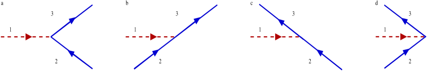
Figure 8: The scattering diagrams for an incoming scalar particle. Particles and momenta run from the left to the right.

Let us now, for comparison, consider the collision term one would usually expect for a scalar particle. In figure 8 we show all tree level processes for an incoming scalar particle given by the interaction Lagrangean

$${\cal L}_{\rm int}=-\bar{\psi}\left(P_{R}y\phi+P_{L}y^{*}\phi^{*}\right)\psi\,.$$ (97)

The matrix element for the first process, the transition of the scalar particle into a fermion-antifermion pair, is

$${\cal M}^{(a)}=-iy\bar{u}_{s^{\prime\prime}}(k^{\prime\prime})P_{R}v_{s^{\prime}}(k^{\prime})\,,$$ (98)

with the notations and conventions for the spinors as used in Ref. ItzyksonZuber:1980 . Calculating the absolute square of the matrix element is done as usual, but with the complication that we do not sum over spins. We find

$$|{\cal M}^{(a)}_{s^{\prime},s^{\prime\prime}}(k^{\prime},k^{\prime\prime})|^{2}=|y|^{2}\,\text{Tr}\left[P_{R}P_{s^{\prime}}(k^{\prime})\mathbin{k\mkern-9.8mu\big{/}}^{\prime}P_{s^{\prime\prime}}(k^{\prime\prime})\mathbin{k\mkern-9.8mu\big{/}}^{\prime\prime}\right]=|y|^{2}F_{s^{\prime}s^{\prime\prime}}(k^{\prime},k^{\prime\prime})\,.$$ (99)

This does not look immediately like an absolute square, since by sending $k^{\prime}$ to $-k^{\prime}$ the sign of the trace changes, but we have to keep in mind that the particles have to be on-shell and the above expression has to be multiplied by the energy-momentum conserving $\delta$-function, $\delta^{4}(k-k^{\prime}-k^{\prime\prime})$, so that eventually (99) is positive definite (one can also check this by actually performing the trace). In a Boltzmann collision term this matrix element appears with a minus sign and is multiplied by the distribution functions $(1-f_{+})(1-f_{-})$ for the outgoing fermion and antifermion, respectively, and $f^{\phi}$ for the incoming scalar particle. We can identify exactly this contribution in the second line within the curly brackets in Eq. (96). Subtracted from it is the inverted process where a fermion and an antifermion annihilate to form a scalar (cf. Ref. Weldon:1983 for similar analyses). In the same way we can find the contribution for the process shown in 8(b), absorption of a scalar by a fermion, and 8(c), absorption by an antifermion, in the first and third line of (96), respectively. Subtracted are the inverted processes, where the scalar comes out. The process shown in 8(d) is kinematically forbidden and therefore does not appear in (96). So the relaxation part of the scalar collision term is exactly what one would expect to find on the right hand side of a classical Boltzmann equation for a scalar particle. It can be shown that the same is true for the fermionic collision term and the Boltzmann equation for a particle with definite spin.

3.2 Relaxation rates

In section LABEL:Boltzmann_transport_equation_for_CP-violating_scalar_densities we derived the kinetic equation (9) for the scalar CP-violating particle density $\delta f_{\phi}$. Obviously, expression (93) for the relaxation term is real, so that the right hand side of the kinetic equation becomes

$$\int_{0}^{\infty}\frac{dk_{0}}{2\pi}2\Big{[}{\cal C}_{\phi}(k)+{\cal C}_{\phi}(-k)\Big{]}\,.$$ (100)

We insert (93) and send $k^{\prime}\rightarrow-k^{\prime}$ and $k^{\prime\prime}\rightarrow-k^{\prime\prime}$ in the second term. The trace stays invariant under this change, so that we find

$$\int_{0}^{\infty}\frac{dk_{0}}{2\pi}2\Big{[}{\cal C}_{\phi}(k)+{\cal C}_{\phi}(-k)\Big{]}$$ (101)

$$= -\frac{|y|^{2}}{2}\,\int\frac{d^{4}k^{\prime}d^{4}k^{\prime\prime}}{(2\pi)^{6}}(2\pi)^{4}\delta^{4}(k+k^{\prime}-k^{\prime\prime})\sum_{s^{\prime}s^{\prime\prime}}F_{s^{\prime}s^{\prime\prime}}(k^{\prime},k^{\prime\prime})2\int_{0}^{\infty}dk_{0}\,$$

$$\delta({k^{\prime}}^{2}-|m|^{2}){\rm sign}(k^{\prime}_{0})\,\,\delta({k^{\prime\prime}}^{2}-|m|^{2}){\rm sign}(k^{\prime\prime}_{0})\,\,\delta(k^{2}-M^{2}){\rm sign}(k_{0})$$

$$\Big{\{}n_{s^{\prime}}(k^{\prime})\left(1-n_{s^{\prime\prime}}(k^{\prime\prime})\right)n^{\phi}(k)-\left(1-n_{s^{\prime}}(k^{\prime})\right)n_{s^{\prime\prime}}(k^{\prime\prime})\left(1+n^{\phi}(k)\right)$$

$$-n_{s^{\prime}}(-k^{\prime})\left(1-n_{s^{\prime\prime}}(-k^{\prime\prime})\right)n^{\phi}(-k)+\left(1-n_{s^{\prime}}(-k^{\prime})\right)n_{s^{\prime\prime}}(-k^{\prime\prime})\left(1+n^{\phi}(-k)\right)\Big{\}}\,.$$

The terms in the last line can be rewritten as antiparticle densities based on the relations (8) and (15). Then we split up the distribution functions into a thermal distribution plus a first order correction term,

$$n^{\phi}(k)=n^{\phi}_{\rm eq}(\hat{k}_{0})+\delta n^{\phi}(k)\,,\quad \quad n^{\phi cp}(k)=n^{\phi}_{\rm eq}(\hat{k}_{0})+\delta n^{\phi cp}(k)$$ (102)

$$n_{s}(k)=n_{\rm eq}(\hat{k}_{0})+\delta n_{s}(k)\,,\quad \quad n_{s}^{cp}(k)=n_{\rm eq}(\hat{k}_{0})+\delta n_{s}^{cp}(k)\,,$$ (103)

and linearize with respect to the correction terms. This constitutes a rather standard linear response approach to equilibration, which is believed to lead to quantitatively correct results for systems close to thermal equilibrium, provided they are not prone to (hydrodynamic turbulent) instabilities HuetKajantieLeighLiuMcLerran:1992 .

Note that the Bose-Einstein and Fermi-Dirac distributions in (102–103) are evaluated at $\hat{k}_{0}=\gamma_{w}(k_{0}+v_{w}k_{z})$, since the wall frame moves with respect to the plasma. Under extensive use of the explicit form of the equilibrium distributions (34), (38) and energy-momentum conservation we can rewrite the first term in curly brackets as

$$\left(1-n_{\rm eq}(\hat{k}_{0}^{\prime\prime})\right)\,n^{\phi}_{\rm eq}(\hat{k}_{0})\,\left(1-n_{\rm eq}(\hat{k}_{0}^{\prime})\right)^{-1}\,\delta n_{s^{\prime}}(k^{\prime})$$

$$\hphantom{XXXXXX}-\;n_{\rm eq}(\hat{k}_{0}^{\prime})\,n^{\phi}_{\rm eq}(\hat{k}_{0})\,{n_{\rm eq}(\hat{k}_{0}^{\prime\prime})}^{-1}\,\delta n_{s^{\prime\prime}}(k^{\prime\prime})$$

$$\hphantom{XXXXXX}+\;n_{\rm eq}(\hat{k}_{0}^{\prime})\,\left(1-n_{\rm eq}(\hat{k}_{0}^{\prime\prime})\right)\,\left(1+n^{\phi}_{\rm eq}(\hat{k}_{0})\right)^{-1}\,\delta n_{\phi}(k)\,.$$ (104)

Exactly the same manipulations are then applied to the $CP$-conjugate densities, and since the equilibrium distributions are spin independent, we can combine the two expressions to

$$\!\!\!\!\!\!\!\int_{0}^{\infty}\frac{dk_{0}}{2\pi}2\Big{[}{\cal C}_{\phi}(k)+{\cal C}_{\phi}(-k)\Big{]}$$ (105)

$$\hphantom{\,}=-|y|^{2}\,\int_{0}^{\infty}dk_{0}\,\int\frac{d^{4}k^{\prime}d^{4}k^{\prime\prime}}{(2\pi)^{6}}(2\pi)^{4}\delta^{4}(k+k^{\prime}-k^{\prime\prime})\sum_{s^{\prime}s^{\prime\prime}}F_{s^{\prime}s^{\prime\prime}}(k^{\prime},k^{\prime\prime})$$

$$\hphantom{\,}\times\;\delta({k^{\prime}}^{2}-|m|^{2})\,{\rm sign}(k^{\prime}_{0})\,\,\delta({k^{\prime\prime}}^{2}-|m|^{2})\,{\rm sign}(k^{\prime\prime}_{0})\,\,\delta(k^{2}-M^{2})\,{\rm sign}(k_{0})n_{\rm eq}(\hat{k}_{0}^{\prime})\big{(}1-n_{\rm eq}(\hat{k}_{0}^{\prime\prime})\big{)}n^{\phi}_{\rm eq}(\hat{k}_{0})$$

$$\hphantom{XX}\times\;\Bigg{\{}\frac{\delta n^{s^{\prime}}(k^{\prime})-\delta n^{-s^{\prime}}_{cp}(k^{\prime})}{n_{\rm eq}(\hat{k}_{0}^{\prime})\big{(}1-n_{\rm eq}(\hat{k}_{0}^{\prime})\big{)}}-\frac{\delta n^{s^{\prime\prime}}(k^{\prime\prime})-\delta n^{-s^{\prime\prime}}_{cp}(k^{\prime\prime})}{n_{\rm eq}(\hat{k}_{0}^{\prime\prime})\big{(}1-n_{\rm eq}(\hat{k}_{0}^{\prime\prime})\big{)}}+\frac{\delta n^{\phi}(k)-\delta n^{\phi}_{cp}(k)}{n^{\phi}_{\rm eq}(\hat{k}_{0})\big{(}1+n^{\phi}_{\rm eq}(\hat{k}_{0})\big{)}}\Bigg{\}}\,.$$

For the fermionic collision term the same procedure can be applied. For the combination of collision terms we eventually need in the kinetic equation (19) for the CP-violating distribution function $\delta f^{a}_{s}$, we find

$$\int_{0}^{\infty}\frac{dk_{0}}{\pi}\Big{[}{\cal K}^{s}_{0}(k)+{\cal K}^{s}_{0}(-k)\Big{]} = -|y|^{2}\,\int\frac{d^{4}k^{\prime}d^{4}k^{\prime\prime}}{(2\pi)^{6}}\sum_{s^{\prime}}\int_{0}^{\infty}dk_{0}\,$$

$$\hskip-57.81621pt\times\;\delta({k^{\prime}}^{2}-|m|^{2})\,{\rm sign}(k^{\prime}_{0})\,\,\delta({k^{\prime\prime}}^{2}-|m|^{2})\,{\rm sign}(k^{\prime\prime}_{0})\,\,\delta(k^{2}-M^{2})\,{\rm sign}(k_{0})$$

$$\hskip-57.81621pt\times\;\bigg{\{}(2\pi)^{4}\delta^{4}(k-k^{\prime}+k^{\prime\prime})F_{ss^{\prime}}(k^{\prime},k^{\prime\prime})n_{\rm eq}(\hat{k}_{0})\left(1-n_{\rm eq}(\hat{k}_{0}^{\prime})\right)n^{\phi}_{\rm eq}(\hat{k}_{0}^{\prime\prime})$$

$$\hskip-43.36243pt+\;(2\pi)^{4}\delta^{4}(k-k^{\prime}-k^{\prime\prime})F_{-s-s^{\prime}}(k^{\prime},k^{\prime\prime})n_{\rm eq}(\hat{k}_{0})\left(1-n_{\rm eq}(\hat{k}_{0}^{\prime})\right)\left(1+n^{\phi}_{\rm eq}(\hat{k}_{0}^{\prime\prime})\right)\bigg{\}}$$

$$\hskip-57.81621pt\times\;\Bigg{\{}\frac{\delta n^{s}(k)-\delta n^{-s}_{cp}(k)}{n_{\rm eq}(\hat{k}_{0})\big{(}1-n_{\rm eq}(\hat{k}_{0})\big{)}}-\frac{\delta n^{s^{\prime}}(k^{\prime})-\delta n^{-s^{\prime}}_{cp}(k^{\prime})}{n_{\rm eq}(\hat{k}_{0}^{\prime})\big{(}1-n_{\rm eq}(\hat{k}_{0}^{\prime})\big{)}}+\frac{\delta n^{\phi}(k^{\prime\prime})-\delta n^{\phi}_{cp}(k^{\prime\prime})}{n^{\phi}_{\rm eq}(\hat{k}_{0}^{\prime\prime})\big{(}1+n^{\phi}_{\rm eq}(\hat{k}_{0}^{\prime\prime})\big{)}}\Bigg{\}}\,.$$

The on-shell $\delta$-functions in these two equations finally project the differences of the deviation functions $\delta n-\delta n_{cp}$ onto the CP-violating distributions $\delta f^{\phi}$ and $\delta f^{a}_{s}$. Of course, the relaxation term of the kinetic equation for $\delta f^{v}_{s}$ is

$$\int_{0}^{\infty}\frac{dk_{0}}{\pi}\Big{[}{\cal K}^{s}_{0}(k)+{\cal K}^{-s}_{0}(-k)\Big{]}\,,$$ (107)

so that here we find $\delta f^{v}_{s}$ as well as on the right hand side. This shows that our kinetic equations (9), (18) and (19) indeed form a closed set of equations, or in other words, that in the relaxation terms of the kinetic equations for the functions $\delta f^{\phi}$, $\delta f^{v}_{s}$ and $\delta f^{a}_{s}$ only these functions themselves do appear. It might be surprising that the relaxation term for the scalar equation contains the fermionic $\delta f^{a}_{s}$, but not $\delta f^{v}_{s}$. The reason for this is the occurrence of the chiral projectors in the interaction Lagrangean.

The relaxation terms that we have discussed so far can be slightly simplified further by performing the sums over those spins that do not appear in the deviation functions. But essentially the form for the rates (105) and (3.2) is as simple as it gets, since we have to integrate over the unknown functions $\delta f$. In the next section we make a fluid Ansatz for the CP-violating distribution functions in order to facilitate numerical solutions of the kinetic equations. The fluid Ansatz expresses the distribution functions in terms of two unknown functions, the chemical potential and the plasma velocity, which, in the stationary limit and in the wall frame, depend only on the spatial $z$-coordinate. The momentum dependence is completely specified by the fluid Ansatz, so that the integrals can be performed and result in interaction rates, which multiply the chemical potentials and plasma velocities of the respective particles in the relaxation term. In appendix D we show the results for the rates for the fermionic quantities in the equation for $\delta f^{a}_{s}$.

The rates we obtain from the one-loop self-energies do not always capture the physically dominant processes responsible for thermalization, however. This is so because we calculate them by forcing the outgoing particles on-shell, which, as a consequence of the energy-momentum conservation, results in a kinematic suppression. Because of this suppression, the rates vanish as any of the (tree level) masses approaches zero and, in general, they are suppressed when the masses are small, that is when $|m|,M\ll T$. The processes described by the one loop approximation in figure 8 constitute absorption and emission processes only. The one-loop approximation completely misses 2-to-2 particle elastic scatterings, which are essential for particle transport.

When the self-energies are approximated at two-loop level, apart from radiative vertex corrections to the one-loop rates, one also captures (tree level) 2-to-2 scatterings rates, which involve off-shell (boson or fermion) exchange. These rates, even though suppressed by two more powers of the coupling constant, do not in general vanish when (any of the) masses approach zero, and hence often dominate thermalization rates in a linear response approximation. For details of thermalization rate calculations starting with an (on-shell) Boltzmann collision term, we refer to Refs. JoyceProkopecTurok:1996 ; JoyceProkopecTurok:1996b ; MooreProkopec:1995 ; ClineJoyceKainulainen:2000+2001 ; ArnoldMooreYaffe:2000+2003 . A complete two-loop treatment of the collision term in the Schwinger-Keldysh formalism is a much more complex task. Nevertheless, we can say something constructive on results of such an undertaking. Indeed, our findings in the first part of this section indicate that the relaxation rates calculated from two-loop self-energies (with distribution functions projected on-shell) can as well be obtained by writing down the naive Boltzmann collision term. Then the scattering amplitude in the collision term is calculated from the 2-to-2 scattering processes, with the important caveat that one must not average over spins (or helicities), as it is usually done in literature, but needs the expressions for the eigenstates of the spin operator (LABEL:Sz,10). (For an example of a helicity-flip rate calculation, which does not involve averaging over helicities, we refer to Appendix B of Ref. JoyceProkopecTurok:1996 .) Recall however that in the super-relativistic limit the spin operator $S_{z}$ approaches the helicity operator (LABEL:helicity-operator) (multiplied by $\hat{\vec{k}}\equiv\vec{k}/|\vec{k}|$). The rates involving particles with a definite spin are therefore in this limit identical to the rates for particles with definite helicities, defined as the projection of spin onto the direction of particle motion.

4 Fluid equations

In Paper I and in the previous sections we have shown that in the semiclassical limit the equations of motion for the scalar and fermionic Wigner functions can be reduced to on-shell conditions and Boltzmann equations. In the first part of this section we closely examine the physical interpretation of the quantities we have been dealing with. Then we examine the highly relativistic limit of our Boltzmann equations for the fermionic particles and compare with the corresponding equations for particles with definite helicity. In the third part we make a fluid Ansatz for the CP-violating distribution functions. The resulting fluid equations are numerically tractable, and we solve them in a very simple model. Finally we reduce the fluid equations to diffusion equations in order to make an estimate of the importance of collisional sources in comparison to the flow term sources.

4.1 Currents

We begin this section by establishing some links between the quantities we dealt with in the previous sections and physical, measurable quantities. The best way to do this is to study various currents. The expectation value of the scalar current operator

$$j_{\phi}(x)=\left<i\phi^{\dagger}(x)\stackrel{{\scriptstyle\leftrightarrow}}{{\!\partial}}\phi(x)\right>$$ (108)

can be written in terms of the Wigner function:

$$j_{\phi}(x)=-(\partial_{u}-\partial_{v})\Delta^{<}(u,v)\Big{|}_{u=v=x}=2\int\frac{d^{4}k}{(2\pi)^{4}}ki\Delta^{<}(k,x)\,.$$ (109)

This current contains information about the density of scalar particles (minus antiparticles) at some space-time point $x$. With the on-shell Ansatz (6) for the scalar Wigner function, the components of the current can be written as

$$j^{0}_{\phi}(x) = \int\frac{d^{3}k}{(2\pi)^{3}}\left[f^{\phi}_{+}(\vec{k},x)-f^{\phi}_{-}(\vec{k},x)-1\right]=\int\frac{d^{3}k}{(2\pi)^{3}}\left[\delta f^{\phi}(\vec{k},x)-1\right]$$ (110)

$$\vec{j}_{\phi}(x) = \int\frac{d^{3}k}{(2\pi)^{3}}\frac{\vec{k}}{\omega_{\phi}}\left[f^{\phi}_{+}(\vec{k},x)-f^{\phi}_{-}(\vec{k},x)\right]\,.$$ (111)

This confirms that $f^{\phi}_{\pm}(\vec{k},x)$ indeed measures the density of scalar particles and antiparticles with momentum $\vec{k}$. The one in the first equation is the vacuum contribution and is therefore ignored.

Similarly, the expectation value of the fermionic current operator

$$j^{\mu}_{\psi}(x)=\left<\bar{\psi}(x)\gamma^{\mu}\psi(x)\right>\,,$$ (112)

which can be rewritten as

$$j^{\mu}_{\psi}(x)=-\text{Tr}[\gamma^{\mu}iS^{<}(x,x)]=-\int\frac{d^{4}k}{(2\pi)^{4}}\text{Tr}\gamma^{\mu}iS^{<}(k,x)\,,$$ (113)

contains information about the density of fermions. A careful consideration of the zero-component and the vector part of this current, and the three-component of the spin-density

$${\cal S}_{z}(x)=\frac{\hbar}{2}\left<\bar{\psi}(x)\gamma^{3}\gamma^{5}\psi(x)\right>$$ (114)

expressed in terms of the on-shell distribution functions (14) and (15) tells that $f_{s\pm}(\vec{k},x)$ measures the density of particles and antiparticles with momentum $\vec{k}$ and spin $s$ (in the direction specified by (LABEL:spin-direction)).

When considering electroweak baryogenesis, the final step in the mechanism that produces the baryon asymmetry is the sphaleron process: it turns the CP-violating flows, whose kinetics we study in this paper, into a net baryon density. To be more precise, the sphaleron acts only on the left handed SU(2) doublets, which are eigenstates of the chirality projector $P_{L}$, but leaves right handed particles unaffected. The densities of left- and right-handed particles

$$j^{0}_{L/R}(x)=\left<\bar{\psi}_{L/R}\gamma^{0}\psi_{L/R}\right>$$ (115)

are linear combinations of the vector density and the axial density $j^{5}=\left<\bar{\psi}\gamma^{0}\gamma^{5}\psi\right>$:

$$j^{0}_{L/R}=\frac{1}{2}\Big{(}j^{0}\mp j^{5}\Big{)}\,.$$ (116)

Finally, the vector density and the axial density are related to the fermionic CP-violating densities (16) and (17) we defined earlier,

$$j^{0}(x) = \sum_{s}\int\frac{d^{3}k}{(2\pi)^{3}}\,\delta f^{v}_{s}(\vec{k},x)$$ (117)

$$j^{5}(x) = \sum_{s}\int\frac{d^{3}k}{(2\pi)^{3}}\,\Big{[}s\frac{k_{z}}{\tilde{\omega}_{0}}\delta f^{a}_{s}(\vec{k},x)+s\frac{k_{z}}{\tilde{\omega}_{s}Z_{s}}f^{\rm eq}_{s}(\vec{k},x)\Big{]}\,,$$ (118)

which explains the terminology. We omitted the vacuum contribution to the vector density. It might seem strange that the equilibrium distribution contributes to the axial density, but this is just a consequence of defining $f^{\rm eq}$ as the projection of $n_{\rm eq}$ to the mass shell $\omega_{s}$. Had we defined $f^{\rm eq}=n_{\rm eq}(\omega_{0})$, then the axial density would be expressed by $\delta f^{a}_{s}$ alone, but in turn there would be additional source terms in the Boltzmann equation for this function.

Both CP-violating densities contribute to the left-handed density, so both could lead to baryon production. Recall however that in the equation (18) for $\delta f^{v}_{s}$ there is no source, neither from the flow term nor from the collision term. We therefore assume that this density, and consequently the vector density, vanishes and then we have $j^{0}_{L}=-j^{0}_{R}=-j^{5}/2$. The source in the equation for $\delta f^{a}_{s}$ is proportional to spin, so that any contribution in $\delta f^{a}_{s}$ caused by this source is also proportional to spin. Therefore the spin summation in the expression for $j^{5}$ does not cancel the contributions against each other, but adds them up, wherefore the source in the equation for $\delta f^{a}_{s}$ eventually is an effective source for electroweak baryogenesis. The source in the scalar equation can contribute to baryogenesis only indirectly. It first creates a CP-violating scalar density, which then may be transferred into the fermionic CP-violating distribution function via the collision term of the scalar kinetic equation.

Finally, a word on mixing particles. The sphaleron acts on the particles in the electroweak interaction basis, while the densities we are dealing with are those of particles in the mass basis. So in principle we would have to rotate these densities into the interaction basis. This is not necessary, however: the sphaleron is effective only in the symmetric phase, where the Higgs vacuum expectation value vanishes, and in those regions of the bubble wall where the expectation value is small. But for a vanishing Higgs expectation value the mass basis and the interaction basis coincide. So we can compute the contribution to the axial density for each particle, using the densities in the mass eigenbasis, and sum them up.

In the following we will not consider the equilibrium contribution to the axial density any further, another consequence of the sphaleron’s refusal to work anywhere else than in the symmetric phase. Electroweak baryogenesis is most effective when there are CP-violating flows that are efficiently transported away from the wall into the symmetric phase, where they are converted into a baryon asymmetry. The equilibrium contribution to the axial density, however, sits right on top of the wall and does not participate in diffusion.

4.2 Spin or helicity?

In the highly relativistic limit we can approximate $\tilde{\omega}_{0}$ by $|k_{z}|$. In this case the density of left-handed particles can be written as

$$j^{0}_{L}=\frac{1}{2}\sum_{s}\int\frac{d^{3}k}{(2\pi)^{3}}\left(1-\frac{sk_{z}}{|k_{z}|}\right)\left(\delta f_{s+}(\vec{k})-\delta f_{-s-}(\vec{k})\right)\,,$$ (119)

where we allowed for a possible contribution from the vector density. But this is of course precisely the density of particles with negative helicity minus the density of antiparticles with positive helicity (for massless antiparticles chirality is opposite to helicity):

$$j^{0}_{L}\propto\int_{0}^{\infty}dk_{z}\left(\delta f_{-+}-\delta f_{+-}\right)+\int_{-\infty}^{0}dk_{z}\left(\delta f_{++}-\delta f_{--}\right)\,.$$ (120)

In fact, in every earlier work on EWB that used the WKB method, the Boltzmann equations were written directly for the densities of particles with a definite helicity (or chirality). The equation we derived for spin states is

$$\big{(}\partial_{t}+\vec{v}_{0i}\cdot\nabla_{\vec{x}}+F_{0i}\partial_{k_{z}}\big{)}\delta f^{a}_{si}+s{\cal S}_{i}=\int_{0}^{\infty}\frac{dk_{0}}{\pi}\Big{[}{\cal K}^{s}_{0i}(k)-{\cal K}^{cp-s}_{0i}(k)\Big{]}_{relax}\,,$$ (121)

where ${\cal S}_{i}$ denotes all sources, both those from the flow term (LABEL:boltzmann:deltaf-a_source–LABEL:boltzmann:deltaf-a_even) and from the collision term (77–78), while on the right hand side only the relaxation part of the collision term is left. It is now not difficult to break this equation up into four equations with $s=\pm 1$ and $k_{z}>0$ and $k_{z}<0$, respectively, and then combine those pieces with opposite $s$ and $k_{z}$ to the equation

$$\big{(}\partial_{t}+\vec{v}_{0i}\cdot\nabla_{\vec{x}}+F_{0i}\partial_{k_{z}}\big{)}\delta f_{hi}+h\,\text{sign}[k_{z}]\,{\cal S}_{i}=\int_{0}^{\infty}\frac{dk_{0}}{\pi}\Big{[}{\cal K}^{h}_{0i}(k)-{\cal K}^{cp-h}_{0i}(k)\Big{]}_{relax}\,,$$ (122)

where $\delta f_{hi}$ is the density of particles with helicity $h$ minus the density of antiparticles with opposite helicity, precisely the quantity needed for the left-handed density (120). Formally, this equation for helicity states has almost identical appearance as the one used in the heuristic WKB approach to baryogenesis (the classical force in the flow of the CP-violating density is usually omitted in these works), where the CP-violating source ${\cal S}_{i}$ is approximated by the semiclassical force. What this analysis really shows is that the WKB approach, combined with a good guess work, which involves a correct calculation of the dispersion relation (obtained by transforming from canonical to kinetic momentum), and the right modus of insertion of the dispersion relation into the kinetic equation, can lead to the correct CP-violating force. However, we emphasize that no work using the WKB approach has so far gotten the full source completely right. Another point is that the interpretation of $h$ as helicity really makes sense only in the highly relativistic limit, or equivalently, in the symmetric phase, in which the tree level masses vanish.

Furthermore, it is important to note that the explicit form of the source found in those works differs from our result: first, the contribution from the flow term to the source there contains only the semiclassical force $\delta F_{i}$ from (LABEL:boltzmann:definitions), but misses the other contributions we found. In section 4.4 we make a numerical estimate of the importance of these terms. Second, the semiclassical WKB method is not in principle suitable to calculate the source that originates from the collision term.

4.3 Fluid equations

We now have the Boltzmann equations for the CP-violating distribution functions, and we know how to interpret them in terms of densities and currents and what is their role in the creation of a baryon asymmetry. A direct numerical solution of the Boltzmann equations (9) fails due to their complexity, however, at least at present. So we have to rely on approximations to the full Boltzmann equations. A very convenient and with respect to the application to EWB quite popular approximation is a fluid Ansatz for the distribution functions JoyceProkopecTurok:1996 :

$$f_{si\pm}=\frac{1}{{\rm e}^{\beta(\omega_{si}+v_{w}k_{z}-\mu^{s}_{i\pm}+u^{s}_{i\pm}k_{z})}+1}$$ (123)

for the fermions, and an analogous expression without spin indices for the scalar distributions. This form mimics the equilibrium distribution, but the chemical potential $\mu$ and the plasma velocity $u$, which are only functions of the spatial coordinates, allow for local fluctuations in the density and velocity of the plasma. In the given form the velocity perturbation accounts only for a net motion of particles in $z$-direction. Because of the planar symmetry of the wall, this should be sufficient. The term including the wall velocity is due to the movement of the wall frame in the plasma rest frame. With the Ansatz (123) the momentum dependence is explicit, such that, upon integrating the Boltzmann equations over momentum, only spatial dependencies remain.

The CP-violating chemical potential and the velocity perturbation are caused by the interaction with the wall and hence are implicitly of first order in gradients. When we expand the fluid Ansatz (123), keeping only terms linear in $\mu$, $u$ and $v_{w}$, and compare it with our decomposition (LABEL:distribution-fn_fsi_decompose) of the fermionic distribution function, leaving aside the CP-even correction, we can identify

$$\delta f_{si\pm}=-\beta f_{0i}(1-f_{0i})\left[1-\beta v_{w}k_{z}(1-2f_{0i})\right]\left(-\mu_{si\pm}+k_{z}u_{si\pm}\right)\,,$$ (124)

where $f_{0i}=1/({\rm e}^{\beta\omega_{0i}}+1)$, $\omega_{0i}=(\vec{k}^{2}+|m_{d}|_{i}^{2})^{1/2}$. The form (17) of the CP-violating distribution $\delta f^{a}_{s}$ then suggests to define

$$\mu_{si} \equiv \mu_{si+}-\mu_{-si-}$$ (125)

$$u_{si} \equiv u_{si+}-u_{-si-}\,.$$ (126)

We insert the fluid Ansatz into the Boltzmann equation for the fermionic CP-violating density $\delta f^{a}_{s}$ and keep all terms up to second order in gradients and up to first order in $v_{w}$. Then we take the zeroth and first moment with respect to $k_{z}$, that is we multiply by $1$ and $k_{z}/\omega_{0}$, respectively, and integrate over the momenta. Since the flow term source is even in $k_{z}$, it contributes to the zeroth moment equation:

$$I_{00,i}\beta\dot{\mu}_{si}+v_{w}J_{20,i}\dot{u}_{si}-v_{w}J_{21,i}\beta\mu_{si}^{\prime}-I_{21,i}u_{si}^{\prime}$$ (127)

$$+v_{w}J_{01,i}\beta^{3}\frac{{|m_{d}|_{i}^{2}}^{\prime}}{2}\mu_{si}+I_{01,i}\beta^{2}\frac{{|m_{d}|_{i}^{2}}^{\prime}}{2}u_{si}+\beta^{3}\int\frac{d^{3}k}{(2\pi)^{3}}s{\cal S}_{i}^{\rm flow}(\vec{k})$$

$$= -\sum_{s^{\prime}i^{\prime}}\Big{(}\beta\Gamma^{0\mu}_{si,s^{\prime}i^{\prime}}\mu_{s^{\prime}i^{\prime}}+v_{w}\Gamma^{0u}_{si,s^{\prime}i^{\prime}}u_{s^{\prime}i^{\prime}}\Big{)}-\sum_{i^{\prime}}\Big{(}\beta\Gamma^{0\mu}_{i,i^{\prime}}\mu_{i^{\prime}}+v_{w}\Gamma^{0u}_{i,i^{\prime}}u_{i^{\prime}}\Big{)}\,.$$

In the following we do not consider the contribution (LABEL:boltzmann:deltaf-a_even) from the CP-even distribution function $\delta f_{i}^{\rm even}$ to ${\cal S}_{i}^{\rm flow}$, which in principle can be of the same order as (LABEL:boltzmann:deltaf-a_source). The source from the collision term is odd in $k_{z}$ and therefore appears in the first moment equation:

$$v_{w}J_{21,i}\beta\dot{\mu}_{si}+I_{21,i}\dot{u}_{si}-I_{22,i}\beta\mu_{si}^{\prime}-v_{w}J_{42,i}u_{si}^{\prime}$$ (128)

$$+v_{w}J_{22,i}\beta^{2}{|m_{d}|_{i}^{2}}^{\prime}u_{si}+\beta^{3}\int\frac{d^{3}k}{(2\pi)^{3}}\frac{k_{z}}{\omega_{0}}s{\cal S}_{i}^{\rm coll}(\vec{k})$$

$$= -\sum_{s^{\prime}i^{\prime}}\Big{(}v_{w}\beta\Gamma^{1\mu}_{si,s^{\prime}i^{\prime}}\mu_{s^{\prime}i^{\prime}}+\Gamma^{1u}_{si,s^{\prime}i^{\prime}}u_{s^{\prime}i^{\prime}}\Big{)}-\sum_{i^{\prime}}\Big{(}v_{w}\beta\Gamma^{1\mu}_{i,i^{\prime}}\mu_{i^{\prime}}+\Gamma^{1u}_{i,i^{\prime}}u_{i^{\prime}}\Big{)}\,.$$

Here dots denote the derivative with respect to time, primes are $z$-derivatives, and we introduced the dimensionless integrals

$$I_{ab,i} = \beta^{3+a-b}\int\frac{d^{3}k}{(2\pi)^{3}}f_{0i}(1-f_{0i})\frac{k^{a}_{z}}{\omega^{b}_{0i}}$$ (129)

$$J_{ab,i} = \beta^{3+a-b}\int\frac{d^{3}k}{(2\pi)^{3}}f_{0i}(1-f_{0i})(1-2f_{0i})\frac{k^{a}_{z}}{\omega^{b}_{0i}}\,.$$ (130)

With the fluid Ansatz the momentum dependence of the $\delta f^{a}_{s}$ and $\delta f^{\phi}$ is specified, so that the integrals in the relaxation term (3.2) can be performed, leading to the relaxation rates $\Gamma_{si,s^{\prime}i^{\prime}}$ and $\Gamma_{i,j}$, which connect different fermionic species with each other and fermionic particles with scalar particles, respectively. Some explicit expressions for the rates calculated in our one-loop approximation can be found in appendix D. Note however that with our conventions the above fluid equations imply that the actual rates, by which the chemical potential and the fluid velocity perturbations are attenuated, are given by $\Gamma^{0\mu}_{si,s^{\prime}i^{\prime}}/I_{00,i}$ and $\Gamma^{1u}_{si,s^{\prime}i^{\prime}}/I_{21,i}$, respectively, which are about one order of magnitude larger than $\Gamma^{0\mu}_{si,s^{\prime}i^{\prime}}$ and $\Gamma^{1u}_{si,s^{\prime}i^{\prime}}$.

The equations for the scalar particles can be obtained from the ones for fermions in a simple way: one has to replace $|m|^{2}$ by $M^{2}$, remove the source from the flow term, replace the collisional source by the scalar one, use the appropriate relaxation rates for scalars, and replace the coefficients $I$ and $J$ by their scalar counterparts, whereby the Bose-Einstein distribution replaces the Fermi-Dirac function.

The fluid equations (127–128) are well suited for a numerical treatment. They consist of a system of first order differential equations, which is a comparatively simple problem. Note that only the time- and the $z$-derivative have survived. This is a consequence of the fluid Ansatz, which in the above form effectively allows for spatial variations only in the $z$-direction. Since in the wall frame the mass depends only on the $z$-coordinate, the problem is stationary in essence and we could drop the time derivative. We argued in the beginning of section LABEL:The_3+1_dimensional_(moving)_frame that keeping the time derivative could allow a treatment of non-equilibrium initial conditions. But in order not to violate the spin, which is conserved by the symmetry of the problem, these initial conditions have to have quite a special form, given by equation (LABEL:S<-tildeS<), so that their physical relevance is at best limited. Keeping the time derivative is however a convenient tool to solve the equations. At a first sight it seems to be simpler to have only ordinary differential equations instead of partial ones. But to solve these ordinary equations is actually quite tricky, since boundary conditions at infinity have to be satisfied: at sufficiently large distances apart from the wall we expect the system to be in chemical equilibrium. Starting with some initial values at one side of the wall usually does not lead to the correct chemical equilibrium on the other side, so that the initial value has to be fine-tuned. A simpler procedure is to keep the time derivative and thus simulate relaxation of the system toward a stationary state, starting from some well-chosen initial functions $\mu_{0}(z)$ and $u_{0}(z)$. Because of the interplay between the dissipative effects in the relaxation term on the one hand and the sources on the other, this procedure leads to stable stationary solutions relatively fast.

Once the solutions of the fluid equations are known, the axial density can be calculated. Inserting (124) into (118) leads to the relation

$$j^{5}=-\sum_{s}s\int\frac{d^{3}k}{(2\pi)^{3}}\beta f_{0}(1-f_{0})\frac{k_{z}^{2}}{\tilde{\omega}_{0}}\Big{(}u_{s}+v_{w}\beta(1-2f_{0})\mu_{s}\Big{)}\,.$$ (131)

It is interesting that the main contribution to the axial density here comes from the plasma velocity, since the chemical potential is suppressed by an extra factor $v_{w}$.

4.4 Solving the fluid equations

We now solve the fluid equations in a toy model consisting of one fermionic particle species. Despite of the marked simplicity of this model, the explicit solution of the equations will be instructive, and in particular will help to answer three questions. First, we would like to know how big is the collisional source (78), when compared to the flow term source (LABEL:boltzmann:deltaf-a_source). Since these sources appear in different equations, a direct comparison is not possible. But we can study the influence of the presence or absence of the collisional source on the axial density. This should allow us to judge if this contribution could be important in an actual calculation of EWB in a realistic model. Second, we found that previous work based on the WKB method missed a part of the flow term source (LABEL:boltzmann:deltaf-a_source). Are the new terms relevant? And finally, we have seen that in the highly relativistic limit on the level of Boltzmann equations the use of spin states or helicity states is equivalent. As soon as an approximation to these equations is made, however, as for example the fluid Ansatz, differences occur. We can solve the fluid equations in both pictures, compute the axial density and compare the results, in order to study by how much the equivalence between spin and helicity states is broken on the level of fluid equations.

Figure 9: The axial density generated by the flow term source, the “old” flow term source, and the collisional source, respectively, for different values of the fermionic mass parameter. The pictures on the left hand side, computed with the rates (133), show no diffusion, while in the pictures on the right, computed with (134), the effects of diffusion can be seen. For this choice of parameters the contribution of the collisional source is negligible. The difference between the results for the two flow term sources is apparent. The bubble wall with width $L_{w}=10/T$ sits at $z=0$, the broken phase is at the left. Note the different scales of the $z$-axes.

The bubble wall can be modeled by a hyperbolic tangent

$$|m|=m_{0}\frac{1}{2}\Big{(}1-\mbox{tanh}\frac{z}{L_{w}}\Big{)}\,,\quad\theta=\theta_{0}\frac{1}{2}\Big{(}1-\mbox{tanh}\frac{z}{L_{w}}\Big{)}$$ (132)

for both the absolute value and the phase of the fermionic mass. Here $L_{w}$ characterizes the wall thickness. In contrast to the fermionic mass parameter $m_{0}$, which influences the form of the source and therefore also the form of the result, $\theta_{0}$ is simply a common prefactor to all source terms and therefore only scales the result of the computation. We choose $\theta_{0}=0.1$. The width of the bubble wall is set to $L_{w}=10/T$, a typical value for the MSSM, and the wall velocity is chosen to be $v_{w}=0.1$. We want to investigate the collisional source for the fermionic equations, so the system must also contain scalar particles. But since we are interested only in the dynamics of the fermionic particles, we assume a thermal distribution for the scalars. Both fermions and scalars get their masses from the interaction with the Higgs field, and therefore the scalar mass is proportional to $|m|$. To keep things simple, we set all relaxation rates in (127) and (128) to zero, except of $\Gamma^{0\mu}_{ss}$ and $\Gamma^{1u}_{ss}$. For these rates we use two different sets of values,

$$\Gamma^{0\mu}_{ss}=T/25\,,\quad\Gamma^{1u}_{ss}=T/20\,,\quad s=\pm 1\,,$$ (133)

which are so big that there will essentially be no diffusion of particles in front of the wall, and

$$\Gamma^{0\mu}_{ss}=T/120\,,\quad\Gamma^{1u}_{ss}=T/100\,,\quad s=\pm 1\,,$$ (134)

which are small enough to have a notable diffusion. Note that both fluid equations contain the time derivative of the chemical potential and of the plasma velocity. We first build linear combinations of these two equations, such that we obtain one equation which contains only the time derivative of $\mu$, and another equation in which only the time derivative of $u$ appears. The temporal evolution of these equations can then be simulated numerically in a straightforward manner, where we choose $\mu$ and $u$ to be identical to zero as initial values. We emphasize again that this evolution is a physical temporal evolution only for the very special initial conditions (LABEL:S<-tildeS<). But in any case it is a convenient way of obtaining the solutions of the ordinary differential equations in $z$, which emerge by setting the time derivatives to zero, without having to worry about boundary conditions.

Figure 10: The effects of diffusion can be nicely seen here, where we plotted the axial density produced by the same source, but with different sets of relaxation rates, (133) and (134). For comparison we also show the flow source. The axial density computed with the larger relaxation rates is not transported into the symmetric phase, but sits right on top of the source, while for the small rates a diffusion tail is clearly visible. For small masses diffusion is more efficient.

To address the first two questions we mentioned above, we solve the fluid equations for three different cases: with the flow term source, with the “old” flow term source, that means using only the first term of (LABEL:boltzmann:deltaf-a_source), as it was done in the WKB calculations, and with the collisional source only. The computation is done for three different values of the fermionic mass parameter $m_{0}$, and for the collisional source we set $M=3.0|m|$ and use $|y|^{2}=0.1$ for the coupling constant. In figure 9 the resulting axial density is shown as a function of the $z$-coordinate. On the left hand side are the results obtained by using the larger relaxation rates (133), while for the pictures on the right hand side the smaller rates (134) have been used. For the parameters chosen, the collisional source has no notable effect. Repeating the calculation with different wall velocities and scalar masses does not increase the collisional contribution significantly. Note that for smaller relaxation rates not only a diffusion tail develops, but the amplitude of the axial density grows, too.

The axial density originating in the “old” flow term source overestimates the one from the true flow term source, with a difference increasing with the mass parameter. While for small mass parameters $m_{0}<T$ both sources give about the same result, the difference becomes significant for larger masses. We conclude that a computation of EWB with the correct flow term source will most probably lead to different results for the baryon density than the WKB calculations.

In order to illustrate the difference between the situations with and without effective diffusion, we show in figure 10 the axial densities calculated with the two sets of rates (133) and (134) in direct comparison.

Figure 11: The axial density computed by solving the fluid equations for spin states and helicity states, respectively. The results are very similar, but for both values of the fermion mass there is a clearly visible difference.

Working with spin states instead of helicity states leads to two important changes on the level of the fluid Ansatz. Because in the Boltzmann equation (122) the source is multiplied by $\mbox{sign}(k_{z})$, the flow term source for helicity states will appear in the first moment equation, and the collisional source will go into the zeroth moment equation, just opposite to the fluid equations for spin states. The other difference concerns the axial density, which in terms of chemical potential and plasma velocity now reads

$$j^{5}=\sum_{h}h\int\frac{d^{3}k}{(2\pi)^{3}}\beta f_{0}(1-f_{0})\Big{(}\mu_{h}+v_{w}\beta(1-2f_{0})u_{h}\Big{)}\,.$$ (135)

Compared to (131) for spin states, the roles of chemical potential and plasma velocity have changed, in a way. The question is now, whether the effects of both of these changes cancel each other. So we solve the fluid equations also for helicity states and show the result for the axial density in figure 11, in direct comparison with the density obtained by working with spin states. One can see that the results differ by about ten percent. For small masses the fluid equations for spin states produce a larger axial density, for high masses the equations for helicity states produce the larger result. Since both cases are an approximation to the full Boltzmann equations, this difference can to some extent also be regarded as an estimate of the error one makes by going from Boltzmann to fluid equations.

4.5 Diffusion equation and sources

Here we make a rough analytic comparison between the flow and collision term sources. In the stationary limit and neglecting the terms of order $v_{w}^{2}\ll 1$ (as usually, in the wall frame), Eqs. (127–128) can be recast as

$$\!\!\!\!\!\!\!\!\!\!\!\!I_{21,i}u_{si}^{\prime}-I_{01,i}\beta^{2}\frac{{|m_{d}|_{i}^{2}}^{\prime}}{2}u_{si}-v_{w}J_{01,i}\beta^{3}\frac{{|m_{d}|_{i}^{2}}^{\prime}}{2}\mu_{si}-\beta^{3}\!\int\frac{d^{3}k}{(2\pi)^{3}}s{\cal S}^{\rm flow}_{i}$$

$$= \!\sum_{s^{\prime}i^{\prime}}\Big{[}\Gamma^{0\mu}_{si,s^{\prime}i^{\prime}}\beta\mu_{s^{\prime}i^{\prime}}-v_{w}\Big{(}\Gamma^{1u}_{si,s^{\prime}i^{\prime}}\!-\!\frac{J_{21,i}}{I_{22,i}}\Gamma^{0u}_{si,s^{\prime}i^{\prime}}\Big{)}u_{s^{\prime}i^{\prime}}\Big{]}+\!\sum_{i^{\prime}}\Big{[}\Gamma^{0\mu}_{i,i^{\prime}}\beta\mu_{i^{\prime}}-v_{w}\Big{(}\Gamma^{1u}_{i,i^{\prime}}\!-\!\frac{J_{21,i}}{I_{22,i}}\Gamma^{0u}_{i,i^{\prime}}\Big{)}u_{i^{\prime}}\Big{]}$$

$$\!\!\!\!\!\!\!\!\!\!\!\!\!\!I_{22,i}\beta\mu_{si}^{\prime}+v_{w}\Big{(}\frac{I_{01,i}J_{42,i}}{2I_{21,i}}\!-\!J_{22,i}\Big{)}\beta^{2}{|m_{d}|_{i}^{2}}^{\prime}u_{si}-\beta^{3}\!\int\frac{d^{3}k}{(2\pi)^{3}}\frac{k_{z}}{\omega_{0i}}s{\cal S}^{\rm coll}_{i}$$

$$= \sum_{s^{\prime}i^{\prime}}\Big{[}v_{w}\Big{(}\Gamma^{1\mu}_{si,s^{\prime}i^{\prime}}\!-\!\frac{J_{42,i}}{I_{21,i}}\Gamma^{0\mu}_{si,s^{\prime}i^{\prime}}\Big{)}\beta\mu_{s^{\prime}i^{\prime}}+\Gamma^{1u}_{si,s^{\prime}i^{\prime}}u_{s^{\prime}i^{\prime}}\Big{]}+\sum_{i^{\prime}}\Big{[}v_{w}\Big{(}\Gamma^{1\mu}_{i,i^{\prime}}\!-\!\frac{J_{42,i}}{I_{21,i}}\Gamma^{0\mu}_{i,i^{\prime}}\Big{)}\beta\mu_{i^{\prime}}+\Gamma^{1u}_{i,i^{\prime}}u_{i^{\prime}}\Big{]}\,,$$

where we kept only those sources which are not suppressed by the wall velocity. (Recall that the sources ${\cal S}^{\rm flow}_{i}$ and ${\cal S}^{\rm coll}_{i}$ are both linear in $v_{w}$.) From Eq. (4.5) we can easily write an expression for the fluid velocity,

$$u_{si}\! = \!\frac{1}{\Gamma^{1u}_{si,si}+v_{w}\Big{(}J_{22,i}\!-\!\frac{I_{01,i}J_{42,i}}{2I_{21,i}}\Big{)}\beta^{2}{|m_{d}|_{i}^{2}}^{\prime}}\Bigg{[}I_{22,i}\beta\mu_{si}^{\prime}-\!\sum_{s^{\prime}i^{\prime}}v_{w}\Big{(}\Gamma^{1\mu}_{si,s^{\prime}i^{\prime}}\!-\!\frac{J_{42,i}}{I_{21,i}}\Gamma^{0\mu}_{si,s^{\prime}i^{\prime}}\Big{)}\beta\mu_{s^{\prime}i^{\prime}}$$ (138)

$$\hskip 144.54pt+v_{w}\frac{J_{42,i}}{I_{21,i}}\beta^{3}\!\int\frac{d^{3}k}{(2\pi)^{3}}s{\cal S}^{\rm flow}_{i}-\beta^{3}\!\int\frac{d^{3}k}{(2\pi)^{3}}\frac{k_{z}}{\omega_{0i}}s{\cal S}^{\rm coll}_{i}$$

$$\hskip 144.54pt-{\sum_{s^{\prime}i^{\prime}}}^{\prime}\Gamma^{1u}_{si,s^{\prime}i^{\prime}}u_{s^{\prime}i^{\prime}}-\sum_{i^{\prime}}\Big{[}v_{w}\Big{(}\Gamma^{1\mu}_{i,i^{\prime}}\!-\!\frac{J_{42,i}}{I_{21,i}}\Gamma^{0\mu}_{i,i^{\prime}}\Big{)}\beta\mu_{i^{\prime}}+\Gamma^{1u}_{i,i^{\prime}}u_{i^{\prime}}\Big{]}\Bigg{]}\,,\qquad$$

and similarly for $\mu_{si}$. Upon inserting Eq. (138) and its derivative into the continuity equation (4.5), we get a rather complicated second order diffusion equation for the chemical potential, from which we list just a few relevant terms,

$$\!\!\!\!\!\!\!\!\!\!D_{si}\mu_{si}^{\prime\prime}-v_{w}D_{si}\sum_{s^{\prime}i^{\prime}}\Big{(}\frac{\Gamma^{1\mu}_{si,s^{\prime}i^{\prime}}}{I_{22,i}}-\frac{J_{42,i}}{I_{22,i}I_{21,i}}\Gamma^{0\mu}_{si,s^{\prime}i^{\prime}}\Big{)}\beta\mu_{si}^{\prime}$$ (139)

$$\!\!\!\!\!\!\!\!\!-\frac{D_{si}}{I_{22,i}}\beta^{2}\int\frac{d^{3}k}{(2\pi)^{3}}\frac{k_{z}}{\omega_{0i}}s{{\cal S}^{\rm coll}_{i}}^{\,\prime}-\frac{I_{01,i}}{I_{00,i}}\beta^{4}\frac{{|m_{d}|^{2}}^{\prime}}{2}\int\frac{d^{3}k}{(2\pi)^{3}}\frac{k_{z}}{\omega_{0i}}s{\cal S}^{\rm coll}_{i}-\frac{1}{I_{00,i}}\beta^{2}\int\frac{d^{3}k}{(2\pi)^{3}}s{\cal S}^{\rm flow}_{i}+..=0\,,\quad$$

where we defined a diffusion coefficient

$$D_{si}\equiv\frac{I_{21,i}I_{22,i}}{I_{00,i}}\frac{1}{\Gamma^{1u}_{si,si}}+O(v_{w})\,.$$ (140)

\psfrag{Lx}[r]{$|m|/T$}\psfrag{Ly}[r][1][-90]{$\Gamma^{1u}_{s,s}/T$}\includegraphics[width=252.94499pt,angle={-90}]{B_pics/gammaU1pp.eps}

Figure 12: The rate $\Gamma^{1u}_{s,s}$ as a function of the fermion mass $|m|$. The scalar mass $M$ is a multiple of $|m|$. At the ratio $M/|m|$ increases, the rate peaks at an asymptotic value $\Gamma^{1u}_{s,s}\rightarrow(0.9-1.0)\times 10^{-3}T$. The spin-flip rate $\Gamma^{1u}_{s,-s}$ is negative and smaller by a factor four, approximately.

We can neglect the contribution of the collisional source term $\propto{|m_{d}|_{i}^{2}}^{\prime}$, unless the diffusion constant is very small and $|m_{d}|_{i}\ll T$. From Eq. (140) it is then clear that as the diffusion parameter $D_{si}$ grows (or equivalently, when $\Gamma^{1u}_{si,si}$ becomes small), the collisional source becomes more and more important. To give a rough quantitative comparison between the sources, we first note that the flow and the collision term sources (LABEL:parametric-flow-source), (85) can be approximated by

$$\beta^{4}\!\int\frac{d^{3}k}{(2\pi)^{3}}{\cal S}_{i}^{\rm flow} \sim 2\times 10^{-6}\frac{m_{0}^{2}}{T^{2}}\Big{(}-{\cal I}_{a}+\frac{m_{0}^{2}}{T^{2}}{\cal I}_{b}\Big{)}$$ (141)

$$\beta^{4}\!\int\frac{d^{3}k}{(2\pi)^{3}}\frac{k_{z}}{\omega_{0i}}{\cal S}_{i}^{\rm coll} \sim 2\times 10^{-7}{\cal I}\,,$$ (142)

where we made use of $\partial_{z}\sim 1/L=T/10$, $\theta\sim\theta_{0}=0.1$, $|m_{d}|_{i}\sim m_{0}$, and $v_{w}=0.1$. Now from figures LABEL:figure:flow-source and 7 we see that ${\cal I}_{a}$ and ${\cal I}_{b}$ peak at about one, and are typically one order of magnitude larger than ${\cal I}$, and we conclude that the flow term source (141) is typically about two orders of magnitude larger than the collision term source (142). When viewed as sources in the diffusion equation (139), we first observe that both sources appear at second order in gradients, and are hence suppressed as $1/L_{w}^{2}$, so changing the wall thickness $L_{w}$ should not affect much the relative strength of the sources. Analogously, the relative strength of the sources is not changed by changing the wall velocity $v_{w}$, Yukawa coupling $|y|$, or CP-violating phase $\theta$. Second, making a comparison of the collisional and flow term sources in Eq. (139) at a maximum $|m_{d}|_{i}\sim T$ leads to the conclusion that the sources are comparable when the diffusion constant becomes $D_{si}\sim 300T^{-1}$, such that $\Gamma^{1u}_{si,si}\sim 0.03D_{si}^{-1}\sim 10^{-4}T$ is the rate below which the collisional source should dominate . A self consistent quantitative comparison of the two sources can be inferred from the above analysis and Figure 12, where we show the rate $\Gamma^{1u}_{si,si}$ as a function of the masses $|m_{d}|_{i}$ and $M_{i}$. In the parameter range where the sources peak, $|m_{d}|_{i}\simeq T$ and $M_{i}\simeq(3-4)T$, the rate $\Gamma^{1u}_{si,si}\simeq(3-5)\times 10^{-4}T$. This then implies that, when compared with the flow term source, in the region of parameter space where both sources peak, the collisional source is a few times smaller. This collisional source suppression can be attributed to a phase space suppression of ${\cal S}_{i}^{\rm coll}$, to which only particles with relatively small momenta contribute, which are not so numerous. We expect that a similar conclusion can be reached when higher order loop processes are considered, both as regards to the collisional source as well as diffusion constant contributions.

5 Conclusion

With the present paper we complete our work on a controlled first principle derivation of transport equations for chiral fermions Yukawa-coupled to complex scalars by a discussion of the collision term, whereby we approximate the self-energies by the one-loop expressions.

We calculate, from first principles, the CP-violating source appearing in the collision term of the fermionic kinetic equation. This represents a first calculation in which both semiclassical and spontaneous sources are obtained within one formalism. We also present a first computation of a CP-violating source from the scalar collision term, which arises from nonlocal fermion loop Wigner functions, and can be traced to the CP-violating split in the dispersion relation for fermions. Next, we derive the fluid equations associated to the Boltzmann equations found in Paper I and solve them (by a novel method) for a simple case, including only fermionic particles, which allows us to make a comparison between different sources. It turns out that the collisional source is subdominant when compared with the semiclassical source coming from the semiclassical force in the flow term of the fermionic kinetic equation, unless the fermions diffuse very efficiently.

We discuss the relation between the helicity and the spin quasiparticle states and show that in a highly relativistic limit the Boltzmann equation for spin quasiparticles reduces to the one for helicity quasiparticles. Fluid equations are, however, not the same. In particular, we show that in the fluid equations for spin quasiparticles the semiclassical force sources the continuity equation, while the collision term sources the Euler equation; exactly the opposite is true for the fluid equations of helicity quasiparticles.

The question of thermalization rates in the collision term of the Kadanoff-Baym equations is also addressed. We calculate the rates with the one-loop self-energies, for which only scalar absorption and emission processes are taken into account. We point out at the shortcomings of these rates: as a consequence of the energy momentum conservation enforced in the on-shell limit, the rates are suppressed for small masses, and vanish in the massless limit. By establishing a relation to more standard rates calculated with helicity states, we outline how one could approximate scattering rate calculations from the Kadanoff-Baym equations with two-loop self-energies, which are needed for the derivation of quantitatively correct fluid equations.

We conclude by making a few comments on further directions of the research presented here and in Paper I. Solving the Kadanoff-Baym equations with the self-energies truncated at two-loop order, needed for modeling baryogenesis at a first order electroweak phase transition, would require a significantly more effort than what was needed in this work, and thus would be justified only when quantitative consistency checks of a particle physics model would be needed. Testing the accuracy of the fluid equations based on the Kadanoff-Baym equations with one-loop self-energies is feasible, and should be performed. Furthermore, it would be of interest to develop a basis independent formalism for mixing fermions valid to order $\hbar$ in a derivative expansion, and in particular to study the significance of the mixing in the situations when mass eigenvalues are (nearly) degenerate. Moreover, an inclusion of the hermitean self-energies would be also desirable. Apart from providing thermal mass corrections, these self-energies mix spin and may provide an additional source of CP violation (which we expect to be a of a similar strength as the collisional source). Finally, when fully developed, this formalism should be used for quantitative baryogenesis calculations. Important examples comprise baryogenesis mediated by charginos or neutralinos of supersymmetric extensions of the Minimal Standard Model, baryogenesis mediated by (top) quarks or scalars in two Higgs doublet models, etc. The interest in these type of calculations is particularly well motivated in the light of the next generation of accelerator experiments (LHC, NLC), which will provide a new experimental input on the various parameters of the electroweak scale physics. Moreover, novel experiments on electric dipole moments will probe in more depth CP-violation in the electroweak sector.

Appendix A CP-violating sources in the scalar collision term

In this Appendix we show how to perform analytic evaluations of (seven out of eight integrals in) the integral (45)

$${\cal I}^{<,>}_{\phi 0}(k) = \int\frac{d^{4}k^{\prime}d^{4}k^{\prime\prime}}{(2\pi)^{4}}\delta^{4}(k+k^{\prime}-k^{\prime\prime})\frac{k_{0}^{\prime}k_{0}^{\prime\prime}-\vec{k}_{\|}^{\prime}\cdot\vec{k}_{\|}^{\prime\prime}}{\tilde{k_{0}^{\prime}}\tilde{k_{0}^{\prime\prime}}}g_{0}^{s^{\prime}>,<}(k^{\prime})g_{0}^{s^{\prime\prime}<,>}(k^{\prime\prime})\frac{1}{(\tilde{k_{0}^{\prime}})^{2}}\,.$$ (143)

Recall that this integral is important because it yields a CP-violating source in the scalar collision term ${\cal C}_{\phi 0}$ (44).

We argued in section 2.1 that, when evaluating (143), it suffices to work with the thermal equilibrium particle densities (33), which we rewrite as

$${g^{s<}_{0}}_{\rm eq} = \;\;\pi\frac{\tilde{\omega}_{0}}{\omega_{0}}\left[\delta(k_{0}-\omega_{0})f_{0}+\delta(k_{0}+\omega_{0})(1-\bar{f}_{0})\right]$$

$${g^{s>}_{0}}_{\rm eq} = -\pi\frac{\tilde{\omega}_{0}}{\omega_{0}}\left[\delta(k_{0}-\omega_{0})(1-f_{0})+\delta(k_{0}+\omega_{0})\bar{f}_{0}\right]$$ (144)

where $\omega_{0}=\sqrt{\vec{k}^{2}+|m|^{2}}$ and we used the following equilibrium definitions for the particle and antiparticle distribution functions

$$f_{0} = n_{\rm eq}(\omega_{0})=\frac{1}{e^{\beta\omega_{0}}+1}\qquad\qquad\;\,\,({\tt plasma\;\,frame\;\,\rm particle\;\,distribution\;\,function})$$

$$\bar{f}_{0} = 1-n_{\rm eq}(-\omega_{0})=\frac{1}{e^{\beta\omega_{0}}+1}\qquad({\tt plasma\;\,frame\;\,\rm antiparticle\;\,distribution\;\,function})\,.$$ (145)

Note that in thermal equilibrium in plasma frame and to leading order in gradients we have, $\bar{f}_{0}=f_{0}$.

We can now easily evaluate the $k_{0}^{\prime}$ and $k_{0}^{\prime\prime}$ integrals in ${\cal I}^{>,<}_{\phi 0}$. The result is

$${\cal I}_{\phi 0}(k) \equiv {\cal I}^{>}_{\phi 0}(k)=-\frac{1}{4}\int\frac{d^{3}k^{\prime}d^{3}k^{\prime\prime}}{(2\pi)^{2}}\delta^{3}(\vec{k}+\vec{k}^{\prime}-\vec{k}^{\prime\prime})\frac{1}{({\tilde{\omega}_{0}}^{\prime})^{2}}$$ (146)

$$\times \Bigg{\{}\frac{\omega_{0}^{\prime}\omega_{0}^{\prime\prime}-\vec{k}^{\prime}_{\|}\cdot\vec{k}^{\prime\prime}_{\|}}{\omega_{0}^{\prime}\omega_{0}^{\prime\prime}}\Big{[}\delta(k_{0}+\omega_{0}^{\prime}-\omega_{0}^{\prime\prime})f_{0}^{\prime}(1-f_{0}^{\prime\prime})+\delta(k_{0}-\omega_{0}^{\prime}+\omega_{0}^{\prime\prime})(1-\bar{f}_{0}^{\prime})\bar{f}_{0}^{\prime\prime}\Big{]}$$

$$\,\,+\,\,\frac{\omega_{0}^{\prime}\omega_{0}^{\prime\prime}+\vec{k}^{\prime}_{\|}\cdot\vec{k}^{\prime\prime}_{\|}}{\omega_{0}^{\prime}\omega_{0}^{\prime\prime}}\Big{[}\delta(k_{0}+\omega_{0}^{\prime}+\omega_{0}^{\prime\prime})f_{0}^{\prime}\bar{f}_{0}^{\prime\prime}+\delta(k_{0}-\omega_{0}^{\prime}-\omega_{0}^{\prime\prime})(1-\bar{f}_{0}^{\prime})(1-f_{0}^{\prime\prime})\Big{]}\Bigg{\}},\quad$$

where $\omega_{0}^{\prime}=\sqrt{\vec{k^{\prime}}^{2}+|m|^{2}}$, $\omega_{0}^{\prime\prime}=\sqrt{\vec{k^{\prime\prime}}^{2}+|m|^{2}}$, $\tilde{\omega}_{0}^{\prime}=\sqrt{{k^{\prime}_{z}}^{2}+|m|^{2}}$, and $f_{0}^{\prime}=n_{0}(\omega_{0}^{\prime})$, $f_{0}^{\prime\prime}=n_{0}(\omega_{0}^{\prime\prime})$, $\bar{f}_{0}^{\prime}=1-n_{0}(-\omega_{0}^{\prime})$, $\bar{f}_{0}^{\prime\prime}=1-n_{0}(-\omega_{0}^{\prime\prime})$. The former two terms in (146) are contributions from absorption and emission of a scalar particle. The latter two arise from annihilation of a scalar particle with a fermion-antifermion pair and the fermion-antifermion pair creation from a scalar particle, respectively. These four processes are illustrated in figure 8.

Upon performing the $\vec{k}^{\prime\prime}$-integral, Eq. (146) can be reduced to the following integral

$${\cal I}_{\phi 0}(k) = -\frac{1}{16\pi^{2}}\int d^{3}k^{\prime}\frac{1}{({\tilde{\omega}_{0}}^{\prime})^{2}}$$ (147)

$$\times \Bigg{\{}\left(1-\frac{{k^{\prime}_{\|}}^{2}+\vec{k}_{\|}\cdot\vec{k}^{\prime}_{\|}}{\omega_{0}^{\prime}\omega_{0}^{\prime\prime}}\right)\Big{[}\delta(k_{0}+\omega_{0}^{\prime}-\omega_{0}^{\prime\prime})f_{0}^{\prime}(1-f_{0}^{\prime\prime})+\delta(k_{0}-\omega_{0}^{\prime}+\omega_{0}^{\prime\prime})(1-\bar{f}_{0}^{\prime})\bar{f}_{0}^{\prime\prime}\Big{]}$$

$$+ \left(1+\frac{{k^{\prime}_{\|}}^{2}+\vec{k}_{\|}\cdot\vec{k}^{\prime}_{\|}}{\omega_{0}^{\prime}\omega_{0}^{\prime\prime}}\right)\Big{[}\delta(k_{0}+\omega_{0}^{\prime}+\omega_{0}^{\prime\prime})f_{0}^{\prime}\bar{f}_{0}^{\prime\prime}+\delta(k_{0}-\omega_{0}^{\prime}-\omega_{0}^{\prime\prime})(1-\bar{f}_{0}^{\prime})(1-f_{0}^{\prime\prime})\Big{]}\Bigg{\}},\quad$$

where now $\omega_{0}^{\prime}=\sqrt{k^{\prime 2}+|m|^{2}}$, $\tilde{\omega}_{0}^{\prime}=\sqrt{k^{\prime}_{z}+|m|^{2}}$, $\omega_{0}^{\prime\prime}=\sqrt{(\vec{k}+\vec{k}^{\prime})^{2}+|m|^{2}}$, $\vec{k}^{\prime}_{\|}\cdot\vec{k}^{\prime\prime}_{\|}={k^{\prime}_{\|}}^{2}+\vec{k}_{\|}\cdot\vec{k}^{\prime}_{\|}$. It is convenient to break the integral

$$\int d^{3}k^{\prime}=\int_{-\infty}^{\infty}dk_{z}^{\prime}\int_{0}^{\infty}k^{\prime}_{\|}dk^{\prime}_{\|}\int_{0}^{2\pi}d\phi^{\prime}$$ (148)

where $\vec{k}_{\|}\cdot\vec{k}^{\prime}_{\|}=k_{\|}k^{\prime}_{\|}\cos\phi^{\prime}$. We can perform the angular $\phi$-integral in (147) with the help of the $\delta$-functions. Note first that

$$\delta(\pm k_{0}+\omega_{0}^{\prime}-\omega_{0}^{\prime\prime}) = \theta(\mp k_{0})\theta\big{(}k^{2}{k^{\prime}}^{2}-(\beta_{0}-k_{z}k_{z}^{\prime})^{2}\big{)}$$

$$\times \frac{(\omega_{0}^{\prime}-\omega_{\phi})\theta(\omega_{0}^{\prime}-\omega_{\phi})}{k_{\|}k^{\prime}_{\|}\sqrt{1-{x^{\prime}}_{0}^{2}}}\Big{[}\delta(\phi^{\prime}-\phi^{\prime}_{0})+\delta(\phi^{\prime}+\phi^{\prime}_{0})\Big{]}$$

$$x^{\prime}_{0} \equiv \cos\phi^{\prime}_{0}=\frac{(M^{2}/2)-\omega_{\phi}\omega_{0}^{\prime}-k_{z}k^{\prime}_{z}}{k_{\|}k^{\prime}_{\|}}$$

$$\omega_{0}^{\prime\prime} = \omega_{0}^{\prime}-\omega_{\phi}\,,$$ (149)

such that in the first $\delta$-function only the antiparticle pole, $\theta(-k_{0})$, contributes, while in the second $\delta$-function only the particle pole, $\theta(k_{0})$, contributes. Similarly, we have

$$\delta(\pm k_{0}+\omega_{0}^{\prime}+\omega_{0}^{\prime\prime}) = \theta(\mp k_{0})\theta\big{(}k^{2}{k^{\prime}}^{2}-(\beta_{0}-k_{z}k_{z}^{\prime})^{2}\big{)}$$

$$\times \frac{(\omega_{\phi}-\omega_{0}^{\prime})\theta(\omega_{\phi}-\omega_{0}^{\prime})}{k_{\|}k^{\prime}_{\|}\sqrt{1-{x^{\prime}}_{0}^{2}}}\Big{[}\delta(\phi^{\prime}-\phi^{\prime}_{0})+\delta(\phi^{\prime}+\phi^{\prime}_{0})\Big{]}$$

$$\omega_{0}^{\prime\prime} = \omega_{\phi}-\omega_{0}^{\prime}\,,$$ (150)

The product of $\theta$-functions in (149-150) stems from the requirement that $|x^{\prime}_{0}|\leq 1$, and can be conveniently expressed as

$$M \geq 2|m|$$

$$k^{\prime}_{z_{1}} \leq k_{z}^{\prime}\leq k^{\prime}_{z_{2}},\qquad k^{\prime}_{1,2}=\frac{k_{z}}{k^{2}}\beta_{0}\mp\frac{k_{\|}}{k^{2}}\big{(}k^{2}{k^{\prime}}^{2}-\beta_{0}^{2}\big{)}^{\frac{1}{2}}$$

$$k{k^{\prime}} \geq |\beta_{0}|\,,\qquad\beta_{0}\equiv\frac{M^{2}}{2}-\omega_{\phi}\omega_{0}^{\prime}\,.$$ (151)

The result of integration over the $\delta$-functions is then

$${\cal I}_{\phi 0}(k) = -\frac{1}{8\pi^{2}k}\theta(M-2|m|)\int_{0}^{\infty}\frac{k^{\prime}dk^{\prime}}{\omega_{0}^{\prime}}\theta(k^{2}{k^{\prime}}^{2}-\beta_{0}^{2})\int_{k^{\prime}_{z_{1}}}^{k^{\prime}_{z_{2}}}\frac{dk^{\prime}_{z}}{\tilde{\omega}_{0}^{\prime^{2}}}\frac{-(M^{2}/2)+k_{z}k_{z}^{\prime}+\tilde{\omega}_{0}^{\prime 2}}{\big{[}(k^{\prime}_{z_{2}}-k^{\prime}_{z})(k^{\prime}_{z}-k^{\prime}_{z_{1}})\big{]}^{\frac{1}{2}}}$$ (152)

$$\times \bigg{[}\theta(\omega_{0}^{\prime}-\omega_{\phi})\left[\theta(-k_{0})f_{0}^{\prime}(1-f_{0}^{\prime\prime})+\theta(k_{0})(1-\bar{f}_{0}^{\prime})\bar{f}_{0}^{\prime\prime}\right]_{\omega_{0}^{\prime\prime}=\omega_{0}^{\prime}-\omega_{\phi}}$$

$$- \theta(\omega_{\phi}-\omega_{0}^{\prime})\left[\theta(-k_{0})f_{0}^{\prime}\bar{f}_{0}^{\prime\prime}+\theta(k_{0})(1-\bar{f}_{0}^{\prime})(1-f_{0}^{\prime\prime})\right]_{\omega_{0}^{\prime\prime}=\omega_{\phi}-\omega_{0}^{\prime}}\bigg{]}\,.$$

To evaluate the $k_{z}^{\prime}$-integrals in (152) the following integrals are useful. They can for example be performed by deforming the contour of complex integration – the closed curve that contains the poles $k_{z}^{\prime}=k^{\prime}_{z_{2,1}}$ – into a contour around the complex poles $k_{z}^{\prime}=\pm i|m|$, and evaluating the sum of the associated residues:

$${\cal I}_{0} = \int_{k^{\prime}_{z_{1}}}^{k^{\prime}_{z_{2}}}\frac{dk_{z}^{\prime}}{{k_{z}^{\prime}}^{2}+|m|^{2}}\frac{1}{\sqrt{(k_{z}^{\prime}-k^{\prime}_{z_{1}})(k^{\prime}_{z_{2}}-k_{z}^{\prime})}}=\frac{\pi}{|m|}\Re\frac{1}{\sqrt{(|m|^{2}-k^{\prime}_{z_{2}}k^{\prime}_{z_{1}})+i|m|(k^{\prime}_{z_{1}}+k^{\prime}_{z_{2}})}}$$

$${\cal I}_{1} = \int_{k^{\prime}_{z_{1}}}^{k^{\prime}_{z_{2}}}\frac{k_{z}^{\prime}dk_{z}^{\prime}}{{k_{z}^{\prime}}^{2}+|m|^{2}}\frac{1}{\sqrt{(k_{z}^{\prime}-k^{\prime}_{z_{1}})(k^{\prime}_{z_{2}}-k_{z}^{\prime})}}=-\Im\frac{\pi}{\sqrt{(|m|^{2}-k^{\prime}_{z_{2}}k^{\prime}_{z_{1}})+i|m|(k^{\prime}_{z_{1}}+k^{\prime}_{z_{2}})}}$$

$${\cal I}_{2} = \int_{k^{\prime}_{z_{1}}}^{k^{\prime}_{z_{2}}}\frac{dk_{z}^{\prime}}{\sqrt{(k_{z}^{\prime}-k^{\prime}_{z_{1}})(k^{\prime}_{z_{2}}-k_{z}^{\prime})}}\qquad\qquad\;\;\,\,=\pi$$

$${\cal I}_{3} = \int_{k^{\prime}_{z_{1}}}^{k^{\prime}_{z_{2}}}\frac{k_{z}^{\prime}dk_{z}^{\prime}}{\sqrt{(k_{z}^{\prime}-k^{\prime}_{z_{1}})(k^{\prime}_{z_{2}}-k_{z}^{\prime})}}\qquad\qquad\;\;\,\,=\frac{\pi k_{z}}{k^{2}}\beta_{0}\,,$$ (153)

where

$$k^{\prime}_{z_{2}}k^{\prime}_{z_{1}}=\frac{{k^{\prime}}^{2}k_{z}^{2}+(\beta_{0}^{2}-k^{2}{k^{\prime}}^{2})}{k^{2}}\,,\qquad k^{\prime}_{z_{1}}+k^{\prime}_{z_{2}}=\frac{2k_{z}\beta_{0}}{k^{2}}\,.$$ (154)

The integrals ${\cal I}_{0}$ and ${\cal I}_{1}$ are generally expressed in terms of complex functions of the form

$$\frac{1}{\sqrt{(|m|^{2}-k^{\prime}_{z_{1}}k^{\prime}_{z_{2}})+i|m|(k^{\prime}_{z_{1}}+k^{\prime}_{z_{1}})}}=\frac{k}{k^{\prime}}\frac{1}{\sqrt{(k_{z}-c_{-})(c_{+}-k_{z})}}$$ (155)

where $c_{-}$ and $c_{+}$ are the (complex) roots of the equation $(|m|^{2}-k^{\prime}_{z_{1}}k^{\prime}_{z_{2}})+i|m|(k^{\prime}_{z_{1}}+k^{\prime}_{z_{1}})=0$, that is

$$c_{\pm}=\frac{i|m|\beta_{0}}{{k^{\prime}}^{2}}\pm\frac{\omega_{0}^{\prime}}{{k^{\prime}}^{2}}\sqrt{k^{2}{k^{\prime}}^{2}-\beta_{0}^{2}}$$ (156)

We can thus reduce (152) to the form

$${\cal I}_{\phi 0}(k)=\frac{1}{8\pi}\theta(M-2|m|)\int_{0}^{\infty}\frac{dk^{\prime}}{\omega_{0}^{\prime}}\theta(k^{2}{k^{\prime}}^{2}-\beta_{0}^{2})$$ (157)

$$\times \bigg{[}\frac{M^{2}}{2|m|}\Re\frac{1}{\sqrt{(k_{z}-c_{-})(c_{+}-k_{z})}}+\Im\frac{k_{z}}{\sqrt{(k_{z}-c_{-})(c_{+}-k_{z})}}-\frac{k^{\prime}}{k}\bigg{]}$$

$$\times \bigg{[}\theta(\omega_{0}^{\prime}-\omega_{\phi})\left[\theta(-k_{0})f_{0}^{\prime}(1-f_{0}^{\prime\prime})+\theta(k_{0})(1-\bar{f}_{0}^{\prime})\bar{f}_{0}^{\prime\prime}\right]_{\omega_{0}^{\prime\prime}=\omega_{0}^{\prime}-\omega_{\phi}}$$

$$-\;\theta(\omega_{\phi}-\omega_{0}^{\prime})\left[\theta(-k_{0})f_{0}^{\prime}\bar{f}_{0}^{\prime\prime}+\theta(k_{0})(1-\bar{f}_{0}^{\prime})(1-f_{0}^{\prime\prime})\right]_{\omega_{0}^{\prime\prime}=\omega_{\phi}-\omega_{0}^{\prime}}\bigg{]}.$$

The final $k^{\prime}$-integral cannot be performed analytically. In section 2.1.1 we use this integral expression to compute the CP-violating collisional source in the scalar kinetic equation.

Appendix B Consistency of the fermionic kinetic equations

In section LABEL:Kinetics_of_fermions:_tree-level_analysis we have presented a derivation of the fermionic kinetic equations. As a consequence of spin conservation, the Clifford algebra of 16 functions is reduced to four (a priori different) functions $g_{a}^{s}$ (for each spin $s=\pm 1$). Furthermore, the constraint equations (LABEL:ce0d1–LABEL:ce3d1) relate different $g_{a}^{s}$, resulting in one independent function, for which the standard choice is the vector particle density on phase space, $g^{s}_{0}$. Here we prove that all kinetic equations (LABEL:ked0-LABEL:ked3) are equivalent both at the level of flow, as well as collision, terms, implying consistency of our kinetic equations. First we show the equivalence of the flow terms and then we consider the collision terms.

We shall not give a proof for all three equations, but instead restrict ourselves to the kinetic equation (LABEL:ked3) for $g^{s}_{3}$:

$$\frac{1}{\tilde{k}_{0}}(k_{0}\partial_{t}+\vec{k}_{\|}\cdot\vec{\partial})g^{s}_{3}+s\partial_{z}g^{s}_{0}+2(m_{a}-\frac{1}{8}m^{\prime\prime}_{a}\partial_{k_{z}}^{2})g^{s}_{1}-2(m_{h}-\frac{1}{8}m^{\prime\prime}_{h}\partial_{k_{z}}^{2})g^{s}_{2}={\cal K}^{s}_{3}\,.$$ (158)

We insert the expressions (LABEL:ced:diag1)-(LABEL:ced:diag2) for $g^{s}_{1}$ and $g^{s}_{2}$ (accurate to second order in gradients, since the kinetic equation for $g^{s}_{3}$ contains zeroth order terms), to get

$$\frac{1}{\tilde{k}_{0}}\left(sk_{z}+\frac{1}{2\tilde{k}_{0}}|m|^{2}\theta^{\prime}\partial_{k_{z}}\right)\frac{1}{2\tilde{k}_{0}}(k_{0}\partial_{t}+\vec{k}_{\|}\cdot\vec{\partial})g^{s}_{0}$$ (159)

$$\hphantom{X}+\frac{1}{2}s\partial_{z}g^{s}_{0}+\frac{s}{2\tilde{k}_{0}^{2}}\bigg{(}-{|m|^{2}}^{\prime}-\frac{1}{2}{|m|^{2}}^{\prime}k_{z}\partial_{k_{z}}-|m|^{2}\partial_{z}\bigg{)}g^{s}_{0}$$

$$\hphantom{X}+\frac{1}{4\tilde{k}_{0}^{3}}\bigg{(}-\frac{1}{2}{|m|^{2}}^{\prime}|m|^{2}\theta^{\prime}\partial_{k_{z}}^{2}+(|m|^{2}\theta^{\prime})^{\prime}+2|m|^{2}\theta^{\prime}\partial_{z}+\left((|m|^{2}\theta^{\prime})^{\prime}+|m|^{2}\theta^{\prime}\partial_{z}\right)\left(1+k_{z}\partial_{k_{z}}\right)\bigg{)}g^{s}_{0}$$

$$\hphantom{X}={\cal K}^{s}_{3}-\frac{m_{a}}{\tilde{k}_{0}}{\cal C}^{s}_{1}+\frac{m_{h}}{\tilde{k}_{0}}{\cal C}^{s}_{2}\,,$$

where ${\cal K}^{s}_{3}$, ${\cal C}^{s}_{1}$ and ${\cal C}^{s}_{2}$ are defined in Eqs. (LABEL:ked:collision-terms:0-3) and (LABEL:ced:collision-terms:0-3), respectively. Now we take the derivative of the constraint equation (LABEL:ced:diag0b) with respect to $z$ (the collisional contribution to this term can then be neglected), and we find

$$-{|m|^{2}}^{\prime}g^{s}_{0}+\frac{s}{\tilde{k}_{0}}(|m|^{2}\theta^{\prime})^{\prime}g^{s}_{0}+\left(k^{2}-|m|^{2}+\frac{s}{\tilde{k}_{0}}|m|^{2}\theta^{\prime}\right)g^{s}_{0}=0\,.$$ (160)

Next, we use this relation to replace the term $-{|m|^{2}}^{\prime}g^{s}_{0}$ in the second line of (159). After some algebra this leads to

$$\frac{1}{\tilde{k}_{0}}\!\!\left(\!sk_{z}+\frac{1}{2\tilde{k}_{0}}|m|^{2}\theta^{\prime}\partial_{k_{z}}\right)\!\left[\frac{1}{\tilde{k}_{0}}k\cdot\partial-\frac{1}{2\tilde{k}_{0}}{|m|^{2}}^{\prime}\partial_{k_{z}}+\frac{s}{2\tilde{k}_{0}^{2}}(|m|^{2}\theta^{\prime})^{\prime}\partial_{k_{z}}\!\right]\!g^{s}_{0}={\cal K}^{s}_{3}-\frac{m_{a}}{\tilde{k}_{0}}{\cal C}^{s}_{1}+\frac{m_{h}}{\tilde{k}_{0}}{\cal C}^{s}_{2}\,.\quad\;$$ (161)

We recognize this equation as some operator times the left hand side of the familiar kinetic equation for $g^{s}_{0}$, thereby proving that the flow term of the kinetic equation for $g_{3}^{s}$ is consistent with the one for $g_{0}^{s}$, which thus carries no new physical information. The analysis of Eqs. (LABEL:ked1) and (LABEL:ked2) for $g_{1}^{s}$ and $g_{2}^{s}$ is somewhat more complicated, but the final conclusion is the same.

From Eqs. (LABEL:ked0) and (161) it follows that one of the conditions required for the consistency of the collisional sources is

$${\cal K}^{s}_{3}-\frac{m_{a}}{\tilde{k}_{0}}{\cal C}^{s}_{1}+\frac{m_{h}}{\tilde{k}_{0}}{\cal C}^{s}_{2}=\frac{sk_{z}}{\tilde{k}_{0}}{\cal K}^{s}_{0}\,.$$ (162)

In oder to show that this relation is indeed satisfied, we make use of the zeroth order collisional source (73) and the first order collisional source (75), whose precise form is

$${\cal C}_{\psi 1} = \frac{|y|^{2}}{4}\beta\gamma_{w}v_{w}\int\frac{d^{4}k^{\prime}d^{4}k^{\prime\prime}}{(2\pi)^{4}}\,\delta^{4}(k-k^{\prime}+k^{\prime\prime})\sum_{ss^{\prime}}P_{s^{\prime}}(k^{\prime})P_{s}(k)$$

$$\times \Bigg{(}g_{0}^{s<}(k)g_{0}^{s^{\prime}>}(k^{\prime})i\Delta^{<}(k^{\prime\prime})\bigg{\{}s\gamma^{3}\gamma^{5}\bigg{[}iss^{\prime}m_{h}^{\prime}\frac{1}{\tilde{k}_{0}}-sm_{a}^{\prime}\frac{1}{\tilde{k}_{0}}\frac{k_{z}^{\prime}}{\tilde{k}_{0}^{\prime}}\bigg{]}-is\gamma^{3}\bigg{[}iss^{\prime}m_{a}^{\prime}\frac{1}{\tilde{k}_{0}}+sm_{h}^{\prime}\frac{1}{\tilde{k}_{0}}\frac{k_{z}^{\prime}}{\tilde{k}_{0}^{\prime}}\bigg{]}\bigg{\}}$$

$$+\;\partial_{z}\Big{(}g_{0}^{s<}(k)g_{0}^{s^{\prime}>}(k^{\prime})i\Delta^{<}(k^{\prime\prime})\Big{)}\bigg{\{}\mathbbm{1}\bigg{[}iss^{\prime}-i\frac{k_{z}}{\tilde{k}_{0}}\frac{k_{z}^{\prime}}{\tilde{k}_{0}^{\prime}}\bigg{]}+s\gamma^{3}\gamma^{5}\bigg{[}iss^{\prime}m_{h}\frac{1}{\tilde{k}_{0}}-sm_{a}\frac{1}{\tilde{k}_{0}}\frac{k_{z}^{\prime}}{\tilde{k}_{0}^{\prime}}\bigg{]}$$

$$\hskip 150.79968pt-\;is\gamma^{3}\bigg{[}iss^{\prime}m_{a}\frac{1}{\tilde{k}_{0}}+sm_{h}\frac{1}{\tilde{k}_{0}}\frac{k_{z}^{\prime}}{\tilde{k}_{0}^{\prime}}\bigg{]}-\gamma^{5}\bigg{[}is^{\prime}\frac{k_{z}}{\tilde{k}_{0}}-is\frac{k_{z}^{\prime}}{\tilde{k}_{0}^{\prime}}\bigg{]}\bigg{\}}\Bigg{)}\,.$$

We find

$${\cal K}^{s}_{0} = {\cal K}^{s}_{k}\bigg{[}|m|^{2}\theta^{\prime}\bigg{(}-s^{\prime}\frac{k_{z}}{\tilde{k}_{0}}\frac{1}{{\tilde{k}_{0}}^{\,\prime\,2}}+s\frac{1}{{\tilde{k}_{0}}^{2}}\frac{k^{\prime}_{z}}{\tilde{k}_{0}^{\prime}}\bigg{)}\bigg{]}$$

$${\cal K}^{s}_{3} = {\cal K}^{s}_{k}\bigg{[}-ss^{\prime}|m|^{2}\theta^{\prime}\bigg{(}\frac{1}{{\tilde{k}_{0}}^{2}}+\frac{1}{{\tilde{k}_{0}}^{\,\prime\,2}}\bigg{)}\bigg{]}$$

$${\cal C}^{s}_{1} = {\cal K}^{s}_{k}\bigg{[}-ss^{\prime}|m|^{2}\theta^{\prime}\frac{m_{a}}{\tilde{k}_{0}}\frac{1}{{\tilde{k}_{0}}^{\,\prime\,2}}+m_{h}^{\prime}\frac{k_{z}}{{\tilde{k}_{0}}^{2}}\frac{k_{z}^{\prime}}{\tilde{k}_{0}^{\prime}}+ss^{\prime}m_{h}^{\prime}\frac{1}{\tilde{k}_{0}}\bigg{]}+{\cal K}^{s^{\prime}}_{k}\bigg{[}ss^{\prime}\frac{m_{h}}{\tilde{k}_{0}}\bigg{]}$$

$${\cal C}^{s}_{2} = {\cal K}^{s}_{k}\bigg{[}ss^{\prime}|m|^{2}\theta^{\prime}\frac{m_{h}}{\tilde{k}_{0}}\frac{1}{{\tilde{k}_{0}}^{\,\prime\,2}}+m_{a}^{\prime}\frac{k_{z}}{{\tilde{k}_{0}}^{2}}\frac{k_{z}^{\prime}}{\tilde{k}_{0}^{\prime}}+ss^{\prime}m_{a}^{\prime}\frac{1}{\tilde{k}_{0}}\bigg{]}+{\cal K}^{s^{\prime}}_{k}\bigg{[}ss^{\prime}\frac{m_{a}}{\tilde{k}_{0}}\bigg{]}\,,$$ (164)

where ${\cal K}^{s}_{k}[]$ and ${\cal K}^{s^{\prime}}_{k}[]$ denote the functionals

$${\cal K}^{s}_{k}[\cdot]\!\! \equiv \!\!\frac{|y|^{2}}{4}\beta\gamma_{w}v_{w}\!\!\int\!\!\frac{d^{4}k^{\prime}d^{4}k^{\prime\prime}}{(2\pi)^{4}}\delta^{4}(k\!-\!k^{\prime}\!+\!k^{\prime\prime})\sum_{s^{\prime}}\bigg{(}1+ss^{\prime}\frac{k_{0}k_{0}^{\prime}-\vec{k}_{\|}\cdot\vec{k}^{\prime}_{\|}}{\tilde{k}_{0}\tilde{k}_{0}^{\prime}}\bigg{)}g_{0\rm eq}^{s<}(k)g_{0\rm eq}^{s^{\prime}>}(k^{\prime})i\Delta_{\rm eq}^{<}(k^{\prime\prime})[\cdot]$$

$${\cal K}^{s^{\prime}}_{k}[\cdot]\!\! \equiv \!\!\frac{|y|^{2}}{4}\beta\gamma_{w}v_{w}\!\!\int\!\!\frac{d^{4}k^{\prime}d^{4}k^{\prime\prime}}{(2\pi)^{4}}\delta^{4}(k\!-\!k^{\prime}\!+\!k^{\prime\prime})\sum_{s^{\prime}}\bigg{(}1+ss^{\prime}\frac{k_{0}k_{0}^{\prime}-\vec{k}_{\|}\cdot\vec{k}^{\prime}_{\|}}{\tilde{k}_{0}\tilde{k}_{0}^{\prime}}\bigg{)}[\partial_{z}g_{0\rm eq}^{s<}(k)g_{0\rm eq}^{s^{\prime}>}(k^{\prime})i\Delta_{\rm eq}^{<}(k^{\prime\prime})][\cdot].$$

From this it immediately follows that the consistency condition (162) is satisfied. Note that the last two terms in each of the sources ${\cal C}^{s}_{1}$ and ${\cal C}^{s}_{2}$ originate from the first order collisional source (B).

By considering the kinetic equations for $g_{1}^{s}$ and $g_{2}^{s}$, one can show that similar consistency relations hold, which completes the consistency proof for the fermionic kinetic equations.

Appendix C CP-violating sources in the fermionic collision term

In this appendix we show the details of the calculation of the fermionic collisional source term, which we omitted in the main text. We show here the calculation in the mixing case, the non-mixing case is simply obtained by setting $|m|^{2}_{i}=|m|^{2}_{j}=|m|^{2}$. We begin with equation (2.2.2):

$${\cal K}^{s}_{0,i} = \frac{1}{4}\beta v_{w}\left[\delta(k_{0}+\omega_{0,i})-\delta(k_{0}-\omega_{0,i})\right]\sum_{j}\frac{|y_{ij}|^{2}+|y_{ji}|^{2}}{2}$$

$$\int\frac{d^{3}k^{\prime}}{(2\pi)^{3}}\frac{\pi^{2}}{2}\frac{1}{\omega^{\prime\prime}_{\phi}}\delta(\omega_{0i}+\omega^{\prime}_{0j}-\omega^{\prime\prime}_{\phi})f_{0i}f^{\prime}_{0j}(1+f^{\phi}_{0})$$

$$\left(s\big{(}|m|^{2}(\theta^{\prime}+\Delta_{z})\big{)}_{i}\frac{k^{\prime}_{z}}{\omega_{0i}\tilde{\omega}_{0i}\omega^{\prime}_{0j}}+s\big{(}|m|^{2}(\theta^{\prime}+\Delta_{z})\big{)}_{j}\frac{k_{z}}{\omega_{0i}\tilde{\omega}_{0i}\omega^{\prime}_{0j}}\frac{\omega_{0i}\omega^{\prime}_{0j}+\vec{k}_{\|}\cdot\vec{k}^{\prime}_{\|}}{\tilde{\omega}_{0j}^{{}^{\prime}2}}\right)\,.$$

The $\vec{k}^{\prime}$ integration is performed in cylindrical coordinates, $d^{3}k^{\prime}=dk^{\prime}_{z}k^{\prime}_{\|}dk^{\prime}_{\|}d\phi$, where $\phi$ is the angle between $\vec{k}_{\|}$ and $\vec{k}^{\prime}_{\|}$, and $k_{\|}$ and $k^{\prime}_{\|}$ are the absolute values of the parallel momenta, respectively. We substitute

$$x=\vec{k}\cdot\vec{k}^{\prime}=k_{\|}k^{\prime}_{\|}\cos\phi$$ (167)

and instead of integrating over the absolute value of the parallel momentum we integrate over $k^{\prime}=|\vec{k}^{\prime}|$:

$$\int d^{3}k^{\prime}=\int_{-\infty}^{\infty}dk^{\prime}_{z}\frac{1}{2}\int_{0}^{\infty}{dk^{\prime}}^{2}\theta(k^{\prime 2}-k_{z}^{2})\int_{-\infty}^{\infty}\frac{2\,dx}{\sqrt{(k_{\|}k^{\prime}_{\|})^{2}-x^{2}}}\,\theta(k_{\|}k^{\prime}_{\|}-|x|)\,.$$ (168)

Since $\omega^{\prime\prime}_{\phi}=\big{(}(\vec{k}-\vec{k}^{\prime})^{2}+M^{2}\big{)}^{-\frac{1}{2}}=\big{(}k^{2}+{k^{\prime}}^{2}-2x-2k_{z}k^{\prime}_{z}+M^{2}\big{)}^{-\frac{1}{2}}$ is a function of $x$, we can rewrite the remaining $\delta$-function

$$\delta(\omega_{0}+\omega^{\prime}_{0}-\omega^{\prime\prime}_{\phi})=\omega^{\prime\prime}_{\phi}\,\delta\left(x-(\beta_{0}-k_{z}k^{\prime}_{z})\right)\,,$$ (169)

where we used the abbreviation

$$\beta_{0}=\frac{M^{2}-|m_{i}|^{2}-|m_{j}|^{2}}{2}-\omega_{0i}\omega_{0j}^{\prime}\,.$$ (170)

With the $\delta$-function the $x$-integration can now be performed trivially. With a not so trivial calculation one can show that for arbitrary $\beta_{0}$ the relation

$$\theta\big{(}k_{\|}k^{\prime}_{\|}-(\beta_{0}-k_{z}k^{\prime}_{z})\big{)}\theta\big{(}{k^{\prime}}^{2}-k_{z}^{\prime 2}\big{)}=\theta\big{(}k^{2}{k^{\prime}}^{2}-\beta_{0}^{2}\big{)}\theta\big{(}k^{\prime}_{z_{2}}-k^{\prime}_{z}\big{)}\theta\big{(}k^{\prime}_{z}-k^{\prime}_{z_{1}}\big{)}$$ (171)

holds, where $k^{\prime}_{z_{1,2}}$ are the roots of $(k_{\|}k_{\|}^{\prime})^{2}-(\beta_{0}-k_{z}k^{\prime}_{z})^{2}=0$, see (151). The function $\theta\big{(}k^{2}{k^{\prime}}^{2}-\beta_{0}^{2}\big{)}$ contains a mass-threshold. It can be found by trying to determine those values of $k^{\prime}$ for which the $\theta$-function is non-vanishing:

$$\beta_{0}^{2}<k^{2}{k^{\prime}}^{2}\Leftrightarrow-kk^{\prime}<\beta_{0}<kk^{\prime}\,.$$ (172)

The latter two conditions can only be satisfied if the quadratic equations

$${k^{\prime}}^{2}|m_{i}|^{2}\mp k^{\prime}k(M^{2}-|m_{i}|^{2}-|m_{j}|^{2})^{2}$$ (173)

$$\hphantom{XXXXXX}+k^{2}|m_{j}|^{2}+|m_{i}|^{2}|m_{j}|^{2}-\frac{1}{4}(M^{2}-|m_{i}|^{2}-|m_{j}|^{2})^{2}=0\,,$$

have real solutions, which is only the case if

$$M^{2}>|m_{i}|^{2}+|m_{j}|^{2}\,.$$ (174)

Now we can write the source as

$${\cal K}^{s}_{0,i} = \frac{1}{32\pi}\beta v_{w}\sum_{j}\frac{|y_{ij}|^{2}+|y_{ji}|^{2}}{2}\left[\delta(k_{0}+\omega_{0i})-\delta(k_{0}-\omega_{0i})\right]\frac{1}{\omega_{0i}\tilde{\omega}_{0i}}$$

$$\int k^{\prime}dk^{\prime}\theta(k^{2}{k^{\prime}}^{2}-\beta_{0}^{2})\frac{1}{\omega^{\prime}_{0j}}f_{0i}f^{\prime}_{0j}(1+f^{\phi}_{0})\int_{k^{\prime}_{z_{1}}}^{k^{\prime}_{z_{2}}}\frac{1}{k\sqrt{(k^{\prime}_{z_{2}}-k^{\prime}_{z})(k^{\prime}_{z}-k^{\prime}_{z_{1}})}}$$

$$\bigg{[}s\big{(}|m|^{2}(\theta^{\prime}+\Delta_{z})\big{)}_{j}k_{z}\frac{M^{2}-|m_{i}|^{2}-|m_{j}|^{2}}{2(k_{z}^{\prime 2}+|m_{j}|^{2})}$$

$$\hphantom{XXXXXX}+k_{z}^{\prime}\Big{(}s\big{(}|m|^{2}(\theta^{\prime}+\Delta_{z})\big{)}_{i}-s\big{(}|m|^{2}(\theta^{\prime}+\Delta_{z})\big{)}_{j}\frac{k_{z}^{2}}{k_{z}^{\prime 2}+|m_{j}|^{2}}\Big{)}\bigg{]}\,.$$

For the fluid equations the integral over all momenta is needed. With the observation that the integrand is odd under $k_{z}\rightarrow-k_{z}$ and $k^{\prime}_{z}\rightarrow-k^{\prime}_{z}$, we can immediately write

$$\int_{\pm}\frac{d^{4}k}{(2\pi)^{4}}{\cal K}^{s}_{0,i}=0\,,$$ (176)

where the index $\pm$ denotes the integral over positive and negative frequencies, respectively. The integral with an additional factor $k_{z}/\omega_{0i}$ can be evaluated further by making use of the integrals (153):

$$\int_{\pm}\frac{d^{4}k}{(2\pi)^{4}}\frac{k_{z}}{\omega_{0i}}{\cal K}^{s}_{0,i}$$

$$= \pm\frac{1}{64\pi^{3}}\beta v_{w}\sum_{j}\frac{|y_{ij}|^{2}+|y_{ji}|^{2}}{2}\int kdk\int k^{\prime}dk^{\prime}\theta(k^{2}{k^{\prime}}^{2}-\beta_{0}^{2})f_{0i}f^{\prime}_{0j}(1+f^{\phi}_{0})$$

$$\hphantom{X}\int_{-k}^{k}dk_{z}\frac{k_{z}^{2}}{\omega_{0i}^{2}\omega^{\prime}_{0j}\tilde{\omega}_{0i}}\bigg{[}s\big{(}|m|^{2}(\theta^{\prime}+\Delta_{z})\big{)}_{i}\frac{\beta_{0}}{k^{3}}$$

$$+s\big{(}|m|^{2}(\theta^{\prime}+\Delta_{z})\big{)}_{j}\Big{(}k_{z}\Im\left(k^{2}(|m_{j}|^{2}+{k^{\prime}}^{2})-k_{z}^{2}{k^{\prime}}^{2}-\beta_{0}^{2}+2i|m_{j}|\beta_{0}k_{z}\right)^{-\frac{1}{2}}$$

$$\hphantom{XX}+\frac{M^{2}-|m_{i}|^{2}-|m_{j}|^{2}}{2|m_{j}|}\Re\left(k^{2}(|m_{j}|^{2}+{k^{\prime}}^{2})-k_{z}^{2}{k^{\prime}}^{2}-\beta_{0}^{2}+2i|m_{j}|\beta_{0}k_{z}\right)^{-\frac{1}{2}}\Big{)}\bigg{]}\,.$$

Appendix D Collisional Rates

With the fluid Ansatz (123) the momentum dependence of $\delta g$ is completely specified.

The evaluation of the integrals runs along the same lines as for the collisional source in the first part of this appendix. We just give the results. The contribution to the zeroth moment equation is

$$2\beta^{3}\int_{k_{0}=0}^{\infty}\frac{d^{4}k}{(2\pi)^{4}}\Big{[}{\cal K}_{0}^{s}(k)+{\cal K}_{0}^{s}(-k)\Big{]}_{relax}=-\sum_{s^{\prime}}\Big{(}\beta\Gamma^{0\mu}_{ss^{\prime}}\mu_{s^{\prime}}+v_{w}\Gamma^{0u}_{ss^{\prime}}u_{s^{\prime}}\Big{)}\,,$$ (178)

where the rates are given by

$$\Gamma^{0\mu}_{ss^{\prime}} = \frac{1}{4\pi^{3}}\beta^{3}\frac{y^{2}}{4}\int_{0}^{\infty}k\,dk\,k^{\prime}\,dk^{\prime}\,\theta(k^{2}{k^{\prime}}^{2}-\beta_{0}^{2})\frac{\omega_{0}\omega_{0}^{\prime}+\beta_{0}}{\omega_{0}\omega_{0}^{\prime}}f_{0}f_{0}^{\prime}(1+{f^{\phi}_{0}}^{\prime\prime})\left(\delta_{ss^{\prime}}-\frac{1}{2}\right)$$ (179)

$$-\frac{1}{16\pi^{4}}\beta^{3}\frac{y^{2}}{4}\int_{0}^{\infty}dk\,k^{\prime}dk^{\prime}\theta(k^{2}{k^{\prime}}^{2}-\beta_{0}^{2})f_{0}f_{0}^{\prime}(1+{f^{\phi}_{0}}^{\prime\prime})$$

$$\hphantom{XXX}\int_{-\infty}^{\infty}dk_{z}\,dk_{z}^{\prime}\frac{\theta(k^{2}-k_{z}^{2})\theta(k_{z_{2}}^{\prime}-k_{z}^{\prime})\theta(k_{z}^{\prime}-k_{z_{1}}^{\prime})}{\sqrt{(k_{z_{2}}^{\prime}-k_{z}^{\prime})(k_{z}^{\prime}-k_{z_{1}}^{\prime})}}$$

$$\hphantom{XXX}\times\left(\frac{\tilde{\omega}_{0}\tilde{\omega}_{0}^{\prime}}{\omega_{0}\omega_{0}^{\prime}}+\frac{\omega_{0}\omega_{0}^{\prime}+\beta_{0}-k_{z}k_{z}^{\prime}}{\omega_{0}\omega_{0}^{\prime}\tilde{\omega}_{0}\tilde{\omega}_{0}^{\prime}}k_{z}k_{z}^{\prime}\right)ss^{\prime}$$

and

$$\Gamma^{0u}_{ss^{\prime}} = \frac{1}{4\pi^{3}}\beta^{3}\frac{y^{2}}{4}\int_{0}^{\infty}k\,dk\,k^{\prime}\,dk^{\prime}\,\theta(k^{2}{k^{\prime}}^{2}-\beta_{0}^{2})\frac{\omega_{0}\omega_{0}^{\prime}+\beta_{0}}{\omega_{0}\omega_{0}^{\prime}}f_{0}f_{0}^{\prime}(1+{f^{\phi}_{0}}^{\prime\prime})$$ (180)

$$\hphantom{XXXX}\frac{1}{3}\beta^{2}\left((1-f_{0}+{f^{\phi}_{0}}^{\prime\prime})k^{2}-(1-f^{\prime}_{0}+{f^{\phi}_{0}}^{\prime\prime})\beta_{0}\right)\left(\delta_{ss^{\prime}}-\frac{1}{2}\right)$$

$$+\frac{1}{16\pi^{4}}\beta^{3}\frac{y^{2}}{4}\int_{0}^{\infty}dk\,k^{\prime}dk^{\prime}\theta(k^{2}{k^{\prime}}^{2}-\beta_{0}^{2})f_{0}f_{0}^{\prime}(1+{f^{\phi}_{0}}^{\prime\prime})$$

$$\hphantom{XXX}\int_{-\infty}^{\infty}dk_{z}\,dk_{z}^{\prime}\frac{\theta(k^{2}-k_{z}^{2})\theta(k_{z_{2}}^{\prime}-k_{z}^{\prime})\theta(k_{z}^{\prime}-k_{z_{1}}^{\prime})}{\sqrt{(k_{z_{2}}^{\prime}-k_{z}^{\prime})(k_{z}^{\prime}-k_{z_{1}}^{\prime})}}$$

$$\hphantom{XXX}\times\left(\frac{\tilde{\omega}_{0}\tilde{\omega}_{0}^{\prime}}{\omega_{0}\omega_{0}^{\prime}}+\frac{\omega_{0}\omega_{0}^{\prime}+\beta_{0}-k_{z}k_{z}^{\prime}}{\omega_{0}\omega_{0}^{\prime}\tilde{\omega}_{0}\tilde{\omega}_{0}^{\prime}}k_{z}k_{z}^{\prime}\right)$$

$$\hphantom{XXXX}\beta^{2}\left((1-f_{0}+{f^{\phi}_{0}}^{\prime\prime})k_{z}k^{\prime}_{z}-(1-f^{\prime}_{0}+{f^{\phi}_{0}}^{\prime\prime}){k_{z}^{\prime}}^{2}\right)ss^{\prime}\,.$$

In the first moment equation the collision term is

$$-2\beta^{3}\int_{k_{0}=0}^{\infty}\frac{d^{4}k}{(2\pi)^{4}}\frac{k_{z}}{\omega_{0}}\Big{[}{\cal K}_{0}^{s}(k)+{\cal K}_{0}^{s}(-k)\Big{]}_{relax}=-\sum_{s^{\prime}}\Big{(}\Gamma^{1u}_{ss^{\prime}}u_{s^{\prime}}+v_{w}\beta\Gamma^{1\mu}_{ss^{\prime}}\mu_{s^{\prime}}\Big{)}\,,$$ (181)

where, besides the source term, there are the rates

$$\Gamma^{1\mu}_{ss^{\prime}} = \frac{|y|^{2}}{48\pi^{3}}\beta^{4}\int_{0}^{\infty}k\,dk\,k^{\prime}\,dk^{\prime}\,\theta(k^{2}{k^{\prime}}^{2}-\beta_{0}^{2})\frac{\omega_{0}\omega_{0}^{\prime}+\beta_{0}}{\omega_{0}\omega_{0}^{\prime}}f_{0}f_{0}^{\prime}(1+{f^{\phi}_{0}}^{\prime\prime})$$ (182)

$$\hphantom{XXXXXXX}\times\,\frac{1}{\omega_{0}}\left((1-f_{0}+{f^{\phi}_{0}}^{\prime\prime})k^{2}-(1-f^{\prime}_{0}+{f^{\phi}_{0}}^{\prime\prime})\beta_{0}\right)\left(\delta_{ss^{\prime}}-\frac{1}{2}\right)$$

$$-\frac{|y|^{2}}{64\pi^{4}}\beta^{4}\int_{0}^{\infty}dk\,k^{\prime}dk^{\prime}\theta(k^{2}{k^{\prime}}^{2}-\beta_{0}^{2})f_{0}f_{0}^{\prime}(1+{f^{\phi}_{0}}^{\prime\prime})$$

$$\hphantom{XXXX}\int_{-\infty}^{\infty}dk_{z}\,dk_{z}^{\prime}\frac{\theta(k^{2}-k_{z}^{2})\theta(k_{z_{2}}^{\prime}-k_{z}^{\prime})\theta(k_{z}^{\prime}-k_{z_{1}}^{\prime})}{\sqrt{(k_{z_{2}}^{\prime}-k_{z}^{\prime})(k_{z}^{\prime}-k_{z_{1}}^{\prime})}}$$

$$\hphantom{XXXXX}\times\left(\frac{\tilde{\omega}_{0}\tilde{\omega}_{0}^{\prime}}{\omega_{0}\omega_{0}^{\prime}}+\frac{\omega_{0}\omega_{0}^{\prime}+\beta_{0}-k_{z}k_{z}^{\prime}}{\omega_{0}\omega_{0}^{\prime}\tilde{\omega}_{0}\tilde{\omega}_{0}^{\prime}}k_{z}k_{z}^{\prime}\right)$$

$$\hphantom{XXXXXX}\frac{k_{z}}{\omega_{0}}\left((1-f_{0}+{f^{\phi}_{0}}^{\prime\prime})k_{z}-(1-f^{\prime}_{0}+{f^{\phi}_{0}}^{\prime\prime})k^{\prime}_{z}\right)ss^{\prime}$$

and

$$\Gamma^{1u}_{ss^{\prime}} = \frac{|y|^{2}}{48\pi^{3}}\beta^{4}\int_{0}^{\infty}k\,dk\,k^{\prime}\,dk^{\prime}\,\theta(k^{2}{k^{\prime}}^{2}-\beta_{0}^{2})\frac{\omega_{0}\omega_{0}^{\prime}+\beta_{0}}{\omega_{0}\omega_{0}^{\prime}}f_{0}f_{0}^{\prime}(1+{f^{\phi}_{0}}^{\prime\prime})\frac{1}{\omega_{0}}\left(k^{2}\delta_{ss^{\prime}}+\frac{1}{2}\beta_{0}\right)$$ (183)

$$+\;\frac{|y|^{2}}{64\pi^{4}}\beta^{4}\int_{0}^{\infty}dk\,k^{\prime}dk^{\prime}\theta(k^{2}{k^{\prime}}^{2}-\beta_{0}^{2})f_{0}f_{0}^{\prime}(1+{f^{\phi}_{0}}^{\prime\prime})$$

$$\hphantom{XXXXXX}\int_{-\infty}^{\infty}dk_{z}\,dk_{z}^{\prime}\frac{\theta(k^{2}-k_{z}^{2})\theta(k_{z_{2}}^{\prime}-k_{z}^{\prime})\theta(k_{z}^{\prime}-k_{z_{1}}^{\prime})}{\sqrt{(k_{z_{2}}^{\prime}-k_{z}^{\prime})(k_{z}^{\prime}-k_{z_{1}}^{\prime})}}$$

$$\hphantom{XXXXXX}\times\left(\frac{\tilde{\omega}_{0}\tilde{\omega}_{0}^{\prime}}{\omega_{0}\omega_{0}^{\prime}}+\frac{\omega_{0}\omega_{0}^{\prime}+\beta_{0}-k_{z}k_{z}^{\prime}}{\omega_{0}\omega_{0}^{\prime}\tilde{\omega}_{0}\tilde{\omega}_{0}^{\prime}}k_{z}k_{z}^{\prime}\right)\frac{1}{\omega_{0}}k_{z}k^{\prime}_{z}ss^{\prime}\,.$$

References

- (1) T. Prokopec, M. G. Schmidt, S. Weinstock, “Transport equations for chiral fermions to order and electroweak baryogenesis: Part I,” arXiv:hep-ph/0312110.
- (2) K. Kainulainen, T. Prokopec, M. G. Schmidt and S. Weinstock, “First principle derivation of semiclassical force for electroweak baryogenesis,” JHEP 0106 (2001) 031 [arXiv:hep-ph/0105295].
- (3) K. Kainulainen, T. Prokopec, M. G. Schmidt and S. Weinstock, “Semiclassical force for electroweak baryogenesis: Three-dimensional derivation,” arXiv:hep-ph/0202177.
- (4) A. Riotto, “The more relaxed supersymmetric electroweak baryogenesis,” Phys. Rev. D 58 (1998) 095009 [arXiv:hep-ph/9803357].
- (5) P. Huet and A. E. Nelson, “CP violation and electroweak baryogenesis in extensions of the standard model,” Phys. Lett. B 355 (1995) 229 [arXiv:hep-ph/9504427]; P. Huet and A. E. Nelson, “Electroweak baryogenesis in supersymmetric models,” Phys. Rev. D 53 (1996) 4578 [arXiv:hep-ph/9504427].
- (6) A. Riotto, “Towards a Nonequilibrium Quantum Field Theory Approach to Electroweak Baryogenesis,” Phys. Rev. D 53 (1996) 5834 [arXiv:hep-ph/9510271].
- (7) M. Carena, M. Quiros, A. Riotto, I. Vilja and C. E. Wagner, “Electroweak baryogenesis and low energy supersymmetry,” Nucl. Phys. B 503 (1997) 387 [arXiv:hep-ph/9702409].
- (8) M. Carena, J. M. Moreno, M. Quiros, M. Seco and C. E. Wagner, “Supersymmetric CP-violating currents and electroweak baryogenesis,” Nucl. Phys. B 599 (2001) 158 [arXiv:hep-ph/0011055].
- (9) M. Carena, M. Quiros, M. Seco and C. E. M. Wagner, “Improved results in supersymmetric electroweak baryogenesis,” Nucl. Phys. B 650 (2003) 24 [arXiv:hep-ph/0208043].
- (10) K. Kainulainen, T. Prokopec, M. G. Schmidt and S. Weinstock, “Some aspects of collisional sources for electroweak baryogenesis,” in proceedings of COSMO-01 [arXiv:hep-ph/0201245].
- (11) T. Prokopec, “An overview of the sources for electroweak baryogenesis,” arXiv:hep-ph/0205222, presented at the “8th Adriatic Meeting,” Dubrovnik, Croatia, 4-14 Sep 2001.
- (12) T. Prokopec, K. Kainulainen, M. G. Schmidt and S. Weinstock, “Kinetic approach to electroweak baryogenesis,” arXiv:hep-ph/0302192, presented at SEWM 2002, Heidelberg, Germany, 2-5 Oct 2002.
- (13) A. G. Cohen, D. B. Kaplan and A. E. Nelson, “Spontaneous baryogenesis at the weak phase transition,” Phys. Lett. B 263 (1991) 86.
- (14) A. T. Davies, C. D. Froggatt and R. G. Moorhouse, “Electroweak Baryogenesis in the Next to Minimal Supersymmetric Model,” Phys. Lett. B 372 (1996) 88 [arXiv:hep-ph/9603388];
- (15) M. Joyce, T. Prokopec and N. Turok, “Electroweak baryogenesis from a classical force,” Phys. Rev. Lett. 75 (1995) 1695 [Erratum-ibid. 75 (1995) 3375] [arXiv:hep-ph/9408339].
- (16) M. Joyce, T. Prokopec and N. Turok, “Nonlocal electroweak baryogenesis. Part 2: The Classical regime,” Phys. Rev. D 53 (1996) 2958 [arXiv:hep-ph/9410282].
- (17) J. M. Cline and K. Kainulainen, “A new source for electroweak baryogenesis in the MSSM,” Phys. Rev. Lett. 85 (2000) 5519 [arXiv:hep-ph/0002272].
- (18) J. M. Cline and K. Kainulainen, “A new source for electroweak baryogenesis in the MSSM,” Phys. Rev. Lett. 85 (2000) 5519 [arXiv:hep-ph/0002272]; J. M. Cline, M. Joyce and K. Kainulainen, “Supersymmetric electroweak baryogenesis,” JHEP 0007 (2000) 018 [hep-ph/0006119] [Erratum, arXiv:hep-ph/0110031];
- (19) S.J. Huber and M.G. Schmidt “Electroweak baryogenesis in a SUSY model with a gauge singlet,” Nucl. Phys. B 606 (2001) 183 [arXiv:hep-ph/0003122];
- (20) S. J. Huber and M. G. Schmidt, “Baryogenesis at the electroweak phase transition for a SUSY model with a gauge singlet,” arXiv:hep-ph/0011059.
- (21) S.J. Huber, P. John and M.G. Schmidt “Bubble walls, CP violation and electroweak baryogenesis in the MSSM,” Eur. Phys. J. C 20 (2001) 695 [arXiv:hep-ph/0101249].
- (22) J. Berges and J. Serreau, “Parametric resonance in quantum field theory,” arXiv:hep-ph/0208070.
- (23) G. Aarts, D. Ahrensmeier, R. Baier, J. Berges and J. Serreau, “Far-from-equilibrium dynamics with broken symmetries from the 2PI-1/N expansion,” Phys. Rev. D 66 (2002) 045008 [arXiv:hep-ph/0201308].
-
(24)
J. Berges
“Nonequilibrium quantum fields and the classical field theory limit,”
Nucl. Phys. A 702 (2002) 351
[arXiv:hep-ph/0201204].
J. Berges, “Controlled nonperturbative dynamics of quantum fields out of equilibrium,” Nucl. Phys. A 699 (2002) 847 [arXiv:hep-ph/0105311]. - (25) C. Itzykson, J. B. Zuber, Quantum Field Theory, McGraw-Hill Inc., (1980); ISBN 0-07-032071-3, Chapter 3.
- (26) H. A. Weldon, “Simple Rules For Discontinuities In Finite Temperature Field Theory,” Phys. Rev. D 28 (1983) 2007.
- (27) P. Y. Huet, K. Kajantie, R. G. Leigh, B. H. Liu and L. D. McLerran, Phys. Rev. D 48 (1993) 2477 [arXiv:hep-ph/9212224].
-
(28)
G. D. Moore and T. Prokopec,
“Bubble wall velocity in a first order electroweak phase transition,”
Phys. Rev. Lett. 75 (1995) 777
[arXiv:hep-ph/9503296];
G. D. Moore and T. Prokopec, “How fast can the wall move? A Study of the electroweak phase transition dynamics,” Phys. Rev. D 52 (1995) 7182 [hep-ph/9506475]. - (29) P. Arnold, G. D. Moore and L. G. Yaffe, “Transport coefficients in high temperature gauge theories. I: Leading-log results,” JHEP 0011 (2000) 001 [arXiv:hep-ph/0010177]. P. Arnold, G. D. Moore and L. G. Yaffe, “Transport coefficients in high temperature gauge theories. II: Beyond leading log,” JHEP 0305 (2003) 051 [arXiv:hep-ph/0302165].
- (30) M. Joyce, T. Prokopec and N. Turok, “Nonlocal electroweak baryogenesis. Part 1: Thin wall regime,” Phys. Rev. D 53 (1996) 2930 [arXiv:hep-ph/9410281].