DIRECT SUSY DARK MATTER DETECTION-
THEORETICAL RATES DUE TO THE SPIN

Abstract

The recent WMAP data have confirmed that exotic dark matter together with the vacuum energy (cosmological constant) dominate in the flat Universe. Thus the direct dark matter detection, consisting of detecting the recoiling nucleus, is central to particle physics and cosmology. Supersymmetry provides a natural dark matter candidate, the lightest supersymmetric particle (LSP). The relevant cross sections arise out of two mechanisms: i) The coherent mode, due to the scalar interaction and ii) The spin contribution arising from the axial current. In this paper we will focus on the spin contribution, which is expected to dominate for light targets. For both modes it is possible to obtain detectable rates, but in most models the expected rates are much lower than the present experimental goals. So one should exploit two characteristic signatures of the reaction, namely the modulation effect and, in directional experiments, the correlation of the event rates with the sun’s motion. In standard non directional experiments the modulation is small, less than two per cent. In the case of the directional event rates we like to suggest that the experiments exploit two features, of the process, which are essentially independent of the SUSY model employed, namely: 1) The forward-backward asymmetry, with respect to the sun’s direction of motion, is very large and 2) The modulation is much larger, especially if the observation is made in a plane perpendicular to the sun’s velocity. In this case the difference between maximum and minimum can be larger than 40 per cent and the phase of the Earth at the maximum is direction dependent.

I Introduction

The combined MAXIMA-1 MAXIMA-1 , BOOMERANG BOOMERANG , DASI DASI , COBE/DMR Cosmic Microwave Background (CMB) observations COBE , the recent WMAP data SPERGEL and SDSS SDSS imply that the Universe is flat flat01 and and that most of the matter in the Universe is dark, i.e. exotic.

$$\Omega_{b}=0.044\pm 0.04,\Omega_{m}=0.27\pm 0.04,\Omega_{\Lambda}=0.69\pm 0.08$$

for baryonic matter , cold dark matter and dark energy respectively. An analysis of a combination of SDSS and WMAP data yields SDSS $\Omega_{m}\approx 0.30\pm 0.04(1\sigma)$. Crudely speaking and easy to remember

$$\Omega_{b}\approx 0.05,\Omega_{CDM}\approx 0.30,\Omega_{\Lambda}\approx 0.65$$

Since the non exotic component cannot exceed $40\%$ of the CDM  Benne , there is room for exotic WIMP’s (Weakly Interacting Massive Particles). In fact the DAMA experiment  BERNA2 has claimed the observation of one signal in direct detection of a WIMP, which with better statistics has subsequently been interpreted as a modulation signal BERNA1 .

Supersymmetry naturally provides candidates for the dark matter constituents Jung ,GOODWIT -ELLROSZ . In the most favored scenario of supersymmetry the LSP can be simply described as a Majorana fermion, a linear combination of the neutral components of the gauginos and higgsinos Jung ,GOODWIT -ref2 . In most calculations the neutralino is assumed to be primarily a gaugino, usually a bino. Models which predict a substantial fraction of higgsino lead to a relatively large spin induced cross section due to the Z-exchange. Such models have been less popular, since they tend to violate the relic abundance constraint. The upper bound on this constraint has, however, been decreased by the recent WMAP data. In fact the LSP relic abundance (including co-annihilation) is:

• Before WMAP:

  $$0.09\leq\Omega_{LSP}h^{2}\leq 0.22$$

• After WMAP:

  $$0.09\leq\Omega_{LSP}h^{2}\leq 0.124$$

These fairly stringent constrains, however, apply only in the thermal production mechanism. Furthermore they do not affect the LSP density in our vicinity derived from the rotational curves. We thus feel free to explore the consequences of two recent models CHATTO , WELLS , which are non-universal gaugino mass models and give rise to large higgsino components.

II The Essential Theoretical Ingredients of Direct Detection.

Even though there exists firm indirect evidence for a halo of dark matter in galaxies from the observed rotational curves, it is essential to directly detect Jung ,GOODWIT -KVprd such matter. Such a direct detection, among other things, may also unravel the nature of the constituents of dark matter. The possibility of such detection, however, depends on the nature of its constituents. Here we will assume that such a constituent is the lightest supersymmetric particle or LSP. Since this particle is expected to be very massive, $m_{\chi}\geq 30GeV$, and extremely non relativistic with average kinetic energy $T\approx 50KeV(m_{\chi}/100GeV)$, it can be directly detected  Jung -KVprd mainly via the recoiling of a nucleus (A,Z) in elastic scattering. The event rate for such a process can be computed from the following ingredients:

1. An effective Lagrangian at the elementary particle (quark) level obtained in the framework of supersymmetry as described , e.g., in Refs ref2 ; JDV96 .

2. A well defined procedure for transforming the amplitude obtained using the previous effective Lagrangian from the quark to the nucleon level, i.e. a quark model for the nucleon. This step is not trivial, since the obtained results depend crucially on the content of the nucleon in quarks other than u and d. This is particularly true for the scalar couplings, which are proportional to the quark masses drees $-$Chen as well as the isoscalar axial coupling.

3. Nuclear matrix elements Ress $-$DIVA00 obtained with as reliable as possible many body nuclear wave functions. Fortunately in the most studied case of the scalar coupling the situation is quite simple, since then one needs only the nuclear form factor. Some progress has also been made in obtaining reliable static spin matrix elements and spin response functions DIVA00 .

Since the obtained rates are very low, one would like to be able to exploit the modulation of the event rates due to the earth’s revolution around the sun DFS86 ; FFG88 Verg98 $-$Verg01 . In order to accomplish this one adopts a folding procedure, i.e one has to assume some velocity distribution DFS86 ; COLLAR92 , Verg99 ; Verg01 ,UK01 -GREEN02 for the LSP. In addition one would like to exploit the signatures expected to show up in directional experiments, by observing the nucleus in a certain direction. Since the sun is moving with relatively high velocity with respect to the center of the galaxy, one expects strong correlation of such observations with the motion of the sun ref1 ; UKDMC . On top of this one expects to see a more interesting pattern of modulation as well.

The calculation of this cross section has become pretty standard. One starts with representative input in the restricted SUSY parameter space as described in the literature for the scalar interaction Gomez ; ref2 (see also Arnowitt and Dutta ARNDU ). We will only outline here some features entering the spin contribution. The spin contribution comes mainly via the Z-exchange diagram, in which case the amplitude is proportional to $Z^{2}_{3}-Z^{2}_{4}$ ($Z_{3},Z_{4}$ are the Higgsino components in the neutralino). Thus in order to get a substantial contribution the two higgsino components should be large and different from each other. Normally the allowed parameter space is constrained so that the neutralino (LSP) is primarily gaugino, to allow neutralino relic abundance in the allowed WMAP region mentioned above. Thus one cannot take advantage of the small Z mass to obtain large rates. Models with higgsino-like LSP are possible, but then, as we have mentioned, the LSP annihilation cross section gets enhanced and the relic abundance $\Omega_{\chi}~{}h^{2}$ gets below the allowed limit. It has recently been shown, however, that in the hyperbolic branch of the allowed parameter space CCN03 , CHATTO even with a higgsino like neutralino the WMAP relic abundance constraint can be respected. So, even though the issue may not be satisfactorily settled, we feel that it is worth exploiting the spin cross section in the direct neutralino detection, since, among other things, it may populate excited nuclear states, if they happen to be so low in energy that they become accessible to the low energy neutralinos. In order to get simple estimates of the spin induced neutralino- nucleon cross-section under favorable circumstances, to be used as a guide to other slower processes (the directional rates, which is the main purpose of the present paper, and transition rates to the excited states to be studied elsewhere) we will utilize two recently proposed models:

1. Non-Universal Gaugino mass models CHATTO . The gauginos belong to the adjoint of $SU(5)$ , while the Chiral superfields $\Phi$ are in the n-dimensional
   $(24\times 24)_{sym}=\Sigma~{}n,~{}~{}~{}~{}n=1,24,75,200$.
   The three gaugino masses at GUT are expressed in terms a single SUSY breaking parameter $M_{1/2}$, i.e. $M^{G,n}_{i}=C^{n}_{i}~{}M_{1/2}$ The coefficients $C^{n}_{i}$ at the GUT scale are given in the table 1. One, of course, must take into account the renormalization effects. These are also given in the same table. The parameter $\mu$ is constrained by:
   $\mu^{2}+0.5M_{Z}^{2}=r^{(n)}M^{2}_{1/2}$ with $r^{(n)}=(2.1,0.3,1.4)\Leftrightarrow n=(1,75,100)$

2. Anomaly mediated SUSY breaking (AMSB) WELLS , inspired, e.g by superstring models BRIGNOLE . Three simple cases will be considered:

   $$ABSM~{}(Bino):M_{1}=\frac{1}{3}\mu~{}~{},~{}~{}M_{2}=\frac{2}{3}\mu$$

   $$ABSM~{}(Wino):M_{1}=\frac{3}{2}\mu~{}~{},~{}~{}M_{2}=\frac{1}{2}\mu$$

   $$ABSM~{}(Higgsino):M_{1}=\frac{3}{2}\mu~{}~{},~{}~{}M_{2}=3\mu$$

   with $\mu$ constrained by phenomenology alone. The linear relation between the Higgsino and the gaugino mass may not be a good approximation. furthermore it is not so easy to satisfy the LSP relic abundance constraint. We included, however, such a model in our calculation to compare its predictions on the neutralino direct detection rate with other models.

In a given SUSY model one can calculate the amplitudes associated with the scalar and the spin amplitudes at the quark level. Going from the quark to the nucleon level, however, is not trivial. One distinguishes two cases:

• The isoscalar axial current
  Most of the proton spin is not due to the quark spins (proton spin crisis-EMC effect). In fact one finds that the isoscalar and isovector axial current couplings transform as follows:

  $$f^{0}_{A}(q)\rightarrow f^{0}_{A}=g^{0}_{A}~{}f^{0}_{A}(q)~{}~{},f^{1}_{A}(q)\rightarrow f^{1}_{A}=g^{0}_{A}~{}f^{1}_{A}(q)~{}~{},g^{0}_{A}\approx 0.1~{}~{},~{}~{}g^{1}_{A}=1.23$$

  Where the label (q) defines the quantity at the quark level. The axial current components $f_{A}^{0},~{}f_{A}^{1}$ are defined in the standard weak interaction formalism, see e.g. JDV96 . In other words they have been normalized so that $\sigma^{spin}_{p,\chi^{0}}=3(f_{A}^{0}+F_{A}^{1})^{2}\sigma_{0}$, $\sigma^{spin}_{n,\chi^{0}}=3(f_{A}^{0}-F_{A}^{1})^{2}\sigma_{0}$, $\sigma_{0}=\frac{1}{2\pi}(G_{F}m_{p})^{2}$, for the proton and neutron spin cross sections respectively.

• The scalar amplitude

The relevant amplitude at the quark level is proportional to the quark mass. Thus the naive quark model, in which one considers only u and d quarks in the nucleon, is not even approximately good. In going to the nucleon level one must compute the matrix element of the quark number operator multiplied by its mass, which we express as a fraction of the proton mass, i.e. :

$$\Big{<}N|q\bar{q}m_{q}|N\Big{>}=f_{q}m_{N}$$ (1)

Since we are primarily interested in the spin contribution, we will not elaborate here on how one obtains the quantities $f_{q}$ , but we will refer the reader to the literature Chen ,Gomez , JELLIS01 , BOTTINO01 , GGV03 .

Once the LSP-nucleon cross section is known, the LSP-nucleus cross section can be obtained. The differential cross section with respect to the energy transfer $Q$ for a given LSP velocity $\upsilon$ can be cast in the form

$$d\sigma(u,\upsilon)=\frac{du}{2(\mu_{r}b\upsilon)^{2}}[(\bar{\Sigma}_{S}F^{2}(u)+\bar{\Sigma}_{spin}F_{11}(u)]$$ (2)

where we have used a dimensionless variable $u$, proportional to $Q$, which is found convenient for handling the nuclear form factor KVprd F(u), namely

$$u=\frac{Q}{Q_{0}}~{}~{},~{}~{}Q_{0}\approx 40\times A^{-4/3}~{}MeV.$$ (3)

$\mu_{r}$ is the reduced LSP-nucleus mass and $b$ is (the harmonic oscillator) nuclear size parameter. In the above expression we have neglected the small vector and pseudoscalar terms.

Furthermore

$$\bar{\Sigma}_{S}=\sigma^{S}_{p,\chi^{0}}A^{2}\frac{\mu^{2}_{r}}{\mu^{2}_{r}(p)}$$ (4)

$\mu_{r}(p)\approx m_{p}$ is the LSP-nucleon reduced mass and

$$\bar{\Sigma}_{spin}=(\frac{\mu_{r}}{\mu_{r}(p)})^{2}\sigma^{spin}_{p,\chi^{0}}~{}\zeta_{spin},\zeta_{spin}=\frac{1}{3(1+\frac{f^{0}_{A}}{f^{1}_{A}})^{2}}S(u)$$ (5)

$\sigma^{spin}_{p,\chi^{0}}$ and $\sigma^{s}_{p,\chi^{0}}$ are the proton cross-sections associated with the spin and the scalar interactions respectively and

$$S(u)=[(\frac{f^{0}_{A}}{f^{1}_{A}}\Omega_{0}(0))^{2}\frac{F_{00}(u)}{F_{11}(u)}+2\frac{f^{0}_{A}}{f^{1}_{A}}\Omega_{0}(0)\Omega_{1}(0)\frac{F_{01}(u)}{F_{11}(u)}+\Omega_{1}(0))^{2}\,]$$ (6)

The precise definition of the spin response functions $F_{ij}$, with $i,j=0,1$ isospin indices, which are essentially the ”spin form factors” normalized to unity at zero momentum transfer, can be found elsewhere DIVA00 . As we have already mentioned the existing experimental limits imply that the scalar LSP-nucleon cross section satisfies: $\sigma^{s}_{p,\chi^{0}}\leq 10^{-5}pb$. The constraint on the corresponding spin cross-section is less stringent.

Some static spin matrix elements DIVA00 , Ress , KVprd for some nuclei of interest are given in table 2

III Rates

The differential (non directional) rate with respect to the energy transfer u can be written as:

$$dR_{undir}=\frac{\rho(0)}{m_{\chi}}\frac{m}{Am_{N}}d\sigma(u,\upsilon)|{\boldmath\upsilon}|$$ (7)

Where $\rho(0)=0.3GeV/cm^{3}$ is the LSP density in our vicinity, m is the detector mass, $m_{\chi}$ is the LSP mass and $d\sigma(u,\upsilon)$ was given above.
The corresponding directional differential rate, i.e. when only recoiling nuclei with non zero velocity in the direction $\hat{e}$ are observed, is given by :

$$dR_{dir} = \frac{\rho(0)}{m_{\chi}}\frac{m}{Am_{N}}|\upsilon|\hat{\upsilon}.\hat{e}~{}\Theta(\hat{\upsilon}.\hat{e})~{}\frac{1}{2\pi}~{}d\sigma(u,\upsilon)$$ (11)

$$\delta(\frac{\sqrt{u}}{\mu_{r}\upsilon b\sqrt{2}}-\hat{\upsilon}.\hat{e})~{}~{},~{}\Theta(x)=\left\{\begin{array}[]{c}1~{},x>0\\ 0~{},x<0\end{array}\right\}$$

The LSP is characterized by a velocity distribution. For a given velocity distribution f($\upsilon$^′), with respect to the center of the galaxy, One can find the velocity distribution in the lab frame $f(\mbox{\boldmath$\upsilon$},\mbox{\boldmath$\upsilon$}_{E})$ by writing

$\upsilon$${}^{{}^{\prime}}$= $\upsilon$$\,+\,$ $\upsilon$${}_{E}\,$ ,                  $\upsilon$_E=$\upsilon$₀+ $\upsilon$₁

$\upsilon$${}_{0}\,$ is the sun’s velocity (around the center of the galaxy), which coincides with the parameter of the Maxwellian distribution, and $\upsilon$${}_{1}\,$ the Earth’s velocity (around the sun). The velocity of the earth is given by

$$\mbox{\boldmath$\upsilon$}_{E}=\mbox{\boldmath$\upsilon$}_{0}\hat{z}+\mbox{\boldmath$\upsilon$}_{1}(\,sin{\alpha}\,{\bf\hat{x}}-cos{\alpha}\,cos{\gamma}\,{\bf\hat{y}}+cos{\alpha}\,sin{\gamma}\,{\bf\hat{z}}\,)$$ (12)

In the above formula $\hat{z}$ is in the direction of the sun‘s motion, $\hat{x}$ is in the radial direction out of the galaxy, $\hat{y}$ is perpendicular in the plane of the galaxy ($\hat{y}=\hat{z}\times\hat{x}$) and $\gamma\approx\pi/6$ is the inclination of the axis of the ecliptic with respect to the plane of the galaxy. $\alpha$ is the phase of the Earth in its motion around the sun ($\alpha=0$ around June 2nd).

The above expressions for the rates must be folded with the LSP velocity distribution. We will distinguish two possibilities:

1. The direction of the recoiling nucleus is not observed.
   The non-directional differential rate is now given by:

   $$\Big{<}\frac{dR_{undir}}{du}\Big{>}=\Big{<}\frac{dR}{du}\Big{>}=\frac{\rho(0)}{m_{\chi}}\frac{m}{Am_{N}}\sqrt{\langle\upsilon^{2}\rangle}{\langle\frac{d\Sigma}{du}\rangle}$$ (13)

   where

   $$\langle\frac{d\Sigma}{du}\rangle=\int\frac{|{\boldmath\upsilon}|}{\sqrt{\langle\upsilon^{2}\rangle}}f(\mbox{\boldmath$\upsilon$},\mbox{\boldmath$\upsilon$}_{E})\frac{d\sigma(u,\upsilon)}{du}d^{3}\mbox{\boldmath$\upsilon$}$$ (14)

2. The direction $\hat{e}$ of the recoiling nucleus is observed.
   In this case the directional differential rate is given by:

   $$\langle(\frac{d\Sigma}{du})_{dir}\rangle = \int\frac{\mbox{\boldmath$\upsilon$}.\hat{e}~{}\Theta(\mbox{\boldmath$\upsilon$}.\hat{e})}{\sqrt{\langle\upsilon^{2}\rangle}}f(\mbox{\boldmath$\upsilon$},\mbox{\boldmath$\upsilon$}_{E})\frac{d\sigma(u,\upsilon)}{du}$$

   $$\frac{1}{2\pi}\delta(\frac{\sqrt{u}}{\mu_{r}b\upsilon}-\hat{\upsilon}.\hat{e})d^{3}\mbox{\boldmath$\upsilon$}$$

The above coordinate system, properly taking into account the motion of the sun and the geometry of the galaxy, is not the most convenient for performing the needed integrations in the case of the directional expressions. For this purpose we go to another coordinate system in which the polar axis, $\hat{Z}$, is in the direction of observation (direction of the recoiling nucleus) via the transformation:

$\left(\begin{array}[]{c}\hat{X}\\ \hat{Y}\\ \hat{Z}\end{array}\right)=\left(\begin{array}[]{ccc}\cos{\Theta}\cos{\Phi}&\cos{\Theta}\sin{\Phi}&-\sin{\Theta}\\ -sin{\Phi}&\cos{\Phi}&0\\ \sin{\Theta}\cos{\Phi}&\sin{\Theta}\sin{\Phi}&\cos{\Theta}\\ \end{array}\right)\left(\begin{array}[]{c}\hat{x}\\ \hat{y}\\ \hat{z}\end{array}\right)$
It is thus straightforward to go to polar coordinates ($\theta$ , $\phi$) of the new system in velocity space and get:

$$\Big{<}\frac{dR}{du}\Big{>}_{dir}=\frac{\rho(0)}{m_{\chi}}\frac{m}{Am_{N}}\int^{\upsilon_{m}}_{a\upsilon_{0}\sqrt{u}}\upsilon^{3}d\upsilon\int^{1}_{0}\xi d\xi\int^{2\pi}_{0}d\phi\frac{\tilde{f}({\lambda,\Theta,\Phi,\xi,\phi,\upsilon,\upsilon_{E})}}{2\pi}\delta(\frac{\sqrt{u}}{\mu_{r}b\upsilon}-\xi)\frac{d\sigma(u,\upsilon)}{du}$$ (16)

with $\xi=cos{\theta}$ and $\lambda$ is the asymmetry parameter, which enters when one makes the replacement $\upsilon_{i}^{2}\Rightarrow(1+\lambda)\upsilon^{2}_{i},~{}~{}i=y,~{}z$ in the Maxwell-Boltzmann distribution (with respect to the galactic frame), while the x-component remains unchanged, see e.g. Verg00 . The orientation parameters $\Theta$ and $\Phi$ appear now explicitly in the distribution function $\tilde{f}$ and not implicitly via the limits of integration. The function $\tilde{f}$ can be obtained from the velocity distribution in a straight forward fashion. The $\delta$ function ensures that in the directional case the variables $u,\upsilon$ and $\xi$ obey the required relation. In our numerical calculation we found it more convenient to use $y=\upsilon/\upsilon_{0}$ and to express $\xi$ in terms of the other two, namely $u$ and $y$. So one is left with two integrations, over $\phi$ and $y$. This way, to leading order in $\delta=2\frac{\upsilon_{1}}{\upsilon_{0}}=0.27$, we find:

$$\tilde{f}(\lambda,\Theta,\Phi,\xi,\phi,\upsilon,\upsilon_{E})\delta(\frac{\sqrt{u}}{\mu_{r}b\upsilon}-\xi)\Rightarrow\tilde{g}(\lambda,\Theta,\Phi,\phi,a\sqrt{u},y,\delta)$$ (17)

with

$$\tilde{g}(\lambda,\Theta,\Phi,\phi,z,y,\delta)=E(\Theta,\Phi,\lambda,\phi,z,y)\big{[}1+\delta~{}\sin{\alpha}~{}A(\Theta,\Phi,\phi,z,y))+\delta~{}\cos{\alpha}~{}B(\Theta,\Phi,\lambda,\phi,z,y)\big{]}$$ (18)

where $z=a\sqrt{u}$ and a is given by:

$$a=[\mu_{r}b\upsilon_{0}\sqrt{2}]^{-1}$$

Furthermore

$$B(\Theta,\Phi,\lambda,\phi,z,y) = (1+\lambda)\big{[}-\sin{\gamma}-$$ (19)

$$\sin{\gamma}\big{(}z\cos{\Theta}-{\sqrt{{y^{2}}-{z^{2}}}}\cos{\phi}\sin{\Theta}\big{)}+\cos{\gamma}\big{(}z\sin{\Theta}\sin{\Phi}+$$

$${\sqrt{{y^{2}}-{z^{2}}}}(\cos{\Phi}\sin{\phi}+\cos{\Theta}\cos{\phi}\sin{\Phi})\big{)}\big{]}$$

$$A(\Theta,\Phi,\phi,z,y)=-z\cos{\Phi}\sin{\Theta}-{\sqrt{{y^{2}}-{z^{2}}}}(\cos{\Theta}\cos{\phi}\cos{\Phi}-\sin{\phi}\sin{\Phi})$$ (20)

$$E(\Theta,\Phi,\phi,z,y)=e^{-(1+\lambda)\bigg{(}1+{y^{2}}+2\bigg{(}z\cos{\Theta}-{\sqrt{{y^{2}}-{z^{2}}}}\cos{\phi}\sin{\Theta}\bigg{)}\bigg{)}}\times$$

$$e^{\lambda{{\bigg{(}-z\cos{\Phi}\sin{\Theta}-{\sqrt{{y^{2}}-{z^{2}}}}(\cos{\Theta}\cos{\phi}\cos{\Phi}-\sin{\phi}\sin{\Phi})\bigg{)}}^{2}}}$$ (21)

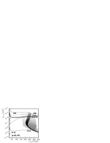
Figure 1: Scatter plots associated with the scalar interaction with non-universal parameters obtained Cerdeno, Gabrielli, Gomez and Munoz. The light grey dotted area corresponds to the laboratory constraints, while the dark dotted area is associated with old relic abundance constraint and the black dotted area with the WMAP relic abundance constraint.

Figure 2: The Total detection rate per $(kg-target)yr$ vs the LSP mass in GeV for a typical solution in our parameter space in the case of ${}^{127}I$. Thick lines correspond to model B, while fine lines to model C. In the upper curve no detector cutoff was employed, while in the lower curve we used a detector energy cutoff of $Q_{min}=10~{}KeV$. Such effects introduce variations in the rates by factors of about two.

To obtain the total rates one must integrate the expressions 14 and 2 over the energy transfer from $Q_{min}$ determined by the detector energy cutoff to $Q_{max}$ determined by the maximum LSP velocity (escape velocity, put in by hand in the Maxwellian distribution), i.e.

$$\upsilon_{esc}=2.84~{}\upsilon_{0}~{}~{},~{}~{}\upsilon_{0}=229~{}Km/s.$$ (22)

In our analysis we included only the rotational velocity of the sun around the center of the galaxy. The local component of the sun‘s velocity is 10 times smaller and it can be neglected.

IV Results

We will specialize the above results in the following cases:

IV.1 Non directional unmodulated rates

Ignoring the motion of the Earth the total non directional rate is given by

$$R=\bar{R}\,t(a,Q_{min})\,~{}~{},~{}~{}\bar{R}=\frac{\rho(0)}{m_{\chi^{0}}}\frac{m}{Am_{p}}~{}(\frac{\mu_{r}}{\mu_{r}(p)})^{2}~{}\sqrt{\langle v^{2}\rangle}[\sigma_{p,\chi^{0}}^{S}~{}A^{2}+\sigma_{p,\chi^{0}}^{spin}~{}\zeta_{spin}]$$ (23)

where $t$ is the ratio of the calculated rate divided by that obtained using the previous equation. It represents the modification of the total rate due to the folding procedure and the nuclear structure effects. $t$ depends on $Q_{min}$, i.e. the energy transfer cutoff imposed by the detector and the parameter $a$ introduced above. All SUSY parameters, except the LSP mass, have been absorbed in $\bar{R}$.

Via Eq. (23) we can, if we wish, extract the nucleon cross section from the data. For most of the allowed parameter space the obtained results for the coherent mode are undetectable in the current experiments. As it has already been mentioned it is possible to obtain detectable rates. Such results have, e.g. recently been obtained by Cerdeno et al CERDENO with non universal set of parameters and the Florida group BAER03 .

A representative set is shown in Fig. 1 or with universal couplings Gomez for large $\tan{\beta}$ in Fig. 2 in the case of the target${}^{127}I$. The planned experiments, like CDMS CDMS , EDELWEISS EDELWEISS , IGEX IGEX , ZEPLIN ZEPLIN and GENIUS GENIUS , are however, expected to improve so that they may detect rates two or three orders of magnitude smaller (see Fig. 1).

In the case of the spin contribution we see that detectable rates are possible only in those cases in which the neutralino has a substantial Higgsino component (see Figs 3- 4 and Figs 5- 6). Our results for the nucleon cross section, obtained by neglecting the isoscalar axial current due to the EMC effect, are in essential agreement with more detailed calculations, which have appeared after our manuscript was completed CCN03 .

Figure 3: The quantity $\bar{R},~{}\approx$ event rate for $Q_{min}=0$, associated with the spin contribution in the case of the $A=19$ system for model n=1 of Chattopadhyay and Roy on the left and model n=75 on the right. The curves from top to bottom correspond to ($sign(\mu),tan(\beta)$) : $(-,40),(+,40),(-,10),(+,10)$. The curves for $\pm 10$ cannot be distinguished from each other.

Figure 4: On the left the same as in Fig. 3 and on the right the proton cross section in $pb$, both for $n=100$. Since the isoscalar contribution is negligible, the neutron cross section is similar.

Figure 5: The quantity $\bar{R},~{}\approx$ event rate for $Q_{min}=0$, associated with the spin contribution in the case of the $A=19$ system for model $M_{1}=(1/3)\mu,M_{2}=(2/3)\mu$ of Murakami and Wells on the left and model $M_{1}=(3/2)\mu,M_{2}=(1/2)\mu$ on the right. The curves are independent of the sign of $\mu$. From top to bottom correspond to $tan(\beta):$ $40,10$.

Figure 6: The same as in Fig. 5 for model $M_{1}=(3/2)\mu,M_{2}=3\mu$ of Murakami and Wells. Note the difference in the scale of the LSP mass compared to Fig. 5.

Figure 7: The event rate, associated with the spin contribution in the case of the $A=127$ system. The notation is the same as in Fig. 3. Only the spherically symmetric velocity distribution ($\lambda=0$) has been considered.

Figure 8: The same as in Fig. 7 for model n=100.

Figure 9: The event rate, associated with the spin contribution in the case of the $A=127$ system for model$M_{1}=(1/3)\mu,M_{2}=(2/3)\mu$ of Murakami and Wells on the left and model $M_{1}=(3/2)\mu,M_{2}=(1/2)\mu$ on the right. The curves are independent of the sign of $\mu$. From top to bottom correspond to $tan(\beta):$ $40,10$.

Figure 10: The same as in Fig. 5 for model $M_{1}=(3/2)\mu,M_{2}=3\mu$ of Murakami and Wells. Note the difference in the scale of the LSP mass compared to Fig. 9.

For the target ${}^{127}I$ the corresponding results are shown in Figs 7- 8 and Figs 9- 10 in the case of the spherically symmetric M.B. velocity distribution and $Q_{min}=0$. The effects of asymmetry and the detector energy cutoff $Q_{min}$ are analogous to those previously found in the coherent mechanism.

IV.2 Modulated Rates

.

If the effects of the motion of the Earth around the sun are included, the total non directional rate is given by

$$R=\bar{R}\,t\,[(1+h(a,Q_{min})cos{\alpha})]$$ (24)

with $h$ the modulation amplitude, relative to the unmodulated (time averaged) amplitude, and $\alpha$ is the phase of the Earth, which is zero around June 2nd. The modulation amplitude would be an excellent signal in discriminating against background, but unfortunately it is very small, less than two per cent (see table 3). Furthermore for intermediate and heavy nuclei, it can even change sign for sufficiently heavy LSP. So in our opinion a better signature is provided by directional experiments, which measure the direction of the recoiling nucleus.

IV.3 Directional Rates.

Since the sun is moving around the galaxy in a directional experiment, i.e. one in which the direction of the recoiling nucleus is observed, one expects a strong correlation of the event rate with the motion of the sun. In fact the directional rate can be written as:

$$R_{dir}=\frac{t_{dir}}{2\pi}\bar{R}\,[1+h_{m}cos{(\alpha-\alpha_{m}~{}\pi)}]=\frac{\kappa}{2\pi}\bar{R}~{}t\,[1+h_{m}cos{(\alpha-\alpha_{m}~{}\pi)}]$$ (25)

where $t_{dir}$ is a quantity analogous to $t$ discussed above, and $h_{m}$ is the modulation. $\alpha_{m}$ is the ”shift” in the phase of the Earth $\alpha$, since now we have both sine and cosine terms and the maximum occurs at $\alpha=\alpha_{m}\pi$. $\kappa/(2\pi)$ is the reduction factor of the unmodulated directional rate relative to the non-directional one. The parameters $\kappa~{},~{}h_{m}~{},~{}\alpha_{m}$ depend on the direction of observation:

$$\hat{e}=(\sin{\Theta}\cos{\Phi}~{},~{}\sin{\Theta}\sin{\Phi}~{},~{}\cos{\Theta})$$

The parameter $t_{dir}$ for a typical LSP mass $100~{}GeV$ is shown in Fig. 11 as a function of the angle $\Theta$ for the targets $A=19$ and $A=127$. We see that the change of the rate as a function of the angle $\Theta$ for the Maxwellian LSP velocity distribution is quite dramatic. This figure is important in the analysis of the angular correlations, since, among other things, there is always un uncertainty in the determination of the angle in a directional experiment.

$t_{dir}\rightarrow$

$\Theta\rightarrow$ $t_{dir}\rightarrow$ $\Theta\rightarrow$

$t_{dir}\rightarrow$

$\Theta\rightarrow$ $t_{dir}\rightarrow$ $\Theta\rightarrow$

Figure 11: The parameter $t_{dir}$ defined in the text as a function of the angle $\Theta$ for $A=19$ at the top and $A=127$ at the bottom. On the left we show $t_{dir}$ for $\lambda=0$ and on the right for $\lambda=1$. The parameter $t_{dir}$ is independent of $\Phi$ for $\lambda=0$ and it depends slightly on it, when $\lambda$ is different from zero. The results presented correspond to an LSP mass of $100~{}GeV$.

$h_{m}\rightarrow$

$\Theta\rightarrow$ $h_{m}\rightarrow$ $\Theta\rightarrow$

$h_{m}\rightarrow$

$\Theta\rightarrow$ $h_{m}\rightarrow$ $\Theta\rightarrow$

$h_{m}\rightarrow$

$\Theta\rightarrow$ $h_{m}\rightarrow$ $\Theta\rightarrow$

Figure 12: The modulation amplitude $h_{m}$ in the case of the $A=19$ system as function of $\Theta$ for $\Phi=0,2\pi$ at the top, $\Phi=\pi/2$ in the middle and $\Phi=3~{}\pi/2$ at the bottom. The values for angles $\Theta\leq 0.5$ should be discarded since the rate is tiny (see Fig. 11). Otherwise the notation is the same as in Fig 11.

$h_{m}\rightarrow$

$\Theta\rightarrow$ $h_{m}\rightarrow$ $\Theta\rightarrow$

$h_{m}\rightarrow$

$\Theta\rightarrow$ $h_{m}\rightarrow$ $\Theta\rightarrow$

$h_{m}\rightarrow$

$\Theta\rightarrow$ $h_{m}\rightarrow$ $\Theta\rightarrow$

Figure 13: The same as in Fig. 12 for A=127.

We sometimes prefer to use the parameters $\kappa=\frac{t_{dir}}{t}$ and $h_{m}$, since, being ratios, are expected to be less dependent on the parameters of the theory. We first exhibit the dependence of $h_{m}$ on the angle $\Theta$ for an LSP mass of $m_{\chi}=100GeV$ in Figs 12 and 13. Then we exhibit the dependence of the parameters $t$, $h$, $\kappa,h_{m}$, and $\alpha_{m}$, which are essentially independent of the LSP mass for target $A=19$, in Table 3 (for the other light systems the results are almost identical).

The asymmetry is quite large. For a Gaussian velocity distribution we find:

$$As=\frac{R(-z)-R(+z)}{R(-z)+R(+z)}\approx 0.97$$

In the other directions it depends on the phase of the Earth and is equal to almost twice the modulation. For a heavier nucleus the situation is a bit complicated. Now the parameters $\kappa$ and $h_{m}$ depend on the LSP mass. The situation is exhibited in Figs 14 and 15. The asymmetry and the shift in the phase of the Earth are similar to those of the $A=19$ system.

$\kappa\rightarrow$

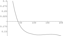
$m_{\chi}\rightarrow$ GeV $\kappa\rightarrow$ $m_{\chi}\rightarrow$ GeV

Figure 14: The parameter $\kappa$ as a function of the LSP mass in the case of the $A=127$ system, associated with the Maxwellian velocity distribution ($\lambda=0$) and $Q_{min}=0$. On the left we show the results for $\Theta=\pi/2$ and on the right $\Theta=\pi$ (the results are independent of $\Phi$). The rate for $\Theta=0$ is negligible.

$h_{m}\rightarrow$

$m_{\chi}\rightarrow$ GeV $h_{m}\rightarrow$ $m_{\chi}\rightarrow$ GeV

$h_{m}\rightarrow$

$m_{\chi}\rightarrow$ GeV $h_{m}\rightarrow$ $m_{\chi}\rightarrow$ GeV

Figure 15: The modulation amplitude $h_{m}$. From left to right and top to bottom the graphs correspond to $\pm x,+y,-y,-z$. Otherwise the notation is the same as in Fig 14.

In the results shown we only considered the rotational velocity of the sun around the center of the galaxy. We do not, however, expect a significant modification, if the other components of the sun‘s velocity, which are an order of magnitude smaller, are included.

V Conclusions

It is well known that, in the coherent case, only in a small segment of the allowed parameter space the rates are above the present experimental goals  Gomez ; ref2 ; ARNDU , which of course may be improved by two or three orders of magnitude in the planned experiments CDMS -GENIUS . In the case of the spin contribution only in models with large higgsino components of the LSP one can obtain rates, which may be presently detectable, but in this case, except in special models, the bound on the relic LSP abundance may be difficult to respect. Anyway it appears that in both cases the expected rates are small. It may, therefore, be necessary to exploit any characteristic experimental signatures, which may reduce the formidable backgrounds at such low counting rates.

In the present paper we considered the spin induced rates and examined the following signatures:

• Correlation of the event rates with the motion of the Earth (modulation effect)

• Angular correlation of the directional rates with the direction of motion of the sun as well as their seasonal variation.
  Such experiments are currently under way, like the UKDMC DRIFT PROJECT experiment UKDMC , the Micro-TPC Detector of the Kyoto-Tokyo collaboration KYOTOK and the TOKYO experiment TOKYO .

Let us first consider the conventional experiments and focus on the relative parameters $t=R/\bar{R}$ and the modulation (seasonal variation) amplitude $h$, normalized to zero when the motion of the Earth is ignored. In the case of light nuclear targets they are essentially independent of the LSP mass, but they depend on the energy cutoff, $Q_{min}$. For $Q_{min}=0$ they are exhibited in Table 3. They are essentially the same for both the coherent and the spin modes. For intermediate and heavy nuclei they depend on the LSP mass JDV03 . It is clear that among the light targets, from the point of view of the static spin matrix elements, the most favored system DIVA00 is the $A=19$, since the spin matrix elements are both large and very reliably calculated. We should keep in mind, however, that for heavy LSP the reduced mass can be large in the case of a heavy nucleus like ${}^{207}Pb$. The increase of the rates caused by the increase of the reduced mass may very well compensate for the smallness of the spin matrix elements. As a matter of fact in the case of ${}^{127}I$ we see that, for an LSP mass greater than $100~{}GeV$, the obtained rate is larger than that of ${}^{19}F$ in spite of the fact that the dominant isovector static spin matrix elements are in the opposite order. We should not forget, though, that the calculated spin matrix elements in the case of the $A=19$ system are more reliable.

In the case of the directional experiments, i.e when only nuclei recoiling in a certain direction are counted, we can summarize our results as follows:

• The angular dependence of the rate.
  The ratio of the directional rate divided by that of the usual rate , given by $\approx\kappa/(2\pi)$, is smaller than $1/5\pi$. Such a big loss in the rate may very well be compensated by the important experimental signature associated with the fact that the factors $\kappa$ depend on the direction of observation. In the case of a Gaussian velocity distribution this factor is the largest, $\kappa\approx 0.4$, when the nucleus is recoiling opposite to the direction of motion of the sun. $\kappa$ is the smallest in the direction of the sun’s motion (least favored direction) and in between for the other directions. In other words the directional rate is strongly peaked in the direction opposite to the velocity of the sun and the resulting event asymmetry between these two directions is very large. In a plane perpendicular to the sun’s direction of motion $\kappa$ takes intermediate values, $\kappa\approx 0.08$. The asymmetry between one direction and its opposite is in this case almost zero, if the motion of the Earth is neglected. Anyway the study of such angular correlations may play a role in confirming any observed neutralino events, since there may appear seasonal effects, which can mimic the small modulation in the conventional experiments.

• Seasonal variation (modulation) of the directional rates.
  We have shown that the directional rates can, in addition, exhibit seasonal variation (modulation). In the most favored direction the modulation is not very large, but still it is three times larger compared to that expected in the standard non directional experiments. This gain is , perhaps, not big enough to compensate for the reduction in the number of the events. In a plane perpendicular to the sun’s direction of motion, however, the modulation is quite large (see Table 3). The experimentalists will themselves decide what use, if any, to make of these predictions. A simple argument indicates that they may be useful. Taking, as an example, events in the x-direction (radial galactic direction), we can see that the modulation signal will be reduced by a factor of $(2\pi/0.08)(0.272/0.02)=5.8$ The background will be reduced by a factor of $\sqrt{(2\pi/0.08)}=8.9$. Thus one expects a gain of $1.5$.
  Furthermore the modulation in this plane is characterized by a very interesting seasonal pattern, depending on the angle of observation (see Table 3). Perhaps this also can be exploited by the experimentalists.

The predicted reductions in the rates of the directional experiments compared to the standard experiments, at a first sight, may be seen as an obstacle to be overcome for the benefit of the above good signatures. This may be true in the case of some of the planned experiments TOKYO , which intend to use organic detectors capable of making observations in only one predetermined direction for each run. Quite clearly, however, the directional observations are going to offer only advantages in the case of experiments using TPC detectors UKDMC ; KYOTOK . The TPC counters can simultaneously register all events. If something interesting is found, the analysis can be made directionally to reject possible background events.

We finally hope that, in spite of the reduction in the predicted rates, the signatures of the directional experiments (large asymmetry and modulation amplitude) can be exploited by the experimentalists.

Acknowledgments: This work was supported in part by the European Union under the contracts RTN No HPRN-CT-2000-00148 and TMR No. ERBFMRX–CT96–0090. Part of this work was performed in LANL. The author is indebted to Dr Dan Strottman for his support and hospitality and to Hiro Ejiri for his useful comments on the preparation of the manuscript. He is also grateful to Y. Giomataris and K. Zioutas for bringing to his attention the great opportunities offered by the TPC detectors.

Table 1: A summary of the parameters $C^{n}_{i}$ of the model of Chattopadhyay and Roy and the relevant renormalization factors.

n/i	3	2	1	comment
1	1	1	1	SUGRA (Bino)
24	1	-3/2	-1/2	Bino
75	1	3	-5	Zino
100	1	2	10	Higgsino
	25/9	25/30	25/60	Ren. factor

Table 2: The static spin matrix elements for various nuclei. For light nuclei the calculations are from Divari et al (see text) . For ${}^{127}I$ the results are from Ressel and Dean (see text) (*) and the Jyvaskyla-Ioannina collaboration (private communication)(**). For ${}^{207}Pb$ they were obtained previously (see text).

	19F	29Si	23Na	${}^{127}I^{*}$	${}^{127}I^{**}$	${}^{207}Pb^{+}$
$[\Omega_{0}(0)]^{2}$	2.610	0.207	0.477	3.293	1.488	0.305
$[\Omega_{1}(0)]^{2}$	2.807	0.219	0.346	1.220	1.513	0.231
$\Omega_{0}(0)\Omega_{1}(0)$	2.707	-0.213	0.406	2.008	1.501	-0.266
$\mu_{th}$	2.91	-0.50	2.22
$\mu_{exp}$	2.62	-0.56	2.22
$\frac{\mu_{th}(spin)}{\mu_{exp}}$	0.91	0.99	0.57

Table 3: The parameters $t$, $h$, $\kappa,h_{m}$ and $\alpha_{m}$ for the isotropic Gaussian velocity distribution and $Q_{min}=0$. The results presented are associated with the spin contribution, but those for the coherent mode are similar. The results shown are for the light systems. For intermediate and heavy nuclei there is a dependence on the LSP mass. $+x$ is radially out of the galaxy ($\Theta=\pi/2,\Phi=0$), $+z$ is in the sun’s direction of motion ($\Theta=0$) and $+y$ is vertical to the plane of the galaxy ($\Theta=\pi/2,\Phi=\pi/2$) so that $(x,y,z)$ is right-handed. $\alpha_{m}=0,1/2,1,3/2$ means that the maximum occurs on the 2nd of June, September, December and March respectively.

type	t	h	dir	$\kappa$	$h_{m}$	$\alpha_{m}$
			+z	0.0068	0.227	1
dir			+(-)x	0.080	0.272	3/2(1)
			+(-)y	0.080	0.210	0 (1)
			-z	0.395	0.060	0
all	1.00
all		0.02

References

-
(1)
S. Hanary et al, Astrophys. J. 545, L5 (2000);
J.H.P Wu et al, Phys. Rev. Lett. 87, 251303 (2001);
M.G. Santos et al, Phys. Rev. Lett. 88, 241302 (2002) -
(2)
P.D. Mauskopf et al, Astrophys. J. 536, L59 (20002);
S. Mosi et al, Prog. Nuc.Part. Phys. 48, 243 (2002);
S.B. Ruhl al, astro-ph/0212229 and references therein. -
(3)
N.W. Halverson et al, Astrophys. J. 568, 38 (2002)
L.S. Sievers et al,astro-ph/0205287 and references therein. - (4) G.F. Smoot et al, (COBE data), Astrophys. J. 396, (1992) L1.
- (5) A.H. Jaffe et al.,Phys. Rev. Lett. 86, 3475 (2001).
- (6) D.N. Spergel et al,Astrophys. J. Suppl. 148, 175 (2003); astro-ph/0302209
- (7) M. Tegmark et al, Cosmological parameters from SDSS and WMAP, astro-ph/0310723
-
(8)
D.P. Bennett et al., (MACHO collaboration), A binary
lensing event toward the LMC: Observations and Dark Matter
Implications,
Proc. 5th Annual Maryland Conference, edited by S. Holt (1995);
C. Alcock et al., (MACHO collaboration), Phys. Rev. Lett. 74 , 2967 (1995). - (9) R. Bernabei et al., INFN/AE-98/34, (1998); R. Bernabei et al., it Phys. Lett. B 389, 757 (1996).
- (10) R. Bernabei et al., Phys. Lett. B 424, 195 (1998); B 450, 448 (1999).
-
(11)
For a review see:
G. Jungman, M. Kamionkowski and K. Griest , Phys. Rep. 267 (1996) 195. - (12) M.W. Goodman and E. Witten, Phys. Rev. D 31, 3059 (1985).
- (13) K. Griest, Phys. Rev. Lett 61, 666 (1988).
- (14) J. Ellis, and R.A. Flores, Phys. Lett. B 263, 259 (1991); Phys. Lett. B 300, 175 (1993); Nucl. Phys. B 400, 25 (1993).
- (15) J. Ellis and L. Roszkowski, Phys. Lett. B 283, 252 (1992).
-
(16)
For more references see e.g. our previous report:
J.D. Vergados, Supersymmetric Dark Matter Detection- The Directional Rate and the Modulation Effect, hep-ph/0010151; -
(17)
M.E.Gómez and J.D. Vergados, Phys. Lett. B 512
, 252 (2001); hep-ph/0012020.
M.E. Gómez, G. Lazarides and Pallis, C., Phys. Rev.D 61 123512 (2000) and Phys. Lett. B 487, 313 (2000). - (18) M.E. Gómez and J.D. Vergados, hep-ph/0105115.
-
(19)
A. Bottino et al., Phys. Lett B 402, 113 (1997).
R. Arnowitt. and P. Nath, Phys. Rev. Lett. 74, 4952 (1995); Phys. Rev. D 54, 2394 (1996); hep-ph/9902237;
V.A. Bednyakov, H.V. Klapdor-Kleingrothaus and S.G. Kovalenko, Phys. Lett. B 329, 5 (1994). - (20) U. Chattopadhyay, A. Corsetti and P. Nath, Phys. Rev. D 68, 035005 (2003).
- (21) U. Chattopadhyay and D.P. Roy, Phys. Rev. D 68, 033010 (2003); hep-ph/0304108.
- (22) B. Murakami and J.D. Wells, Phys. Rev. D 64 (2001) 015001;hep-ph/0011082
- (23) J.D. Vergados, J. of Phys. G 22, 253 (1996).
- (24) A. Arnowitt and B. Dutta, Supersymmetry and Dark Matter, hep-ph/0204187.
- (25) E. Accomando, A. Arnowitt and B. Dutta, Dark Matter, muon G-2 and other accelerator constraints, hep-ph/0211417.
- (26) T.S. Kosmas and J.D. Vergados, Phys. Rev. D 55, 1752 (1997).
- (27) M. Drees and N,M. Nojiri, Phys. Rev. 471993376; (1985).
- (28) M. Drees and N.N. Nojiri, Phys. Rev. D 48, 3843 (1993); Phys. Rev. D 47, 4226 (1993).
- (29) A. Djouadi and MK. Drees, Phys. Lett. B 484, 183 (2000); S. Dawson, Nucl. Phys. B359, 283 (1991); M. Spira it et al, Nucl. Phys. B453, 17 (1995).
- (30) T.P. Cheng, Phys. Rev. D 38, 2869 (1988); H-Y. Cheng, Phys. Lett. B 219, 347 (1989).
- (31) M.T. Ressell et al., Phys. Rev. D 48, 5519 (1993); M.T. Ressell and D.J. Dean, Phys. Rev. C bf 56 (1997) 535.
- (32) J.D. Vergados and T.S. Kosmas, Physics of Atomic nuclei, Vol. 61, No 7, 1066 (1998) (from Yadernaya Fisika, Vol. 61, No 7, 1166 (1998).
- (33) P.C. Divari, T.S. Kosmas, J.D. Vergados and L.D. Skouras, Phys. Rev. C 61 (2000), 044612-1.
- (34) A.K. Drukier, K. Freese and D.N. Spergel, Phys. Rev. D 33, 3495 (1986).
- (35) K. Frese, J.A Friedman, and A. Gould, Phys. Rev. D 37, 3388 (1988).
- (36) J.D. Vergados, Phys. Rev. D 58, 103001-1 (1998).
- (37) J.D. Vergados, Phys. Rev. Lett. 83, 3597 (1999).
- (38) J.D. Vergados, Phys. Rev. D 62, 023519 (2000).
- (39) J.D. Vergados, Phys. Rev. D 63, 06351 (2001).
- (40) J.I. Collar et al, Phys. Lett. B 275, 181 (1992).
- (41) P. Ullio and M. Kamioknowski, JHEP 0103, 049 (2001).
- (42) P. Belli, R. Cerulli, N. Fornego and S. Scopel, P͡hys. Rev. D 66, 043503 (2002); hep-ph/0203242.
- (43) A. Green, Phys. Rev. D 66, 083003 (2002)
- (44) K.N. Buckland, M.J. Lehner and G.E. Masek, in Proc. 3nd Int. Conf. on Dark Matter in Astro- and part. Phys. (Dark2000), Ed. H.V. Klapdor-Kleingrothaus, Springer Verlag (2000).
- (45) A. Brignole, L.E. Ibanez and C. Munoz, Nuc. Phys. 422 (1994) 125.
- (46) J. Ellis, A. Ferstl and K.A. Olive, Phys. Lett B 481 (2000) 304 .
- (47) A. Bottino, F. Donnato, N. Fornengo, and S. Scopel, hep-ph/0111229.
- (48) M. Gomez, T. Gutsche and J.D. Vergados, to be published.
- (49) D.G. Cerdeno, E. Gabrielli, M.E. Gomez and C. Munoz, hep-ph/0304115
- (50) H. Baer, C. Balazs, A. Belyaev and J. O’ Farrill, hep-ph/0305191D
- (51) CDMS Collaboration, R. Abusaidi et al, Phys. Rev. Lett. 84 (2000) 56599; Phys. Rev D 66 (2002) 122003.
- (52) EDELWEISS Collaboration, A. Bennoit et al, Phys. Lett. B 513 (2001) 15; ibid B 545 (2002) 23.
- (53) IGEX Collaboration, A. Morales et al, Phys. Lett. B 532 (2002) 8.
- (54) ZEPLIN I Collaboration, N.J.T. Smith et al, talk given at the 4th International Workshop on Identification of Dark Matter, IDM2002, York, U.K.
-
(55)
GENIUS Collaboration, H.V. Klapdor-Kleingrothauset al, Proceedings of
DARK2000, Ed. H.V. Klapdor-Kleingrothaus, Springer Berlin (2000);
hep-ph/0103062
GENIUS Collaboration, H.V. Klapdor-Kleingrothauset al, Nuc. Phys. Proc. Suppl. 110 (2002) 364; hep-ph/0206249. - (56) J.D. Vergados, Phys. Rev. D 67 (2003) 103003.
- (57) A. Takeda et al, First Yamada Symposium on Neutrinos and Dark Matter in Nuclear Physics (NDM03), Nara, Japan, June 9-14, 2003 ( to appear in the proceedings).
- (58) A. Shimizu et al, First Yamada Symposium on Neutrinos and Dark Matter in Nuclear Physics (NDM03), Nara, Japan, June 9-14, 2003 ( to appear in the proceedings); astro-ph/0207529