Large Logarithms in the Beam Normal Spin Asymmetry
of Elastic Electron–Proton Scattering

Abstract

We study a parity-conserving single-spin beam asymmetry of elastic electron-proton scattering induced by an absorptive part of the two-photon exchange amplitude. It is demonstrated that excitation of inelastic hadronic intermediate states by the consecutive exchange of two photons leads to logarithmic and double-logarithmic enhancement due to contributions of hard collinear quasi-real photons. The asymmetry at small electron scattering angles is expressed in terms of the total photoproduction cross section on the proton, and is predicted to reach the magnitude of 20-30 parts per million. At these conditions and fixed 4-momentum transfers, the asymmetry is rising logarithmically with increasing electron beam energy, following the high-energy diffractive behavior of total photoproduction cross section on the proton.

I Introduction

Recently the two–photon exchange (TPE) mechanism in elastic electron–proton scattering started to draw a lot of attention. The reason is that this mechanism possibly accounts for the difference between the high–$Q^{2}$ values of the ratio $G_{Ep}/G_{Mp}$ Mel measured in unpolarized and polarized electron scattering. Calculations of Ref.Afanas using a formalism of Generalized Parton Distributions GPD confirm such a possibility and decisive experimental tests are being proposed Brooks .

On the other hand, it has been known for a long time ST1 ; Barut ; Ru that the TPE mechanism can generate the single-spin normal asymmetry (SSNA) of electron scattering due to a nonzero imaginary ($\Im$) part of the TPE amplitude $A_{2\gamma}$,

$$A_{n}=\frac{2A_{Born}\Im(A^{*}_{2\gamma})}{|A_{Born}|^{2}}\,$$ (1)

where the one-photon-exchange amplitude $A_{Born}$ is purely real due to time-reversal invariance of electromagnetic interactions.

Our earlier calculations of the TPE effect on the proton aam predicted the magnitude of beam SSNA at the level of a few parts per million (ppm). The effect appears to be small due to two suppression factors combined: $\alpha=1/137$, since the effect is higher-order in the electromagnetic interaction; and a factor of electron mass $m_{e}$ arising due to electron helicity flip. The predictions of Ref.aam , assuming no inelastic excitations of the intermediate proton, used only proton elastic form factors as input parameters and appeared to be in qualitative agreement with experimental data from MIT/Bates Wells . The result of Ref.aam with an elastic intermediate proton state was reproduced later in Ref.Mark . In another calculation of beam SSNA of Ref.Musolf , a low-momentum expansion was used for the TPE loop integral, which resulted in approximate analytic expressions valid for low electron beam energies. The main theoretical problem in description of the TPE amplitude on the proton at higher energies in the GeV range is a large uncertainty in the contribution of the inelastic hadronic intermediate states. In Ref.Mark the beam SSNA at large momentum transfers was estimated at the level of one ppm, using the partonic framework developed in Ref.Afanas for TPE effects not related to the electron helicity flip.

Current experiments designed for parity-violating electron scattering allow to measure the beam asymmetry with a fraction of ppm accuracy Maas ; E158 ; PViol and may also provide data on the parity-conserving beam SSNA. In fact, such measurements are needed because beam SSNA is a source of systematic corrections in the measurements of parity-violating observables.

During our previous work aam we noticed that while considering excitation of inelastic intermediate hadronic states, the expressions for the beam SSNA (Eq.(11) of Ref.aam ), after factoring out the electron mass, have an enhancement when at least one of the photons in the TPE loop integral is collinear to its parent electron, i.e. the virtuality of the exchanged photon is of the order of electron mass. It is interesting that this effect did not appear for the target SSNA calculations aam . Independently, enhancement due to exchange of collinear photons for the beam SSNA was observed by other authors Ref.Pasquini , who considered the hadronic intermediate states in the TPE amplitude in the nucleon resonance region using a phenomenological model (MAID) for single–pion electroproduction.

In this paper, we study the analytic structure of the collinear-photon exchange in the TPE amplitude and demonstrate that it results in enhancement of the beam SSNA described by single and double logarithms of the type $\log(Q^{2}/m_{e}^{2})$ and $\log^{2}(Q^{2}/m_{e}^{2})$. Using a general requirement of gauge invariance of the nonforward nucleon Compton tensor, we find that such enhancement does not take place for the target SSNA (with unpolarized electrons) and spin correlations caused by longitudinal polarization of the scattering electrons. When modelling the TPE mechanism with nucleon resonance excitation, we observe that depending on the electron beam energy, the beam SSNA has a double-logarithmic enhancement if the Mandelstam variable $\sqrt{s}$ nears the resonance mass, and a single-logarithmic enhancement otherwise. For electron energies above the resonance region and small scattering angles, we use an optical theorem to relate the nucleon Compton amplitude to the total photoproduction cross section and obtain a simple analytic formula for the beam SSNA in this kinematics.

II Properties of leptonic tensor

First, we write the formula for SSNA in terms of rank-3 leptonic and hadronic tensors which appear in the interference between the Born and TPE amplitudes as shown in Fig.1.

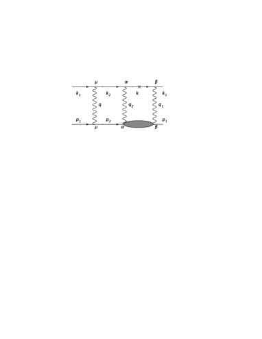
Figure 1: Interference between the Born and the TPE box diagrams in elastic e-p scattering that determined SSNA.

$$A_{n}=\frac{-i\alpha Q^{2}}{\pi^{2}D(s,Q^{2})}\int\frac{d^{3}k}{2E_{k}}\frac{L_{\mu\alpha\beta}H_{\mu\alpha\beta}}{q_{1}^{2}q_{2}^{2}}\ ,$$ (2)

where $Q^{2}=-q^{2}$, $k(E_{k})$ is the 3-momentum (energy) of the intermediate on-mass-shell electron in the TPE box diagram, $q_{1}$ and $q_{2}$ are the 4-momenta of the intermediate photons, $q_{1}-q_{2}=q$. The factor $Q^{2}/D(s,Q^{2})$ in Eq.(2) is due to the squared Born amplitude, namely,

$$D(s,Q^{2})=\frac{Q^{4}}{2}\big{(}F_{1}+F_{2}\big{)}^{2}+[(s-M^{2})^{2}-$$ (3)

$$Q^{2}s]\Big{(}F_{1}^{2}+\frac{Q^{2}}{4M^{2}}F_{2}^{2}\Big{)},$$

where $F_{1}(F_{2})$ is the Dirac (Pauli) proton form factor, $M$ is the proton mass and $s=(k_{1}+p_{1})^{2}$ is a Mandelstam variable. Our sign convention for the beam asymmetry follows from the definition of the normal vector with respect to the electron scattering plane: ${\bf{k}_{1}}\times{\bf{k}_{2}}.$

Using the above notation, we have

$$L_{\mu\alpha\beta}=\frac{1}{4}Tr(\hat{k}_{2}+m_{e})\gamma_{\mu}(\hat{k}_{1}+m_{e})(1-\gamma_{5}\hat{\xi^{e}})\gamma_{\beta}(\hat{k}+m_{e})\gamma_{\alpha}\ ,$$ (4)

and

$$H_{\mu\alpha\beta}=\frac{1}{4}Tr(\hat{p}_{2}+M)\Gamma_{\mu}(\hat{p}_{1}+M)(1-\gamma_{5}\hat{\xi^{p}})\Im T_{\beta\alpha}\ ,$$ (5)

where $m_{e}$ is the electron mass, $\xi^{e}(\xi^{p})$ is the polarization 4-vector of the electron beam (proton target), $\Gamma_{\mu}=\gamma_{\mu}(F_{1}+F_{2})-(p_{1\mu}+p_{2\mu})F_{2}/(2M)$, and $T_{\beta\alpha}$ is in general a non-forward proton Compton tensor that describes any possible hadronic intermediate states in the TPE amplitude, while the symbol $\Im$ denotes the imaginary (absorptive) part. Thus, we see that in accordance with Eq.(2) the single-spin normal asymmetry probes the imaginary part of contraction of the leptonic and hadronic tensors defined by Eqs.(4) and (5), respectively. In turn, this imaginary part is related with the imaginary part of the nucleon non-forward Compton tensor $\Im T_{\beta\alpha}$. It was noted by De Rujula et al. Ru awhile ago for the case of normal polarization of the proton target. For the case of beam SSNA on a proton, the first calculation was done in Ref.aam .

After some algebra we arrive at the following expression for the model-independent leptonic tensor

$$L_{\mu\alpha\beta}=L^{(un)}_{\mu\alpha\beta}+L^{(pol)}_{\mu\alpha\beta}\ ,$$ (6)

where the spin–independent part is

$$L^{(un)}_{\mu\alpha\beta}=\frac{1}{2}q_{1}^{2}(g_{\mu\beta}k_{2\alpha}-g_{\mu\alpha}k_{2\beta})-\frac{1}{2}q_{2}^{2}(g_{\mu\beta}k_{1\alpha}-g_{\mu\alpha}k_{1\beta})-$$

$$k_{\mu}[k_{1}k_{2}]_{\alpha\beta}+\frac{1}{2}g_{\alpha\beta}(q_{1}^{2}k_{2\mu}+q_{2}^{2}k_{1\mu}-q^{2}k_{\mu})+$$ (7)

$$\frac{1}{2}q^{2}(g_{\mu\alpha}k_{\beta}+g_{\mu\beta}k_{\alpha})+k_{2\mu}(kk_{1})_{\alpha\beta}+k_{1\mu}(kk_{2})_{\alpha\beta}\ ,$$

$$[ab]_{\alpha\beta}=a_{\alpha}b_{\beta}-a_{\beta}b_{\alpha}\ ,\ \ (ab)_{\alpha\beta}=a_{\alpha}b_{\beta}+a_{\beta}b_{\alpha}\ ,$$

and the spin–dependent part is given by

$$L^{(pol)}_{\mu\alpha\beta}=im_{e}\bigg{[}-g_{\alpha\beta}(\mu qq_{2}\xi^{e})+k_{\beta}(\mu\alpha q\xi^{e})+k_{\alpha}(\mu\beta q\xi^{e})$$

$$+\xi^{e}_{\mu}(\alpha\beta qq_{2})+(\xi^{e}k_{2})(\mu\alpha\beta q_{1})+k_{2\mu}(\alpha\beta q_{1}\xi^{e})+$$ (8)

$$k_{1\mu}(\alpha\beta q_{2}\xi^{e})+\frac{1}{2}q^{2}(\mu\alpha\beta\xi^{e})\bigg{]}\ ,$$

$$(abcd)\equiv\epsilon_{\nu\lambda\rho\sigma}a_{\nu}b_{\lambda}c_{\rho}d_{\sigma}\ ,$$

where the on-shell condition $k^{2}_{\mu}=m_{e}^{2}$ was used for the intermediate electron 4-momentum. The above leptonic and hadronic tensors satisfy the conditions

$$L_{\mu\alpha\beta}q_{\mu}=L_{\mu\alpha\beta}q_{2\alpha}=L_{\mu\alpha\beta}q_{1\beta}=0$$

$$H_{\mu\alpha\beta}q_{\mu}=H_{\mu\alpha\beta}q_{2\alpha}=H_{\mu\alpha\beta}q_{1\beta}=0$$ (9)

separately for spin–independent and spin–dependent parts, as follows from gauge invariance of electromagnetic interactions.

Let us consider the leptonic tensor in the limiting case when one of the intermediate photon in the box diagram is collinear to its parent electron, for example, when $q_{1}=xk_{1},\ x\simeq 1.$ Note first that for elastic proton intermediate state such kinematics is not allowed by the 4-momentum conservation, $(xk_{1}+p_{1})^{2}=M^{2}$. But for the inelastic intermediate excitations we have $x=(W^{2}-M^{2})/(s-M^{2}),$ where $W^{2}$ is the squared invariant mass of the intermediate hadronic system.

It can be seen, using the relations

$$q_{2}^{2}=(1-x)q^{2},\ \ k=(1-x)k_{1},\ \ q_{1}^{2}\simeq 0$$ (10)

that in the considered conditions the unpolarized leptonic tensor is given by

$$L^{(un)}_{\mu\alpha\beta}=\frac{1-x}{x}q_{1\beta}\Big{[}q^{2}g_{\mu\alpha}+2(k_{1}k_{2})_{\mu\alpha}\Big{]}\ .$$ (11)

Because any gauge-invariant hadronic tensor has to give zero after contracting with $q_{1\beta}$ (see Eq.(9)), we conclude that collinear photon kinematics does not contribute to the target SSNA (or recoil proton polarization) which are defined by the spin–independent part of the leptonic tensor $L_{\mu\alpha\beta}.$ This conclusion confirms our previous calculations aam .

For the spin–dependent part of leptonic tensor, we obtain in the considered limit,

$$\frac{1}{im_{e}}L^{(pol)}_{\mu\alpha\beta}\Big{|}_{q_{1}\to xk_{1}}=\frac{2(1-x)}{x}q_{1\beta}(\mu\alpha q\xi^{e})+$$

$$x\Big{[}-g_{\alpha\beta}(\mu qk_{1}\xi^{e})+\frac{q^{2}}{2}(\mu\alpha\beta\xi^{e})+\xi^{e}_{\mu}(\alpha\beta qk_{1})+$$ (12)

$$(\xi^{e}k_{2})(\mu\alpha\beta k_{1})+k_{2\mu}(\alpha\beta k_{1}\xi^{e})+k_{1\mu}(\alpha\beta k_{2}\xi^{e})\Big{]}\ .$$

If the electron beam is polarized longitudinally, ($\xi^{e}_{\mu}\simeq k_{1\mu}/m_{e}$), the term in the square brackets of Eq.(12) turns to zero, and we have the same situation as in the case of unpolarized beam, namely, the region of the small $q_{1}^{2}$ (or $q_{2}^{2}$) does not contribute when the intermediate photon is collinear to its parent electron.

A different phenomenon takes place in the case of the normal polarized electron beam

$$\xi^{e}_{\mu}=\frac{2(\mu k_{1}p_{1}q)}{\sqrt{Q^{2}[(s-M^{2})^{2}-Q^{2}s]}}\ .$$ (13)

In this case the term in square brackets of Eq.(12) is not zero and the considered collinear photon kinematics contributes with essential logarithmic enhancement. Moreover, here we will demonstrate using specific examples that this enhancement can be double-logarithmic.

Therefore, conservation of the electromagnetic current that follows from gauge invariance (Eq.(9)) is the reason why the collinear intermediate photons appear in the TPE contribution to the beam SSNA, but not to the target SSNA. By analogy, we do not anticipate contributions from collinear-photon exchange in unpolarized electron-proton scattering, parity-violating asymmetries due to longitudinal electron polarization, charged current neutrino-nucleon scattering and/or lepton weak capture if the normal polarization of leptons is not involved.

III Hadronic tensor in the resonance region

We first study the analytic properties TPE loop integration in a resonance model taking into account nucleon resonances with quantum numbers $N^{*}\Big{(}\frac{1^{+}}{2}\Big{)},\ N^{*}\Big{(}\frac{1^{-}}{2}\Big{)}$ and $\Delta\Big{(}\frac{3^{+}}{2}\Big{)}$ as intermediate hadronic states. In this model the imaginary part of the nucleon Compton tensor is given by

$$\Im T_{\beta\alpha}=\Im\Big{[}T_{\beta\alpha}(+)+T_{\beta\alpha}(-)+T_{\beta\alpha}(\Delta)\Big{]}\ .$$ (14)

Using a general Lorentz structure of nucleon resonance excitations, we verified that the contribution from collinear kinematics of intermediate photons is zero for the quantity $L_{\mu\alpha\beta}H_{\mu\alpha\beta}$ (Eq.(2)) for the unpolarized electron beam. On the contrary, if the electron beam has normal polarization, the resulting expression is proportional to the difference between the resonance and the proton masses. Thus, we conclude that the collinear intermediate photons can give a large contribution to the beam SSNA in the resonance region.

For example, the general form of the integrand $L_{\mu\alpha\beta}H_{\mu\alpha\beta}$ in the case of intermediate Roper $N\Big{(}\frac{1^{+}}{2}\Big{)}$ resonance excitation is proportional to

$$\Big{(}a+bq_{1}^{2}+cq_{2}^{2}+dq_{1}^{2}q_{2}^{2}+eq_{1}^{4}+fq_{2}^{4}\Big{)}F_{R}(q_{1}^{2})F_{R}(q_{2}^{2})\ ,$$ (15)

where coefficients $a,\ b,...$ depend on $M,\ M_{R},\ s$ and $q^{2}$ and $F_{R}(q_{1,2}^{2})$ are the transition form factors of the resonance excitation.

The 3-dimensional loop integration in Eq.(2) is done over all allowed angles of the intermediate electron and the invariant mass of the intermediate hadronic state in the range $M+m_{\pi}<W<\sqrt{s}-m_{e}$, as follows from the energy-momentum conservation, where $W^{2}=(q_{1}+p_{1})^{2}=(q_{2}+p_{2})^{2}$ and $m_{\pi}$ is a pion mass. Namely,

$$\frac{d^{3}k}{2E_{k}}=\frac{k\ dW^{2}}{4\sqrt{s}}d\Omega_{k}\ .$$

In the c.m.s.

$$q_{1}^{2}=2m_{e}^{2}+2kk_{1}\cos{\theta_{1}}-2E_{k}E_{k1},$$

$$q_{2}^{2}=2m_{e}^{2}+2kk_{1}\cos{\theta_{2}}-2E_{k}E_{k1},$$ (16)

where $k_{1}$ and $E_{k1}$ are the 3-momentum and the energy of the initial electron, $\theta_{1}(\theta_{2})$ is the angle between 3-momenta of the intermediate and the initial (scattered) electrons.

Collinear photon kinematics corresponds to $\cos{\theta_{1}}\simeq 1$ (or $\cos{\theta_{2}}\simeq 1$ when the quantities $q_{1}^{2}$ and $q_{2}^{2}$ become small and change from their minimal value $(2m_{e}^{2}+2kk_{1}-2E_{k}E_{k1})$ up to $E_{k}E_{k1}\theta_{1}^{2}.$ The most singular term in the TPE diagram integral at such conditions comes from the coefficient $a$ in Eq.(15). We use a substraction procedure to present the result of angular integration of this term,

$$\int\frac{d\Omega_{k}}{q_{1}^{2}q_{2}^{2}}F_{R}(q_{1}^{2})F_{R}(q_{2}^{2})=\int\frac{d\Omega_{k}}{q_{1}^{2}q_{2}^{2}}\Phi_{0}(q_{1}^{2},q_{2}^{2})-$$

$$\frac{2\pi}{E_{k1}k}\int\limits_{-1}^{1}\frac{dc_{1}}{|c-c_{1}|}\Big{[}\frac{\Phi_{1}(q_{1}^{2})}{q_{1}^{2}}-\frac{\Phi_{1}(q_{1c}^{2})}{q_{1c}^{2}}\Big{]}-$$

$$\frac{2\pi}{q_{1c}^{2}E_{k1}k}\Phi_{1}(q_{1c}^{2})L_{2}+\frac{\pi}{Q^{2}k^{2}}F^{2}_{R}(0)L_{1}\ ,$$ (17)

where $c=\cos{\theta}$, with $\theta$ being the electron c.m.s. scattering angle, $c_{1}=\cos{\theta_{1}}$, $q^{2}_{1c}=q_{1}^{2}(c_{1}\rightarrow c)$ and

$$\Phi_{0}(q_{1}^{2},q_{2}^{2})=F_{R}(q_{1}^{2})F_{R}(q_{2}^{2})-F_{R}(0)[F_{R}(q_{1}^{2})+F_{R}(q_{2}^{2})]+$$

$$F^{2}_{R}(0),\ \ \ \Phi_{1}(q_{1}^{2})=F_{R}(0)[F_{R}(q_{1}^{2})-F_{R}(0)]\ ,$$

$$L_{1}=\frac{1}{K}\log\frac{2K+1}{2K-1},\ \ K=\sqrt{\frac{1}{4}+\eta},\ \ \eta=\frac{m_{e}^{2}(E_{k1}-E_{k})^{2}}{Q^{2}k^{2}}\ ,$$

$$L_{2}=\log\frac{A_{+}A_{-}}{m_{e}^{2}(E_{k1}-E_{k})^{2}\sin^{2}{\theta}}\ ,\ A_{\pm}=k_{1}k\pm E_{k1}E_{k}c$$

$$+\sqrt{(k_{1}k\pm E_{k1}E_{k}c)^{2}+m_{e}^{2}\sin^{2}{\theta}(E_{k1}-E_{k})^{2}}.$$ (18)

The first two terms in the r.h.s. of Eq.(17) are regular and they can be easily integrated numerically (after choosing specific parametrization of $F_{R}(q_{1}^{2})$), whereas the last two ones, enhanced logarithmically, appear due to proximity to the dynamical pole that arises from collinear photon kinematics, and increased precision is required if this problem were solved entirely by numerical integration.

We can use this subtraction procedure to extract the large–logarithm contributions of the other terms in the r.h.s. of Eq.(15). But it should be noted that at small values of $q_{1}^{2}$, for example, the following relations holds for the quantity $q_{2}^{2}\simeq q^{2}(s-W^{2})/(s-M^{2}).$ Therefore, every additional power of $q_{2}^{2}$ in the numerator in this case gives an additional factor of the order $q^{2}/s$ as compared with a contribution from the term $a/(q_{1}^{2}q_{2}^{2}).$ Such contributions will give only small corrections for the case of small-angle (low-$q^{2}$) electron scattering.

Now let us consider $W$-integration that brings an additional enhancement from the region of small momenta $k$ of the intermediate electron, that appears in the denominators of the last two terms of Eq.(17). Small values of $k$ correspond to the intermediate hadronic system picking the entire energy provided by the external electron beam, namely, $W^{2}\approx s$. Calculating the resonance contribution to the TPE loop integral, one may restrict integration over $W^{2}$ to the resonance region $M_{R}^{2}-\Gamma_{R}M_{R}<W^{2}<M_{R}^{2}+\Gamma_{R}M_{R}$, in Eq.(2). If $s>>M_{R}^{2}$, small values of $k$ are not reached and no additional enhancement results from this integration, therefore the resonance contribution at large energies may be enhanced only by the first power of large logarithm. Moreover, the structure of the expression (15) implies that in this case the effect may be only of the order of the ratio $M_{R}^{2}/s$ because there is no contributions can compensate a large denominator $D(s,Q^{2})$ coming from Born normalization. In such conditions the contribution of the resonances to the beam SSNA becomes negligible at the electron beam energies high enough so that the upper limit in $W$ of TPE loop integral extends above the resonance region.

On the other hand, we may describe suppression of the resonance contribution away from the resonance peak by the absorptive part of Breit–Wigner factor $F_{BW}$ which reads

$$F_{BW}=\frac{\Gamma_{R}M_{R}}{(W^{2}-M^{2}_{R})^{2}+\Gamma^{2}_{R}M^{2}_{R}}\ ,$$

where $\Gamma_{R}$ is the total width of the resonance.

Loop integration with the above Breit-Wigner factor was done numerically using an adaptive multi-dimensional integration technique, and the result will be discussed in Section V. In the meantime, we demonstrate how a double-logarithmic enhancement appears at the level of analytical formulae. Let us formally extend the integration region with respect to $W^{2}$ up to its upper limit of $W=\sqrt{s}-m_{e}$ allowed by kinematics and consider the $W^{2}$ dependence coming only from the integral phase space, while neglecting other $W$-dependent factors. Then we can perform analytic integration and the result reads

$$\int\frac{kdW^{2}}{4\sqrt{s}}\frac{\pi}{Q^{2}k^{2}}L_{1}=\frac{\pi}{4Q^{2}}\Big{(}\log^{2}\frac{Q^{2}}{m_{e}^{2}}+\frac{4\pi^{2}}{3}\Big{)}\ ,$$ (19)

$$\int\frac{k\ dW^{2}}{4\sqrt{s}}\frac{\pi}{Q_{1c}^{2}kE_{k1}}L_{2}=\frac{\pi}{4Q^{2}}\Big{[}\frac{1}{2}\log^{2}\frac{4E_{k1}^{2}}{m_{e}^{2}}+\frac{\pi^{2}}{3}+$$ (20)

$$\frac{2}{1+c}Li_{2}\Big{(}-\frac{1+c}{1-c}\Big{)}\Big{]}\ ,$$

where $Li_{2}(x)$ is a dilogarithm. Thus, we see that inegration over $W^{2}$ results in an additional large logarithmic factor due to contribution of the region where $W^{2}\simeq s$, when the energy of the intermediate electron becomes very small. For resonance excitation, such situation takes place for the electron beam energy such as $\sqrt{s}\simeq M_{R}$ only. But for multi–particle hadronic states with a continuously varying invariant mass it should always manifest itself.

IV Master formula for the beam asymmetry

As we noted before, the resonance contribution in the beam SSNA dies out beyond the resonance region. But the many–particle intermediate states can contribute into the imaginary part of Compton tensor in the box diagram at large values of $W^{2}$ near $s.$ We verify that at small $Q^{2}$ this contribution is double-logarithmically enhanced due to collinear kinematics when the values $q_{1}^{2}$ and $q_{2}^{2}$ are small. In the following we develop a realistic unitarity-based model for description of the imaginary part of the Compton tensor for such kinematics.

Small values of $Q^{2}$ correspond to the forward limit of nucleon virtual Compton amplitude. On the other hand, because $q_{1}^{2}$ and $q_{2}^{2}$ are also small because of the collinear photon contributions, we can relate the forward Compton amplitude to the total photoproduction cross section by real photons.

A general form of the Compton tensor $T_{\beta\alpha}$ in terms of 18 independent invariant amplitudes that are free from kinematical singularities and zeros was derived in Ref.Tarrach . Among these amplitudes we choose the ones that contribute at the limit $q^{2}\to 0$ and $q_{1}^{2}\to 0.$ It automatically constrains virtuality of the second photon to $q_{2}^{2}\to 0$. There is only one structure that contains the tensor $g_{\alpha\beta}$ and does not die off under the considered conditions. It reads Tarrach

$$T_{\beta\alpha}=\Big{[}-(\bar{p}\bar{q})^{2}g_{\alpha\beta}-(q_{1}q_{2})\bar{p}_{\alpha}\bar{p}_{\beta}+(\bar{p}\bar{q})(\bar{p}_{\beta}q_{1\alpha}+$$

$$\bar{p}_{\alpha}q_{2\beta})\Big{]}A(q_{1}^{2},q_{2}^{2},q^{2},W^{2}),$$ (21)

$$\bar{p}=\frac{1}{2}(p_{1}+p_{2}),\ \ \bar{q}=\frac{1}{2}(q_{1}+q_{2})\ .$$

It can be verified that $T_{\beta\alpha}$ defined by the above equation satisfies the conditions $T_{\beta\alpha}q_{1\beta}=T_{\beta\alpha}q_{2\alpha}=0.$ Taking into account that in accordance with Eq.(9), the terms containing $q_{1\beta}$ and $q_{2\alpha}$ do not contribute in the contruction with the leptonic tensor, we can rewrite expression into square brackets as

$$\Big{[}-g_{\alpha\beta}-\frac{(q_{1}q_{2})}{(W^{2}-M^{2}-q_{1}q_{2})^{2}}\Big{(}4p_{1\alpha}p_{1\beta}+2(p_{1}q)_{\alpha\beta}+q_{\alpha}q_{\beta}\Big{)}-$$

$$\frac{[p_{1}q]_{\alpha\beta}}{W^{2}-M^{2}-q_{1}q_{2}}\Big{]}(W^{2}-M^{2}-q_{1}q_{2})^{2}\ .$$ (22)

The normalization convention is chosen such that the imaginary part of the quantity $(W^{2}-M^{2}-q_{1}q_{2})^{2}A(W^{2},q^{2}=0,q_{1}^{2}=q_{2}^{2})$ is connected with the inelastic proton structure function $W_{1}(W^{2},q_{1}^{2})$ by the following relation

$$(W^{2}-M^{2}-q_{1}q_{2})^{2}\Im A(W^{2},q^{2}=0,q_{1}^{2}=q_{2}^{2})=$$ (23)

$$\frac{\pi}{M}W_{1}(W^{2},q_{1}^{2})\ ,$$

and $W_{1}$, in turn, defines the total photoproduction cross section Lev as

$$W_{1}(W^{2},0)=\frac{W^{2}-M^{2}}{8\pi^{2}\alpha}\sigma^{\gamma p}_{tot}(W^{2})\ .$$ (24)

Keeping in mind that the main contribution to the beam SSNA arises from collinear photon kinematics, in our further calculations we can use

$$\Im T_{\alpha\beta}=\Big{[}-g_{\alpha\beta}-\frac{q_{1}q_{2}}{(W^{2}-M^{2}-q_{1}q_{2})^{2}}\Big{(}4p_{1\alpha}p_{1\beta}+2(p_{1}q)_{\alpha\beta}$$

$$+q_{\alpha}q_{\beta}\Big{)}-\frac{[p_{1}q]_{\alpha\beta}}{W^{2}-M^{2}-q_{1}q_{2}}\Big{]}\frac{\pi}{M}W_{1}(W^{2},q_{1}^{2}).$$ (25)

in Eq.(5).

It may seem at first that in the limiting case of very small $Q^{2}$ we can omit all terms proportional to $q$ in the r.h.s. of Eq.(25), keeping only the term

$$\Big{[}-g_{\alpha\beta}-\frac{4(q_{1}q_{2})}{(W^{2}-M^{2}-q_{1}q_{2})^{2}}p_{1\alpha}p_{1\beta}\Big{]}\frac{\pi}{M}W_{1}(W^{2},q_{1}^{2}),$$

that at $q^{2}=0$ satisfies automatically the Callan–Gross relation. But such approximation is valid only for the symmetric part of $T_{\alpha\beta}$ with respect to the indexes $\alpha$ and $\beta.$ The reason is that the corresponding symmetric part of the leptonic tensor (see Eq.(8)) contains the momentum transfer $q$, and keeping it in the symmetric part of hadronic tensor leads after contraction to additional small terms of the order at least $Q^{2}/W^{2}.$ On the other hand, the antisymmetric part of leptonic tensor contains terms which do not include the momentum $q.$ Therefore, the antisymmetric part in Eq.(25) has to be retained because it contributes at the same order with respect to $Q^{2}/W^{2}.$ Note, however, that this antisymmetric part of the hadronic tensor is not related to the polarized nucleon structure functions, but it comes about as a consequence of the gauge-invariant structure of Eq.(21) even for a spinless hadronic target.

Thus, in the considered limit the hadronic tensor defined in general by Eq.(5) can be written in the following form

$$H_{\mu\alpha\beta}=2\pi W_{1}\Big{(}F_{1}-\tau F_{2}\Big{)}\Big{(}-g_{\alpha\beta}-\frac{[p_{1}q]_{\alpha\beta}}{W^{2}-M^{2}-q_{1}q_{2}}\Big{)}\ ,$$

$$\tau=\frac{Q^{2}}{4M^{2}}\ .$$ (26)

When deriving this expression, we also omit the terms proportional to $p_{1\alpha}p_{1\beta}$ because they are suppressed by an additional power of $Q^{2}$ due to the factor of $(q_{1}q_{2})$. Using the relations

$$-g_{\alpha\beta}p_{1\mu}L^{(pol)}_{\mu\alpha\beta}=2im_{e}[(p_{1}qq_{1}\xi^{e})+(k_{1}p_{1}q\xi^{e})],$$

$$-[p_{1}q]_{\alpha\beta}p_{1\mu}L^{(pol)}_{\mu\alpha\beta}=im_{e}(u-s)(p_{1}qq_{1}\xi^{e}),$$

$s+q^{2}+u=2M^{2}$ , which are valid for the normal beam polarization $((\xi^{e}k_{1})=(\xi^{e}k_{2})=(\xi^{e}p_{1})=(\xi^{e}p_{2})=0)$, and the explicit form of 4–vector $\xi^{e}$ given by Eq.(13), we arrive at

$$L^{(pol)}_{\mu\alpha\beta}H_{\mu\alpha\beta}=im_{e}\sqrt{Q^{2}}\Big{(}F_{1}-\tau F_{2}\Big{)}\frac{(W^{2}-M^{2})^{2}}{4\pi\alpha}\sigma_{T}(W^{2},q_{1}^{2})\ ,$$ (27)

where $\sigma_{T}(W^{2},q_{1}^{2})$ is the total photoproduction cross section with the transverse virtual photons. Now we combine this expression with the formula (2) for the beam SSNA and perform analytic integration. When integrating we take $\sigma_{T}(W^{2},q_{1}^{2})\rightarrow\sigma^{\gamma p}_{tot}(W^{2})$ and assume $\sigma^{\gamma p}_{tot}(W^{2})$ to be constant with energy ($\approx$ 0.1 mb, according to Ref.pdg ). The angular integration results in a large logarithm $L_{1}$ defined in Eq.(18). Integration with respect to $W^{2}$ produces double-logarithmic enhancement in the final result. In the integration, special care needs to be taken of the region of small energies of the intermediate electron, see Appendix for the details. As a result, the master formula, that defines the beam SSNA for small values of $Q^{2}$ and takes into account contributions from collinear intermediate photons in the TPE box diagram, has the following form

$$A_{n}^{e}=\frac{m_{e}\sqrt{Q^{2}}\sigma^{\gamma p}_{tot}}{16\pi^{2}}\frac{F_{1}-\tau F_{2}}{F_{1}^{2}+\tau F_{2}^{2}}\times$$

$$\Big{(}\log^{2}\frac{Q^{2}}{m_{e}^{2}}-6\log\frac{Q^{2}}{m_{e}^{2}}+\frac{4\pi^{2}}{3}+4\Big{)}\ .$$ (28)

One can see that at fixed values of $Q^{2}$ the beam SSNA does not depend on the beam energy if the total photoproduction cross section is energy-independent. This remarkable property of small-angle beam SSNA follows from unitarity of the scattering matrix and does not rely on a specific model of nucleon structure.

V Numerical Results and Discussion

First we analyze the general features of the beam SSNA in the nucleon resonance region. We perform 3-dimensional numerical integration in Eq.(2), selecting the most singular term from Eq.(15) in front of the coefficient $a$. The integral

$$\frac{2Q^{2}}{\pi}\int\frac{d^{3}k}{2E_{k}}\frac{F_{BW}(W)}{q_{1}^{2}q_{2}^{2}}$$

is shown in Fig.2 using different assumptions about the energy-dependent integrand. For the plots of Fig.2, we fix $Q^{2}$= 0.05 GeV² and vary the electron beam energy. One can see that if we choose the mass and width of a $\Delta(1232)$-resonance, the result of the integration is still strongly peaked at the electron beam energy close to the position of this resonance in real photoproduction with same photon beam energies. The position of the $\Delta$-peak is slightly shifted to the higher energies (by about 35 MeV), which corresponds to the intermediate electron carrying a c.m.s. energy of about fifty electron masses. If the TPE integral were fully dominated by the region of small $k$, the result would be given by a dotted line in Fig.2. If the above integral is calculated with an energy-independent nonresonant background which we take for illustrative purposes at 1/5th of the $\Delta$-resonance peak value, we see that the resonance contribution dies off at higher electron beam energies, confirming the analytic arguments of Section III. It can also be seen from Fig.2 that the analytic formula of Eq.(19) gives a good description of integration of energy-independent terms at the beam energies above the resonance region.

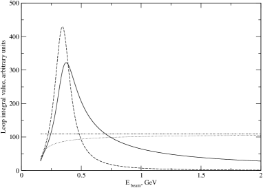
Figure 2: Beam energy dependence of the loop integral (see the text for details) at fixed $Q^{2}=0.05GeV^{2}$ using a Breit-Wigner factor $F_{BW}(W)$ with a) parameters of $\Delta$-resonance (solid line), b) replacing $F_{BW}(W\to\sqrt{s})$ (dashed line), c) same as a) but replacing $F_{BW}(W)$ by 1/5th of its peak value at W=M_R (dotted line), and d) is same as c) but using an analytic formula of Eq.(19) (dash-dotted line).

The master formula for beam SSNA Eq.(28) neglects possible $Q^{2}$ dependence of the invariant form factor of the nucleon Compton amplitude, which was taken in its forward limit during the derivation. In numerical calculations, we estimate additional $Q^{2}$ (= Mandelstam $t$) dependence by introducing an empirical form factor that was measured experimentally in the Compton scattering on the nucleon in the diffractive regime (see Bauer for review). In the following, we use an exponential suppression factor for the nucleon Compton amplitude $\exp{(-BQ^{2}/2)}$, choosing the parameter $B$=8 GeV^-2 that gives a good description of the nucleon Compton cross section from the optical point to $-t\approx$ 0.8 GeV² (see Table V of Ref.Bauer ). The predictions of Eq.(28) combined with the above described exponential suppression are presented in Fig.3 for the electron scattering kinematics relevant for the E158 experiment at SLAC E158 . We choose fit 1 of Ref.block for the total photoproduction cross section in Eq.(28). Exact numerical loop integration of Eq.(2) and the analytic results of Eq.(28) agree with each other with accuracy better than 1%. Contributions from the resonance region ($W^{2}<$ 4 GeV²) were estimated at 10-20% at beam energies of 3 GeV, but rapidly decreasing below 1% at higher energies. We also tested sensitivity of our results to $q_{1,2}^{2}$ dependence of the electroproduction structure function $W_{1}$ (Eq.(23)), taking various empirical parameterizations for it. We found no sensitivity for SLAC E158 kinematics and only moderate sensitivity ($\approx$ 10%) when we extend our calculation to lower energies ($\approx$3 GeV) and higher $Q^{2}\approx$0.5 GeV². For beam energies of 45 GeV, numerical integration shows that more than 95% (80%) of the result for beam SSNA comes from the upper 1/2 (3/4) part of the $W^{2}$-integration range. Based on the results of numerical analysis, we conclude that the formula (28) gives a good description of beam SSNA at small $Q^{2}$ and large $s$ above the resonance region.

We also calculated the contribution of the elastic intermediate proton state to the beam SSNA for high energies and small electron scattering angles using the formalism of Ref.aam and found it to be highly suppressed compared to the inelastic excitations. For the kinematics of SLAC E158 E158 , this suppression is a few orders of magnitude due to different angular and energy behavior of these contributions.

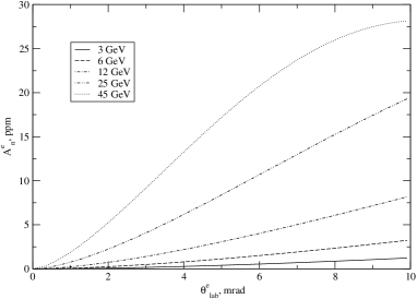
Figure 3: Beam SSNA as a function of the lab scattering angle for different beam energies: 3 GeV (solid line), 6 GeV (dashed line), 12 GeV (dash-dotted line), 25 GeV (dash-double-dotted line) and 45 GeV (dotted line).

Shown in Fig.4 are the calculations for beam SSNA as a function of $Q^{2}$ for different energies of incident electrons. One can see that at small $Q^{2}$, the asymmetry follows $\sqrt{Q^{2}}$ behavior described by Eq.(28), while at higher $Q^{2}$ the asymmetry turns over and starts to decrease due to the introduced exponential form factor $\exp{(-BQ^{2}/2)}$. It can be seen that at fixed $Q^{2}$ the magnitude of beam SSNA is predicted to be approximately constant, as follows from slow logarithmic energy dependence of the total photoproduction cross section.

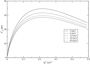
Figure 4: Beam SSNA as a function of $Q^{2}$ for different beam energies. Notation is as in Fig.3.

The latter feature is demonstrated in Fig.5, showing the calculated beam SSNA at fixed $Q^{2}$ in a wide energy range up to $\sqrt{s}$=500 GeV, where we used several parameterizations for the total photoproduction cross section on a proton from Refs.block ; DL , shown in Fig.6. The physical reason for the almost constant photoproduction cross sections at high energies is believed to be soft Pomeron exchange DL , therefore the beam SSNA in the considered kinematics is sensitive to the physics of soft diffraction.

The predicted $Q^{2}$ and energy dependence of beam SSNA, along with its relatively large magnitude, is quite different from the model expectations assuming that no hadronic intermediate states are excited in the TPE amplitude. Our unitarity-based model of small-angle electron scattering predicts the magnitude of the beam SSNA to reach 20-30 ppm in a wide range of beam energies. The good news is that it makes beam SSNA measurable with a presently reached fraction-of-ppm precision of parity-violating electron scattering experiments PViol . On the other hand, the experiments measuring parity-violating observables need to use special care to avoid possible systematic uncertainties due to the parity-conserving beam SSNA. Fortunately, these effects can be experimentally separated using different azimuthal dependence of these asymmetries.

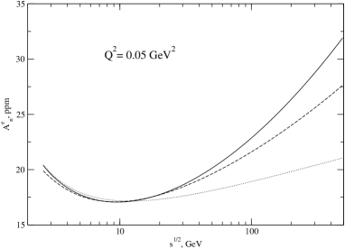
Figure 5: Beam SSNA as a function of c.m.s. energy for fixed Q² = 0.05 GeV² for different parameterizations of the total photoproduction cross section. See Fig.6 for notation.

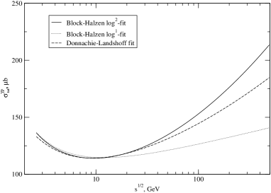
Figure 6: Different parameterizations of total photoproduction cross section at high energies used in the present calculation. A solid (dotted) line is a double-logarithmic fit 1 (single-logarithmic fit 3) from Block and Halzen block and a dashed line is an original Donnachie and Landshoff fit DL .

VI Summary and Conclusions

In the present paper we calculate the beam SSNA for small values of $Q^{2}$ and provide physics arguments for the dominance of contributions from collinear photons in the TPE mechanism. For electron energies above the nucleon resonance region and small $Q^{2}$ the contribution of collinear virtual photons leads to the beam SSNA that is positive and has the order of $m_{e}\sqrt{Q^{2}}\sigma^{\gamma p}_{tot}$, where $\sigma^{\gamma p}_{tot}$ is the total photoproduction cross section on the proton. This quantity is multiplied by the factor of the order unity that includes a combination of double- and single-logarithm terms. The fact that the beam SSNA does not decrease with the beam energy at fixed $Q^{2}$ makes it attractive for experimental studies at higher energies, for example, the energies to be reached at Jefferson Lab after the forthcoming 12-GeV upgrade of CEBAF.

Since the collinear-photon-exchange effect follows from general properties of the rank-3 leptonic tensor, it should also take place at large values of $Q^{2}$ where the collinear kinematics has to contribute with at least logarithmic enhancement. The situation is different for unpolarized (or longitudinally polarized) electrons and for the case of the normal beam polarization. In the first case the leptonic tensor is proportional to the collinear photon 4–momentum $q_{1\beta}$ that leads to cancellation of the collinear region contribution due to the condition of gauge invariance, $q_{1\beta}H_{\mu\alpha\beta}=0$, while this cancellation does not take place for the normal beam polarization. Such behavior of the beam SSNA does not depend on value of $Q^{2}$ and we verified this fact by considering excitations of $N^{*}$ resonances in the intermediate state. It means that the 3-momentum integration in Eq.(2) in general produces logarithmic enhancement in the beam SSNA, unless the dynamics of the non-forward Compton amplitude on a nucleon suppresses this contribution.

The beam SSNA is amplified by the effect similar to the Compton peak in deep-inelastic scattering Spies but with replacement of leptonic and hadronic blocks. Namely, intermediate photon in the TPE box diagram can be collinear to the parent electron and carry 4-momentum that is enough to create a large invariant mass of the intermediate hadronic state. Moreover, the virtuality of this collinear photon is small and such kinematics leads to a dynamical pole (and consequently enhancement) in the box diagram with inelastic hadronic intermediate states. Emission of hard collinear photons is known to enhance helicity-flip effects, as was noted in the original article of T. D. Lee and M. Nauenberg Lee and recently discussed, for example, in the context of radiative muon decay radmuon .

Because of the enhanced collinear-photon exchange contributions, experiments measuring normal SSNA are sensitive to the energy-weighted integrals of the same nucleon Compton amplitudes (namely, their absorptive parts) that can be accessed in Compton scattering experiments where at least one of the photons is real. In contrast, calculations of TPE effects for unpolarized electron scattering require knowledge of the nucleon Compton amplitude with two space-like virtual photons. In relation to normal single-spin asymmetries, we state that the TPE effects in experiments with unpolarized (or longitudinally polarized) electrons, as opposed to the normal polarized electron beams, probe different domains of the non-forward nucleon Compton scattering which can be hidden in the TPE amplitude with inelastic hadronic states. In the first case, the entire 3-dimensional phase space in the TPE loop integration contributes, while the regions of small photon virtualities are suppressed. It justifies the ‘handbag’ approach with Generalized Parton Distributions for these observables, as developed in Ref.Afanas . For the second case, small virtualities of the exchanged photons dominate the TPE integral. In the kinematics $s>>-t$ above the resonance region, the beam SSNA is defined by the total photoproduction cross section that, in turn, is described by (soft) Pomeron exchange. Therefore the soft diffractive (Pomeron) physics dominates the beam SSNA of small-angle elastic electron-proton scattering associated with electron helicity flip, in contrast to the known helicity-conserving property of Pomeron exchange between hadrons.

Large logarithms are also present in the QED radiative corrections to a related observable, beam SSNA of polarized Moller scattering Dixon , where they are caused by initial- and final-state radiation of collinear (real) photons.

When applying the approach Afanas to the beam SSNA, as was done recently in Ref.Mark , the contributions of hard collinear virtual photons are excluded in the ‘handbag’ model of the TPE interaction. Since the collinear photon region contributes with large logarithmic enhancement, the beam SSNA is sensitive to ‘non-handbag’ terms (for example, Regge-exchange terms) in the TPE mechanism, which are important to include in dynamical models of this observable.

Appendix A

Taking into account Eqs. (2) and (27) one can write the beam SSNA at small values of $Q^{2}$ as

$$A_{n}^{e}=\frac{m_{e}\sqrt{Q^{2}}\sigma^{\gamma p}_{tot}}{4\pi^{3}}\frac{F_{1}-\tau F_{2}}{F_{1}^{2}+\tau F_{2}^{2}}\int\frac{d^{3}k}{2E_{k}}\frac{(W^{2}-M^{2})^{2}}{(s-M^{2})^{2}}\frac{Q^{2}}{q_{1}^{2}q_{2}^{2}}\ .$$ (29)

The angular integration in Eq.(29) can be done by introducing the Feynman parameter,

$$\int\frac{d\Omega_{k}}{q_{1}^{2}q_{2}^{2}}=\int\limits_{0}^{1}dy\int\frac{d\Omega_{k}}{[-2m_{e}^{2}+2(kk_{y})]^{2}}\ ,$$

$$k_{y}=yk_{1}+(1-y)k_{2}=(E_{k1};y{\bf{k}_{1}}+(1-y){\bf{k}_{2}}),$$

$$(kk_{y})=E_{k1}E_{k}-2k|{\bf{k}_{y}}|\cos{\theta_{y}},\ \ d\Omega_{k}=d\Phi d\cos{\theta_{y}}\ .$$

Integration over $d\Omega_{k}$ and Feynman parameter $y$ is straightforward, leading to

$$\int\frac{d^{3}k}{2E_{k}}\frac{(W^{2}-M^{2})^{2}}{(s-M^{2})^{2}}\frac{Q^{2}}{q_{1}^{2}q_{2}^{2}}=\frac{\pi}{2}\int_{m_{e}}^{E_{s}}\frac{dE_{k}}{k}(1-z)^{2}L_{1},$$ (30)

where $z=E_{k}/E_{k1}$, and we extended the upper limit up to $E_{k1}$ because the difference between the value of $E_{k}$ at inelastic threshold (when $W^{2}=(m_{\pi}+M)^{2}$) and $E_{k1}$ is negligible at large $s$, and the quantity $L_{1}$ is defined in Eq.(18).

To calculate the integral in Eq.(30), we note first that the region where $k\simeq 0$ does not contribute because of the factor of $L_{1}$. For this reason we can change integration with respect to $E_{k}$ by integration over $k.$ Then we divide the integration region into the following two parts, $0<k<\lambda m_{e}$ and $\lambda m_{e}<k<E_{k1}$, and choose the auxiliary parameter $\lambda$ in such a way that

$$\lambda>>1,\ \lambda m_{e}<<E_{k1}<<\sqrt{Q^{2}}\lambda\ .$$ (31)

In the first region we can neglect $E_{k}$ as compared with $E_{k1}$ and write the corresponding contribution in the form

$$I_{1}=\pi\int\limits_{0}^{\lambda m_{e}}\frac{dk}{k}L_{1}=\int\limits_{0}^{\lambda\sqrt{Q^{2}}/2E_{k1}}\frac{2\pi dz}{\sqrt{1+z^{2}}}\log(z+\sqrt{1+z^{2}})$$

$$=\pi\log^{2}\Big{(}\lambda\frac{\sqrt{Q^{2}}}{E_{k1}}\Big{)}\ .$$ (32)

In the second region the quantity $\eta$ that enters $L_{1}$ is small and we have

$$I_{2}=\pi\int\limits_{z_{\lambda}}^{1}\frac{dz}{z}(1-z)^{2}\Big{(}\log\frac{Q^{2}}{m_{e}^{2}}+2\log\frac{z}{1-z}\Big{)}\ ,$$ (33)

$$z_{\lambda}=\frac{\lambda m_{e}}{E_{k1}}<<1\ .$$

The integration in Eq.(33) gives

$$I_{2}=\frac{\pi}{2}\Big{(}2\log\frac{1}{z_{\lambda}}\log\frac{Q^{2}}{m_{e}^{2}}-2\log^{2}{z_{\lambda}}-3\log\frac{Q^{2}}{m_{e}^{2}}+\frac{2\pi^{2}}{3}+2\Big{)}\ .$$

In the sum $I_{1}+I_{2}$ the auxiliary parameter $\lambda$ is cancelled and we arrive at

$$\int\frac{d^{3}k}{2E_{k}}\frac{(W^{2}-M^{2})^{2}}{(s-M^{2})^{2}}\frac{Q^{2}}{q_{1}^{2}q_{2}^{2}}=$$ (34)

$$\frac{\pi}{4}\Big{(}\log^{2}\frac{Q^{2}}{m_{e}^{2}}-6\log\frac{Q^{2}}{m_{e}^{2}}+\frac{4\pi^{2}}{3}+4\Big{)}\ .$$

References

- (1) P.A.M. Guichon and M. Vanderhaeghen, Phys. Rev. Lett. 91, 142303 (2003); P.G. Blunden, W. Melnitchouk, and J. A Tjon, Phys. Rev. Lett. 91, 142304 (2003); M.P. Rekalo and E. Tomasi–Gustafsson, nucl-th/0307066.
- (2) Y.C. Chen, A.V. Afanasev, S.J. Brodsky, C.E. Carlson, and M. Vanderhaeghen, hep-ph/0403058.
- (3) D. Műller et al., Fortshr. Phys. 42, 2 (1994); A.V. Radyushkin, Phys. Lett. B 385, 333 (1996); A.V. Radyushkin, Phys. Rev. D 56, 5524 (1997); X. Ji, Phys. Rev. Lett. 78, 610 (1997).
- (4) Jefferson Lab proposal PR-04-116, contact person W. Brooks.
- (5) N.F. Mott, Proc. R. Soc.London, Ser. A 135, 429 (1935).
- (6) A.O. Barut and C. Fronsdal, Phys. Rev. 120, 1871 (1960).
- (7) F. Guerin, C. A. Picketty, Nuovo Cim. 32, 971 (1964); J. Arafune, Y. Shimizu, Phys. Rev. D 1, 3094 (1970); U. Gűnther, R. Rodenberg, Nuovo Cim. A 2, 25 (1971); A. De Rujula, J.M. Kaplan and E. De Rafael, Nucl. Phys. B 35, 365 (1971); T.V. Kukhto et al., Preprint JINR–E2–92–556, Feb. 1993.
- (8) A.V. Afanasev, I.V. Akushevich, N.P. Merenkov, hep-ph/0208260.
- (9) S.P. Wells et al., SAMPLE Collaboration, Phys. Rev. C 63, 064001 (2001).
- (10) M. Gorshtein, P.A.M. Guichon, M. Vanderhaeghen, hep-ph/0404206.
- (11) L. Diaconescu and M. J. Ramsey-Musolf, arXiv:nucl-th/0405044.
- (12) F. Maas et al., MAMI /A4 Collaboration, in preparation.
- (13) SLAC E158 Experiment, contact person K. Kumar.
- (14) G. Cates, K. Kumar, D. Lhuiller, spokespersons HAPPEX-2 Experiment, JLab E-99-115: D. Beck, spokesperson JLab/G0 Experiment, JLab E-00-006, E-01-116.
- (15) B. Pasquini and M. Vanderhaeghen, arXiv:hep-ph/0405303.
- (16) R. Tarrach, Nuovo Cim. A 28, 409 (1975).
- (17) B.L.Joffe, V.A. Khose, and L.N. Lipatov, Hard Processes, North Holland, Amsterdam (1984).
- (18) K. Hagiwara et al. [Particle Data Group Collaboration], Phys. Rev. D 66, 010001 (2002).
- (19) T. H. Bauer, R. D. Spital, D. R. Yennie and F. M. Pipkin, Rev. Mod. Phys. 50, 261 (1978) [Erratum-ibid. 51, 407 (1979)].
- (20) M. M. Block and F. Halzen, arXiv:hep-ph/0405174.
- (21) A. Donnachie and P. V. Landshoff, Phys. Lett. B 296, 227 (1992).
- (22) J. Kripfganz, H. J. Mohring and H. Spiesberger, Z. Phys. C 49, 501 (1991).
- (23) T. D. Lee and M. Nauenberg, Phys. Rev. 133 (1964) B1549.
- (24) M. Fischer, S. Groote, J. G. Korner and M. C. Mauser, Phys. Rev. D 67, 113008 (2003), L. M. Sehgal, Phys. Lett. B 569, 25 (2003) [arXiv:hep-ph/0306166]; V. S. Schulz and L. M. Sehgal, arXiv:hep-ph/0404023.
- (25) L. Dixon and M. Schreiber, arXiv:hep-ph/0402221.