Enhanced solar anti-neutrino flux in random magnetic fields

Abstract

We discuss the impact of the recent KamLAND constraint on the solar anti-neutrino flux on the analysis of solar neutrino data in the presence of Majorana neutrino transition magnetic moments and solar magnetic fields. We consider different stationary solar magnetic field models, both regular and random, highlighting the strong enhancement in the anti-neutrino production rates that characterize turbulent solar magnetic field models. Moreover, we show that for such magnetic fields inside the Sun, one can constrain the intrinsic neutrino magnetic moment down to the level of $\mu_{\nu}\lesssim{\rm few}\times 10^{-12}\mu_{B}$ irrespective of details of the underlying turbulence model. This limit is more stringent than all current experimental sensitivities, and similar to the most stringent bounds obtained from stellar cooling. We also comment on the robustness of this limit and show that at most it might be weakened by one order of magnitude, under very unlikely circumstances.

I Introduction

The KamLAND experiment has recently reached an improved sensitivity on a possible electron anti-neutrino component in the solar flux Eguchi:2003gg . Their current limit corresponds to $2.8\times 10^{-2}\%$ of the solar boron $\nu_{e}$ flux, at the $90\%$ C.L., about 30 times better than the previous Super-Kamiokande Gando:2002ub and the recent SNO Aharmim:2004uf limits. Solar anti-neutrinos constitute a characteristic signature of the spin-flavor precession (SFP) mechanism when non-vanishing Majorana neutrino transition magnetic moments Schechter:1981hw interact with solar magnetic fields Schechter:1981hw ; akhmedov:1988uk ; lim:1988tk .

The very first evidence of reactor anti-neutrino disappearance published by the KamLAND collaboration Eguchi:2002dm has already excluded SFP scenarios as solutions to the solar neutrino problem Barranco:2002te . However this evidence still leaves considerable room for sub-leading SFP effects in solar neutrino physics. It is the latest KamLAND limit on the solar electron anti-neutrino flux Eguchi:2003gg , in combination with solar neutrino data, including the recent SNO salt phase results Ahmed:2003kj , that ultimately establishes the robustness of the simplest three-neutrino oscillation description of the solar neutrino data Maltoni:2003da showing how it is essentially stable even in the presence of the SFP mechanism Miranda:2003yh  .

Little is known about the detailed structure of solar magnetic fields and several models have been previously used to analyse the SFP conversion. These solar magnetic field models make different assumptions about the nature (regular or random) of solar magnetic fields, their magnitude, location and typical scales Bykov:1998gv ; Kutvitskii ; Guzzo:1998sb ; akhmedov:2002mf ; Friedland:2002pg . According to the dynamo mechanism the solar magnetic field is generated close to the bottom of the convective zone 1983flma….3…..Z . Following this picture, we assume that the field resides within the solar convective zone Bykov:1998gv ; Kutvitskii ; Guzzo:1998sb . Moreover, in accordance with the present-day understanding of solar magnetic field evolution, the large-scale magnetic field in the solar convective zone is followed by a small-scale random component, whose strength is expected to be comparable to or even larger than that of the regular one.

Insofar as the SFP mechanism is concerned, the main difference between random and regular magnetic field scenarios is that the former generally give rise to an enhanced rate of anti-neutrino production, up to two orders of magnitude when compared to the case of regular fields of the same (average) amplitude. This fact has been used in Ref. Miranda:2003yh in order to obtain more stringent limits on $\mu_{\nu}B$. Moreover, assuming that random magnetic fields are of turbulent origin we were able to extract a limit on the transition magnetic moment itself ($\mu_{\nu}$). We show that, under reasonable assumptions, such bound is comparable to the best astrophysical limit that follows from stellar cooling arguments Raffelt:1990pj . An alternative anaysis of the KamLAND data Eguchi:2003gg using the ”delta-correlated” model for the solar random magnetic field was done in Torrente-Lujan:2003cx .

The main purpose of the present paper is to give a more comprehensive description of the models and analysis already presented briefly in Ref. Miranda:2003yh . First to elucidate the physics of the enhanced anti-neutrino SFP conversion rates in random field models, compared to regular magnetic field scenarios. We show how this follows from the loss of coherence of the spin flavour evolution in a fluctuating environment. Second, we show how in a solar magnetohydrodynamics (MHD) turbulence model of Kolmogorov type one can use the characteristic scaling in this theory in order to obtain a limit on the intrinsic neutrino transition magnetic moment $\mu_{\nu}$.

The paper is organized as follows. In Sec. II we develop a perturbative approach to describe neutrino evolution in the presence of convective–zone random magnetic fields, treating the magnetic interactions as small correction to the oscillation evolution Hamiltonian. This provides a good approximation, fully justified in view of recent KamLAND and solar neutrino data which support the MSW LMA interpretation Maltoni:2003da . We show that neutrinos behave as a “Fourier analyzer” reading off only that spectral harmonic of the two-point magnetic field correlation function whose space period equals the neutrino oscillation length. Our solar magnetic field model is discussed in Sec. III, first within the framework of the simplest piece-constant correlation cell model with one effective correlation scale $L_{0}$, and subsequently within a Kolmogorov–type turbulent magnetic field picture. Our discussion illuminates the difference between SFP anti-neutrino production rates within random and regular fields, as well as the physical meaning of the correlation cell model parameters. The results of our neutrino data analysis of the KamLAND $\bar{\nu}_{e}$ limit and future perspectives are given in Sec. IV. We also present in Sec. V a critique of the robustness of this limit and show that at most it might be weakened by one order of magnitude, under very unlikely circumstances. Finally in Sec. VI we summarize our results.

II Neutrino Evolution

Here we adopt a simplified two-neutrino picture of neutrino evolution, neglecting the angle $\theta_{13}$. As we show in the Appendix this is a good approximation, in view of current neutrino data. Solar neutrino evolution in the presence of a magnetic field involves then only the solar mixing angle where $\theta_{12}\equiv\theta_{sol}\equiv\theta$ and is described by a four–dimensional Hamiltonian Schechter:1981hw ; akhmedov:1988uk ; lim:1988tk ,

$$i\left(\begin{array}[]{l}\dot{\nu}_{eL}\\ \dot{\bar{\nu}}_{eR}\\ \dot{\nu}_{aL}\\ \dot{\bar{\nu}}_{aR}\end{array}\right)=\left(\begin{array}[]{cccc}V_{e}-c_{2}\delta&0&\quad s_{2}\delta&\mu_{\nu}b_{+}(t)\\ 0&-V_{e}-c_{2}\delta&\quad-\mu_{\nu}b_{-}(t)&s_{2}\delta\\ s_{2}\delta&-\mu_{\nu}b_{+}(t)&\quad V_{a}+c_{2}\delta&0\\ \mu_{\nu}b_{-}(t)&s_{2}\delta&\quad 0&-V_{a}+c_{2}\delta\end{array}\right)\left(\begin{array}[]{c}\nu_{eL}\\ \bar{\nu}_{eR}\\ \nu_{aL}\\ \bar{\nu}_{aR}\end{array}\right)~{},$$ (1)

where $\nu_{a}=\nu_{\mu}\cos\theta_{23}-\nu_{\tau}\sin\theta_{23}$ ($\theta_{23}\equiv\theta_{atm}$ is the atmospheric mixing angle); $c_{2}=\cos 2\theta$ and $s_{2}=\sin 2\theta$; $\delta=\Delta m^{2}/4E$ is assumed to be always positive. Note in this approximation the Majorana neutrino transition magnetic moment element $\mu_{\nu}\equiv\mu_{ea}$ describing transitions between neutrino flavour states $\nu_{e}$ and $\nu_{a}$ coincides with the element $\mu_{12}$ characterizing transitions between mass eigenstates $\nu_{1}$ and $\nu_{2}$; $V_{e}(t)=G_{F}\sqrt{2}(N_{e}(t)-N_{n}(t)/2)$ and $V_{a}(t)=G_{F}\sqrt{2}(-N_{n}(t)/2)$ are the neutrino matter potentials for $\nu_{eL}$ and $\nu_{aL}$ in the Sun, given by the number densities of the electrons ($N_{e}(t)$) and neutrons ($N_{n}(t)$). Finally, $b_{\pm}=b_{x}\pm ib_{y}$ denote the magnetic field components which are perpendicular to the neutrino trajectory.

Inside the radiative zone, where the magnetic field is neglected, the evolution of the neutrinos reduces to that implied by the LMA MSW oscillation hypothesis. In order to get an approximate analytic solution for Eq. (1) in the convective zone it is convenient to work in the mass basis. Defining the vectors

$$\nu_{L}=\left(\begin{array}[]{c}\nu_{1L}\\ \nu_{2L}\end{array}\right)\qquad\bar{\nu}_{R}=\left(\begin{array}[]{c}\bar{\nu}_{1R}\\ \bar{\nu}_{2R}\end{array}\right)~{},$$ (2)

we then express the evolution equation in a block form as

$$i\left(\begin{array}[]{l}\dot{{\mathbf{\nu}}}_{L}\\ \dot{\bar{{\mathbf{\nu}}}}_{R}\end{array}\right)=\left(\begin{array}[]{cc}H_{osc}&H_{mag}\\ H_{mag}^{\dagger}&\bar{H}_{osc}\end{array}\right)\left(\begin{array}[]{c}\nu_{L}\\ \bar{{\nu}}_{R}\\ \end{array}\right)~{},$$ (3)

where

$$H_{osc}=\left(\begin{array}[]{cc}E_{1L}&-i\dot{\theta}_{m}\\ i\dot{\theta}_{m}&E_{2L}\\ \end{array}\right),\qquad\bar{H}_{osc}=\left(\begin{array}[]{cc}E_{1R}&-i\dot{\bar{\theta}}_{m}\\ i\dot{\bar{\theta}}_{m}&E_{2R}\end{array}\right)$$ (4)

and,

$$H_{mag}=\left(\begin{array}[]{ccc}-\mu_{\nu}b_{+}e^{i\Psi}\sin(\bar{\theta}_{m}-\theta_{m})&&\mu_{\nu}b_{+}e^{i\Psi}\cos(\bar{\theta}_{m}-\theta_{m})\\ -\mu_{\nu}b_{+}e^{i\Psi}\cos(\bar{\theta}_{m}-\theta_{m})&&-\mu_{\nu}b_{+}e^{i\Psi}\sin(\bar{\theta}_{m}-\theta_{m})\end{array}\right)$$ (5)

with $\Psi=1/2\int{[V_{e}(t)+V_{a}(t)]dt}$. The neutrino eigen-energies $E_{iL}$ are defined by

$$E_{iL}=\mp\sqrt{(V-\delta c_{2})^{2}+(\delta s_{2})^{2}}\,,$$ (6)

where $V=(V_{e}-V_{a})/2$ and the minus (plus) sign corresponds to the energy state with $i=1$ ($2$). The solar neutrino mixing angle in matter is given as

$$\tan 2\theta_{m}=-\frac{\delta s_{2}}{V-\delta c_{2}}\,.$$ (7)

Similar expressions for the anti-neutrino eigen-energies and matter mixing angle, $E_{iR}$ and $\bar{\theta}_{m}$, are easily obtained by changing the sign of the matter potential, $V\to-V$, in Eqs. (6) and (7).

In the region of neutrino oscillation parameters indicated by current neutrino data Maltoni:2003da , $\delta=\delta_{\rm LMA}$ and $\theta=\theta_{\rm LMA}$, the matter effect in the convective zone turns out to be rather small, since the ratio of the matter potential $V$ to $\delta_{{\rm LMA}}$ is at most around $\sim 10^{-2}$, at the bottom of the convective zone. This allows us to expand the neutrino eigen-energies in powers of $V/\delta$

$$E_{iL}\simeq\mp\delta\left[1-\frac{V}{\delta}c_{2}+\frac{V^{2}}{\delta^{2}}s_{2}^{2}+O\left(\frac{V^{3}}{\delta^{2}}\right)\right]$$ (8)

and similarly the neutrino mixing angle in matter may be expressed as

$$\theta_{m}\simeq\theta+\frac{V}{\delta}s_{2}-\frac{V^{2}}{\delta^{2}}(1+s_{2}^{2})\tan 2\theta+O\left(\frac{V^{3}}{\delta^{2}}\right)~{}.$$ (9)

An analogous estimate gives an upper bound on the mixing angle derivative, $|\dot{\theta}_{m}|/\delta\lesssim 2\times 10^{-5}$ and

$$\left|\frac{\dot{\theta}_{m}}{\mu_{\nu}b_{\perp}}\right|\lesssim 5\times 10^{-3}\left(\frac{10^{-11}\mu_{B}}{\mu_{\nu}}\right)\left(\frac{100{\rm kG}}{b_{\perp}}\right)\,.$$ (10)

with similar approximations valid for anti-neutrinos.

Therefore we can safely neglect all powers of $V/\delta$, along with $\dot{\theta}_{m}$ and $\dot{\bar{\theta}}_{m}$. In this approximation the $(4\times 4)$ evolution equation decouples into two $(2\times 2)$ equations

$$i\left(\begin{array}[]{l}\dot{\nu}_{1L}\\ \dot{\bar{\nu}}_{2R}\end{array}\right)=\left(\begin{array}[]{cc}-\delta&\mu b_{+}(t)e^{i\Psi}\\ \mu b_{-}(t)e^{-i\Psi}&\delta\end{array}\right)\left(\begin{array}[]{c}\nu_{1L}\\ \bar{\nu}_{2R}\end{array}\right)~{},$$ (11)

$$i\left(\begin{array}[]{l}\dot{\nu}_{2L}\\ \dot{\bar{\nu}}_{1R}\end{array}\right)=\left(\begin{array}[]{cccc}\delta&-\mu b_{+}(t)e^{i\Psi}\\ -\mu b_{-}(t)e^{-i\Psi}&-\delta\\ \end{array}\right)\left(\begin{array}[]{c}\nu_{2L}\\ \bar{\nu}_{1R}\end{array}\right)~{},$$ (12)

describing spin-flavour precession of the two mass-eigenstate pairs. In the absence of magnetic fields the neutrino eigenstates propagate independently across the convective zone. When the magnetic field is switched on one obtains a mixing, characteristic of the spin flavour precession mechanism Schechter:1981hw . This turns out to be rather small, a fact that greatly simplifies the problem of solving the evolution equation. For this we consider the parameter $\kappa$ defined as

$$\kappa=\frac{\mu_{\nu}^{2}b_{\perp}^{2}}{\delta^{2}}=2.5\times 10^{-5}\left(\frac{\mu_{\nu}}{10^{-11}\mu_{B}}\right)^{2}\left(\frac{b_{\perp max}}{100{\rm kG}}\right)^{2}\left(\frac{7\times 10^{-5}{\rm eV^{2}}}{\Delta m^{2}}\right)^{2}\left(\frac{E}{10{\rm MeV}}\right)^{2}~{}.$$ (13)

The smallness of $\kappa$ allows us to expand the neutrino survival probabilities at the surface of the Sun in powers of $\kappa$, to any given desired accuracy in perturbation theory. The matter effect akhmedov:1988uk ; lim:1988tk is also rather small, and is fully encoded by the phase $\Psi$, so that when $\Psi\to 0$ one recovers the vacuum result of Ref. Schechter:1981hw .

From Eqs. (11) and (12) we find that to leading order in $\kappa$ the neutrino mass eigenstate probabilities at the surface of the Sun can be written in the form

$$|\nu_{1L}|^{2}_{R_{\odot}}=P_{1}(1-\eta),\qquad|\nu_{2R}|^{2}_{R_{\odot}}=P_{1}\eta~{},$$ (14)

$$|\nu_{2L}|^{2}_{R_{\odot}}=P_{2}(1-\eta),\qquad|\nu_{1R}|^{2}_{R_{\odot}}=P_{2}\eta~{},$$ (15)

(note that unitarity is fulfilled), where the key small parameter $\eta$ is given by

$$\eta=\frac{\mu^{2}}{2}\int^{L}_{0}dt_{1}\int^{L}_{0}dt_{2}[b_{+}(t_{1})b_{-}(t_{2})e^{-2i\delta(t_{1}-t_{2})}+c.c.]~{}.$$ (16)

Here $L$ is the width of the convective zone and $P_{i}=|\nu_{iL}(r=0.7R_{\odot})|^{2}$ denote the probabilities that solar neutrinos reach the bottom of the convective zone in a given mass state, calculated numerically in the LMA-MSW oscillation picture, similar to the method used in Maltoni:2003da .

The probabilities for neutrinos to be detected in flavour states $\alpha=e,\mu,\bar{e},\bar{\mu}$, $P_{e\alpha}$, are then given by

$$P_{ee} = \left[P_{1}P_{1e}+P_{2}P_{2e}+2\sqrt{P_{1}P_{2}P_{1e}P_{2e}}\cos\xi_{1}\right](1-\eta),$$ (17)

$$P_{e\mu} = \left[P_{1}P_{1\mu}+P_{2}P_{2\mu}-2\sqrt{P_{1}P_{2}P_{1\mu}P_{2\mu}}\cos\xi_{1}\right](1-\eta),$$ (18)

$$P_{e\bar{e}} = \left[P_{2}P_{\bar{1}\bar{e}}+P_{1}P_{\bar{2}\bar{e}}-2\sqrt{P_{2}P_{1}P_{\bar{1}\bar{e}}P_{\bar{2}\bar{e}}}\cos\xi_{2}\right]\eta,$$ (19)

$$P_{e\bar{\mu}} = \left[P_{2}P_{\bar{1}\bar{\mu}}+P_{1}P_{\bar{2}\bar{\mu}}+2\sqrt{P_{2}P_{1}P_{\bar{1}\bar{\mu}}P_{\bar{2}\bar{\mu}}}\cos\xi_{2}\right]\eta.$$ (20)

Here $P_{i\alpha}$ is the $\nu_{i}\to\nu_{\alpha}$ conversion probability from the surface of the Earth to the detector. The phases $\xi_{k}$ ($k=1,2$) characterize the evolution in vacuum from the Sun to the Earth, and are given by

$$\xi_{k}=\frac{\Delta m^{2}(D+L-R_{\odot})}{2E}+\phi_{k}\,,$$ (21)

where $D$ is the Sun-Earth distance, $\phi_{k}$ contain the phases due to propagation in the Sun up to the bottom of the convective zone and in the Earth. We have checked that $\phi_{k}$ can be safely neglected for our purposes.

In summary, neutrino evolution can be understood as follows:

• neutrinos, generated in the solar core, undergo LMA MSW conversion and enter the convective zone as a coherent mixture of $\nu_{eL}$ and $\nu_{aL}$. By numerically solving the corresponding $(2\times 2)$ MSW evolution problem we obtain the amplitudes $\nu_{eL}(0)$ and $\nu_{aL}(0)$ at the bottom of the convective zone, which are then used as initial values for neutrino propagation across the convective zone.

• neutrino evolution within the convective zone is considered as approximately vacuum oscillations modulated by a small spin-flavour conversion Schechter:1981hw . This is treated in leading order in the small expansion parameter $\kappa$, Eq. (13).

• the neutrino survival and conversion probabilities, defined at the solar surface, are then evolved to the detector taking into account regeneration in the Earth.

This way neutrino and anti-neutrino yields are determined and used in the analysis of solar neutrino and KamLAND data.

III Magnetic Field Model

The main goal of this section is to calculate the parameter $\eta$ in Eq. (16) characterizing the solar anti-neutrino production rate to first order in the small expansion parameter $\kappa$ in Eq. (13) describing neutrino propagation in the framework of different solar magnetic field models.

Different approaches have been used in order to describe neutrino propagation in the fluctuating matter density or random magnetic field environments. Since the origin of the media fluctuations is unknown, we stick to the simplest “white” noise description, which involves just two parameters: the typical correlation scale and its characteristic amplitude.

The “delta-correlated” model described by

$$\left\langle b_{\perp}(r_{1})b_{\perp}(r_{2})\right\rangle=\bar{b_{\perp}^{2}}\left(\frac{r_{1}+r_{2}}{2}\right)L_{0}\delta(r_{1}-r_{2})$$

has been used both for the case of matter density fluctuations Loreti:1994ry ; Nunokawa:1996qu ; Balantekin:2003qm ; Guzzo:2003xk , as well as random magnetic fields Nicolaidis:1991da ; Bykov:1998gv ; Semikoz:1998ef ; Torrente-Lujan:2003cx . This choice of correlator has the virtue that it allows for analytical solutions to the neutrino evolution equations. It suffers from an important limitation, namely that the allowed spatial scales, $L_{0}$, of fluctuations should be less than typical neutrino oscillation lengths $\lambda_{osc}=4\pi E/\Delta m^{2}$. However, it so happens that the strongest conversion effect takes place when these two parameters are comparable Burgess:1997mz .

Because of this one needs to go at least one step further and consider the so called “piece-constant” model. For the case of matter density fluctuations this has been used in Refs. Burgess:1997mz ; Burgess:2002we ; Burgess:2003su and for random magnetic fields it was applied in Bykov:1998gv .

In what follows (Sec. III.1) we adopt this piece-constant model, whose correlator is described by,

$$\left\langle b_{\perp}(r_{1})b_{\perp}(r_{2})\right\rangle=\bar{b_{\perp}^{2}}\left(\frac{r_{1}+r_{2}}{2}\right)\phantom{0}, {\rm if} |r_{1}-r_{2}|\leq L_{0}$$

$$\left\langle b_{\perp}(r_{1})b_{\perp}(r_{2})\right\rangle=0\phantom{\bar{b_{\perp}^{2}}\left(\frac{r_{1}+r_{2}}{2}\right)}, {\rm if} |r_{1}-r_{2}|>L_{0}.$$

In other words, the fluctuation correlation function is modeled as a step-function. We refer to this as “simplest random magnetic field model”.

Note that in these models the typical correlation scale is in general a free unknown parameter. One may go a step further if one has more information about the nature of the assumed fluctuations. For instance, a detailed analysis of how density fluctuations, in the form of helioseismic waves, can affect the MSW neutrino oscillations was introduced in Ref. Bamert:1998jj . In the discussion we give in Sec. III.2 we use the solar MHD turbulence model in order to describe the nature of the solar random magnetic fields. These are described by a magnetic field correlation tensor

$$\left\langle b_{i}(r_{1})b_{j}(r_{2})\right\rangle=M_{ij}(r_{1},r_{2})\,,$$

whose specific form will be given below (Eq. (27)). As a result the separate dependence on the correlation scale and the amplitude of fluctuations is replaced by a dependence on a specific combination of these parameters, $\varepsilon$ in Eq. (35). This has the advantage of expressing the final neutrino fluxes in terms of a single effective parameter which varies over a relatively narrow range.

III.1 Simplest random field model

As already mentioned, current views on solar magnetic field evolution suggest that the mean large-scale magnetic field is followed by a comparable small-scale random magnetic field component. Such random small-scale magnetic field is not directly traced by sunspots or other tracers of solar activity. Dynamically, this field propagates through the convective zone and photosphere drastically decreasing in strength. While we lack a direct reliable observational estimate of its amplitude, one finds that the ratio of the random to regular magnetic field amplitudes may be as large as 50-100, as it is not clear at what stage the dynamo mechanism saturates. This issue has been very actively discussed in the literature (see, e.g., 1983flma….3…..Z ; Subramanian:1999mr and references therein).

The simplest random convective–zone solar magnetic field model is obtained by imagining that the convective zone consists of a set of correlation cells of volume $L_{0}^{3}$ where the random magnetic field is assumed uniform, fields in adjacent cells being uncorrelated. In this picture we treat the small-scale random magnetic fields in terms of a single effective scale $L_{0}$ characterizing the size of the correlation cells. We also assume that within each cell different magnetic field components transversal to the neutrino trajectory are independent random variables with zero mean value (for a more detailed discussion see, for example, Ref. Bykov:1998gv ). That is, a given realization of the random magnetic field along the neutrino path is a stationary random process described by Gaussian statistics. It is also assumed that in order to satisfy divergence-less condition, $\nabla\cdot\mathbf{B}=0$, the magnetic field strength changes smoothly at the boundaries between adjacent cells. This simplified model seems reasonable since we do not expect a strong influence of details of the random magnetic field structure near the layers separating adjacent domain cells.

In order to estimate $\eta$ in Eq. (16) we divide the range of integration into a set of equal intervals of correlation length $L_{0}$ and average over random magnetic fields in each correlation cell,

$$\left\langle\eta\right\rangle=\frac{1}{2}\mu^{2}\sum^{N}_{k=1}\sum^{N}_{l=1}\int^{kL_{0}}_{(k-1)L_{0}}dt_{1}\int^{lL_{0}}_{(l-1)L_{0}}dt_{2}\left\langle b_{+}(t_{1})b_{-}(t_{2})e^{-2i\delta(t_{1}-t_{2})}+c.c.\right\rangle\,,$$ (22)

this results in the final equation

$$\left\langle\eta\right\rangle=\left(\sum^{N}_{n=1}\mu^{2}\bar{b^{2}}_{\perp n}\right)\frac{\sin^{2}\left(\delta\cdot L_{0}\right)}{\delta^{2}}\,,$$ (23)

where $\bar{b^{2}}_{\perp n}$ is the averaged square of the random magnetic field in the $n$-th correlation cell. We assume that the root mean square (rms) field varies smoothly along the neutrino trajectory. One therefore clearly sees the cumulative effect characterizing neutrino propagation in random magnetic fields, implied by the sum in Eq. (23). For the simple case where all rms field amplitudes in different cells are equal to some common magnetic field value the above result gets proportional to the number of correlation cells traversed by the neutrino, $N=L/L_{0}$.

In contrast, for regular magnetic fields the situation is different. The neutrino to anti-neutrino conversion probability after traversing the convective zone with a constant regular magnetic field of the same amplitude is proportional to

$$\eta=\frac{\mu_{\nu}^{2}b_{\perp}^{2}}{\delta^{2}+\mu_{\nu}^{2}b_{\perp}^{2}}\sin^{2}\left(\sqrt{\delta^{2}+\mu_{\nu}^{2}b_{\perp}^{2}}L\right)=\frac{\mu_{\nu}^{2}b_{\perp}^{2}}{\delta^{2}}\sin^{2}(\delta\cdot L)+O\left((\frac{\mu_{\nu}^{2}b_{\perp}^{2}}{\delta^{2}})^{2}\right)\approx\frac{\mu_{\nu}^{2}b_{\perp}^{2}}{2\delta^{2}}~{},$$ (24)

that is, what would be expected after passing only one cell.

Therefore in the random magnetic field case one obtains a sizable enhancement of the neutrino conversion probability as compared with the case of a constant magnetic field of the same amplitude. This enhancement is explained by the fact that the random nature of the magnetic field destroys the coherence in the neutrino evolution. Therefore, instead of adding amplitudes one have to add probabilities rez04 .

Finally, in order to take account of the shape of the rms random field profile we introduce a factor

$$S^{2}=\frac{1}{N}\sum\limits_{n=1}^{N}\frac{\bar{b_{n}^{2}}}{b_{\perp max}^{2}},$$ (25)

which is $S=1$ for constant rms field and of the order of unity for other sufficiently wide spatial profiles, e.g. $S\approx 0.579$ for “smooth” profile Bykov:1998gv , $S\approx 0.577$ for triangle profile Guzzo:1998sb , $S\approx 0.782$ for Kutvitsky-Solov’ev profile Miranda:2000bi . An alternative estimate of typical shape factors comes from the assumption that the magnetic energy density globally follows the approximate solar density profile with the scale height $H=0.1R_{\odot}$, leading to $S\approx\sqrt{H/L}\approx 1/\sqrt{3}\approx 0.57$.

Using the above definition of the shape factor one can rewrite Eq. (23) as

$$\left\langle\eta\right\rangle=\frac{\mu^{2}b^{2}_{\perp max}}{\delta^{2}}S^{2}~{}\frac{L}{L_{0}}~{}\sin^{2}(\delta\cdot L_{0})\,,$$ (26)

where $b^{2}_{\perp max}$ is the maximal value of the transverse magnetic field. This shows that different random magnetic field models can be effectively characterized by two parameters, $b^{2}_{\perp max}S^{2}$ and $L_{0}$.

III.2 Magnetohydrodynamic turbulence models

A well motivated class of magnetic field models can be considered for which the number of parameters can be further reduced by eliminating reference to the effective scale $L_{0}$. The relevant average $\left\langle(b_{+}(t_{1})b_{-}(t_{2})\right\rangle$ of the transverse components of the magnetic fields can be characterized by introducing the two-point magnetic field correlation tensor as $M_{ij}=\left\langle b_{i}(\mathbf{r}_{1})b_{j}(\mathbf{r}_{2})\right\rangle$.

For the case of isotropic, homogeneous and non-helical random magnetic fields $M_{ij}$ is separated as

$$M_{ij}~{}=~{}M_{N}\left(\delta_{ij}-\frac{r_{i}r_{j}}{r^{2}}\right)+M_{L}~{}\frac{r_{i}r_{j}}{r^{2}}~{}.$$ (27)

where $\mathbf{r}=\mathbf{r}_{1}-\mathbf{r}_{2}$. The longitudinal ($M_{L}$) and transverse ($M_{N}$) correlation functions depend only on the separation distance between the two points, $r=|\mathbf{r}_{1}-\mathbf{r}_{2}|$. Given that $\mathbf{\nabla}\cdot\mathbf{B}=0$, one can write

$$M_{N}(r)=\frac{1}{2r}\frac{\partial}{\partial r}(r^{2}M_{L}(r))~{}.$$ (28)

One can generalize the above definition of the correlation function in Eq. (27) so as to cover the case of media which are isotropic and homogeneous only locally. This can be done by expressing the correlator in factorized form as MoninYaglom

$$M_{N}(\mathbf{r_{1}},\mathbf{r_{2}})=F\left(\frac{\mathbf{r_{1}}+\mathbf{r_{2}}}{2}\right)K_{N}(|\mathbf{r_{1}}-\mathbf{r_{2}}|)~{},$$ (29)

where the random magnetic field profile factor $F$ depends on the center-of-mass position of the two points $\mathbf{r_{1}}$ and $\mathbf{r_{2}}$ and the local correlator $K_{N}(r)$ coincides with the one characterizing the isotropic and homogeneous case, $M_{N}(r)$, given in Eq. (27).

The above form provides a reasonable description for solar magnetic field profiles. Indeed, typical solar rms field profiles ($F$) vary on scales of the order of the density scale height $H\approx 70000~{}\rm{km}$. On the other hand $K_{N}$ involves averaging on much smaller scales $\delta^{-1}$ related to the neutrino oscillation length, about hundred kilometers for the LMA-MSW case.

Substituting Eq. (27) into Eq. (16) and restricting the coordinates to the neutrino path, we get

$$\left\langle\eta\right\rangle=\mu^{2}\int^{L}_{0}dz_{1}\int^{L}_{0}dz_{2}M_{N}(z_{1},z_{2})\cos[2\delta(z_{1}-z_{2})]~{},$$ (30)

where $z_{1}$ and $z_{2}$ are two points on the neutrino trajectory.

Substituting Eq. (29) into Eq. (30), changing variables and rearranging we get

$$\left\langle\eta\right\rangle=4\mu^{2}S^{2}L\int^{\infty}_{0}d\xi K_{N}(\xi)\cos(2\delta\cdot\xi)~{},$$ (31)

where the integration is extended to infinity because of $\delta\cdot H\gg 1$ and the shape factor $S^{2}$ is defined as a continuous analogue of Eq. (25)

$$S^{2}=\frac{1}{L}\int\limits_{0}^{L}\frac{\bar{b_{\perp}^{2}}(z)}{b_{\perp max}^{2}}dz\,.$$ (32)

In order to estimate $K_{N}(\xi)$ we assume that magnetic field evolution in the solar convective zone is due to the highly developed steady-state MHD turbulence treated within the Kolmogorov scaling theory Kolmogorov:1941 ; Kolmogorov:1991 ; 1983flma….3…..Z . In other words, for large magnetic Reynolds number, $R_{m}\sim 10^{8}$ 1983flma….3…..Z , the solar MHD turbulence is pumped by the largest eddy motion that follows from the interplay between convection and differential rotation of the Sun. The size of the largest eddies, $L_{{\rm max}}$, may be associated with the solar granule size of the order of $1000~{}{\rm km}$. Dynamo enhancement subsequently results in the direct cascade of the energy of MHD fluctuations to smaller scales . The smallest scale at which turbulent motion starts to decay transferring energy into heat is the dissipative scale defined through $l_{{\rm diss}}=L_{{\rm max}}R_{m}^{-3/4}\approx 1~{}{\rm m}$ .

Within the inertial range, $l_{{\rm diss}}<l<L_{{\rm max}}$, the similarity arguments of the Kolmogorov theory require the turbulent hydrodynamic (HD) kinetic energy spectrum to scale as $E_{{\rm HD}}\sim k^{-5/3}$, where $k\sim 1/l$ is the wave number of the eddies of size $l$ Kolmogorov:1941 ; Kolmogorov:1991 ; 1983flma….3…..Z . Similar qualitative arguments applied to the MHD case imply that the corresponding Iroshnikov-Kraichnan scaling law can be taken as $E_{{\rm MHD}}\sim k^{-3/2}$ 1983flma….3…..Z . However recent theoretical results and numerical simulations suggest that the simpler HD Kolmogorov spectrum can actually be used even for the MHD case Goldreich ; Cho . For our purposes the difference in the power-law exponents turns out to be not specially important so that, we take for definiteness the Kolmogorov value $p=5/3$. Generalization to arbitrary $p$’s is straightforward. See details below.

Let us model the longitudinal correlation function $K_{L}(r)$ as in hydrodynamics MoninYaglom

$$K_{L}(l)=\frac{\bar{b^{2}}}{3}\frac{2^{2/3}}{\Gamma(1/3)}\left(\frac{l}{L_{\rm max}}\right)^{1/3}K_{1/3}\left(\frac{l}{L_{\rm max}}\right)~{},$$ (33)

where $\Gamma(x)$ is the gamma-function, $K_{\mu}(x)$ is the McDonald function of index $\mu$ and $\bar{b^{2}}$ is the squared rms magnetic field on scale $L_{\rm max}$. The model function correctly reproduces required asymptotics of the Kolmogorov theory:

• $K_{L}(0)=\left\langle b_{z}^{2}(z)\right\rangle=\bar{b^{2}}/3$ ,

• $K_{L}(0)-K_{L}(l)\sim{l}^{2/3}$ for $l\ll L_{\rm max}$ .

Using Eq. (28) and Eq. (33) and taking into account that $2\delta\cdot L_{{\rm max}}\gg 1$ we finally perform the integration in Eq. (31) and obtain

$$\left\langle\eta\right\rangle\simeq\frac{\sqrt{\pi}}{3}\frac{2^{1/3}\Gamma(5/6)}{\Gamma(1/3)}\frac{{\mu}^{2}\bar{b^{2}}S^{2}LL_{{\rm max}}}{(\delta\cdot L_{{\rm max}})^{5/3}}\simeq 0.3\frac{{\mu}^{2}\bar{b^{2}}S^{2}}{{\delta}^{2}}\frac{\delta\cdot L}{(\delta\cdot L_{\rm{max}})^{2/3}}~{}.$$ (34)

which leads, in normalized units, to

$$\ \left\langle\eta\right\rangle\simeq 3\times 10^{-3}\mu_{11}^{2}\varepsilon^{2}S^{2}\left(\frac{7\times 10^{-5}{\rm eV}^{2}}{\Delta m^{2}}\right)^{5/3}\left(\frac{E}{10{\rm MeV}}\right)^{5/3}\,,$$ (35)

where $\mu_{11}$ is the magnetic moment in units of $10^{-11}\mu_{B}$, and the ratio $\varepsilon=(b/100~{}{\rm kG})/(L_{{\rm max}}/1000~{}{\rm km})^{1/3}$.

The ratio $\varepsilon$ is not known precisely, but one may estimate it assuming equipartition between kinetic energy of hydrodynamic fluctuations and the rms magnetic energy at the largest (most energetic) scale $L_{max}$ 1983flma….3…..Z

$$\frac{\rho\bar{v^{2}}}{2}\approx\frac{\bar{b}^{2}}{8\pi}$$ (36)

Taking $v\sim 3\times 10^{4}{\rm cm}/{\rm s}$ and $\rho\sim 1~{}{\rm g/cm}^{3}$  1991sun..book…..S we obtain typical amplitude for magnetic field fluctuations $b\sim 100$ kG at the scale $L_{max}=1000$ km. Assuming that $b\approx 50-100$ kG and that the shape factor $S$ lies in the range between 0.5 and 1 we estimate that the product $\varepsilon S$ may vary in the interval $0.25<\varepsilon S<1$.

Before concluding this section we note that both types of magnetic field models lead to qualitatively similar results for the neutrino conversion parameter $\left\langle\eta\right\rangle$ when the magnetic field correlation scale is chosen to coincide with neutrino oscillation length $\lambda_{osc}$. Indeed, in accordance with the Kolmogorov scaling law $\bar{b^{2}}/(\delta\cdot L_{\rm{max}})^{2/3}\simeq\lambda_{\rm osc}^{2/3}\cdot\bar{b^{2}}/L_{\rm{max}}^{2/3}=\bar{b}_{\lambda_{\rm osc}}^{2}$ is the squared rms field at the scale $\lambda_{\rm osc}$. This implies that Eq. (26) goes into Eq. (34) when making the replacement $\delta\cdot L\sim L/\lambda_{\rm osc}$. This happens because in the context of the turbulent magnetic field model neutrinos effectively feel only one scale, namely their oscillation length.

IV Limits on neutrino magnetic moments

In this section we analyze the limit on electron anti-neutrino flux published by KamLAND Eguchi:2003gg . In Ref. Miranda:2003yh we showed how this limit makes the determination of neutrino oscillation parameters, $\Delta m^{2}_{sol}$ and $\theta_{sol}$, extremely robust against possible existence of spin-flavor conversions. This can be used in order to determine the allowed regions of solar neutrino oscillation parameters independently of the magnetic field and magnetic moment parameters.

Using the standard $\chi^{2}$ procedure (see Barranco:2002te and references therein) and taking into account full set of solar as well as KamLAND reactor neutrino data we have re-determined the allowed regions of solar neutrino oscillation parameters, $\Delta m^{2}_{sol}$ and $\theta_{sol}$, within the recent version of Standard Solar Model (BP04) Bahcall:2004fg . The results are presented as shaded regions in Fig. 1.

Figure 1: Allowed regions for $\Delta m^{2}_{sol}$ and $\theta_{sol}$ from solar and KamLAND neutrino experiments at 90%, 95%, 99% and 99.73% C.L. The curves are electron anti-neutrino iso-flux contours for $L_{0}=100$ km, plotted for different $\mu_{11}Sb_{\perp}$ values indicated in kG, and fixing the anti-neutrino production at the current KamLAND limit. For values above 55 kG or so the high LMA region is ruled out.

Let us first consider the simple random magnetic field model described in Sec. III.1. In this case neutrino conversion probabilities depend both on the oscillation parameters, $\Delta m^{2}_{sol}$ and $\theta_{sol}$, as well as the parameters $\mu^{2}_{\nu}b^{2}_{\perp_{max}}S^{2}$ and $L_{0}$ describing the random magnetic field model. Using Eqs. (19) and (23) we have calculated the predicted electron anti-neutrino flux. In Fig. 1 we show, for a fix value of $L_{0}=100$ km and $S^{2}=1$, the curves that correspond to an electron anti-neutrino yield of $2.8\times 10^{-4}\phi_{B}$. It is clear that a better determination of the solar mixing angle by future experiments will not substantially improve the limits on the parameters $\mu^{2}_{\nu}b^{2}_{\perp_{max}}S^{2}$ and $L_{0}$ which are mainly restricted by the solar anti-neutrino flux limit. In contrast note that an improved determination of the solar mass splitting at KamLAND will play an important role in pinning down the magnetic field parameters.

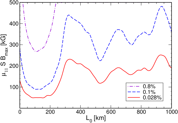
Figure 2: Upper bound on $\mu_{11}Sb_{\perp}$ for a random field with spatial scale $L_{0}$ allowed by the 90% C. L. region of $\Delta m^{2}_{sol}$ and $\theta_{sol}$. The solid line shows the allowed values coming from the current KamLAND limit on $\phi_{\bar{\nu}_{e}}$. For comparison we also give the limits that would correspond to $\phi_{\bar{\nu}_{e}}=0.1\%$ and $\phi_{\bar{\nu}_{e}}=0.8$ % of $\phi_{B}$.

In order to determine the restrictions on these parameters we have imposed that the anti-neutrino yield should not exceed the current experimental bound, $2.8\times 10^{-4}\phi_{B}$ within the presently allowed 90% C.L. region of the ($\Delta m^{2}_{sol}$, $\theta_{sol}$) plane. The results of this analysis are shown in Fig 2. The limits on $\mu^{2}_{\nu}b^{2}_{\perp_{max}}S^{2}$ versus $L_{0}$ correspond to different values of electron anti-neutrino fluxes. The lower curve represents the current upper bound on the product of magnetic moment and magnetic field which follows from the recent KamLAND bound in Ref. Eguchi:2003gg . This is compared with the original sensitivity expected by the KamLAND collaboration Busenitz:1998 (dashed line) and with the Super-K Gando:2002ub bound (dot-dashed line). One can see how Fig. 2 quantitatively confirms the expectation that the strongest limit on $\mu^{2}_{\nu}b^{2}_{\perp}S^{2}$ corresponds to the case when the correlation scale $L_{0}$ is of the same order as the neutrino oscillation length, $\lambda_{osc}\approx 100-200$km.

As discussed in section III.2, solar MHD turbulence provides an attractive framework for the solar magnetic field model, in which the anti-neutrino production probability depends only on one extra parameter: $\mu^{2}_{\nu}\varepsilon^{2}S^{2}$. As we did above, we first determine the values of $\mu^{2}_{\nu}\varepsilon^{2}S^{2}$ that produce an electron anti-neutrino yield of $0.028$ % $\phi_{B}$. In Fig. 3 we have shown curves corresponding to different values of $\mu_{11}\varepsilon S$. Similarly to the case of the simplest random field model one sees that an improved determination of solar neutrino mixing angle will not limit $\mu_{\nu}\varepsilon S$ significantly better than the current constraint. In contrast a better determination of the solar mass splitting at KamLAND will be useful.

Following the same approach as before we have determined the limit on $\mu_{\nu}\varepsilon S$ taking into account the currently 90% C.L. allowed region of solar neutrino oscillation parameters. As we have already seen in Sec. III.2, a reasonable estimate of the allowed range for $\varepsilon S$ is $0.25<\varepsilon S<1$. Therefore, in contrast to the previous models, with random or regular fields, we can now, to within a factor of four, extract direct restriction on the intrinsic neutrino magnetic transition moment $\mu_{\nu}$. This is indicated in Fig. 4. The lowest horizontal line represents current limit on the solar electron anti-neutrino flux from the KamLAND Eguchi:2003gg experiment. On the other hand our bounds on $\mu_{\nu}$ are given by the crossings of the lines delimiting the dark band with the horizontal line labeled KamLAND. From the Fig. 4 one sees that $\mu_{\nu}\leq 5\times 10^{-12}\mu_{B}$ Miranda:2003yh . For comparison the best current laboratory limit by the MUNU experiment ($\mu_{\nu}<1.0\times 10^{-10}\mu_{B}$ at 90% C.L.) Daraktchieva:2003dr is also indicated. This should be compared with the best astrophysical limit, estimated as $\mu_{\nu}<3.0\times 10^{-12}\mu_{B}$ Raffelt:1990pj . As discussed in Sec. V under unlikely circumstances this bound might be weakened by at most one order of magnitude. This would correspond to the tilted line delimiting the hatched band from the right.

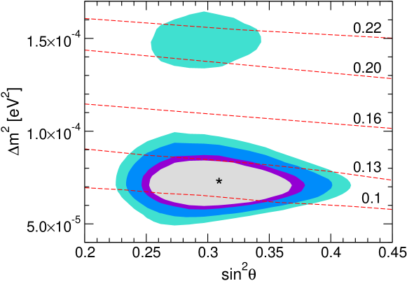
Figure 3: Similar as Fig. 1. The curves are iso-flux contours with the anti-neutrino yield fixed at the current KamLAND limit on $\phi_{\bar{\nu}_{e}}$ and corresponding to different values of $\varepsilon S\mu_{11}$. For values above 0.15 or so the high LMA region is ruled out.

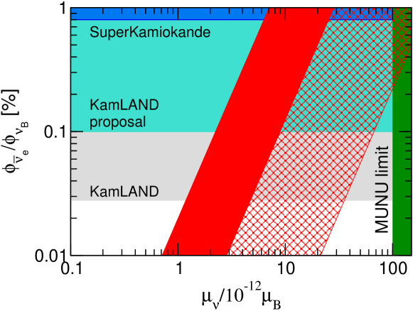
Figure 4: Bounds on $\mu_{\nu}$ for the turbulent magnetic field model described in the text. The horizontal lines indicate the bounds on solar electron anti-neutrino fluxes from Super-K and KamLAND. The diagonal dark band shows the limit on the intrinsic neutrino magnetic moment, its width corresponds to our (Kolmogorov) turbulent magnetic field model uncertainties. The crossing of this band with the lowest KamLAND line gives the limit $\mu_{\nu}=5\times 10^{-12}$ $\mu_{B}$. For comparison the vertical line indicates the present MUNU reactor limit. A more conservative and pessimistic limit discussed in Sec. V would give the limit indicated by the hatched band.

An important issue arises here, namely the robustness of the bounds we have obtained with respect to different possible choices of the scaling law for the turbulent kinetic spectrum. In order to answer this question we have considered the Iroshnikov-Kraichnan model 1983flma….3…..Z , characterized by the power law $p=3/2$ instead of $p=5/3$ that corresponds to the Kolmogorov spectrum. We have found that, in this case, the anti-neutrino yield is higher by $\sim 30$%, implying a correspondingly stronger bound on the neutrino magnetic moment. In general, values of $p$ lower than $5/3$ lead to the same tendency: the smaller $p$, the stronger limit on the neutrino magnetic moment.

Another question which may be addressed is whether different power-laws could be distinguished in future experiments, should solar electron anti-neutrinos ever be measured. Although the anti-neutrino yield is larger for the Iroshnikov-Kraichnan spectrum than for the Kolmogorov one, the expected anti-neutrino spectrum is not significantly different. In Fig. 5 the predicted anti-neutrino spectra (normalized to unity) are plotted both for the Iroshnikov-Kraichnan and Kolmogorov spectra. For comparison we have also shown the expected electron anti-neutrino spectrum for the random magnetic field case with $L_{0}=100$km and for the Kutvitsky-Soloviev magnetic field scenario Kutvitskii . One can see that there is no essential difference between them. Therefore, if a positive anti-neutrino signal is ever detected, the spectrum shape would not convey definitive information about the turbulent energy spectrum. In contrast, different $L_{0}$ values in random field scenario lead to significantly different energy spectrum predictions. This may help in some cases to distinguish these models, but the detailed analysis of this phenomenon is out of the scope of the paper.

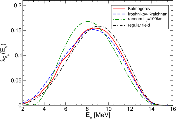
Figure 5: Predicted normalized electron anti-neutrino spectrum for the MHD turbulent model with Kolmogorov (solid) or Iroshnikov-Kraichnan (dashed) scaling exponents and the simplest random magnetic field model. For comparison we also indicate the expectation for the a regular magnetic field model.

Note that in the framework of our turbulent picture there is no time dependence in the magnetic field correlators, so that the resulting solar neutrino fluxes will have no time variation. This is a reasonable aproximation since the neutrino data we use are taken over periods larger than characteristic turbulent time fluctuations of solar magnetic fields. Possible neutrino flux variations in the Super-Kamiokande data have been considered Sturrock:2003kv ; Yoo:2003rc . We note however that in the framework of the spin flavour precession of Majorana neutrinos, irrespective of the magnetic field model adopted, the expected variations in the electron and muon neutrino fluxes should not exceed the current electron anti-neutrino flux bound $2.8\cdot 10^{-4}\phi_{B}$. Therefore time variations are expected to be too small, given the current statistical errors in the solar neutrino data.

V A critique of the robustness of the bound obtained

We now discuss in more detail the possible weaknesses of the method we have employed to constrain the neutrino magnetic moment in the case of turbulent magnetic fields. The bound is given from Eq. (34) and depends on $L_{\rm{max}}$. We have taken $L_{\rm{max}}\sim 1,000$ km, arguing that this is the size of the granules on the surface of the Sun. One might argue, however, that the scale $L_{max}$ may be associated with the size of the convection cells which is about a few $\times 10^{4}$ km. In such a worse-case scenario the neutrino conversion would be smaller, thus weakening the limit. However at most this would weaken our bound by a factor $(\rm{few}\times 10)^{1/3}\sim 3$ due to the mild power dependence 1/3. Moreover, the size of the largest turbulent eddies, $L_{\rm{max}}$, is still an open question, see for example Ref. 1983flma….3…..Z .

The bound on the neutrino magnetic moment also depends on the shape factor $0.5<S<1$. Such shape factor $S$ accounts for the fact that the random magnetic field may not be located in the whole convective zone (see discussion after Eq. (25)). The bound on the neutrino magnetic moment assuming that the shape factor is S=0.5 is a conservative bound and corresponds to the assumption that only 1/4 part of the convective zone is effectively filled by the random magnetic field ($S^{2}=0.25$).

The strength of the random (as well as the regular) magnetic field in the solar convective zone is unknown. There are different theoretical estimates of its value based on available experimental data. In order to derive our conservative limit on the neutrino magnetic moment we have used the value 50kG. A smaller value, say 20kG, for the strength of the large–scale regular magnetic field in the convective zone would result in a limit only 2.5 times weaker than the value we obtained. However we stress that the small–scale random magnetic field is expected to be comparable or even larger than the regular one. The value of 50 kG for the random magnetic field does not contradict the helioseismic data, in particular the analyses of SOHO MDI or GONG data. For example, the observed asphericity of the inferred sound speed may be explained by a magnetic field at the bottom of the convective zone of strength 200-300kG Antia:2002ti . We mention also that recent results on the modelling of the sunspot generation suggest that the strength of the toroidal field at the base of the solar convective zone must be on the order of 100 kG or so newref2 in which case the bound would get stronger.

All in all, taking all of the uncertainties mentioned above into acount we find that, in the worst case, they will be able to weaken our bound at most by one order of magnitude (see Fig. 4). Still the resulting bound is better than the current direct experimental bound. This situation would, in our opinion, be extremely unlikely as it would require a conspiracy.

VI Conclusions

We have considered neutrino spin-flavor precession in stationary solar magnetic fields, treated perturbatively with respect to LMA-MSW neutrino oscillations. We have discussed the impact of the recent KamLAND constraint on the solar anti-neutrino flux on the solutions of the solar neutrino problem in the presence of Majorana neutrino transition magnetic moments. This leads to strong limits on neutrino spin-flavor precession, involving $\mu_{\nu}B$. We analysed these constraints for a number of models of solar magnetic fields, both regular as well as random. We found that for a turbulent solar random magnetic field model, one can find a rather stringent constraint on the intrinsic neutrino magnetic moment down to the level of $\mu_{\nu}\lesssim{\rm few}\times 10^{-12}\mu_{B}$, similar to bounds obtained from star cooling. Such magnetic moments would have no effect in the detection process, given current experimental sensitivities. We also discussed how, in the worst possible case, these limits might deteriorate at most by one order of magnitude. We note also that for the complementary case where there is no spin flavor precession in the Sun and the only effect of the neutrino magnetic moment happens in the detection process Grimus:2002vb the current sensitivity is weaker than found here Liu:2004ny . Therefore we conclude that turbulent solar magnetic fields provide an enhanced sensitivity to very small neutrino transition magnetic moments. We have also shown how our result is rather insensitive to the details of the assumed model of turbulent random magnetic field. We verified this explicitly for Kolmogorov’s and Iroshnikov-Kraichnan spectra. Should solar anti-neutrinos ever be detected, it is unlikely that this would be of help in testing the intrinsic scaling law $B(L)\propto L^{1/3}$ characterizing turbulence.

VII Acknowledgements

We thank V. B. Semikoz and D. D. Sokoloff for useful discussions. This work was supported by Spanish grant BFM2002-00345, by European RTN network HPRN-CT-2000-00148, by European Science Foundation network grant N. 86, and MECD grant SB2000-0464 (TIR). TIR and AIR were partially supported by the Presidium RAS and CSIC-RAS grants and RFBR grant 04-02-16386. OGM was supported by CONACyT-Mexico and SNI.

Appendix A 3-$\nu$ description of $\bar{\nu}_{e}$ production in solar random magnetic fields

To justify the validity of the 2-$\nu$ scenario one can generalize it to the 3-$\nu$ case. The probability of the solar electron anti-neutrino appearence at the surface of the Earth (averaged over the Sun-Earth distance) takes the form

$$P_{e\bar{e}} \approx |\mu_{12}|^{2}I_{12}\left\{c_{13}^{2}c_{12}^{2}P_{2L}(0.7)+c_{13}^{2}s_{12}^{2}P_{1L}(0.7)\right\}$$

$$+ |\mu_{23}|^{2}I_{23}\left\{c_{13}^{2}s_{12}^{2}P_{3L}(0.7)+s_{13}^{2}P_{2L}(0.7)\right\}$$

$$+ |\mu_{13}|^{2}I_{13}\left\{c_{13}^{2}c_{12}^{2}P_{3L}(0.7)+s_{13}^{2}P_{1L}(0.7)\right\}\,.$$

Here $\mu_{jk}$ are the transition magnetic moments; $s_{jk}$ and $c_{jk}$ are corresponding $\sin$ and $\cos$ of the 3-$\nu$ mixing angles ($\theta_{12}$ – solar, $\theta_{23}$ – atmospheric, $\theta_{13}$ – reactor mixing angles); $P_{jL}(r=0.7R_{\odot})$ are the solar neutrino probabilities at the bottom of the convective zone. The integrals $I_{jk}$ are the generalizations of Eq.(16)

$$I_{jk}=\frac{1}{2}\int^{L}_{0}dt_{1}\int^{L}_{0}dt_{2}(b_{+}(t_{1})b_{-}(t_{2})e^{-2i\delta_{jk}(t_{1}-t_{2})}+c.c.)\,,$$ (38)

where $\delta_{jk}=\Delta m_{jk}^{2}/4E$, $\Delta m_{jk}^{2}=m_{k}^{2}-m_{j}^{2}$. To derive the above equation we have used the perturbative approach, as in Sec.II, leaving only terms quadratic in magnetic moments in the final probabilities.

We can notice first that, at a very good approximation, one has $P_{3L}(0.7)=s_{13}^{2}\ll 1$ (see Grimus:2002vb and references therein). The $\nu_{3L}$ yield in the solar core propagates as in vacuum because matter effects are strongly suppressed, as $\delta_{23}\approx\delta_{13}\gg V_{MSW}$.

Therefore the second and third terms in Eq. (A) are proportional to $\sin^{2}\theta_{13}$. In order to estimate $I_{jk}$ we consider the simple random magnetic field model discussed in Sec.III.1

$$I_{jk}=\frac{b^{2}S^{2}}{\delta_{jk}^{2}}\frac{L}{L_{0}}\sin^{2}(\delta_{jk}L_{0})$$ (39)

and the turbulent magnetic field model discussed in Sec. III.2

$$I_{jk}=0.3\frac{b^{2}S^{2}LL_{max}}{(\delta_{jk}L_{max})^{5/3}}$$ (40)

Taking into account that solar and atmospheric mass splittings have significantly different scales, $\Delta m_{12}^{2}\ll\Delta m_{23}^{2}\approx\Delta m_{13}^{2}$, we obtain in both cases (random and turbulent) that $I_{23}\approx I_{13}\ll I_{12}$, which means that neutrino spin-flavor conversion in the channels $1-3$ and $2-3$ is strongly suppressed with respect to the $1-2$ channel.

We may conclude that possible constraints on $|\mu_{23}|^{2}$ and $|\mu_{13}|^{2}$ are very poor. They are strongly suppressed by two facts:

• $s_{13}^{2}<0.054$ ($3\sigma$ C.L.) Maltoni:2003da ,

• $0.018<\Delta m_{12}^{2}/\Delta m_{13}^{2}\approx\Delta m_{12}^{2}/\Delta m_{23}^{2}<0.053$ ($3\sigma$ C.L.) Maltoni:2003da .

Therefore the contribution of other channels involving $\mu_{23}$ and $\mu_{13}$ to electron anti-neutrino production is strongly suppressed both directly by the small value of the angle $\theta_{13}$ and by the small ratio of solar to atmospheric squared mass differences $\Delta_{sol}^{2}/\Delta_{atm}^{2}$. As a result we adopt the 2-$\nu$ picture, characterized by a single component of the transition magnetic moment matrix ($\mu_{12}$) as a very good approximate description of anti-neutrino production.

References

- (1) KamLAND Collaboration, K. Eguchi et al., Phys. Rev. Lett. 92, 071301 (2004), [hep-ex/0310047].
- (2) Super-Kamiokande Collaboration, Y. Gando et al., Phys. Rev. Lett. 90, 171302 (2003), [hep-ex/0212067].
- (3) B. Aharmim et al. [SNO Collaboration], arXiv:hep-ex/0407029.
- (4) J. Schechter and J. W. F. Valle, Phys. Rev. D24, 1883 (1981), Err. Phys. Rev. D25, 283 (1982).
- (5) E. K. Akhmedov, Phys. Lett. B213, 64 (1988).
- (6) C.-S. Lim and W. J. Marciano, Phys. Rev. D37, 1368 (1988).
- (7) KamLAND Collaboration, K. Eguchi et al., Phys. Rev. Lett. 90, 021802 (2003), [hep-ex/0212021].
- (8) J. Barranco et al., Phys. Rev. D66, 093009 (2002), [hep-ph/0207326, version 3 which contains the KamLAND-update].
- (9) S. N. Ahmed et al. [SNO Collaboration], Phys. Rev. Lett. 92, 181301 (2004) [arXiv:nucl-ex/0309004].
- (10) M. Maltoni, T. Schwetz, M. A. Tortola and J. W. F. Valle, Phys. Rev. D68, 113010 (2003), [hep-ph/0309130]. For a recent review see M. Maltoni et al., New J. Phys. 6 122 (2004) http://stacks.iop.org/1367-2630/6/122, arXiv:hep-ph/0405172.
- (11) O. G. Miranda, T. I. Rashba, A. I. Rez and J. W. F. Valle, Phys. Rev. Lett. 93, 051304 (2004) [hep-ph/0311014]
- (12) A. A. Bykov, V. Y. Popov, A. I. Rez, V. B. Semikoz and D. D. Sokoloff, Phys. Rev. D59, 063001 (1999), [hep-ph/9808342].
- (13) V. A. Kutvitskii and L. S. Solov’ev, J. Exp. Theor. Phys. 78, 456 (1994).
- (14) M. M. Guzzo and H. Nunokawa, Astropart. Phys. 12, 87 (1999), [hep-ph/9810408].
- (15) E. K. Akhmedov and J. Pulido, Phys. Lett. B553, 7 (2003), [hep-ph/0209192]. B. C. Chauhan, J. Pulido and E. Torrente-Lujan, Phys. Rev. D 68 (2003) 033015 [arXiv:hep-ph/0304297].
- (16) A. Friedland and A. Gruzinov, Astropart. Phys. 19, 575 (2003), [hep-ph/0202095].
- (17) I. B. Zeldovich, A. A. Ruzmaikin and D. D. Sokolov, Magnetic fields in astrophysics (New York, Gordon and Breach Science Publishers), 1983.
- (18) G. G. Raffelt, Phys. Rev. Lett. 64, 2856 (1990).
- (19) E. Torrente-Lujan, JHEP 04, 054 (2003), [hep-ph/0302082].
- (20) F. N. Loreti and A. B. Balantekin, Phys. Rev. D50, 4762 (1994), [nucl-th/9406003].
- (21) H. Nunokawa, A. Rossi, V. B. Semikoz and J. W. F. Valle, Nucl. Phys. B472, 495 (1996), [hep-ph/9602307].
- (22) A. B. Balantekin and H. Yuksel, Phys. Rev. D68, 013006 (2003), [hep-ph/0303169].
- (23) M. M. Guzzo, P. C. de Holanda and N. Reggiani, Phys. Lett. B569, 45 (2003), [hep-ph/0303203].
- (24) A. Nicolaidis, Phys. Lett. B262, 303 (1991).
- (25) V. B. Semikoz and E. Torrente-Lujan, Nucl. Phys. B556, 353 (1999), [hep-ph/9809376].
- (26) C. P. Burgess and D. Michaud, Annals Phys. 256, 1 (1997), [hep-ph/9606295].
- (27) C. Burgess et al., Astrophys. J. 588, L65 (2003), [hep-ph/0209094].
- (28) C. P. Burgess et al., JCAP 0401, 007 (2004), [hep-ph/0310366].
- (29) P. Bamert, C. P. Burgess and D. Michaud, Nucl. Phys. B513, 319 (1998), [hep-ph/9707542].
- (30) K. Subramanian, Phys. Rev. Lett. 83, 2957 (1999), [astro-ph/9908280].
- (31) O. G. Miranda et al., Proc. of International Workshop on Astroparticle and High Energy Physics, October 14 - 18, 2003, Valencia, Spain, published at JHEP, PRHEP-AHEP2003/072, accessible from http://ific.uv.es/ahep/.
- (32) O. G. Miranda et al., Nucl. Phys. B595, 360 (2001), [hep-ph/0005259].
- (33) A. S. Monin and A. M. Yaglom, Statistical Fluid Mechanics, MIT Press, (Cambridge, 1975).
- (34) A. N. Kolmogorov, Dokl. Akad. Nauk. SSSR. 31, 538 (1941).
- (35) A. N. Kolmogorov, Proc. Roy. Soc. Lond. A434, 15 (1991).
- (36) P. Goldreich and S. Sridhar, Astrophys. J. 438, 763 (1995).
- (37) J. Cho and E. T. Vishniac, Astrophys. J. 539, 273 (2000).
- (38) M. Stix, The Sun. an Introduction (Springer-Verlag Berlin Heidelberg New York.
- (39) J. N. Bahcall and M. H. Pinsonneault, Phys. Rev. Lett. 92, 121301 (2004) [arXiv:astro-ph/0402114].
- (40) KamLAND Collaboration, J. Busenitz et al., Stanford-HEP-98-03, [http://kamland.lbl.gov/TalksPaper/].
- (41) MUNU Collaboration, Z. Daraktchieva et al., Phys. Lett. B564, 190 (2003), [hep-ex/0304011].
- (42) P. A. Sturrock, Astrophys. J. 605, 568 (2004), [hep-ph/0309239].
- (43) Super-Kamiokande Collaboration, J. Yoo et al., Phys. Rev. D68, 092002 (2003), [hep-ex/0307070].
- (44) W. Grimus et al., Nucl. Phys. B648, 376 (2003), [hep-ph/0208132].
- (45) H. M. Antia, S. M. Chitre and M. J. Thompson, Zone,” Astron. Astrophys. 399, 329 (2003) [arXiv:astro-ph/0212095].
- (46) D. Nandy and A. Rai Choudhuri, Science 296 (2002) 1671.
- (47) D. W. Liu et al. [Super-Kamiokande Collaboration], arXiv:hep-ex/0402015.